
Front. Comput. Sci.
DOI 10.1007/s11704-012-2002-5
Linking temporal records
Pei LI
1
, Xin Luna DONG
2
, Andrea MAURINO
1
,DiveshSRIVASTAVA
2
1 University of Milan-Bicocca, Milan 20126, Italy
2 AT&T Labs-Research, Florham Park, NJ 07932, USA
c
Higher Education Press and Springer-Verlag Berlin Heidelberg 2012
Abstract Many data sets contain temporal records which
span a long period of time; each record is associated with a
time stamp and describes some aspects of a real-world en-
tity at a particular time (e.g., author information in DBLP).
In such cases, we often wish to identify records that describe
the same entity over time and so be able to perform interest-
ing longitudinal data analysis. However, existing record link-
age techniques ignore temporal information and fall short for
temporal data.
This article studies linking temporal records. First, we ap-
ply time decay to capture the effect of elapsed time on en-
tity value evolution. Second, instead of comparing each pair
of records locally, we propose clustering methods that con-
sider time order of the records and make global decisions.
Experimental results show that our algorithms significantly
outperform traditional linkage methods on various temporal
data sets.
Keywords temporal data, record linkage, data integration
1 Introduction
Record linkage takes a set of records as input and discovers
which records r efer to the same real-world en tity. It plays
an important role in data integration, data aggregation, and
personal information management, and has been extensively
studied in recent years (see [1,2] for recent surveys). Exist-
ing techniques typically proceed in two steps: the first step
compares the similarity of each pair of records, deciding if
Recei ved January 01, 2012; accepted February 02, 2012
E-mail: [email protected]
they match or not; the second step clusters the records ac-
cordingly, with the goal that records in the same cluster refer
to the same real-world en tity and records in different clusters
refer to different ones.
In practice, a data set may contain temporal records over
a long period of time; each record is associated with a time
stamp and describes so me aspects of a real-world entity at
that particular time. In such cases, we often wish to identify
records that describe the same real-world entity over time
and so be able to tr ace the history of that entity. For exam-
ple, DBLP
1)
lists research papers over many decades; we
wish to identify individual authors such that we can list all
publications by each author. Other examples include med-
ical data that keep patient information over tens of years,
customer-relationship data that contains customer informa-
tion over y ears, and so on; identifying records that refer to
the same entity enables interesting longitudinal data analysis
over such data [3].
Although linking temporal records is important, to the best
of our knowledge, traditional techniques ignore the tempo-
ral information in linkage. Thus, they can fall short for such
data sets for two reasons. First, the same real- world entity
can evolve over time (e.g., a person can change their phone
number and address) and so records that describe the same
real-world entity at different times can contain different val-
ues; blindly requiring value consistency of the linked records
can thus cause false negatives. Second, it is more likely to
find highly similar entities over a long time period than at
the same time (e.g., having two persons with highly similar
names in the same university over the past 30 years is more
likely than at the same time) and so records that describe dif-
ferent entities at different times can share common values;
1)
http://www.dblp.org/

2 Front. Comput. Sci.
blindly matching records that have similar attribute values
can thus cause false positives. We illustrate the challeng es
with the following example.
Example 1 Consider records that describe paper authors in
Table 1; each record is derived from a publication record at
DBLP (we skip some co-authors for brevity). These records
describe 3 real-world people: r
1
describes E
1
: Xin Dong,who
was at R. Polytechnic in 1991; r
2
− r
6
describe E
2
: Xin Luna
Dong, who moved from Univ of Washington to AT&T Labs;
r
7
− r
12
describe E
3
: Dong Xin, who moved from Univ of
Illinois to Microsoft Research.
If we require high similarity on both name and a liation,
we may split entities E
2
and E
3
, as records for each of them
can have different values for a liation. If we require only
high similarity of name,wemaymergeE
1
with E
2
as they
share the same name, and may even merge all three entities.
Table 1 Records from DBLP
ID name a liation co-authors year
r
1
Xin Dong R. Polytechnic Institute Wozny 1991
r
2
Xin Dong Univ of Washington Hale vy, Tatarinov 2004
r
3
Xin Dong Univ of Washington Halevy 2005
r
4
Xin Luna Dong Univ of Washington Halevy, Yu 2007
r
5
Xin Luna Dong AT&T Labs-Research Das Sarma, Halevy 2009
r
6
Xin Luna Dong AT&T Labs-Research Naumann 2010
r
7
Dong Xin Univ of Illinois Han, Wah 2004
r
8
Dong Xin Univ of Illinois Wah 2007
r
9
Dong Xin Microsoft Research Wu, Han 2008
r
10
Dong Xin Univ of Illinois Ling, He 2009
r
11
Dong Xin Microsoft Research Chaudhuri, Ganti 2009
r
12
Dong Xin Microsoft Research Ganti 2010
Despite the challenges, temporal information presents ad-
ditional evidence for linkage. First, record values typically
transition smoothly. In the motivating example, person E
3
moved to a new affiliation in 2008, but still had similar co-
authors from previous years. Second, record values seldom
change erratically. In our example, r
2
, r
7
, r
3
, r
8
, r
10
(time or-
dered) are very unlikely to refer to the same person, as a per-
son rarely moves between two affiliations back and forth over
many years (however, this can happen around transition time;
for example, entity E
3
has a paper with the old affiliation in-
formation after he moved to a new affiliation, as shown by
record r
10
). Third, in case we have a fairly complete da ta set,
such as DBLP, records that refer to the same real-world en-
tity often (but not necessarily) observe continuity;forexam-
ple, one is less confident that r
1
and r
2
− r
6
refer to the same
person given the big time gap between them. Exploring such
evidence would require a global view o f the records with the
time factor in mind.
This article studies linking temporal records and makes
three contributions. First, we apply time decay, which aims
to capture the effect of time elapse on en tity value evolu-
tion (Section 3). In particular, we define disagreement decay,
with which value difference over a long time is not necessar-
ily taken as a strong indicator of referring to different real-
world entities; we define agreement decay, with which the
same value with a long time gap is not necessarily taken as a
strong indicator of referring to the same entity. We describe
how we learn decay from labeled data and how we apply it
when computing similarity between records.
Second, instead of comparing each pair of records locally
and then clustering, we describe three temporal clustering
methods that consider records in time order and accumulate
evidence over time to enable global decision making (Sec-
tion 4). Among them, early binding makes eager decisions
and merges a record with an already created cluster once it
computes a high similarity; late binding instead keeps all ev-
idence and makes decisions at the end; and adjusted binding
in addition compares a record with clusters that are cr eated
for records with later time stamp s.
Finally, we apply our methods on a European patent data
set and two subsets of the DBLP data set. Our experimen-
tal results show that applying decay in traditional methods
can improve the quality of linkage results, and applying our
clustering methods can obtain results with high precision and
recall (Section 5).
This article focuses on improving quality (precision an d
recall) of linking temporal records. We can further improve
efficiency of linkage by applying previous techniques such as
canopy [4] to create small blocks of records that are candi-
dates for temporal linkage.
This article is an extended version of a previous confer-
ence paper [5]. We describe in detail more alternative so-
lutions, including two additional decay learning algorithms,
and the probabilistic adjusting algor ithm for adjusted binding
and present experimental results comparing them. We also
give detailed proofs and describe more experimental results
showing the effectiveness and robustness of our results. Note
that in our work we assume the existence of temporal infor-
mation in the temporal records. Recent work [6] discussed
how to derive temporal ordering of records when time stamps
are absent; combining our techniques with techniques in [6]
would be interesting future work.
2Overview
This section formally defines the temporal record linkage

Pei LI et al. Linking temporal records 3
problem (Section 2.1) and provides an overview of our ap-
proach (Section 2.2).
2.1 Problem definition
Consider a domain D of object entities (not known a-prio ri)
where each entity is de scribed by a set of attributes A =
{A
1
,...,A
n
} and values of an attribute can change over time
(e.g., affiliation, business addresses). We distinguish single-
valued and multi-valued attributes, where the difference is
whether an attribute of an entity can have single or multiple
values at any time. Consider a set R of records, each is asso-
ciated with a time stam p and describing an entity in D at that
particular time. Given a record r ∈ R, we denote by r.t the
time stamp of r and by r.A the value of attr ibute A ∈ A from
r (we allow null as a value). Our goal is to decide which
records in R refer to the same entity in D.
Definition 1 (Temporal record linkage) Let R beasetof
records, each in the f orm of (x
1
,...,x
n
, t), where t is the time
stamp associated with the record, and x
i
, i ∈ [1, n], is the
value of attribute A
i
at time t for the referred entity.
The temporal record linkage problem clusters the records
in R such that records in the same cluster refer to the same
entity over time and records in different clusters refer to dif-
ferent entities.
Example 2 Consider the r ecords in Table 1, where each
record describes an author by name, a liation,andco-
authors (co-authors is a multi-valued attribute) and is as-
sociated with a time stamp (year). The ideal linkage solution
contains 3 clusters: {r
1
}, {r
2
,...,r
6
}, {r
7
,...,r
12
}.
2.2 Overview of our solution
Our record-linkage techniques leverage the temporal infor-
mationintwoways.
First, when computin g record sim ilarity, traditional link-
age techniques reward high value similarity and penalize low
value similarity. However, as time elapses, values of a partic-
ular entity may evolve; for example, a researcher may change
affiliation, email, and even name over time (see entities E
2
and E
3
in Example 1). Meanwhile, different entities are more
likely to share the same value(s) with a long time gap; for ex-
ample, it is more likely that we observe two persons with the
same name within 30 years than at the same time. We thus de-
fine decay (Section 3), with which we can reduce the penalty
for value disagreement and reduce the reward for value agree-
ment over a long period. Our experimental results show that
applying decay in similarity computation can improve over
traditional linkage techniques.
Second, when clustering records according to record simi-
larity, traditional techniques do not consider the time order of
the records. However, time order can o ften provide important
clues. In Example 1, records r
2
− r
4
and r
5
− r
6
may refer to
the same person even though the decayed similarity between
r
4
and r
6
is low, because the time period of r
2
− r
4
(year 2004-
2007) and that of r
5
− r
6
(year 2009-2010) do not overlap; on
the other hand, records r
2
− r
4
and r
7
, r
8
, r
10
are very likely to
refer to different persons even though the decayed similarity
between r
2
and r
10
is high, because the records interleave and
their occurrence periods highly overlap. We propose tempo-
ral clustering algorithms (Section 4) tha t consider time order
of records and can further improve linkage results.
3Timedecay
This section introduces time decay, an important concept that
aims at capturing the effect of time elapsing on value evo-
lution. Section 3.1 defines decay, Section 3.2 describes how
we learn decay, and Section 3 .3 describes how we apply de-
cay in similarity computation. Experimental results show that
by applying decay in traditional linkage techniques, we can
already improve the results.
3.1 Definition
As time goes by, the value of an entity may evolve; for exam-
ple, entity E
2
in Example 1 was at UW from 2004 to 2007,
and moved to AT&T Labs afterwards. Thus, different values
for a single-valued attribute over a long period of time should
not be considered as a strong indicator of referring to dif-
ferent entities. We define disagreement decay to capture this
intuition.
Definition 2 (Disagreement decay) Let Δt be a time dis-
tance and A ∈ A be a single-valued attribute. Disagreement
decay of A over time Δt, denoted by d
(A, Δt), is the proba-
bility that an entity changes its A-value within time Δt.
On the other hand, as time goes by, we are more likely to
observe two entities with the same attribute value; for exam-
ple, in Ex ample 1 entity E
1
occurred in 1991 and E
2
occurred
in 2004-2010, and they share the same name. Thus, the same
value over a long period of time should not be considered
as strong ind icator of referring to the same entity. We define
agreement decay accordingly.
Definition 3 ( Agreement decay) Let Δt be a time distance
4 Front. Comput. Sci.
and A ∈ A be an attribute. The agreement decay of A over
time Δt, denoted by d
=
(A, Δt), is the probability that two dif-
ferent entities share the same A-value within time Δt.
According to the definitions, decay satisfies two properties.
First, decay is in the range of [0,1]; however, d
(A, 0) and
d
=
(A, 0) are not necessarily 0, since even at the same time
their value-match does not necessarily correspond to record-
match and vice versa. Second, decay observes monotonicity;
that is, for any Δt < Δt
and any attribute A, d
(A, Δt)
d
(A, Δt
)andd
=
(A, Δt) d
=
(A, Δt
). Whereas our definition
of decay applies to all attributes, for attributes whose values
always remain stable (e.g., birth-date), the disagreement de-
cay is always 0, and for those whose values change rapidly
(e.g., bank-account-balance), the disagreement d ecay is al-
ways 1.
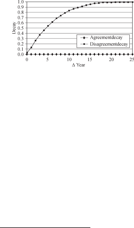
Example 3 Figure 1 shows the curves of disagreement de-
cay and agreement decay on attribute address learned from
a European patent data set (described in detail in Section 5).
Fig. 1 Decay curves for Address
We observe that (1) the disagreement decay increases from
0 to 1 as time elapses, showing that two records differing in
affiliation over a long time is not a strong indicator of refer-
ring to different entities; (2) the agreement decay is close to
0 everywhere, showing that in this data set, sharing the same
address is a strong indicator of referr ing to the same entity
even over a long time; (3) even when Δt = 0, neither the
disagreement nor the agreement d ecay is exactly 0, meaning
that even at the same time an address match does not defi-
nitely correspond to record match or mismatch.
3.2 Learning decay
Decay can be specified by domain experts or learned from a
labeled data set, for which we know if two records refer to the
same entity and if two strings represent the same value.
2)
For
simplification of computation, we make three assumptions.
1. Value uniqueness: at each time point an entity has a single
value for a single-valued attribute. 2. Closed-world: for each
entity described in the labeled data set, during the time pe-
riod when records that describe this entity are present, each
of its ever-existing values is reflected by some record and the
change is reflected at the transition point. 3. Correctness: val-
ues in each record reflect the truth in real world. The data
sets in practice often violate the assumptions. In our learning
we can resolve value-uniqueness conflicts with domain ex-
perts. Our experimental results show that the learned decay
does lead to good linkage results even when the latter two as-
sumptions are violated, as various kinds of violations in the
real data often cancel out each other in affecting the learned
curves. In addition, we relax the closed-world assumption
and propose probabilistic decay, but our experiments show
that it obtains very similar results to deterministic decay.
Consider attribute A and time period Δt. We n ext describe
three ways to calculate decay for A and Δt according to the
labels, namely, deterministic decay, single-count decay and
probabilistic decay.
3.2.1 Disagreement decay
By definition, disagreement decay for Δt is the probability
that an entity changes its A-value within time Δt. So we need
to find the valid period of each A-value o f an entity.
Consider an entity E and its records in increasing time or-
der, denoted by r
1
,...,r
n
, n 1. We call a time point t a
change point if at time t there exists a record r
i
, i ∈ [2, n],
whose A-value is different from r
i−1
. Additionally r
1
is al-
ways a change point. For each change point t (associated with
a new value), we can compute a life span:ift is not the final
change point of E, we call the life span of the current A-value
a full time span and denote it by [t, t
next
), where t
next
is the
next change point; otherwise, we call the life span a partial
time span and denote it by [t, t
end
+ δ), where t
end
is the final
time stamp for this value and δ denotes one time unit (in Ex-
ample 1, a unit of time is 1 year). A life span [t, t
) has length
t
− t, indicating that the corresponding value lasts for time
t
− t before any change in case of a full life span, and that
the value lasts at least for time t
− t in case of a partial life
span.
¯
L
f
denotes the bag of lengths of full life spans, and
¯
L
p
the bag of partial life spans.
Deterministic decay To learn d
(A, Δt), we consider all full
life spans and the partial life spans with length of at least Δt
(we cannot know for others if the value will change within
2)
In case there is no label for whether two strings represent the same value, we can easily extend our techniques by considering value similarity.

Pei LI et al. Linking temporal records 5
Δt). We compute the decay as
d
(A, Δt) =
|{l ∈
¯
L
f
|l Δt}|
|
¯
L
f
| + |{l ∈
¯
L
p
|l Δt}|
. (1)
We give details of the algorithm in Algorithm LearnDis-
agreeDecay (Algorithm 1). We can prove that the decay it
learns satisfies the monotonicity property.
Proposition 1 Let A be an attribute. For any Δt < Δt
,the
decay learned by Algorithm LearnDisagreeDecay satisfies
d
(A, Δt) d
(A, Δt
).
Algorithm 1 LearnDisagreeDecay(
¯
C, A)
Input:
¯
C Clusters of records in the sample data set, where records in the
same cluster refer to the same entity and records in different clusters
refer to different entities.
A Attribute for learning decay.
Output: Disagreement decay d
(Δt, A).
1:
¯
L
f
= φ;
¯
L
p
= φ;
2: for each C ∈
¯
C do
3: sort records in C in increasing time order to r
1
,...,r
|C|
;
4: // Find life spans
5: start = 1;
6: while start |C| do
7: end = star t + 1;
8: while r
start
.A = r
end
.A and end |C| do
9: end ++;
10: end while
11: if end > |C| then
12: insert r
|C|
.t − r
start
.t + δ into
¯
L
p
; // partial life span
13: else
14: insert r
end
.t − r
start
.t into
¯
L
f
; // full life span
15: end if
16: start = end;
17: end while
18: end for
19: // learn decay
20: for Δt = 1,...,max
l∈
¯
L
f
∪
¯
L
p
{l} do
21: d
(A, Δt) =
|{l∈
¯
L
f
|lΔt}|
|
¯
L
f
|+|{l∈
¯
L
p
|lΔt}|
22: end for
Proof In LearnDisagreeDecay,asΔt increases, |{l ∈
¯
L
f
|l
Δt}| is non-decreasing while |{l ∈
¯
L
p
|l Δt}| is non-
increasing; thus,
|{l∈
¯
L
f
|lΔt}|
|
¯
L
f
|+|{l∈
¯
L
p
|lΔt}|
is non-decreasing.
Example 4 Consider learning disagreement decay for al-
iation fro m the data in Example 1. For illustrative purposes,
we remove record r
10
as its affiliation information is incor-
rect. Take E
2
as an example. As shown in Fig. 2, it has two
change points: 2004 and 2009. So there are two life spans:
[2004, 2009) has length 5 and is full, and [2009, 2011) has
length 2 and is partial.
Fig. 2 Learning d
(a , Δt)
After considering other entities, we have
¯
L
f
= {4, 5} and
¯
L
p
= {1, 2, 3 }. Accordingly, d
(a , Δt ∈ [0, 1]) =
0
2+3
= 0,
d
(a , Δt = 2) =
0
2+2
= 0, d
(a , Δt = 3) =
0
2+1
= 0,
d
(a , Δt = 4) =
1
2
= 0.5, and d
(a , Δt 5) =
2
2
= 1.
Single-count decay We consider an entity at most on ce and
learn the disagreement decay d
(A, Δt) as the fraction of enti-
ties that have changed their A-value within time Δt. I n partic-
ular, if an entity E has full life spans, we choose the shortest
and insert its length l to
¯
L
f
, indicating that E has changed its
A-value in time l; otherwise, we consider E’s partial life span
and insert its length l to
¯
L
p
, indicating that E has not changed
its A-value in time l, but we do not know if it will change its
A-value after any longer time. We learn disagreement decay
using Eq. (1).
Proposition 2 Let A be an attribute. For any Δt < Δt
,the
decay learned using Single-count decay satisfies d
(A, Δt)
d
(A, Δt
).
Proof In single-count decay,asΔt increases, |{l ∈
¯
L
f
|l
Δt}| is non-decreasing while |{l ∈
¯
L
p
|l Δt}| is non-
increasing; thus,
|{l∈
¯
L
f
|lΔt}|
|
¯
L
f
|+|{l∈
¯
L
p
|lΔt}|
is non-decreasing.
Example 5 Consider learning disagreement decay for af-
liation from the following data: entity E
1
has two full life
spans, [2000, 2005), [2005, 2009), and one partial life span
[2009, 2011); entity E
2
has one partial life span [2003, 2010).
For E
1
, we consider its shor test f ull life span, which has
length 4; for E
2
, we consider its partial life span, which has
length 7. Therefore, we have
¯
L
f
= {4 },and
¯
L
p
= {7 }. Accord-
ingly, d
(a , Δt ∈ [0, 3]) =
0
1+1
= 0, d
(a , Δt ∈ [4, 7]) =
1
1+1
= 0.5, d
(a , Δt 8) =
1
1+0
= 1.
For comparison, on the same data set LearnDisagreeDe-
cay learns the following disagreement decay: d
(a , Δt ∈
[0, 3]) = 0, d
(a , Δt = 4) =
1
2+1
= 0.33, d
(a , Δt ∈
[5, 7]) =
2
2+1
= 0 .67, d
(a , Δt 8) =
2
2+0
= 1. So the
decay learned by LearnDisagreeDecay is smoother.

6 Front. Comput. Sci.
Probabilistic decay We remove the closed-world assump-
tion; that is, each value change is reflected by a record at
the change point. In particular, considering a full life span
[t, t
next
)weassumethelasttimeweseethesamevalueis
t
, t t
t
next
. We assume the value can change at any time
from t
to t
next
with equal probability
1
t
next
−t
+1
. Thus, for each
t
0
∈ [t
, t
next
], we insert length t
0
− t into
¯
L
f
and annotate it
with probability
1
t
next
−t
+1
.Ifwedenotebyp(l) the probability
for a particular length l in
¯
L
f
, we compute the disagreement
decay as
d
(A, Δt) =
l∈
¯
L
f
,lΔt
p(l)
l∈
¯
L
f
p(l) + |{l ∈
¯
L
p
|l Δt}|
. (2)
Proposition 3 Let A be an attribute. For any Δt < Δt
,the
decay learned using Probabilistic decay satisfies d
(A, Δt)
d
(A, Δt
).
Proof In probabilistic decay,asΔt increases,
l∈
¯
L
f
,lΔt
p(l)
is non-decreasing while |{l ∈
¯
L
p
|l Δt}| is non-increasing;
thus,
l∈
¯
L
f
,lΔt
p(l)
l∈
¯
L
f
p(l)+|{l∈
¯
L
p
|lΔt}|
is non-decreasing.
Example 6 Consider learning disagreement decay for af-
liation from the data set in Example 1. Again, we remove
record r
10
for illustrative purpose. Take E
2
as an example. Its
first affiliation has full life span [2004, 2009), and its last time
stamp is 2007. We consider the change can occur in any year
from 2007 to 2009, each with probability
1
2009−2007+1
=
1
3
.So
we insert length 3, 4, 5into
¯
L
f
, each with probability
1
3
. Simi-
larly, we insert length 3, 4 for entity E
3
, each with probability
0.5.
Eventually, we have
¯
L
f
= {3(
1
3
), 4(
1
3
), 5(0.33), 3(0.5),
4(0.5)},and
¯
L
p
= {1 , 2, 3 }. Accordingly, d
(a , Δt ∈ [0, 1]) =
0
2+3
= 0, d
(a , Δt = 2) =
0
2+2
= 0, d
(a , Δt = 3) =
0.5+0.33
2+1
= 0.28, d
(a , Δt = 4) =
0.33+0.33+0.5+0.5
2
= 0.84, and
d
(a , Δt 5) =
0.33+0.33+0.33+0.5+0.5
2
= 1.
Recall that for the same data set LearnDisagreeDecay
learns the following decay: d
(a , Δt ∈ [0, 3]) = 0,
d
(a , Δt = 4) = 0.5, and d
(a , Δt 5) = 1. Thus, the
curve learned by LearnDisagreeDecay is less smooth.
Experimental results (Section 5) show that these three
methods learn similar (but more or less smooth) decay curves,
and their results lead to similar linkage results.
3.2.2 Agreement decay
By definition, agreement decay for Δt is the proba bility that
two different entities share the same value within time period
Δt. Consider a value v of attribute A. Assume entity E
1
has
value v with life span [t
1
, t
2
)andE
2
has value v with life span
[t
3
, t
4
). Without losing generality, we assume t
1
t
3
. Then,
for any Δt max{0, t
3
− t
2
+ δ}, E
1
and E
2
share the same
value v within a period of Δt. We call max{0, t
3
− t
2
+ δ} the
span distance for v between E
1
and E
2
.
3)
Algorithm 2 LearnAgreeDecay(
¯
C, A)
Input:
¯
C Clusters of records in the sample data set, where records in the
same cluster refer to the same entity and records in different clusters
refer to different entities.
A An attribute for decay learning.
Eneure: Agreement decay d
=
(Δt, A).
1: //Find life spans
2: for each C ∈
¯
C do
3: sort records in C in increasing time order to r
1
,...,r
|C|
;
4: start = 1;
5: while start |C| do
6: end = star t + 1;
7: while r
start
.A = r
end
.A and end |C| do
8: end ++;
9: end while
10: if end > |C| then
11: r
start
.t
next
= r
|C|−1
.t + δ; // partial life span
12: else
13: r
start
.t
next
= r
end
.t; // full life span
14: end if
15: start = end;
16: end while
17: end for
18: //learn agreement decay
19:
¯
L = φ
20: for each C, C
∈
¯
C do
21: same = false;
22: for each r ∈ C s.t. r.t
next
null do
23: for each r
∈ C
s.t. r.t
next
null do
24: if r.A = r
.A then
25: same = true;
26: if r.t r
.t then
27: insert max{0, r
.t − r.t
next
+ 1} into
¯
L;
28: else
29: insert max{0, r.t − r
.t
next
+ 1} into
¯
L;
30: end if
31: end if
32: end for
33: end for
34: if !same then
35: insert ∞ into
¯
L;
36: end if
37: end for
38: for Δt = 1,...,max
l∈
¯
L
{l} do
39: d
=
(A, Δt) =
|{l∈
¯
L|lΔt}|
|
¯
L|
40: end for
3)
We can easily e xtend to the case where v has multiple life spans for the same entity.

Pei LI et al. Linking temporal records 7
For any pair of entities, we find the shared values and com-
pute the corresponding span distance for each of them. If two
entities never share any value, we use ∞ as th e sp an distance
between them. We denote by
¯
L the bag of span distances and
compute the agreement decay as
d
=
(A, Δt) =
|{l ∈
¯
L|l Δt}|
|
¯
L|
. (3)
Algorithm LearnAgreeDecay (Algorithm 2) describes the
details and we next show monotonicity of its results.
Proposition 4 Let A be an attribute. For any Δt < Δt
,
the decay learned by Algorithm LearnAgreeDecay satisfies
d
=
(A, Δt) d
=
(A, Δt
).
Proof In LearnAgreeDecay,asΔt increases, |{l ∈
¯
L|l
Δt}| is non-decreasing; thus,
|{l∈
¯
L|lΔt}|
|
¯
L|
is non-decreasing.
Example 7 Consider learning agreement decay for name
from data in Example 1. As shown in Fig. 3, entities E
1
and E
2
share value Xin Dong, for which the life span for
E
1
is [1991, 1992) and that for E
2
is [2004, 2009). Thus, the
span distance between E
1
and E
2
is 2004 − 1992 + 1 = 13.
No oth e r pair of entities shares the same value; thus,
¯
L =
{13, ∞, ∞}. Accordingly, d
=
(name, Δt ∈ [0, 12]) =
0
3
= 0,
and d
=
(name, Δt 13) =
1
3
= 0.33.
Fig. 3 Learning d
=
(name, Δt)
Similarly, we can apply single-count decay or probabilistic
decay to learn agreement decay. We o mit the details here for
brevity.
3.3 Applying decay
Here we describe how we apply d ecay in record-similarity
computation. We first focus on single-valued attributes and
then extend our method for multi-valued attributes.
3.3.1 Single-valued attributes
When computing similarity between two records with a big
time gap, we often wish to reduce the penalty if they have
different values and reduce the reward if they share the same
value. Thus, we assign weights to the attributes according
to the d ecay; the lower the weight, the less important an
attribute is in the record-sim ilarity computation, so there is
a lower penalty for value disagreement or lower reward for
value agreement. This weight is decided both by the time gap
and by the similarity between the values (to decide whether
to apply agreement or disagreement decay). We denote by
w
A
(s, Δt) the weight of attribute A with value similarity s and
time difference Δt. Given records r and r
, we compute their
similarity as
sim(r, r
) =
A∈A
w
A
(s(r.A, r
.A), |r.t − r
.t|) · s(r.A, r
.A)
A∈A
w
A
(s(r.A, r
.A), |r.t − r
.t|)
.
(4)
Next we describe how we set w
A
(s, Δt). With probability s,
the two values are the same and we shall use the complement
of the agreement decay; with probab ility 1− s, they are differ-
ent and we shall use the complement o f the disagreement de-
cay. Thus, we set w
A
(s, Δt) = 1−s·d
=
(A, Δt)−(1−s)·d
(A, Δt).
In practice, we use thresholds θ
h
and θ
l
to indicate high sim-
ilarity and low similarity respectively, and set w
A
(s, Δt) =
1 − d
=
(A, Δt)ifs >θ
h
and w
A
(s, Δt) = 1 − d
(A, Δt)ifs <θ
l
.
Our experiments show robustness of our techniques with re-
spect to different settings of the thresholds.
Example 8 Consider records r
2
and r
5
in Example 1 and
we focus o n single-valued attributes name and a liation.
Assume the name similarity between r
2
and r
5
is 0.9 and
the affiliation similarity is 0. Suppose d
=
(name, Δt = 5) =
0.05, d
(a , Δt = 5) = 0.9, and θ
h
= 0.8. Then, the weight for
name is 1−0.05 = 0.95 and that for a liation is 1−0 .9 = 0.1.
So the similarity is sim(r
1
, r
2
) =
0.95×0.9+0.1×0
0.95+0.1
= 0.81. Note
that if we do not apply decay and assign the same weight
to each attribute, the similarity would become
0.5×0.9+0.5×0
0.5+0.5
=
0.45.
Thus, b y applying decay, we are able to merge r
2
− r
6
,de-
spite the affiliation change of the entity. Note however that we
will also incorrectly merge all records together because each
record has a high decayed similarity to r
1
.
3.3.2 Multi-valued attributes
In this subsection we consider multi-valued attributes such as
co-authors. We start by describing record-similarity compu-
tation with such attributes, and then describe how we learn
and apply decay for such attributes.
Multi-valued attr ibutes differ from single-valued attributes
in that the same entity can have multiple values for such at-
tributes, even at the same time; therefore, (1) having different
values for such attributes does not indicate record mismatch;

8 Front. Comput. Sci.
and (2) sharing the same value for such attributes is additio nal
evidence for record match.
Consider a multi-valued attribute A. Consider records r and
r
; r.A and r
.A each is a set of values. Then, the similarity be-
tween r.A and r
.A, denoted by s(r.A, r
.A), is computed by a
variant of Jaccard distance between the two sets.
s(r.A, r
.A) =
v∈r.A,v
∈r
.A,s(v,v
)>θ
h
s(v, v
)
min{|r.A|, |r
.A|}
. (5)
If the relationship between the entities and th e A-values is
one-to-many, we add the attribute similarity (with a certain
weight) to the record similarity between r and r
. I n particu-
lar, let sim
(r, r
) be the similarity between r and r
when we
consider all attributes and w
A
be the weig ht for attribute A,
then,
sim
(r, r
)
= min{1, sim(r, r
) +
multi−valued A
w
A
· s(r.A, r
.A)}. (6)
On the o ther hand, if the relationsh ip between the en tities
and the A-values are many-to-many, we apply Eq. (6) only
when sim(r, r
) >θ
s
,whereθ
s
is a threshold for high similar-
ity on values of single-valued attributes.
Now consider decay on such multi-valued attributes. First,
we do no t learn d isagreement decay on multi-valued at-
tributes but we learn agreement d ecay in the same way as for
single-valued attributes. Second, we apply agreement decay
when we compute the similarity between values of a multi-
valued attribute, so if the time gap between two similar values
is large, we discount the similarity. In particular, we revise
Eq. (5) as follows:
s(r.A, r
.A)
=
v∈r.A,v
∈r
.A,s(v,v
)>θ
h
(1 − d
=
(A, |r.t − r
.t|))s(v, v
)
min{|r.A|, |r
.A|}
. (7)
Example 9 Consider records r
2
and r
5
and multi-valued at-
tribute co-authors (many-to-many relationship) in Example
1. Let θ
h
= 0.8andw
co
= 0.3. Record r
2
and r
5
share one
co-author with string similarity 1. Suppose d
=
(co, Δt = 5) =
0.05. Then, s(r
2
.co, r
5
.co) =
(1−0.05)∗1
min{2,2}
= 0.475. Recall from
Example 8 that sim(r
2
, r
5
) = 0.81 >θ
h
; therefore, the overall
similarity is sim
(r
2
, r
5
) = min{1, 0 .81 + 0.475 ∗ 0.3} = 0.95.
4 Temporal clustering
As shown in Example 8, even when we apply decay in simi-
larity computation, traditional clustering methods do not nec-
essarily lead to good results as they ignore the time order
of the records. This section proposes three clustering meth-
ods, all processing the records in increasing time order. Early
binding (Section 4.1) makes eager decisions and merges a
record with an already created cluster once it computes a high
similarity between them. Late binding (Section 4.2) com-
pares a record with each already created cluster and keeps
the probability, and makes clustering decision at the end. Ad-
justed binding (Section 4.3) is applied after early binding or
late binding, and improves over them by comparing a record
also with clusters created later and adjusting the clustering
results. Our experimental results show that adjusted binding
significantly outperforms traditional clustering methods on
temporal data.
4.1 Early binding
Algorithm: Early binding considers the records in time or-
der; for each record it eagerly creates its own cluster or
merges it with an already created cluster. In particular, con-
sider record r and already created clusters C
1
,...,C
n
.Early
proceeds in three steps.
1. Compute the similarity between r and each C
i
, i ∈ [1, n].
2. Choose the cluster C with the highest similarity.
Merge r with C if sim(r, C) >θ,whereθ is a threshold
indicating high similarity; create a new cluster C
n+1
for
r otherwise.
3. Update signature for the cluster with r accordingly.
Cluster signature When we merge record r with cluster C,
we need to update the signature of C accordingly (step 3). As
we consider r as the latest record of C,wetaker’s values as
the latest values of C. For the purpose of similarity compu-
tation, which we describe shortly, for each latest value v we
wish to keep 1) its various representations, denoted by
¯
R(v),
and 2) its earliest and latest time stamps in the current period
of occurrence, denoted by t
e
(v)andt
l
(v) respectively. The lat-
est occurrence of v is clearly r.t. We m aintain the earliest time
stamp and various representations recursively as follows. Let
v
be the previous value of C,andlets
max
be the highest sim-
ilarity between v and the values in
¯
R(v
). (1) If s
max
>θ
h
,we
consider the two values as the same and set t
e
(v) = t
e
(v
)and
¯
R(v) =
¯
R(v
)∪{v}.(2)Ifs
max
<θ
l
, we consider the two values
as different and set t
e
(v) = r.t and
¯
R(v) = {v}. (3) Otherwise,
we consider that with probability s
max
the two values are the
same, so we set t
e
(v) = sim(v, v
)t
e
(v
) + (1 − sim(v, v
))r.t and
¯
R(v) =
¯
R(v
) ∪{v}.
Similarity computation When we compare r with a clus-

Pei LI et al. Linking temporal records 9
ter C (step 1), for each attribute A, we compare r’s A-value
r.A with the A-value in C’s signature, denoted by C.A.We
make two changes in this process: first, we compare r.A with
each value in
¯
R(C.A) and take the maximum similarity; sec-
ond, when we compute the weight for A,weuset
e
(C.A)for
disagreement decay as C.A starts from time t
e
(C.A), and use
t
l
(C.A) for agreement decay as t
l
(C.A) is the last time we see
C.A.
We describe Algorithm Early in Alg orithm 3. Early runs
in time O(|R|
2
); the quadratic time is in the number of records
in each block after preprocessing.
Algorithm 3 Early(R)
Input: R records in increasing time order
Output:
¯
C clustering of records in R
1: for each record r ∈ Rdo
2: for each C ∈
¯
C do
3: compute record-cluster similarity sim(r, C);
4: end for
5: if max
C∈
¯
C
sim(r, C) θ then
6: C = Argma x
C∈
¯
C
sim(r, C);
7: insert r into C;
8: update signature of C;
9: else
10: insert cluster {r} into
¯
C;
11: end if
12: end for
13: return
¯
C;
Example 10 Consider applying early binding to records in
Table 1. Table 2 shows the signature of a liation for each
cluster after we process each record. The change in each step
is in bold.
Table 2 Example 10: cluster signature in early binding
C
1
C
2
C
3
r
1
R.Poly, 1991-1991 --
r
2
UW, 2004-2004 --
r
7
UW, 2004-2004 UI, 2004-2004 -
r
3
UW, 2004-2005 UI, 2004-2004 -
r
8
UW, 2004-2005 UI, 2004-2007 -
r
4
UW, 2004-2007 UI, 2004-2007 -
r
9
UW, 2004-2007 MSR, 2008-2008 -
r
10
UI, 2009-2009 MSR, 2008-2008 -
r
11
UI, 2009-2009 MSR, 2008-2009 -
r
5
UI, 2009-2009 MSR, 2008-2009 AT&T, 2009-2009
r
12
UI, 2009-2009 MSR, 2008-2010 AT&T, 2009-2009
r
6
UI, 2009-2009 MSR, 2008-2010 AT&T, 2009-2010
We start with creating C
1
for r
1
. Then we merge r
2
with C
1
because of the high record similarity (same name and high
disagreement decay on a liation with time difference 2004-
1991=13). The new signature of C
1
contains address UW
from 2004 to 2004. We then create a new cluster C
2
for r
7
,
as r
7
differs significantly from C
1
.Next,wemerger
3
and r
4
with C
1
and merge r
8
and r
9
with C
2
. The signature of C
1
then
contains address UW from 2004 to 2007, and the signature of
C
2
contains address MSR from 2008 to 2008.
Now consider r
10
. It has a low similarity to C
2
(r
10
and r
9
has a short time distance but different affiliations), but a high
similarity to C
1
(fairly similar name and high disagreement
decay on a liation with time difference 2009 − 2004 = 5).
We thus wrongly merge r
10
with C
1
. This eager decision fur-
ther prevents merging r
5
and r
6
with C
1
and we create C
3
for
them separately.
4.2 Late binding
Instead of making eager decisions and comparing a record
with a cluster based on such eager decisions, late b inding
keeps all evidence, considers them in record-cluster compar-
ison, and makes a global decision at the end.
Late binding is facilitated by a b ipartite graph (N
R
, N
C
, E),
where each node in N
R
represents a record, each node in N
C
represents a cluster, and each edge (n
r
, n
C
) ∈ E is marked
with th e probability that record r belongs to cluster C (see
Fig. 4 for an example). Late binding clusters the records in
two stages: first, evidence collection creates th e bi-partite
graph and computes the weight for each edge; then, deci-
sion making removes edges such that each record belongs to
a single cluster.
Fig. 4 Example 11: A part of the bi-partite graph
4.2.1 Evidence collection
Late binding behaves similarly to early binding at the evi-
dence collection stage, except that it keeps all possibilities
rather than making eager decisions. For each record r and al-
ready created clusters C
1
,...,C
n
, it proceeds in three steps.
1. Compute the similarity between r and each C
i
, i ∈ [1, n].
2. Create a new cluster C
n+1
and assign similarity as fol-
10 Front. Comput. Sci.
lows. (1) If for each i ∈ [1, n], sim(r, C
i
) θ,we
consider that r is unlikely to belong to any C
i
and set
sim(r, C
n+1
) = θ. (2) If there exists i ∈ [1, n ], such
that not only sim(r, C
i
) >θ,butalsosim
(r, C
i
) >θ,
where sim
(r, C
i
) is computed by ignoring decay, we
consider that r is very likely to belong to C
i
and set
sim(r, C
n+1
) = 0. (3) Otherwise, we set sim(r, C
n+1
) =
max
i∈[1,n]
sim(r, C
i
).
3. Normalize the similarities such that they sum up to 1
and u se the results as probabilities of r belonging to each
cluster.
Update the signature of each cluster accordingly.
In the final step, we normalize the similarities such that the
higher the similarity, the higher the result probability. Note
that in contrast to early binding, late binding is conservative
when the record similarity without decay is low (Step 2(3));
this may lead to splitting records that have different values
but refer to the same entity, and we sh ow later how adju sted
binding can benefit from the conservativeness.
Edge deletion In practice, we may set low similarities to
0 to improve performance; we next describe several edge-
deletion strategies. Our experimental results (Section 5) show
that they obtain similar results, while they all improve over
not deleting edges in both efficiency and accuracy of the re-
sults.
• Thresholding removes all edges whose associated simi-
larity scores are less or equal to a threshold θ.
• Top-K keeps the top-k edges whose associated similar-
ity scores are above threshold θ.
• Gap orders the edges in descending order of the as-
sociated similarity scores to e
1
, e
2
,...,e
n
, and selects
the edges in decreasing order until reaching an edge e
i
where(1)thescoresfore
i
and e
i+1
have a gap larger
than a g iven threshold θ
gap
, or (2) the score for e
i+1
is
less than threshold θ.
Cluster signature For each cluster, the signature consists
of all records that may belong to the cluster along with the
probabilities. For each value of every record , we maintain the
earliest time stamp, the latest time stamp, and similar values,
as we do in early binding.
Similarity computation When we compare r with a clus-
ter C, we need to consider the prob a bility that a record in
C’s signature belongs to C.Letr
1
,...,r
m
be the records of
C in increasing time order, and let P(r
i
), i ∈ [1, m], be the
probability that r
i
belongs to C. Then, with probability P(r
m
),
record r
m
is the latest record of C and we should compare r
with it; with probability (1− P(r
m
))P(r
m−1
), record r
m−1
is the
latest record of C and we should compare r with it; and so
on. Note that the cluster is valid only when r
1
,forwhichwe
create the cluster, belongs to the cluster, so we use P(r
1
) = 1
in the computation (the original P(r
1
) is used in the decision-
making stage). Formally, the similarity is computed as
sim(r, C) =
m
i=1
sim(r, r
i
)P(r
i
)Π
m
j=i+1
(1 − P(r
i
)). (8)
Example 11 Consider applying late binding to the records
in Table 1 and let θ = 0.8. Figure 4 shows a part of the bi-
partite graph. At the beginnin g, we create an edge b e tween
r
1
and C
1
with weight 1. We then compare r
2
with C
1
:the
similarity with decay (0.89 >θ) is high but that without de-
cay (0.5 <θ) is low. We thus create a new cluster C
2
and set
sim(r
2
, C
2
) = 0.89. After normalization, each edge from r
2
has a weight of 0.5.
Now consider r
7
.ForC
1
, with probability 0.5 we shall
compare r
7
with r
2
(suppose sim(r
7
, r
2
) = 0.4) and with prob-
ability 1 − 0.5 = 0.5 we shall compare r
7
with r
1
(suppose
sim(r
7
, r
1
) = 0.8). Thus, sim(r
7
, C
1
) = 0.8 × 0.5 + 0.4 × 0 .5 =
0.6 <θ.ForC
2
, we shall compare r
7
only with r
2
and the sim-
ilarity is 0.4 <θ. Because of the low similarities, we create
anewclusterC
3
and set sim(r
7
, C
3
) = 0.8. After normaliza-
tion, the probabilities from r
7
to C
1
, C
2
and C
3
are 0.33, 0.22
and 0.45 respectively.
4.2.2 Decision making
The second stage makes clustering decisions according to the
evidence we have collected. We consider only valid cluster-
ings, where each non-empty cluster contains the record for
which we create the cluster. Let
¯
C be a clustering and we de-
note by
¯
C(r) the cluster to which r belongs in
¯
C. We can
compute the probability of
¯
C as Π
r∈R
P(r ∈
¯
C(r)), where
P(r ∈
¯
C(r)) de notes the probability that r belongs to
¯
C(r).
We wish to choose the valid clustering with the highest prob-
ability. Enumerating all clusterings and computing the prob-
ability for each of them can take exponential time. We next
propose an algorithm that takes only polynomial time and is
guaranteed to find the optimal solution.
1. Select the edge (n
r
, n
C
) with the highest weight.
2. Remove other edges connected to n
r
.
3. If n
r
is the first selected edge to n
C
but C is created for
record r
r, select the edge (n
r
, n
C
)andremoveall
other edges connected to n
r
(so the result clustering is

Pei LI et al. Linking temporal records 11
valid).
4. Go to Step 1 until all edges are either selected or re-
moved.
We describe algorithm Lat e in Algorithm 4 and next state
the optimality of the decision-making stage.
Algorithm 4 Lat e (R)
Input: R records in increasing time order
Output:
¯
C clustering of records in R
1: Initialize a bi-partite graph (N
R
, N
C
, E)whereN
R
= N
C
= E = ∅;
2: //Evidence collection
3: for each record r ∈ Rdo
4: insert node n
r
into N
R
;
5: for each n
C
∈ N
C
do
6: compute decayed record-cluster similarity sim(r, C);
7: end for
8: if max
n
C
∈N
C
sim(r, C) θ then
9: insert node n
C
r
into N
C
;
10: insert edge (n
r
, n
C
r
) with weight θ into E;
11: else
12: newCluster = true;
13: for each n
C
∈ N
C
,wheresim(r, C) >θdo
14: compute no decayed similarity sim
(r,C);
15: if sim
(r,C) >θthen
16: newCluster = false; break;
17: end if
18: end for
19: if newCluster then
20: insert node n
C
r
into N
C
;
21: insert edge (n
r
, n
C
r
) with weight
max
n
C
∈N
C
,sim
(r,C)>θ
(sim(r, C)) into E;
22: end if
23: end if
24: delete edges with low weights;
25: normalize weights for all edges from n
r
;
26: end for
27: // Decision making
28: while |E| > |N
R
| do
29: select edge (n
r
, n
C
) with maximal edge weight;
30: remove edges (n
r
, n
C
)forallC
C;
31: if cluster C is created for record r
r then
32: select edge (n
r
, n
C
);
33: remove edges (n
r
, n
C
)forallC
C;
34: end if
35: end while
36: return
¯
C;
Proposition 5 Lat e algorithm runs in time O(|R|
2
)and
chooses the clustering with the highest probability from all
possible valid clusterings.
Proof Our evidence collection step guarantees that if C
r
is
created for record r, then the edge (N
r
, N
C
r
) has the highest
weight among edges from N
r
. Thus, the decision making step
chooses the edge with the highest weight for each record and
obtains the optimal solution.
Example 12 Continuing from Example 11. After evidence
collection, we created 5 clusters and the weight of each
record-cluster pair is shown in Table 3. Weights of selected
edges are in bold.
Table 3 Example 12: weights on the bipartite graph
r
1
r
2
r
7
r
3
r
8
r
4
r
9
r
10
r
11
r
5
r
12
r
6
C
1
1 0.50.330.370.270.380.160.130.180.240.120.22
C
2
0 0.5 0.22 0.40 0.25 0.40 0.16 0.12 0.17 0.27 0.10 0.24
C
3
00 0.45 0.23 0.48 0.22 0.24 0.26 0.20 0.17 0.23 0.18
C
4
0000000.44 0.19 0.29 0.16 0.33 0.18
C
5
00000000.30 0.16 0.16 0.22 0.18
We first select edge (n
r
1
, n
C
1
) with weight 1. We th en
choose (n
r
2
, n
C
2
) with weight 0.5 (there is a tie between C
1
and C
2
; even if we choose C
1
at the beginning, we will
change back to C
2
when we select edge (n
r
3
, n
C
2
)), and
(n
r
8
, n
C
3
) with weight 0.48. As C
3
is created for record r
7
,
we also select edge (n
r
7
, n
C
3
) and remove other edges from
r
7
. We choose edges for the rest o f the records similarly
and the final result contains five clusters: {r
1
}, {r
2
,...,r
6
},
{r
7
, r
8
}, {r
9
, r
11
, r
12
}, {r
10
}.
Note that despite the error made for r
10
, we are still able to
correctly merge r
5
and r
6
with C
2
because we make the de-
cision at the end. Note however that we did not merge r
9
, r
11
and r
12
with C
3
, because of the conservativeness of late bind-
ing.
4.3 Adjusted binding
Neither early binding nor late binding compares a record with
a cluster created later. However, evidence from later records
may fix early errors; in Example 1, after observing r
11
and
r
12
, we are more confident that r
7
− r
12
refer to the same
entity but record r
10
has out-of-date affiliation informatio n.
Adjusted binding allows comparison between a record and
clusters that are created later.
Adjusted binding can start with the results from either early
or late binding and iteratively adjust the clustering (determin-
istic adjusting), or start with the bi-partite graph created from
evidence collection of late binding, and iteratively adjust the
probabilities (probabilistic adjusting). We next describe the
two algorithms.
4.3.1 Deterministic algorithm
Deterministic adjusting proceeds in EM-style.

12 Front. Comput. Sci.
1. Initialization: Set the initial assignment as the result of
early or late binding.
2. Estimation (E-step): Compute the similarity of each
record-cluster pair and normalize the similarities as in
late binding.
3. Maximization (M-step): Choose the clustering with the
maximum probability, as in late binding.
4. Termination: Repeat E-step and M-step until the results
converge o r oscillate.
Similarity computation The E-step compares a record r
with a cluster C, whose signature may contain records that
occur later than r. Our similarity computation takes advan-
tage of this complete view of value evolution as follows.
First, we consider consistency of the records, including
consistency in evolution of the values, in occurrence fre-
quency, and so on. We next describe how we compute value
consistency and occurrence frequency.
Consider the value consistency between r and C =
{r
1
,...,r
m
} (if r ∈ C, we remove r from C), denoted by
cons(r, C) ∈ [0, 1]. Assume the records of C areintimeorder
and r
k
.t < r.t < r
k+1
.t.
4)
Inserting r into C can affect the con-
sistency of C in two ways: 1) r may be inconsistent with r
k
,so
the similarity between r and the sub-cluster C
1
= {r
1
,...,r
k
}
is low; 2) r
k+1
may be inconsistent with r, so the similarity
between r
k+1
and the sub-cluster C
2
= {r
1
,...,r
k
, r} is low.
We take the minimum as cons(r, C),
cons(r, C) = min(sim( r, C
1
), sim(r
k+1
, C
2
)). (9)
Occurrence consistency considers a cluster C.Theoccur-
rence frequency of C, denoted by freq(C), is computed by
freq(C) =
C
late
− C
early
|C|
. (10)
Let C
be the cluster after inserting record r into C.
The occurrence consistency between r and C, denoted by
cons
f
(r, C) is computed by
cons
f
(r, C) = 1 −
| freq(C) − freq(C
)|
max{ freq(C) , freq(C
)}
. (11)
Second, we consider continuity of r and C’s other records
in time, denoted by cont(r, C) ∈ [0, 1]. Consider the five cases
in Fig. 5 and assume the same consistency between r and C.
Record r is farther away in time from C’s records in cases 1
and 5 than in cases 2—4, so it is less likely to belong to C in
cases 1 and 5. Let C.early denote the earliest time stamp of
records in C and C.late denote the latest one. We compute the
continuity as follows.
cont(r, C) = e
−λy
; (12)
y =
|r.t − C.early| + α
C.late − C.early + α
. (13)
Fig. 5 Continuity between record r and cluster C
Here, λ>0 is a parameter that controls the level of con-
tinuity we require; α>0 is a small number such that when
the denominator (resp. numerator) is 0, the numerator (resp.,
denom inator) can still affect the result
5)
. Under this defini-
tion, the higher the time difference between r and the earliest
record in C compared with the length of C, the lower the con-
tinuity. In Fig. 5, cont (r, C) is close to 0 in cases 1, 5, close to
1 in cases 2, 3, and close to e
−λ
in case 4. Note that we favor
time points close to C.early more than those close to C.late;
thus, when we merge two clusters that are close in time, we
will gradually move the latest record of the early cluster into
the late cluster, as it has a higher continuity with the late clus-
ter.
Finally, the similarity of r and C considers both consis-
tency and continuity, and is computed by
sim(r, C) = cons(r, C) · cont(r, C). (14)
Recall that late binding is conservative for records whose
similarity without decay is low and may split them. Adjusted
binding re-examines them and merges them only when they
have both high consistency and high continuity, and thus
avoids aggressive merging of records with big time gap.
We describe the detailed algorithm, Adjust, in Algorithm
5. Our experiments show that Adjust does not necessarily
converge, but the quality measures of the results at the oscil-
lating rounds are very similar.
4)
We can extend our techniques to the case when r has the same time stamp as some record in C.
5)
In practice, we set α to one time unit, and set λ = − ln cons where cons is the minimum consistency we require for merging a record with a cluster. When
we merge two clusters C
1
and C
2
where C
1
.late = C
2
.early, with such λ the latest record r
1
of C
1
has continuity cons with C
1
and continuity 1 with C
2
,so
can be merged with C
2
if cons(r
1
, C
2
) > cons.

Pei LI et al. Linking temporal records 13
Example 13 Consider r
10
and C
4
= {r
9
, r
11
, r
12
} in the re-
sults of Example 12. For value consistency, inserting r
10
into C
4
results in {r
9
,...,r
12
}. Assume sim(r
10
, {r
9
}) =
sim(r
11
, {r
9
,
r
10
}) = 0.6. Then, cons(r
10
, C
4
) = 0.6. For continuity, if we
set λ = 2andα = 1, we obtain l(r
10
, C
4
) = e
−2·
1+1
2+1
= 0.26.
Thus, the similar ity is 0.26 × 0.6 = 0.16. On the other hand,
the similarity between r
10
and C
5
is 1 · e
−2·
1
1
= 0.14. We thus
merge r
10
with C
4
.
Similarly, we then merge r
8
with C
4
and in turn r
7
with
C
4
, leading to the correct result. Note that we do not merge
r
1
with C
2
, because of the long time gap and thus a low con-
tinuity.
4.3.2 Probabilistic adjusting
Probabilistic adjusted binding proceeds in three steps.
• The algorithm starts with the b i-partite graph created
from evidence collection in late binding.
• It iteratively adjusts the weight of each edge and keeps
all edges, until the weights converge or oscillate.
In each iteration, it (1) re-computes the similarity be-
tween each record and each cluster, (2) normalizes the
weights of edges from the same record node, and (3)
re-computes the signature of each cluster.
• It selects the possible world with the highest probability
as in late binding.
Algorithm 5 Adjust(R,
¯
C)
Input: R records in increasing time order.
¯
C pre-clustering of records in R.
Output:
¯
C new clustering of records in R.
1: repeat
2: //E-step
3: for each record r ∈ Rdo
4: for each cluster C ∈
¯
C do
5: compute sim(r, C) = cons(r, C) ∗ cont(r, C);
6: end for
7: end for
8: //M-step
9: Choose the possible world with the highest probability as in Ln.28–
25 of Lat e ;
10: until
¯
C is not changed
11: return
¯
C;
In the second step, when we compute the similarity
between a record and a cluster, we compute consistency
cons(r, C) and continuity cont(r, C) similarly as in determin-
istic adjusted binding, except that we also need to consider
the probability of a record belonging to a cluster. For value
consistency, we consider probability in the same way as in
late binding. For continuity, we compute the probabilistic
earliest and latest time stamps of a cluster as follows. Sup-
pose cluster C is connected to m records r
1
,...,r
m
where
r
1
.t r
2
.t ··· r
m
.t, each with probability p
i
, i ∈ [1, m].
We compute C
early
and C
late
as follows:
C
early
=
m
i=1
r
i
.t · (p
i
Π
i−1
k=1
(1 − p
k
)). (15)
C
late
=
m
i=1
r
i
.t · (p
i
Π
m
k=i+1
(1 − p
k
)). (16)
Our experim ents (Section 5) shows that probabilistic ad-
justing takes much longer than deterministic adjusting, but
does not have an obvious performance gain.
5 Experimental evaluation
This section describes the results of experiments on two real
data sets. We show that (1) our technique significantly im-
proves o n traditional methods on various data sets; (2) the two
key components of our strategy, namely, decay and temporal
clustering, are both important for obtaining good results; (3)
our technique is robust with respect to various data sets and
reasonable parameter settings; (4) our techniques are efficient
and scalable.
5.1 Experiment settings
Data and golden standard We experimented on two real-
world data sets: a benchmark of European patent data set
6)
and the DBLP data set. From the patent data we extracted In-
ventor r ecords with attributes name and address; the time
stamp of each record is the patent filing date. The benchmark
involves 359 inventors from French patents, where different
inventors rarely share similar names; we thus increased the
hardness by deriving a data set with only first name and last
name initial for each inventor. We call the original data set
the full set and the derived one the partial set.
From the DBLP data we considered two subsets: the XD
data set contains 72 records for authors named Xin Dong,
Luna Dong, Xin Luna Dong,orDong Xin,forwhichwe
manually identified 8 authors; the WW data set contains 738
records for authors named Wei Wang, for 302 of which DBLP
has manually identified 18 authors (the rest is left in a pot-
6)
http://www.esf-ape-inv.eu/

14 Front. Comput. Sci.
pourri). For each subset we extracted Author records with
attributes name, a liation, and co-author (we extracted af-
liation information from the papers) o n 2/1/2011; the time
stamp of each record is the paper publication year. Table 4
shows statistics of the data sets.
Table 4 Statistics of the experimental data sets
#Records #Entities Years
Patent (full or partial) 1871 359 1978—2003
DBLP-XD 72 8 1991—2010
DBLP-WW 738 18+potpourri 1992—-2011
Implementation We learned d ecay from both patent data
sets. The decay we learned for the address attribute is shown
in Fig. 1 (Section 3); for name, both agreement and disagree-
ment decay are close to 0 on both data sets. We observed sim-
ilar linkage results when we learned the decays from half of
the data and applied them to the other half. We also applied
the decay learned from the partial data set on linking DBLP
records.
We pre-partitioned the records by the initial of the last
name, and implemented the following methods on each par-
tition.
• Baseline methods include Partition,Center,and
Merge [7]. They all compute pairwise record similar-
ity but apply different clustering strategies. We give the
details as follows.
–Partition starts with single-record clusters and
merges two clusters if they contain similar records
(i.e., applying the transitive rule).
–Center scans the records, merging a record r with
a cluster if it is similar to the center of the clus-
ter; otherwise, creates a new cluster with r as its
center.
–Merge starts from the result of Center and merges
two clusters if a record from one cluster is similar
to the center of the other c luster.
Since Center and Merge are order sensitive, we run
each of them 5 times and report the best results.
Decayed baseline methods include DecayedPartition,
DecayedCenter,andDecayedMerge, each modifying
the corresponding baseline method by applying decays
in record- sim ilarity computation.
• Temporal clustering methods include NoDecayAdjust,
applying Adjust without using decay.
• Full methods include Early,Lat e ,andAdjust, each ap-
plying both decay and the corresponding clustering al-
gorithm.
Similarity computation
We compu te similarity between a
pair of attribute values as follows.
• name: We used Levenshtein metric except that if the
Levenshtein similarity is above 0.5 and the Soundex
similarity is 1, we set similarity to 1.
• address: We used TF/IDF metric, where token similar-
ity is measured by Jaro-Winker distance with threshold
0.9.
If the TF/IDF similarity is above 0.5 and the Soundex
similarity is 1, we set similarity to 1.
• co-author: We use a variant of Jaccard metric (see Eq.
(7)), where n ame similarity is measured by Levenshtein
distance and θ
h
= 0.8. We apply this similarity only
when the record similarity w.r.t single-valued attributes
is above θ
s
= 0.5.
By default, when we compute the record similarity without
applying decay, we use weight 0.5 for both name and ad-
dress (or a liation). Whether or not we apply decay, we use
weight 0.3 for co-author. We apply threshold 0.8 for decid-
ing if a similarity is high in various contexts. In addition, we
set θ
h
= 0.8,θ
l
= 0.6,λ= 0.5,α= 1 in our methods. We vary
these parameters to demonstrate robustness.
We implemented the algorithms in Java, usin g a Win-
dowsXP machine with 2.66 GHz Intel CPU and 1 GB of
RAM.
Measure We compare pairwise linking decisions with the
golden standard and measure the qua lity of the results by
precision (P), recall (R), and F-measure (F). We denote the
set of false positive pairs by FP, the set of false negative
pairs by FN, and the set of true positive pairs by TP. Then,
P =
|TP|
|TP|+|FP|
, R =
|TP|
|TP|+|FN|
, F =
2PR
P+R
.
5.2 Results on patent data
Figure 6 compares Adjust with the baseline methods. Ad-
just obtains slightly lower precision (but still above .9) but
much higher recall (above .8) on both data sets; it improves
the F-measure over baseline methods by 15%—27% on the
full data set, and by 11%—22% on the partial data set. The
full data set is simpler as very few inventors share similar full
names; as a result, Adjust obtains higher precision and recall
on this data set. The slightly lower recall on the partial data
set is because early false matching can prevent correct later
matching. We next give a detailed comparison of the partial

Pei LI et al. Linking temporal records 15
data set, which is harder. Of the baseline methods, Partition
obtains the best results on the patent data set and we next
show results only on it. Results for the other two baseline
methods follow the same pattern.
Fig. 6 Results on the patent data set
Figure 7 shows the contribution o f applying decay and ap-
plying temporal clustering. We observe that DecayedParti-
tion and NoDecayAdjust both improve over Partition,and
Adjust obtains the best result. Applying decay on baseline
methods greatly increases the recall, but it is at the price of a
big drop in precision. Temporal clustering, on the other hand,
considers the time information in clustering and in continuity
computation, so it significantly increases the recall without
much reduction in precision.
Fig. 7 Different components on patent partial data
Fig. 8 Different decays on patent partial data
5.2.1 Applying decay
Disagreement vs agreement decay Figure 8 compares the
results of applying no decay, applying only agreement de-
cay, applying only disagreement decay, and applying both
decays. We observe that while applying disagreement signif-
icantly improve the results, applying agreement d ecay does
not change the results much, since the agreement decays of
both attributes are close to 0.
Decay learning methods We learned the decay in three
ways: Deterministic,SingleCount,andProbabilistic,asde-
scribed in Section 3. We observe that (1) these three methods
learn similar curves, and (2) as shown in Fig. 9 , applying the
three different curves lead to very similar results for Adjust,
while Deterministic obtains slightly higher F-measure than
the other two.
Fig. 9 Comparing different decay learning methods
5.3.2 Temporal clustering
Different clustering methods Figure 10 compares early,
late, and adjusted binding. We observe that all bindings im-
prove the recall over Partition, and reduce the precision
only slightly. Between Early and Lat e ,Early has a lower
precision as it makes local decisions, while Lat e has a lower
Fig. 10 Different clustering methods on patent partial data

16 Front. Comput. Sci.
recall as it is conservative in merging records with similar
names but different addresses (high decayed similarity but
low non-decayed similarity). Adjust significantly improves
the recall over both methods by comparing early records with
clusters formed later, without sacrificing much precision.
Edge deletion strategies We tried various edge-deletion
strategies for late binding: NoDelete keeps all edges;
Thresholding keeps e dges with similarity over 0.8 ; TopK
keeps only the top-k edges with similarity over 0.8; Gap keeps
the top edges with weights above 0.8 and gap within 0.1. Fig-
ure 11 shows that (1) NoDelete keeps all edges, which of-
ten have low weights after normalization, and can thus split
many clusters and obtain a very low recall; and (2) different
edge-deletion strategies lead to very similar F-measures and
improve both efficien cy and result quality over NoDelete.
Fig. 11 Comparing different edge deletion strategies
Cluster adjusting strategies We implemented three ver-
sions of adjusted binding: Lat e Adjust applies deterministic
binding on the results of late binding; EarlyAdjust applies
deterministic binding on the results of early binding; and
ProbAdjust applies probabilistic binding on the bi-partite
graph created in late binding. Figure 12 shows their results.
First, we observe that ProbAdjust obtains similar results
to Lat e Adjust while the running time is 50% longer (not
showninthefigure); showing that it does not have obvious
Fig. 12 Different adjusted binding methods on patent partial data
advantage. Second, we observe that EarlyAdjust and
Lat e Adjust obtain similar results on the p atent data set;
however, as shown in Fig. 17(c), Lat e Adjust improves over
EarlyAdjust by 26% on another data set, the DBLP WW data
set.
5.2.3 Robustness
We ran two experiments to test robustness against parameter
settings. We first changed thresholds θ
h
and θ
l
for string simi-
larity and observed very similar results (varying within 0.4%)
when θ
h
∈ [0.7, 0.9] and θ
l
∈ [0.5, 0.7] (see Fig. 13).
Fig. 13 Different thresholds on patent partial data
Second, we applied different attribute weights (w
name
∈
[0.4, 1], w
addr.
= 1 − w
name
) to compute no-decayed similar-
ity. Fig ure 14 shows that (1) Adjust is robust against attribute
weights; and (2) Adjust always outperforms Partition in F-
measure.
5.2.4 Scalability
To test scalability of our techniques, we randomly divided the
partial patent data set in to 10 subsets with similar sizes with-
out splitting entities. We started with one subset and gradu-
ally added more, and reported the execution time in Fig. 15.
We observe that (1) Adjust terminated in 10.3 minutes on all
1871 records and is reasonably fast given that this is an off-
line process; and (2) the execution time grows near ly linearly
in the size of the data (though can be quadratic in the size of
a partition after pre-processing) , showing scalability of our
techniques.
5.3 Results on DBLP data
5.3.1 XD data set
The golden standard contains eighi clusters: the Xin cluster
has 36 records in years 2003—2010, including name Dong
Xin and two affiliations (UIUC, MSR); the Dong cluster has
29 records in years 2003—2010, including three names (Xin

Pei LI et al. Linking temporal records 17
Fig. 14 Comparison of applying different attribute weights. (a) F-measure of varying name weights, (b) Precision of varying name weights, (c)
Recall of varying name weights
Fig. 15 Scalability of Adjust
Dong, Luna Dong, Xin Luna Dong)andthreeaffiliations
(UW, Google, AT&T); the rest each have one or two records,
including one name Xin Dong and one affiliation.
Adjust results in 9 clusters and makes only one mistake:
it splits the Xin records in 2009 with affiliation UIUC from
the rest of Xin records. This is because Xin moved to MSR
in 2008, so Adjust considers the two affiliations as conflict-
ing. We highlight that (1) Adjust fixesanerrorinDBLP:it
(correctly) separates the records with affiliation UNL from the
Dong cluster; and (2) Adjust is able to distinguish the various
people, even though their names are exactly the same or very
similar (the similarity between Xin Dong and Dong Xin is set
to 0.8).
Figure 16(a) shows the results of various methods on this
data set. Adjust improves over baseline methods by 37%—
43%. Other observations are similar to those on the Patent
data set (see Fig. 16(b)—(c)), except that applying decay to
some baseline methods (Partition and Center) can consider-
ably reduce the precision and result in a low F-measure, as
this data set is small and extreme ly difficult.
5.3.2 WW data set
We first report results on the 302 records for which DBLP
has identified 18 clusters, of which (1) three involve two af-
filiations, two involve three affiliations, and one involves tour
affiliations, so in total 10 affiliation transitions; (2) two au-
thors share the same affiliation Fudan; (3) the largest cluster
contains 92 records, the smallest contains one record, and six
clusters contain more than ten records.
Adjust obtains both h igh p recision (0.98) and high recall
(0.97). We highlight that (1) Adjust is able to distinguish
the different authors in most cases; (2) of the ten transitions,
Adjust identifies tive of them. Adjust makes four types of
mistakes: (1) it merges the two Fudan clusters, as one of
them contains a single record with the year in the mid dle
of the time period of the other cluster; (2) it merges the big
Fudan cluster with another record, whose affiliation appears
different from the rest in its own cluster, and time stamp is one
Fig. 16 Results of XD data set. (a) Overall results of XD data set, (b) Different components on XD data set, (c) Clustering results of XD data set

18 Front. Comput. Sci.
Fig. 17 Results of WW data set. (a) Overall results of WW data set, (b) Different components on WW data set, (c) Clustering results of WW data set
year b efore the earliest record in the big Fudan cluster, and
so makes a strong case for the adjusting step; (3) it does not
identify one of the transitions for the same reason as in the
XD data set; and (4) it does not identify the other tour tran-
sitions because there are very few records for one of the af-
filiations and so not enough evidence for merging. Finally,
Fig. 17 shows that Adjust is significantly better than all other
methods.
In the complete DBLP WW data set, 124 other WW
records are merged with these 1 8 clusters and we manu-
ally verified the correctness. Among them, 63 are correctly
merged, fixing errors from DBLP; 26 are wrongly merged but
can be correctly separated if we have department information
for a liation; and 35 are wrongly merged m ainly because
of the high similarity of affiliations (e.g., many record s with
“technology” in a liation are wrongly merged because the
IDF of “technology” is not so low on this small data set). If
we count these additional records, we are still able to obtain
a precision of 0.94 and a recall of 0.94.
6Relatedwork
There are two bodies of work similar to ours: linkage tech-
niques, and works regarding temporal information.
Record linkage Record linkage has been extensively stud-
ied in recent years [1,2]. To the best of our knowledge, exist-
ing techniques do not consider evolution of entities over time
and treat the data as snapshot data. Our techniques differ from
them in two aspects: the way we compute record similarity
and the way we cluster records.
For record-similarity computatio n, existing works can
be divided into three categories: classification-based ap-
proaches [8], classify a pair of records as match, unmatch
and ma ybe; distance-based approaches [9], apply distance
metrics to compute similarity of each attribute, and take the
weighted sum as the record similarity; rule-based approaches
[10], apply domain knowledge to match records. Our work
falls in the distance-based category; however, we apply decay
such that the weights we use for combining attribute similar-
ities are f unctions of the time difference between the records,
so we are tolerant of value evolution over time.
Many record linkage techniques, especially classification-
based approaches, require learning parameters or classifica-
tion models from learning data [8,11,12]. Their learning tech-
niques all assume that record values do not change over time
and value differences are due to different representations of
the same value (e.g., “Google" and “Google, Inc."). We also
learn parameters from learning data, but we are different in
that we take into account possible value change over time;
the decay curves we learn can be considered as consisting of
parameters learned for different time gaps.
Relational entity resolution techniques take entity relation-
ships (e.g., co-author, co-citation) into account when comput-
ing record similarity [13–15]. Our techniques also consider
such multi-valued attributes, but we apply agreement decay
and give less reward to similar values of such attributes in
case of a big time gap.
For record clustering, there exists a wealth of literature on
clustering algorithms for record linkage [7]. Among them,
unconstrained and unsupervised algorithms that result in dis-
joint clusters are closest to ours. These algorithms may ap-
ply the transitive rule and efficiently perform clustering by
a single scan of record pairs (e.g., Partition algorithm [10]),
may iteratively specify seeds o f clusters and assign vertexes
to the seeds (e.g., Ricochet algorithm [16]), and may perform
clustering by solving an optimization problem (e.g., Cut clus-
tering [17]). These methods typically consider the records in
decreasing order of record similarity while we consider the
records in time order and collect evidence globally. Thus, our
techniques do not necessarily merge records with high value
similarity if the resulting entity shows erratic changes in a
time period, and do not necessarily split records with low
value similarity if value evolution over time is likely.
The techniques closest to ours can be found in [18] and

Pei LI et al. Linking temporal records 19
[19]. In [18] the authors study behavior based linkage wh ere
it leverages the periodical behavior patterns of each entity in
linking pairs of records and learns such patterns from trans-
action logs. Their behavior pattern is different from the de-
cay in our techniques in that decay learns the probability of
value changes over time for all entities. In addition, we do
not require a fixed and repeated value change pattern of par-
ticular entities, and we app ly decay in a global fashion (rather
than just between pairs of records) such that we can handle
value evolution over time. Burdick et al. [19] applies domain-
dependent rules to leverage temporal information in linking
records, while we are the first to present a theoretical model
that can be applied generally.
Temporal data A suite of temporal data models [20], tem-
poral knowledge discovery paradigms [21] and data currency
models [6] have been proposed in the past; however, we are
not aware of any work focusing on linking temporal records.
The notion of decay has recently been proposed in the con-
text of data warehouses and streaming data [22,23]. They use
decay to reduce the effect of older tuples on data analysis. Of
them, backward decay [22] measures time difference back-
ward from the latest time and forward decay [23] measures
time difference forward from a fixed landmark. Their d ecay
function is either binary or a fixed (exponential or polyno-
mial) function. We differ in that 1) we consider time differ-
ence between two records rather than from a fixed point, and
2) we learn the decay curves purely from the data rather than
using a fixed function.
7 Conclusions and future work
This article studied linking records with temporal informa-
tion. We apply decay in record-similarity computation and
consider the time order of records in clustering; thus, our
linkage technique is tolerant of entity evolution over time and
can glean evidence globally for decision making. Future work
includes combining temporal information with other dimen-
sions of information such as spatial information to achieve
better results, considering erroneous data especially erro-
neous time stamps, and combining our work with recent work
on inferring temporal ordering of records [6] for linkage.
References
1. Elmagarmid A, Ipeirotis P, Verykios V. Duplicate record detection: A
survey. IEEE Transactions on Knowledge and Data Engineering, 2007,
19(1): 1–16
2. Koudas N, Sarawagi S, Sriv astava D. Record linkage: similarity mea-
sures and algorithms. In: Proceedings of the 25th ACM SIGMOD In-
ternational Conference on Management of Data. 2006, 802–803
3. Weikum G, Ntarmos N, Spaniol M, T riantafillou P, Bencz
rA,Kirk-
patrick S, Rigaux P, Williamson M. Longitudinal analytics on web
archive data: It
s about time! In: Proceedings of the Biennial Confer-
ence on Innovative Data Systems Research. 2011, 199–202
4. McCallum A, Nigam K, Ungar L. Efficient clustering of highdimen-
sional data sets with application to reference matching. In: Proceedings
of the 6th ACM SIGKDD International Conference on Knowledge Dis-
cove ry and Data Mining. 2000, 169–178
5. Li P, Dong X, Maurino A, Srivasta va D. Linking temporal records. Pro-
ceedings of the VLDB Endowment, 2011, 4(7): 956–967
6. Fan W, Geerts F, Wijsen J. Determining the currency of data. In: Pro-
ceedings of the 30th Symposium on Principles of Database Systems of
Data. 2011, 71–82
7. Hassanzadeh O, Chiang F, Lee H, Miller R. Framework for e valuating
clustering algorithms in duplicate detection. Proceedings of the VLDB
Endowment, 2009, 2(1): 1282–1293
8. Fellegi I P, Sunter A B. A theory for record linkage. Journal of the
American Statistical Association, 1969, 64(328): 1183–1210
9. Dey D. Entity matching in heterogeneous databases: A logistic regres-
sion approach. Decision Support Systems, 2008, 44(3): 740–747
10. Hern
ndez M, Stolfo S. Real-world data is dirty: Data cleansing
and the merge/purge problem. Data Mining and Knowledge Discov-
ery, 1998, 2(1): 9–37
11. Domingos P. Multi-relational record linkage. In: In Proceedings of the
KDD-2004 Workshop on Multi-Relational Data Mining. 2004, 31–48
12. Winkler W. Methods for record linkage and bayesian networks. T ech-
nical report, Statistical Research Division, US Census Bureau, Wash-
ington, DC, 2002
13. Ananthakrishna R, Chaudhuri S, Ganti V. Eliminating fuzzy duplicates
in data w a rehouses. In: Proceedings of the 28th International Confer -
ence on Very Large Data Bases. 2002, 586–597
14. Chen Z, Kalashniko v D, Mehrotra S. Exploiting relationships for ob-
ject consolidation. In: Proceedings of the 2nd International Workshop
on Information Quality in Information Systems. 2005, 47–58
15. On B, Koudas N, Lee D, Sri vastava D. Group linkage. In: Proceedings
of IEEE 23rd International Conference on the Data Engineering. 2007,
496–505
16. Wijaya D, Bressan S. Ricochet: A family of unconstrained algorithms
for graph clustering. In: Database Systems for Advanced Applications.
2009, 153–167
17. Flake G, Tarjan R, Tsioutsiouliklis K. Graph clustering and minimum
cut trees. Internet Mathematics, 2004, 1(4): 385–408
18. Yakout M, Elmagarmid A, Elmeleegy H, Ouzzani M, Qi A. Behav-
ior based record linkage. Proceedings of the VLDB Endowment, 2010,
3(1-2): 439–448
19. Burdick D, Hern
ndez M A, Ho H, Koutrika G, Krishnamurthy R,
Popa L, Stanoi I, Vaithyanathan S, Das S R. Extracting, linking and in-
tegrating data from public sources: A financial case study. IEEE Data
Engineering, 2011, 34(3): 60–67
20. Ozsoyoglu G, Snodgrass R. Temporal and real-time databases: A sur-
ve y. IEEE Transactions on Knowledge and Data Engineering, 1995,

20 Front. Comput. Sci.
7(4): 513–532
21. Roddick J, Spiliopoulou M. A surve y of temporal knowledge discovery
paradigms and methods. IEEE Transactions on Knowledge and Data
Engineering, 2002, 14(4): 750–767
22. Cohen E, Strauss M. Maintaining time-decaying stream aggregates.
Journal of Algorithms, 2006, 59(1): 19–36
23. Cormode G, Shkapenyuk V, Sri vastava D, Xu B. Forward decay: A
practical time decay model for streaming systems. In: Proceedings of
the IEEE 25th International Conference on Data Engineering. 2009,
138–149
Pei Li is a Ph.D student at Univer-
sità di Milano Bicocca. Currently she
is nearing the completion of her doc-
toral thesis in Computer Science. Pre-
viously, she studied electronic engi-
neering at Beijing University of Posts
and Telecommunications, where she
received her BS and MS degrees. Her
research interests are data integration
and record linkage, with special focus on entity resolution with value
inconsistency.
Xin Luna Dong is a researcher at
AT&T Labs-Research. She received
her PhD from University of Washing-
ton in 2007, received her Master’s De-
gree from Peking University in China
in 2001, and her Bachelor’s Degree
from Nankai University in China in
1998. Her research interests include
databases, information retrieval, and
machine learning, with an emphasis on data integration, data clean-
ing, personal information management, and Web search. She is co-
chairing Sigmod/PODS PhD Symposium 2012, Sigmod New Re-
searcher Symposium 2012, and QDB (Quality of DataBases) 2012,
has co-chaired WebDB’10, was a co-editor of the IEEE Data Engi-
neering special issue on Towards quality data with fusion and clean-
ing, and has served in the program committees of VLDB’12, Sig-
mod’12, VLDB’11, Sigmod’11, VLDB’10, WWW’10, ICDE’10,
and VLDB’09.
Andrea Maurino is an assistant profes-
sor at Università di Milano Bicocca, his
research interest covers many areas in
the field of database systems and ser-
vice science. In the field of data quality,
his research interests are: record link-
age, and cooperative information sys-
tems, assessment techniques of data in-
tensive web applications. In the field of
service science he focuses on the analy-
sis of quality of services and non functional properties. He is author
of more 40 papers including international journals and conferences;
he is also the author of 4 book chapters. He was program co-chair
of QDB’09 workshop, guest editor of IEEE Internet Computing in
2010. He is a reviewer for several journals including Information
Systems, Knowledge Data and Engineering.
Divesh Srivastava is the head of
the Database Research Department at
AT&T Labs-Research. He received his
PhD. from the University of Wiscon-
sin, Madison, and his BTech from the
Indian Institute of Technology, Bom-
bay. He is a Fellow of the ACM, on
the board of trustees of the VLDB En-
do wment, and an associate editor of the
ACM Transactions on Database Systems. He has served as the asso-
ciate Editor-in-Chief of the IEEE Transactions on Knowledge and
Data Engineering, and the program committee co-chair of many
conferences, including VLDB 2007. He has presented keynote talks
at several conferences, including VLDB 2010. His research interests
span a variety of topics in data management.
