
The IRS
Research Bulletin
Proceedings of the 2023 IRS / TPC Research Conference
Publication 1500 (Rev. 5-2024) Catalog Number 11546J Department of the Treasury Internal Revenue Service www.irs.gov
Research, Applied Analytics & Statistics

IRS Research Bulletin
Papers given at the
13th Annual Joint Research Conference
on Tax Administration
Cosponsored by the IRS and the
Urban-Brookings Tax Policy Center
June 22, 2023
Compiled and edited by Alan Plumley*
Research, Applied Analytics, and Statistics, Internal Revenue Service
*Prepared under the direction of Barry W. Johnson, IRS Chief Research and Analytics Ocer

IRS Research Bulletin
iii
Foreword
is edition of the IRS Research Bulletin (Publication ) features selected papers from the IRS-Tax Policy
Center (TPC) Research Conference held on June , , at the Brookings Institution in Washington, DC.
Conference presenters and attendees included researchers from many areas of the IRS, ocials from other
government agencies, and academic and private sector experts on tax policy, tax administration, and tax com-
pliance. Many people participated in this, our rst in-person conference in several years. Videos of the presen-
tations are archived on the Tax Policy Center website to enable additional participation.
e conference began with welcoming remarks by Wendy Edelberg, Director of the Hamilton Project at
the Brookings Institution, Eric Toder, Institute Fellow at the Urban-Brookings Tax Policy Center, and Barry
Johnson, then Deputy Chief Data and Analytics Ocer in the IRS Oce of Research, Applied Analytics and
Statistics. e remainder of the conference included sessions on taxpayer service, estimating audit aer-
shocks, understanding contemporary taxpayers, and hidden assets and networks. e keynote speaker was
Washington Post columnist Catherine Rampell, who oered her insights on contemporary tax policy and tax
administration issues.
We trust that this volume will enable IRS executives, managers, employees, stakeholders, and tax adminis-
trators elsewhere to stay abreast of the latest trends and research ndings aecting tax administration. We an-
ticipate that the research featured here will stimulate improved tax administration, additional helpful research,
and even greater cooperation among tax administration researchers worldwide.

IRS Research Bulletin
iv
Acknowledgments
is IRS-TPC Research Conference was the result of preparation over a number of months by many peo-
ple. e conference program was assembled by a committee representing research organizations through-
out the IRS. Members of the program committee included: Alan Plumley, Brett Collins, Kelly Dauberman,
and Valentina Kachanovskaya (Research, Applied Analytics, and Statistics); Anne Dayton (SB/SE Division);
Brittany Jeerson (W&I Division); and Rob McClelland (Tax Policy Center). In addition, Megan Waring, of
the Brookings Institution, and John Buhl, of the Urban Institute, oversaw numerous details to ensure that the
conference ran smoothly.
is volume was prepared by Lisa Smith (layout and graphics), Anne McDonough (editor), and Beth Kilss
(contractor), all of the IRS Statistics of Income Division. e authors of the papers are responsible for their
content, and views expressed in these papers do not necessarily represent the views of the Department of the
Treasury or the Internal Revenue Service.
We appreciate the contributions of everyone who helped make this conference a success.
Barry Johnson
IRS Chief Data and Analytics Ocer

IRS Research Bulletin
v
Contents
Foreword ........................................................................................................................................................................ iii
1. Service Is Our Surname
Looking Beyond Level of Service: Using Behavioral Insights To Improve Taxpayer Experience
Jan Millard (IRS, RAAS), Omar Faruqi, Jonah Flateman, Jamil Mirabito, Sarah Smolenski, Michael Stavrianos,
and Lauren Szczerbinski (ASR Analytics) ...........................................................................................................................3
e Balance Due Taxpayer: How Do We Reduce IRS Cost and Taxpayer Burden for Resolving Balance
Due Accounts?
Javier Framinan, Frank Greco, Shannon Murphy, and Howard Rasey (IRS, W&I), Javier Alvarez and Angela
Colona (IRS Taxpayer Experience Oce) ..................................................................................................................... 27
Understanding Yearly Changes in Family Structure and Income and eir Impact on Tax Credits: Can
Tax Credits Be Advanced?
Elaine Maag, Nikhita Airi, Lillian Hunter (Urban-Brookings Tax Policy Center) ...............................................55
2. Estimating Audit Aershocks
Changes to Voluntary Compliance Following Random Taxpayer Audits
Allan Partington, Murat Besnek (Australian Taxation Oce) ...................................................................................73
e Long-Term Impact of Audits on Nonling Taxpayers
India Lindsay, Jess Grana, and Alexander McGlothlin (MITRE); Alan Plumley (IRS, RAAS) ...............................83
Silver Lining: Estimating the Compliance Response to Declining Audit Coverage
Alan Plumley, Daniel Rodriguez (IRS, RAAS); Jess Grana, Alexander McGlothlin ............................................... 103
3. Understanding Contemporary Taxpayers
Who Are Married-Filing-Separately Filers and Why Should We Care?
Emily Y. Lin, Navodhya Samarakoon (U.S. Department of the Treasury) ...............................................................133
Willing but Unable to Pay? e Role of Gender in Tax Compliance
Andrea Lopez-Luzuriaga (Universidad del Rosario); Carlos Scartascini (Inter-American Development
Bank) ................................................................................................................................................................................ 149
13th Annual IRS-TPC Joint Research Conference on Tax Administration

IRS Research Bulletin
vi
3. Understanding Contemporary Taxpayers (Continued)
Who Sells Cryptocurrency?
Jerey L. Hoopes (University of North Carolina at Chapel Hill); Tyler S. Menzer, Jaron H. Wilde
(University of Iowa) ........................................................................................................................................................ 165
4. Hidden Assets, Hidden Networks
Following K-1s: Considering Foreign Accounts in Context
Tomas Wind, David Bratt, Alissa Gra, Anne Herlache (IRS, RAAS) ...................................................................... 199
Application of Network Analysis To Identify Likely Ghost Preparer Networks
Joshua W. King, Andrew J. Soto, Getaneh Yismaw, Izabel Doyle, Ririko Horvath, Ashley Nowicki,
Chris Hess
(IRS, Research, Applied Analytics & Statistics), Brandon Gleason (IRS, Criminal Investigations),
Will Sundstrom, Jacob Brooks, Michael Mastrangelo, Mike Stavrianos, Daniel Hales (GCOM) ........................ 217
5. Appendix
Conference Program ...................................................................................................................................... 235

1
∇
Service Is Our Surname
Millard Faruqi Flateman Mirabito
Smolenski Stavrianos Szczerbinski
Framinan Greco Murphy Rasey
Alvarez Colona
Maag Airi Hunter

Looking Beyond Level of Service: Using
Behavioral Insights To Improve Taxpayer
Experience
Jan Millard (IRS, RAAS), Omar Faruqi, Jonah Flateman, Jamil Mirabito, Sarah Smolenski,
Michael Stavrianos, and Lauren Szczerbinski (ASR Analytics LLC)
I
n , as part of the Servicewide Future State Initiative, the IRS initiated a notice redesign eort focusing
on Collection notices issued through the Automated Collection System (ACS) (e.g., LT, LT) as well
as those issued prior to ACS entry (e.g., CP, CP, CP, CP). e redesigned notices included
changes to wording and format which collectively guide taxpayers towards desired behaviors and away from
undesired behaviors. ese “behavioral nudges” were designed based on a robust and rapidly growing body of
research from the behavioral sciences (e.g., psychology, neuroscience, behavioral economics), which examines
how individuals absorb, process, and react to information, and applies this knowledge to design practical poli-
cies and interventions with human behavior in mind.
IRS has explored the application of behavioral nudges
through other taxpayer communication channels, including recorded announcements in the Customer Voice
Portal (CVP) system.
is initiative was prompted, in part, by a study conducted by the United Kingdom’s
tax authority, which found taxpayers were much more likely to “channel shi” (i.e., abandon a telephone call in
favor of web-based self-service) aer hearing certain recorded messages containing behavioral nudges.
is paper discusses a pilot test conducted to evaluate the ecacy of a sequence of CVP message prompts
redesigned using behavioral insights to encourage callers routed to ACS Application (App ) to abandon
the call queue and shi to online service channels.
e study team used behavioral design techniques to
develop an alternative sequence of voice prompts with the taxpayer experience in mind, aiming to increase
awareness of online resources relevant to specic tax issues (e.g., establishing an online account to access
tax return information and view payment history) and provide callers with information necessary to con-
sider self-service channels to resolve their issue rather than continue to wait on hold for a Customer Service
Representative (CSR). As the IRS seeks to reduce costs, improve taxpayer compliance, and enhance the overall
taxpayer experience, redesigning CVP announcements based on research from behavioral sciences provides
an opportunity to achieve all three objectives.
e pilot results suggest using behavioral insights to design voice prompts can improve taxpayer experi-
ence. Using voice prompts to provide salient details of the benets of using online tools enables taxpayers to
opt-in to preferred service channels, thus saving both time and money. Taxpayers who called the IRS and
heard redesigned messages were more likely to abandon their call and shi to online channels compared with
callers who heard the existing messages. By informing taxpayers of the availability of relevant online alterna-
tives, phone assistors were freed up to answer calls from taxpayers who prefer or require CSR assistance to
resolve their tax issue.
1
e name of this discipline stems from the Behavioral Insights Team, an organization established in 2010 within the government of the United Kingdom to
improve government policy and services and save money using behavioral nudges. e concept of using behavioral insights to improve performance has become
pervasive throughout government. In 2015, a U.S. Executive Order encouraged all Federal departments and agencies to develop strategies for applying behavioral
science insights to programs and, where possible, rigorously test and evaluate the impact of these insights.
2
CVP is a component of the IRS Unied Contact Center Enterprise (UCCE), an IP–based technology for call distribution and management, to support taxpayers
and IRS partners who want to communicate with the IRS by phone. UCCE routes calls to applications which encompass a distinct product line or service and may
have a dedicated call queue and group of trained CSRs.
3
Calls are routed to App 75 when the caller provides a TIN and UCCE evaluates the TIN for an ACS indicator. A call enters the CVP queue once the call is routed to
the application and remains in the queue until 1) the caller hangs up, abandoning the call; 2)the CVP executes a courtesy disconnect due to extreme call volume;
or 3) the caller connects with a CSR.

Millard, Faruqi, Flateman, Mirabito, Smolenski, Stavrianos, and Szczerbinski
Findings from the study also point to opportunities to use behavioral methods to redesign message
prompts on other IRS phone applications. Designing eective nudges requires an understanding of the reasons
taxpayers may call the IRS to ensure voice prompts provide information most relevant to those circumstances.
As such, this paper builds on ndings from the CVP pilot and introduces an approach to attribute outcomes,
such as taxpayer phone calls, to events. is approach can inform future opportunities to tailor call queue mes-
sages to caller proles, thereby increasing the eectiveness of messages in encouraging callers to self-resolve
tax issues through online service channels. As the IRS continues to expand online service oerings available to
taxpayers, behavioral insights can be used to promote adoption by informing taxpayers of relevant tools and
explaining how to use them.
e IRS uses Level of Service (LOS) to evaluate its ability to assist callers, measuring the proportion of calls
routed and connected with a live assistor. LOS excludes calls routed to automated assistance and callers who
hang up before connecting with an assistor. By this measure, answering as many calls as possible is the optimal
outcome, while the value of issue resolution via self-service alternatives may not be considered. Using more
comprehensive metrics could help the IRS evaluate its ability to provide “top quality service” to taxpayers. For
example, CVP pilot results showed using voice message prompts to encourage channel shi can accelerate
issue resolution, both by enabling callers to self-serve online and by freeing up live assistors to handle callers
with more complex issues unable to be resolved online. is paper will discuss alternative measures to evaluate
taxpayer experience beyond LOS as the IRS continues to expand online services available to taxpayers.
Methodology and Design
Lessons learned through prior notice redesign pilots informed the approach to test the impact of designing
voice prompts to encourage callers routed to ACS App to use self-service channels rather than remain on
hold in the call queue.
Message Design
A growing body of research conducted by the IRS and other tax authorities demonstrates Behavioral Insights
can be used to improve tax administration by nudging taxpayers towards desirable actions and away from
undesirable actions. To develop improved versions of the CVP announcements, the IRS leveraged insights
derived from previous notice redesign eorts and related behavioral research input from IRS stakeholders
and additional research on the use of behavioral nudges to inuence customer contact channels, including a
study conducted by the United Kingdom’s tax authority, Her Majesty’s Revenue and Customs (HMRC).
e HMRC study is highly analogous to the CVP test as it used recorded messages to encourage callers who
could self-serve to use online service tools by applying behavioral nudging techniques. HMRC increased chan-
nel shi rates by using behavioral insights to enhance high-trac messages with the greatest potential for
improvement.
• Be denite and clear where possible, adding “if you can do this online, please hang up now.”
• Give precise instructions. Provide taxpayers with a specic digital resource rather than a general
resource like IRS.gov. Callers may have previously tried to self-serve online and may be less likely to do
so again unless provided with new or more helpful information.
• Shorten announcements. Keep messages to 30 seconds or less and ensure each message contains no
more than seven pieces of information.
• Prime individuals for lists. Use leading language to alert callers to a forthcoming list (e.g., “ere are
several kinds of income you will need to tell us about. ese are…”)
4
Her Majesty’s Revenue and Customs. Behaviour, Insight, and Research Team (BIR), 2019.
5
e HMRC paper used the following behavioral insights techniques to improve announcements for callers: denite and clear language, precise instructions for
completing tasks, shorter announcement length, list priming, and incentives for using self-service channels like online resources.

Looking Beyond Level of Service: Using Behavioral Insights To Improve Taxpayer Experience
• Provide incentives to move away from the phone. Taxpayers who call are already tied to the telephone
response channel. Highlighting incentives can nudge callers to try digital self-service tools.
Callers entering the ACS App queue hear prerecorded announcements followed by hold music until the
call is abandoned, disconnected, or routed to a CSR. Announcements provide general information regarding
potential actions to resolve issues. Announcement themes include relevant information pertaining to making
payments or payment plans online or provide guidance for preparing account documentation prior to con-
necting with a CSR. Should the caller wish to connect with a CSR, the CSR can assist the caller with the fol-
lowing: making full payments (by assisting taxpayers with online payment applications or sending a payment
via mail); establishing payment plans; obtaining levy sources; reviewing liability disagreements; evaluating
eligibility for Currently Not Collectible (CNC) determination; and resolving inquiries related to these issues.
e study team developed a sequence of ve prototype announcements for App , which were evaluated
in the pilot . e prototype messages address specic taxpayer concerns, highlight benets of self-service tools,
and acknowledge resource constraints associated with IRS phone resources. e redesigned messages aimed
to nudge callers to abandon earlier in the sequence, freeing up space in the call queue for callers with more
complex issues. To achieve this, the order of message themes in the sequence address issues expected to be
most common among callers rst. Table summarizes themes employed by control and redesign announce-
ment sequences. e rst two announcements aim to nudge those calling to make a payment or establish or
modify a payment plan to use IRS online tools by highlighting the salient benets. e remaining messages in
the sequence reiterate the availability of online services and remind callers to have their documentation ready
if they intend to speak with a CSR.
TABLE 1. Control and Prototype Announcement Themes
Message # Control Announcements Redesigned Announcements
Message 1
Make sure you’re prepared when your call is
answered.
Have details on hand related to the cause of
balance due, your nancial situation, and any
unled returns
If you’re calling to make a payment, online is your best
option.
IRS cannot accept payments over the phone, but there
is a quick, easy, and secure option online
Message 2
Online options are available.
Go to irs.gov/payments to explore a variety of
online service options, such as accessing ac-
count information or making a payment
If you’re interested in a payment plan, OPA is the best
choice.
Benets of using OPA include reduced user fees for new
and modied plans, instant conrmation, and the ability
to explore a variety of plan options
Message 3
Go to IRS.gov and use the search feature to
nd services.
There are many services available online that
don’t require waiting
Use Online Account to view up-to-date account
information.
Assure “comfort callers” the most current information
about their account is accessible through OLA
Message 4
Payment plan options may be available if you
can’t pay now.
Visit irs.gov/payments–you may be able to pay
a portion of your balance or make payments
with credit card
While you’re waiting, check out online services.
Acknowledge the wait time and suggest checking out
new and improved features available online
Message 5
Check out safe and secure services on IRS.
gov.
You don’t have to wait–you can go to IRS.gov
to explore online services
If you choose to wait, make sure your information is
ready.
Recap online service options (before indenite hold) and
remind callers to have information ready

Millard, Faruqi, Flateman, Mirabito, Smolenski, Stavrianos, and Szczerbinski
Test Methodology
To test the eectiveness of the redesigned message sequences, the pilot alternated the control and redesigned
message sequences played to callers routed to the App call queue. e pilot included callers entering the
ACS App queue by inputting a valid Taxpayer Identication Number (TIN) with an ACS indicator present
on their account. Results were tracked for days aer the nal pilot call.
Due to CVP system constraints, calls could not be randomly assigned to either redesigned or control
message sequences.
As such, the test could not be implemented as a true randomized control trial. Control
and redesigned message sequences were alternated each day during the six-week test period: July through
August , . A comparison of characteristics of the two samples veried they were similar in all key re-
spects, other than the treatment received.
To measure the eectiveness of redesigned CVP announcements, we evaluated caller behavior aer reach-
ing the App call queue and compared outcomes for callers who heard control messages with callers who
heard the redesigned messages. Metrics describing call outcomes (e.g., call abandon rate) were evaluated over
the time interval in which the taxpayer was in the application. Metrics describing channel shi and online ser-
vice access were evaluated over the days following the caller entering the CVP queue. We compared metrics
observed among the treatment group to those observed among the control group and tested the statistical
signicance of any dierences. e following outcomes were evaluated across control and redesign callers in
the pilot sample:
• Channel Shi: Callers who channel shi abandon their call before connecting with a CSR and access
IRS online resources within 30 days of the call.
• Online Resource Access: Online resource access evaluates use of Online Account (OLA), Online
Payment Agreement (OPA), or Get/View transcript applications occurring aer a pilot call.
• Average Speed to Answer (ASA): Time callers spent in queue before connecting with a CSR. Increasing
callers who channel shi should reduce the amount of time callers remaining in the queue must wait to
connect with a CSR.
• Abandoned Calls: Proportion of calls abandoned while in the queue. Increasing rates of call abandonment
among callers who can self-serve online will free up CSR capacity to assist callers with more complex
tax issues.
7
Sample Selection
e primary goal of the CVP pilot was to encourage callers able to self-service to abandon the call queue and
shi to online service channels to resolve their tax issue. erefore, the channel shi rate was the preferred
metric for determining sample size requirements. Historic channel shi rates are not available for App due
to an inability to connect associated TIN-level data for abandoned call records. For this reason, we used histor-
ic channel shi rates from a prior pilot evaluating channel shi rates among LT notice recipients.
Individuals
receiving this notice would be a subset of App callers due to their account being in ACS. Because the LT
taxpayer population received a notice of intent to levy, this population may be more apt to contact the IRS. For
this reason, we used the channel shi rate provided by HMRC as a comparison. By reviewing variance in these
two channel shi rates, we determined the sample sizes required to detect meaningful dierences in channel
shi rates across message groups. Achieving % power in identifying a % dierence using the .% channel
shi rate reported in the HMRC study required a minimum sample of , calls. A more conservative ap-
proach to identify a % dierence at % power using the channel shi rate from the LT population required
a minimum sample of roughly , calls.
6
Each call queue uses a single sequence of announcements at any given time, so all callers in the queue at the same time must hear the same announcements,
meaning the control and treatment groups could not be tested concurrently.
7
LT11 Notice Redesign Pilot Test (2019). Internal Revenue Service.
8
Data retrieved from Intelligent Contact Management/Customer Voice Portal (ICM/CVP) platform. TIN-level data later acquired via UWR 2021-099 and merged
with ICM data.

Looking Beyond Level of Service: Using Behavioral Insights To Improve Taxpayer Experience
During the pilot, , calls were routed to ACS App .
About % of calls were exposed to at least
one control or redesigned message, meaning the caller remained on the call long enough to hear at least one
message in the announcement sequence before connecting with a CSR, receiving a courtesy disconnect (due to
high call volume), or abandoning their call while waiting in queue. Aer exclusions, the resulting population
consisted of , taxpayers and , calls.
Given the large sample size, the test was suciently powered
(%) to detect a % dierence in the channel shi rate attributable to redesigned messages.
Pilot Analysis Groups
To analyze the results of the pilot, callers were assigned to one of three groups based on the number of calls
made during the pilot test period:
• Group 1 includes taxpayers who were routed to App 75, remained on the line to hear at least the rst
announcement in the message sequence, and did not call again within the pilot period.
• Group 2 includes individuals who called more than once during the pilot, but only during one call
attempt were they on the line to hear at least one message in the sequence. All other call attempts were
abandoned or disconnected prior to hearing the rst announcement in the message sequence.
• Group 3 includes callers who heard at least one message in the sequence, called back at least once more
and again heard at least one message in the sequence. Repeat callers may: have called back aer a 2-hour
courtesy disconnect; not have had time to remain on hold; be seeking assistance aer attempting to use
self-service options; be following up with a CSR; or be listening to queue messages again.
Table summarizes the number of callers in each group who heard control and redesigned messages.
TABLE 2. Pilot Callers per Prototype by Analysis Group
Group Message Sequence Pilot Callers
Group 1
Control 30,580
Redesign 31,146
Group 2
Control 3,606
Redesign 3,437
Group 3
Control 7,884
Redesign 8,449
Results and Discussion
Increase Channel Shi
e primary goal for the CVP pilot was to redesign voice prompt messages to nudge taxpayers able to self-
serve to abandon their call while in the queue and shi to IRS online channels. e primary metric used to
evaluate channel shi was the rate at which taxpayers abandoned their call aer hearing at least one voice
prompt and accessed an IRS online application to address their issue.
e channel shi rate considers a va-
riety of actions that do not require CSR support and can be performed using IRS self-service tools, such as
making a one-time payment, establishing or modifying a payment plan, conrming payment history, checking
9
Table 25 lists exclusionary criteria and the number of calls and callers removed from the study for meeting one or more of the exclusionary criteria.
10
See Table 27 in the Appendix for a list of exclusionary criteria, and the resulting number of calls and number of callers removed from the study.
11
Channel shi actions include self-service payments, accessing OPA, requesting a return transcript, or accessing Online Account within 30 days of the abandoned
call. Self-service payments are identied using the rst and second positions of the EFT number associated with the payment transaction.

Millard, Faruqi, Flateman, Mirabito, Smolenski, Stavrianos, and Szczerbinski
account balance, and viewing a transcript. Abandoning the call queue to accomplish any of these tasks using
IRS online resources would be considered a successful outcome for the redesigned messages.
Callers exposed to at least one message in the redesigned sequence appeared more likely to channel shi
than callers who heard the control messages. Table shows the channel shi rate aggregated across the three
pilot call groups. Across groups, redesigned messages increased the channel shi rate by about % relative to
the control messages.
TABLE 3. Channel Shift Rate
Prototype Channel Shift Rate
Relative Uplift
(Percentage Change)
Control 12.51%
Redesign 14.11% + 12.83% ***
***p-value < 0.001.
Table summarizes dierences in the channel shi rate for control and redesign callers by analysis group.
Redesigned messages increased the channel shi rate by over % relative to the control messages for Group
callers and improved the channel shi rate by nearly % for Group callers. Redesigned messages increased
the channel shi rate by % relative to the existing messages for Group callers.
TABLE 4. Channel Shift Rate by Group
Group Prototype Channel Shift Rate
Relative Uplift
(Percentage Change)
Group 1
Control
15.29%
Redesign
17.47% + 14.24%***
Group 2
Control
19.52%
Redesign
21.62% + 10.73%*
Group 3
Control
6.43%
Redesign
7.45% + 15.93%***
*p-value < 0.05; ***p-value < 0.001.
Table shows the days between call and channel shi action for pilot callers who channel shi. While
the channel shi rate considered self-service actions within days of a call, between and % of channel
shiers complete their channel shi actions in the rst days following their call. Most callers who channel
shi do so on the same day as their call. Across groups, a larger proportion of callers who heard the redesigned
messages channel on the day of their call compared with callers who heard the existing messages. About %
of Group callers who heard redesigned messages channel shi on the same day as their pilot call, while %
of callers who heard the control messages channel shied on the same day as the call. About % of Group
callers who heard redesigned messages and channel shied did so on the same day as the call, while nearly %
of callers who heard control messages did so. Group comprises repeat callers where outcomes are calculated
at the call level.
Just over % of callers who heard the redesigned messages and channel shied did so on the
same day, whereas % of callers who channel shied aer hearing control messages did so on the same day
as their call.
12
is analysis assumes if a Group 3 caller called twice and channel shied aer each call, both actions would be included in the analysis. However, if they called
twice and only channel shied aer the second call regardless of whether it occurred in the same 30-day window, this action would only be counted once.

Looking Beyond Level of Service: Using Behavioral Insights To Improve Taxpayer Experience
TABLE 5. Days Between Call and Channel Shift
Days to
Channel Shift
Group 1 Group 2 Group 3
Control Redesign Control Redesign Control Redesign
Same Day 67.84% 70.43% 61.65% 65.41% 58.94% 64.32%
1–7 Days 15.27% 14.28% 19.18% 16.02% 24.12% 20.55%
8–30 Days 16.89% 15.29% 19.18% 18.57% 16.94% 15.14%
Actions taken by channel-shi callers include self-service payments, accessing IRS OLA, using OPA, and
actions such as viewing a return transcript. Table summarizes the rst self-service action taken by callers
who channel shi. OPA access appears to be the most common self-service outcome following call abandon-
ment. About % of control and % of redesign callers who channel shi access OPA. e higher rate of OPA
access among redesign callers can perhaps be attributed to the reminder of increased costs associated with
establishing a payment plan over the phone.
TABLE 6. First Self-Service Action-Channel Shift Callers
Prototype
Channel Shift
Callers
Self-Service
Payment*
OPA Access OLA
Get / View
Transcript
Control 6,550 28.21% 31.21% 25.01% 15.57%
Redesign 7,645 28.82% 37.59% 20.30% 13.29%
* Self-service payments include Direct Pay, and other forms of electronic payment such ACH Debit, credit card, e-le debit. See Table 24 in the Appendix for a summary of
Direct Pay application use by App 75 callers.
Individual Message Success
To examine the ecacy of individual messages in encouraging App callers to channel shi, we evaluated
outcomes for each group by last message heard prior to call abandonment.
Callers who abandoned the queue before the nal message in the sequence most oen did so aer hearing
the second message. Across groups, a larger proportion of callers who heard the redesigned messages aban-
doned aer the second message compared with callers who heard the control messages. e second message
in the redesign sequence highlights the salient benets of OPA, such as reduced user fees for setting up a pay-
ment plan through OPA as opposed to over the phone. As shown in Table , a larger proportion of callers who
heard the redesigned messages abandoned before the h message in the sequence compared with callers who
heard the control messages.
TABLE 7. Callers Who Abandon in Queue–Distribution of Last Message Heard
Group Prototype
Last Message Heard
1 2 3 4 5
Group 1
Control 4.29% 9.32% 5.08% 2.81% 78.50%
Redesign 6.36% 13.94% 4.19% 5.14% 70.37%
Group 2
Control 5.25% 10.23% 5.93% 2.57% 76.02%
Redesign 6.45% 14.37% 4.81% 5.26% 69.10%
Group 3
Control 3.66% 8.15% 4.58% 2.77% 80.84%
Redesign 5.70% 12.09% 4.26% 4.97% 72.99%
Because announcements are designed to encourage callers to shi to online service channels, we expect
taxpayers who abandon their call during the announcement sequence to exhibit higher rates of self-service

Millard, Faruqi, Flateman, Mirabito, Smolenski, Stavrianos, and Szczerbinski
than those who abandon during the indenite hold. Table shows the channel shi rate for taxpayers who
abandoned their call by the last message in the sequence they heard. Among callers who abandon, callers who
heard redesigned messages were more likely to channel shi aer most of the announcements in the sequence.
e proportion of Group callers who abandon and subsequently channel shi aer hearing messages in
the control sequence is lower than the channel shi rate for callers who heard redesigned messages for all but
the fourth message in the sequence. Group callers, who called multiple times during the pilot, may prefer
to speak with a CSR and therefore may be less likely to channel shi, as shown below. Among Group callers
who channel shi aer abandoning their call, it is possible callers may have called multiple times to listen to
the voice prompts if information presented by the messages was missed initially.
TABLE 8. Proportion of Abandon Callers Who Channel Shift by Last Message Heard
Group Prototype
Last Message Heard
1 2 3 4 5
Group 1
Control 31.20% 36.19% 37.52% 40.80% 38.19%
Redesign 45.41% 45.22% 39.06% 40.41% 40.26%
Group 2
Control 35.11% 40.44% 45.28% 42.48% 38.90%
Redesign 48.25% 47.24% 48.24% 49.46% 39.39%
Group 3
Control 7.67% 9.67% 8.49% 10.89% 13.43%
Redesign 12.73% 11.04% 11.59% 10.51% 15.13%
Increase Use of Online Services
Redesigned messages are aimed to increase callers’ use of IRS online services, which include self-service pay-
ments, use of OPA for establishing or modifying payment plans, requests for prior return transcripts, and OLA
access.
Callers across groups appear more likely to access IRS online resources when exposed to the redesigned
message compared with callers exposed to control messages. Table shows the proportion of callers accessing
IRS online services within the days following their pilot call. Group callers realized over an % improve-
ment in the online service access rate relative to the existing messages. About % of Group callers who heard
redesigned messages accessed IRS online services in the days following their phone call, compared with
roughly % of callers who heard control messages. About % of callers in Group who heard the control
messages accessed IRS online resources compared with roughly % of callers who heard the redesigned mes-
sages. e redesigned messages achieved more than a % improvement in the rate of online service access
relative to the existing messages. Results are signicant for each group.
14
If a Group 3 caller called twice within a 30-day period and channel shied aer each call, both channel shi actions are included in this analysis. However, if they
called twice and only channel shied aer the second call, regardless of whether if occurred in the same 30-day window, this entry would only be counted once.
15
e CVP announcement sequence is only played once before an indenite hold with music. If a taxpayer misses a certain component of the announcement
sequence, they will have to call again to hear the announcements again.

Looking Beyond Level of Service: Using Behavioral Insights To Improve Taxpayer Experience
TABLE 9. IRS Online Service Access Rate
a
Group Prototype IRS Online Service Access Relative Uplift
Group 1
Control 29.24%
Redesign 31.65% + 8.25% ***
Group 2
Control 30.70%
Redesign 33.02% + 7.57%*
Group 3
b
Control 14.63%
Redesign 16.74% + 14.45%***
*p-value < 0.05; ***p-value < 0.001.
a
Online resources accessed within 30 days of call.
b
For repeat callers in Group 3, 30-day outcomes are shown only for the call where the online action occurred most recently after. If a caller in Group 3 called twice and
accessed online services after the second call, their action would be counted once and be associated with the outcomes of the second call. If they called another time
and accessed online services again after the call, but still within the 30-day window of the rst and second calls, the action would be associated with the outcomes of the
third call for a total number of two access outcomes for the individual.
Most callers who use IRS resources following their call appear to access online services on the day of their
call or within the rst seven days. Table shows callers who used IRS online tools aer their pilot call typically
accessed those resources on the same day as their call. About % of callers who heard redesigned messages
and roughly % of callers who heard control messages used IRS online resources on the same day as the call.
A smaller proportion of callers who accessed online services did so within seven days of their call.
TABLE 10. Days Between Call and First IRS Online Service Action
Days to Channel Shift Control Redesigned
Same Day 70.24% 73.28%
1 – 7 Days 13.46% 11.96%
8 – 30 Days 16.17% 14.65%
Many App callers seeking to make a payment or establish or modify a payment plan have the option to
use IRS online tools, such as OPA and IRS Direct Pay, to accomplish the task.
Individual taxpayers can estab-
lish or modify a payment plan, change the due date of their payments, change their bank account information,
and change their monthly installment amount using OPA. Table shows the OPA access rate for OPA-eligible
pilot callers.
OPA access is dened as taxpayer entry into the OPA application. Pilot callers who heard the re-
designed messages appear to access OPA at a higher rate than callers who heard the control messages. Among
the three groups, Group callers realized the largest improvement in the OPA access rate relative to callers
hearing the control messages (%). Callers who heard redesigned messages in Group and Group saw %
and % improvements in the OPA access rate, respectively, relative to callers exposed to control messages. All
group-level results are signicant.
16
All analyses in this section observe outcomes in the 30 days following each call.
17
IRS Direct Pay is identied by EFT numbers with the rst position in 2, the second position in 2 (ACH Debit), and the third position in 2 (IRS Debit); OPA Rate
includes taxpayers who access the OPA app and had an associated IA or pending IA transaction.

Millard, Faruqi, Flateman, Mirabito, Smolenski, Stavrianos, and Szczerbinski
TABLE 11. OPA Rate by Group
Group Prototype OPA-Eligible Callers OPA Access Relative Uplift
Group 1
Control 24,641 14.74%
Redesign 25,066 18.63% + 26.36%***
Group 2
Control 3,062 16.13%
Redesign 2,890 19.45% + 20.54%***
Group 3
Control 14,575 7.90%
Redesign 16,000 11.19% + 41.75%***
***p-value < 0.001.
Redesigned Messages Can Increase Taxpayer Savings by Encouraging Use of OPA. Taxpayers who use OPA
to set up a payment plan or modify a payment plan rather than doing so over the phone with a CSR will save
between and per payment plan. Over the course of the six-week pilot, , taxpayers who heard the
redesigned messages and taxpayers who heard the control messages abandoned their call and set up a
payment plan through OPA. e second message in the redesigned sequence encourages callers interested in
establishing or modifying a payment plan to use OPA, highlighting potential cost savings from lower user fees
charged by OPA compared with an over the phone.
To estimate yearly taxpayer savings resulting from the redesign messages, we will only consider taxpayers
who either abandoned or were disconnected, since the callers who connected would likely have received ad-
ditional information from the CSR. Among callers who abandoned their call or disconnected, additional
callers in the redesign group established a payment plan in the month aer their call. If each of these pilot tax-
payers saved between – per call, over the course of a month the redesign pilot population would have
saved a total of ,–,. If the redesigned messages were scaled to the entire App population, we
estimate taxpayers could save between ,–, in one month, or ,,–,, in one year.
Table shows the rate of self-service payments for callers who heard redesigned messages and callers
who heard the control messages.
Across pilot groups, self-service payment rate was generally comparable for
callers who heard redesigned and control messages. e redesigned messages appear to have had a positive
eect on the self-service payment rate for callers in Group who abandoned their calls. Among callers who
connect with a CSR, self-service payments are still a possible outcome. e IRS cannot process payments over
the phone, and therefore CSRs may guide callers interested in making a payment to do so through an IRS pay-
ment application.
18
OPA allows individuals and businesses with an outstanding balance in aggregate assessed tax, penalties, and interest, to request a payment plan. Individual
taxpayers are eligible to use OPA to full pay or set up a short-term plan if their outstanding balance is less than $100,000. To use OPA to set up an IA, the total
balance must be less than $50,000.
19
is analysis estimates taxpayer savings through OPA if the redesign message sequence were implemented on App 75. It assumes callers who provided their TIN
(i.e., callers in the analysis group) behave similar to callers who did not provide their TIN, but this may not be the case. Callers in the analysis group were not a
random subset of 68.7% of the population, but rather may include a self-selected subset choosing to provide their TIN. It is dicult to predict whether callers
who did not provide a TIN would react to the redesign messages similarly as the TIN callers and, if not, the rate with which they diered. Some proportion of
call records without TIN information may be a result of routing processes which limit the IRS’s ability to associate TIN information with call records, rather
than the taxpayer’s decision to provide a TIN (e.g., if calls do not pass-through TIN Entry, TIN information is not captured in the Integrated Customer Contact
Environment database).

Looking Beyond Level of Service: Using Behavioral Insights To Improve Taxpayer Experience
TABLE 12. Self-Service Payment Rate by Group
Group Call Outcome Prototype Payment Rate Relative Uplift
Group 1
Connected
Control 13.91% -
Redesign 13.66% - 1.81%
Abandoned
Control 14.90% -
Redesign 15.13% + 1.55%
Group 2
Connected
Control 14.22% -
Redesign 14.30% + 0.56%
Abandoned
Control 13.84% -
Redesign 16.38% + 18.33%*
Group 3a Both
Control 6.68% -
Redesign 6.86% + 2.78%
*p-value < 0.05.
a
Outcomes for Group 3 callers were not broken out by connected versus abandoned because it would be unclear whether the action could be attributed to the an-
nouncement sequence or direction from a CSR if they both connected and abandoned their calls.
Improve Call Resource Allocation
In Calendar Year (CY) , more than . million phone calls reached App and .% connected with a
CSR. Monthly call characteristics showed the abandon rate for App callers generally uctuated between
% and %. e average abandon rate and ASA tend to be correlated, with longer wait times leading to
higher abandon rates.
e redesigned CVP announcement sequence was developed to nudge callers who could self-serve to
resolve their issues online, reducing wait times for callers who require CSR support or cannot self-serve. e
abandon rate measures the proportion of callers who abandon the call by hanging up aer the start of the an-
nouncement sequence. Table shows App callers who heard the redesigned messages were more likely to
abandon their call while in queue than callers who heard the control messages.
TABLE 13. Abandon Rate
Prototype Abandon Rate Relative Uplift
Control 44.76%
Redesign 46.70% + 4.33%***
***p-value < 0.001.
Table shows the abandon rate for each analysis group. Group callers who heard the redesigned mes-
sages saw close to a % increase in the abandon rate compared with callers who heard the control messages.
Group and Group callers who heard redesigned messages realized a nearly % increase in the abandon rate
compared with callers who heard the control messages. Group and Group results suggest redesigned mes-
sages increased the rate of callers abandoning while in queue relative to the control messages.
20
is analysis is restricted to taxpayers with an outstanding balance at the time of their call.

Millard, Faruqi, Flateman, Mirabito, Smolenski, Stavrianos, and Szczerbinski
TABLE 14. Abandon Rate by Group
Group Prototype Abandon Rate Relative Uplift
Group 1
Control 40.52%
Redesign 42.37% + 4.57%***
Group 2 Control 49.61%
Redesign 51.41% + 3.63%
Group 3
Control 50.93%
Redesign 52.76% + 3.59%***
***p-value < 0.001.
Table shows the ASA for all App callers as measured by average time in the call queue in minutes.
Among callers who connected with a CSR, redesign callers spent, on average, roughly three fewer minutes in
the call queue relative to callers who heard the control messages. Redesigned messages nudged callers able to
self-service to abandon their call at a higher rate than the control messages, which helped free up space in the
queue for callers with issues requiring CSR support.
TABLE 15. ASA—Connected Callers
Prototype ASA (mm:ss)
Control 87:22
Redesign 85:49 - 3:17***
***p-value < 0.001.
Table shows the ASA for connected callers in each analysis group. Group callers who heard redesigned
messages waited, on average, two minutes less in the queue than callers who heard the control messages.
Group callers who heard redesigned message spent nearly ve and a half minutes less, on average, in the
queue than callers who heard control messages. For Group callers, there was no signicant dierence in the
amount of time spent in the queue for callers who heard redesigned or control messages.
TABLE 16. ASA by Group—Connected Callers
Group Prototype ASA (mm:ss)
Group 1
Control 88:00
Redesign 85:56 –2:04***
Group 2
Control 89:56
Redesign 84:31 –5:27***
Group 3
Control 85:34
Redesign 85:48 + 0:14
***p-value < 0.001.

Looking Beyond Level of Service: Using Behavioral Insights To Improve Taxpayer Experience
Redesigned Messages Reduce Queue Time for Callers Who Speak with a CSR. Callers who can resolve their
tax issues online and choose to abandon their call sooner can reduce resource utilization of IRS call-systems
and shorten the wait time for other callers to reach a CSR. To evaluate the redesigned messages’ ability to im-
prove call center resource allocation, the pilot tracked callers who abandoned prior to speaking with a CSR and
observed the actions taken aer the point of abandonment. In general, callers who heard at least one redesign
message and abandoned their call, did so earlier in the message sequence than callers who heard the control
messages. By the end of the ve-message announcement sequence, a larger proportion of redesign callers had
abandoned (e.g., roughly % for Group callers) the queue compared with control callers (e.g., roughly %
for Group callers). Further, redesign callers generally spent less time waiting in queue compared with callers
who heard control messages. Among callers who abandoned, callers who heard redesigned messages spent, on
average, to fewer minutes waiting in the call queue compared to callers who heard the control messages.
Callers in Groups and who heard the redesigned messages and remained on the line to connect with a CSR
also experienced shorter wait times–roughly to fewer minutes than callers who heard the control messages.
Recommendations for Future Research
Deeper Understanding of Taxpayer Reasons for Calling Can Inform Improvements to
Message Design
Understanding taxpayers’ reasons for calling the IRS may inform further improvements to voice messages.
Insight into taxpayers’ possible motivations for choosing to wait in the queue to speak with a CSR can help
identify how queue messages may be rened to assist taxpayers with specic issues by informing them of self-
service resources most relevant to their circumstance or oer guidance for how to prepare information for
speaking with a CSR while waiting on hold. We analyzed taxpayer journeys over the days prior to their pilot
call, and using event groups (e.g., notices issued, online authentication events, account transactions), identi-
ed specic events and actions within each group to calculate common pathways leading to a call.
Evaluating notices issued to taxpayers within days of their pilot call suggests the type of notice or num-
ber of notices issued could inuence taxpayers’ willingness to channel shi. Table summarizes channel shi
rates for callers sent one of the notices issued most frequently to taxpayers prior to their pilot call. Channel
shi rates for pilot calls attributable to the CP, the rst notication of a balance due, were highest for both
redesigned and control messages. Among those notice types issued most frequently to pilot taxpayers, the
CP, which noties taxpayers their refund has been applied to pay an outstanding tax debt, saw lower chan-
nel shi rates for both control and redesigned messages. Taxpayers may opt to remain in the queue to connect
with a CSR in response to notices or other circumstances which may not by addressed specically by either
the control or redesigned messages. Taxpayers who were sent multiple notices within days prior to calling
may prefer to wait to speak with a CSR –in particular, in instances where the notices issued appear to present
conicting information (e.g., notices with dierent balance due amounts).
21
CY 2019 data retrieved from Enterprise Telephone Data Aspect Application Activity Report.

Millard, Faruqi, Flateman, Mirabito, Smolenski, Stavrianos, and Szczerbinski
TABLE 17. Channel Shift Rate for Most Commonly Issued Notices Prior to Pilot Call
Notice Type Prototype Channel Shift Rate
CP504, Final/3rd Balance Due
Control 14.8%
Redesign 15.6%
CP14, Balance Due
Control 16.5%
Redesign 20.1%
CP90, Final Notice – Levy, Right to CDP Hearing
Control 13.8%
Redesign 15.5%
LT11, Final Notice – Notice of Intent to Levy
Control 13.1%
Redesign 16.7%
CP49 – Refund Applied to Other Tax Liability
Control 12.5%
Redesign 14.1%
Multiple Notices
Control 14.1%
Redesign 15.5%
Over ,, or % of pilot taxpayers were sent at least one notice in the days prior to their pilot call.
e CP was the most common notice issued to pilot taxpayers. More than , CP notices resulted
in a pilot phone call. Some taxpayers were issued multiple notices in succession; for example, pilot taxpayers
issued the CP had over other distinct notice types issued, in addition to a CP within days prior
to call. About , pilot taxpayers issued a CP were sent a CP notice prior to the CP, both within the
same -day window prior to call. On average these CPs were issued just days aer the CP. e stan-
dard interval between Balance Due notices is at typically days, this scenario may have motivated additional
taxpayers to call with concerns or seeking clarication.
TABLE 18. Call Outcomes for Pilot Callers Issued More than 1 Notice 30 Days
Prior to Call
# Notices Issued Prototype
Call Outcome
Connected Abandoned
Two Notices
Control 51.8% 47.0%
Redesign 49.4% 48.7%
Three Notices
Control 55.6% 43.6%
Redesign 54.2% 44.2%
Four or More Notices
Control 58.0% 40.2%
Redesign 52.8% 45.1%
Over , pilot taxpayers were issued more than one notice within the days prior to calling the IRS
and , of these taxpayers received multiple notices within seven days of making a phone call. Taxpayers
may be issued more than one notice of the same type if the notice presents information specic to a given tax
year. For example, over , taxpayers were sent multiple CPC notices (Annual Reminder of Balance Due)
if they had outstanding tax debt for more than one prior tax year. Taxpayers who were issued multiple notices
prior to calling appeared to show less tendency to abandon. Regardless of whether callers heard redesigned or
control messages, the connected call rate increased by .–. percentage points for callers issued three notices
compared with callers issued two notices in the days prior. While concern or confusion stemming from

Looking Beyond Level of Service: Using Behavioral Insights To Improve Taxpayer Experience
conicting information across notices issued in close proximity may not be feasible to address via information
in a voice prompt, redesigning queue messages to encourage callers who can self-serve to use online services
can reduce wait time for callers requiring CSR assistance. Further exploration of the eect of notices issued in
close proximity on phone calls may help IRS to identify changes to underlying business processes which could
improve taxpayer experience.
Call outcomes following specic events suggest taxpayers may be more inclined to stay in the queue if cur-
rent messages do not adequately address the specic issue motivating the call. Table summarizes events im-
mediately preceding pilot calls eectively acknowledged by the redesigned messages which experienced high-
er abandon rates. Calls attributable to notices requesting payment, such as Balance Due or Annual Reminder
notices, or delivery of Collection Due Process notice (determined by return receipt) saw higher abandon rates
among callers who heard the redesigned messages. Redesigned messages highlighted the availability and ben-
et of self-service payment tools relative to continuing to wait on hold to speak with a CSR.
TABLE
a
(Higher Abandon Rates with
Redesign Messages)
Description Prototype
Call Outcome
Connected Abandoned
CP501/CP504, Subsequent Balance Due
Control 58.7% 40.5%
Redesign 54.6% 44.1%
CP14 – Balance Due
Control 62.7% 36.4%
Redesign 50.3% 48.5%
CP90/CP91 (Notice of Intent to Levy, Right
to CDP Hearing)
Control 42.0% 53.9%
Redesign 37.1% 57.6%
Additional Tax Assessment
Control 61.3% 38.1%
Redesign 56.5% 42.1%
Payment
Control 56.2% 42.2%
Redesign 53.4% 44.9%
Certied Mail Return Receipt Signed
Control 53.5% 44.1%
Redesign 47.8% 50.2%
CP71C/LT39, Annual Balance Due
Reminder
Control 56.0% 41.7%
Redesign 51.0% 47.6%
a
Table 20 shows outcomes for Group 1 callers only.
Table summarizes events immediately preceding pilot calls where the abandon rate is comparable for
callers who heard the control and redesigned messages. e circumstances surrounding some of these events
may not be acknowledged specically by either the existing or redesigned messages. For example, taxpayers
who accessed IRS online tools (e.g., OPA) and proceeded to call the IRS, remained on hold to connect with a
CSR more oen than they abandoned their call in the queue. Most taxpayers called within ve days aer going
online. Taxpayers who attempt to self-serve using online tools but are unable to resolve their issue may call the
IRS and wait in the queue to connect with a CSR for assistance. Further exploration of challenges encountered
by taxpayers attempting to use online tools could help identify opportunities to improve user experience and
help users in resolving issues on the rst attempt.
Some circumstances or events preceding a phone call may be best addressed by speaking with a CSR. For
example, issues related to changes to the Advanced Child Credit for Tax Year as part of the American
Rescue Plan Act or a Bureau of Fiscal Service (BFS) Levy implemented with the Federal Payment Levy Program

Millard, Faruqi, Flateman, Mirabito, Smolenski, Stavrianos, and Szczerbinski
may require CSR guidance to resolve. ese circumstances may not be practical to address via call queue voice
messages due to limited potential for self-service resolution.
TABLE
a
–Comparable Abandon Rates for
Redesigned and Control Messages
Description Prototype
Call Outcome
Connected Abandoned
Advanced Child Credit
Control 57.6% 42.0%
Redesign 59.2% 39.1%
IRS Online Service Access
(Get/View Transcript)
Control 58.5% 40.2%
Redesign 58.5% 40.0%
OLA Access
Control 66.1% 32.7%
Redesign 66.0% 32.5%
OPA Access
Control 68.9% 30.3%
Redesign 66.8% 32.5%
BFS Levy Program
Control 58.2% 40.4%
Redesign 56.6% 41.7%
a
Table 21 shows outcomes for Group 1 callers only.
Future research may explore analyzing call transcripts and pursuing opportunities to collect information
from CSRs about the nature of handled calls. Research in these areas could help provide deeper understanding
of taxpayer motivations for calling the IRS and common issues taxpayers may be facing when they choose to
stay and connect with a CSR. Future research eorts may also explore the construction of taxpayer proles
via event clusters and applications of attribution modeling, ese proles could determine the events driving
calls and demand for CSR support, which can inform strategies for further improving taxpayer interactions
with the IRS.
Level of Service Measures May Understate the Caller Experience
e IRS uses LOS to evaluate its ability to answer taxpayer questions and assist taxpayers in meeting their tax
obligations.
LOS is a budget-level measure required by the Congressional Budget Justication and Annual
Performance Report and Plan. It is dened as the success rate of taxpayers calling the Accounts Management
(AM) oce of the IRS in connecting with a CSR. While inbound calls to AM applications inform the LOS
estimate and calls to ACS applications may not directly, consideration should be given to the potential eect of
applying lessons learned through redesigning App messages to improve the existing AM App messages.
e LOS formula is shown below:
=
(
+
)
( + + + + )
LOS alone may be limited in its ability to evaluate taxpayer access to assistance from the IRS. LOS mea-
sures the proportion of calls answered, but may not fully capture other aspects of the customer experience. For
example, a taxpayer may connect with a CSR, but LOS does not capture whether the taxpayer resolved their
22
is analysis did not consider or evaluate demographic information (e.g., age, income level) which may have aected a callers’ ability to channel shi.
23
National Taxpayer Advocate. (2018). Measuring the Taxpayer Experience—e IRS Level of Service Measure Fails to Adequately Show the Experience of Taxpayers
Seeking Assistance Over the Phone. NTA Blog.
24
App 10 is an AM application similar to ACS App 75. Callers routed to App 10 are individual taxpayers with a balance due.

Looking Beyond Level of Service: Using Behavioral Insights To Improve Taxpayer Experience
issue during the call or if additional contact with the IRS was necessary. As the Taxpayer Advocate Service
(TAS) notes, “[a]chieving a high LOS does not mean much if the IRS is unable to answer taxpayers’ questions
over the phone or guide them to an appropriate resolution of their issues.” Further, an additional aspect of cus-
tomer experience not captured by LOS is wait time. TAS found time spent waiting on the phone was a primary
factor in customers’ satisfaction with telephone service.
Channel shi measures the rate at which callers abandon the call queue and shi to use online self-service
tools to resolve their tax issue. According to the LOS formula shown above, an increase in the number of chan-
nel shi callers would increase the number of abandoned calls in the denominator, resulting in a lower LOS.
In this sense, LOS would not capture the benet to taxpayers who choose to abandon the call queue to use IRS
online tools to self-serve.
Using a combination of metrics may oer a more comprehensive assessment of level of LOS provided
to taxpayers and eort required to resolve taxpayer issues. Additional metrics which could be considered to
evaluate service include:
ASA quanties the amount of time callers spend waiting to connect with a CSR. As shown by CVP pilot
results, ASA was shorter for callers in the redesign group due primarily to the higher rate of callers deciding
to channel shi and abandon their calls to use self-service tools. ose who were able to self-serve abandoned
and did so online, reducing the average time spent in queue for callers who were either unable to or preferred
to speak with a CSR. As mentioned in the Taxpayer Advocate Service Annual Report to Congress, time
spent waiting to connect with a CSR is a primary factor in satisfaction with telephone service. Strategies which
help to reduce wait times can improve taxpayers’ phone experience and should contribute positively to the
IRS’s service performance measure.
Level of Access (LOA) measures the proportion of calls received during business hours which were con-
nected with a CSR. In response to observed LOS limitations, Treasury Inspector General for Tax Administration
(TIGTA) and TAS proposed alternative success metrics. TIGTA noted the Social Security Administration
(SSA) and tax agencies in several states use LOA and describe it as a more accurate measure of callers who
receive assistance from IRS. IRS agreed to add LOA as a supplementary metric for evaluating phone line per-
formance. e formula for LOA is shown below.
=
(
+
)
(
+ + + +
)
−
LOA is similar to LOS but excludes calls made to IRS outside of business hours () from the denominator.
LOA does not capture taxpayer satisfaction from self-servicing online. Like LOS, an increase in abandon rates
due to callers channel shiing would likely have a negative eect on this customer service measure.
First Contact Resolution (FCR) measures the proportion of taxpayer engagements successfully resolv-
ing a taxpayer issue and resulting in no follow-up high-touch engagements, e.g., phone calls or Taxpayer
Assistance Center (TAC) visits. FCR represents the rate of calls resolved on the rst attempt without the need
for the customer to be transferred or called back. FCR was strongly tied to customer satisfaction in a
survey of customer satisfaction on the AM line.
e formula for FCR is shown below.
=
# ℎ
FCR quanties the proportion of callers who contact the IRS for assistance and do not contact the IRS
again following their initial contact. Evaluating FCR for inbound calls assesses whether callers who connect
with a CSR successfully resolve their issues on the rst attempt. FCR, as dened above, does not consider tax-
payer interaction with IRS through other channels, such as TAC visits or online engagement.
25
National Taxpayer Advocate. (2022). Annual Report to Congress. National Taxpayer Advocate. 36-37.
26
National Taxpayer Advocate. (2021). Annual Report to Congress. National Taxpayer Advocate. 66-80.

Millard, Faruqi, Flateman, Mirabito, Smolenski, Stavrianos, and Szczerbinski
e IRS Customer Experience Visualization Tool provides performance metrics, such as the First Touch
Resolution (FTR). FTR is similar to FCR but includes TAC visits in the equation. FTR quanties the propor-
tion of taxpayers who call the IRS or visit a TAC and do not call or visit a TAC again in the days aer their
engagement. e equation for FTR is shown below.
=
# ℎ
#
Like FCR, FTR does not consider taxpayers who abandon phone calls to use self-service tools and do
not follow up with IRS in the subsequent days. FTR or FCR, as currently dened, would not be aected
by improvements in the channel shi rate achievable through eorts such as the CVP message redesign pilot.
FTR may be a useful indicator to monitor the ecacy of service provided to taxpayers who pursue high-touch
engagements with IRS, such as phone calls or TAC visits.
Taxpayer Eort (TE) applies weights to taxpayer interactions (i.e., online resource access, phone calls,
TAC visits, TAS engagements, and inbound correspondence), to estimate TE exerted in issue resolution. To
capture taxpayer interactions in a digital age, IRS must leverage available data to track taxpayer interactions via
online resources. e equation below illustrates how weights are applied to IRS interactions to estimate TE .
= (1 ∗ ) + (2 ∗ ) + (3 ∗ ) + (4 ∗ ) + (4 ∗ )
Table shows estimated TE for pilot callers in the days following their rst pilot call. Callers in Groups
and who heard redesigned messages showed slightly lower estimated TE compared with callers who heard
control messages. Callers in the redesign group abandoned calls in favor of self-service channels a higher rate
than callers in the control group, likely contributing to the lower eort estimated.
TABLE 21. Estimated TE within 30 Days of First Call
Group Prototype Average TE Relative Uplift
Group 1
Control 3.35
Redesign 3.27 -2.34%**
Group 2
Control 2.19
Redesign 2.19 -0.10%
Group 3
Control 3.85
Redesign 3.67 -4.62%**
**p-value < 0.01.
Eort to Serve (ETS) measures the eort required by IRS to resolve taxpayer issues. is metric applies
weights to inbound mail, inbound phone calls connected with a CSR, and TAC visits to estimate level of eort.
e formula for ETS is shown below.
= (17 ∗ ) + (41 ∗ ) + (67 ∗ )
Table shows the estimated ETS applied to CVP calls in the days following the rst pilot call. e aver-
age ETS for callers in Groups and who heard redesigned messages appears slightly lower than the estimated
average ETS for callers who heard the control messages. Redesign callers were more likely to abandon calls
27
IRS, W&I, Accounts Management Toll-Free Customer Satisfaction Survey FY 2020 Semiannual Report 8-9 (July 30, 2020). 37% of respondents reported “other”
to improve their experience and 35% said that resolving their issue would improve their experience.

Looking Beyond Level of Service: Using Behavioral Insights To Improve Taxpayer Experience
and self-serve online, likely contributing to the lesser average ETS compared with callers who heard control
messages.
Table shows the estimated ETS applied to CVP calls in the days following the rst pilot call. e aver-
age ETS for callers in Groups and who heard redesigned messages appears slightly lower than the estimated
average ETS for callers who heard the control messages. Redesign callers were more likely to abandon calls
and self-serve online, likely contributing to the lesser average ETS compared with callers who heard control
messages.
TABLE 22. Estimated ETS Within 30 Days of First Call
Group Prototype Average ETS Relative Uplift
Group 1
Control 30.8
Redesign 29.7 -3.42%***
Group 2
Control 17.9
Redesign 17.3 -3.44%
Group 3
Control 38.3
Redesign 36.3 -5.26%***
***p-value < 0.001.
Measures such as ASA, LOA, FCR, TE, and ETS provide additional insight into IRS service performance
and eort required to resolve taxpayer issues. As discussed in this paper, abandoned calls may not always
signal shortcomings in service (i.e., callers who abandon the call queue to shi to use self-service tools) and
connected call rates may not fully reect taxpayers’ phone experience (e.g., amount of wait time or number of
touches required for resolution). Choosing to abandon the call queue and shi to self-service tools can save
taxpayers time otherwise spent waiting in queue and in some cases, can save money due to lower user fees as-
sociated with self-service platforms like OPA. Improving awareness of digital resources and self-service tools
relevant to specic situations enables taxpayers to elect the option best suited to their preferences and needs
in resolving outstanding tax issues. e CVP pilot showed the potential benet of incorporating behavioral
nudges to enhance call queue messages and increase use of web-based channels for specic needs, helping re-
duce demand on phones and reduce wait time for taxpayers who need to speak with a CSR. Looking forward,
using a combination of service indicator measures can oer the IRS a more comprehensive view of the level
and quality of service provided to taxpayers. Further, a comprehensive set of service metrics could help capture
the impact of IRS eorts to apply behavioral research to improve taxpayer experience.

Millard, Faruqi, Flateman, Mirabito, Smolenski, Stavrianos, and Szczerbinski
Appendix
TABLE 23. Acronym List
Acronym
ACS Automated Collection System
AMS Account Management Services
ARDI Account Receivable Dollar Inventory
ASA Average Speed to Answer
ATTS Automated Time Tracking System
BMF Business Master File
BOD Business Operating Division
CDP Collection Due Process
CDW Compliance Data Warehouse
CNC Currently Not Collectable
CSR Customer Service Representative
CVP Customer Voice Portal
DNIS Dialed Number Identication Service
EIN Employer Identication Number
ETS Eort to Serve
FCR First Contact Resolution
FTR First Touch Resolution
HMRC Her Majesty’s Revenue and Customs
ICCE Integrated Customer Contact Environment
ICM Indirect Channel Management
IMF Individual Master File
IRS Internal Revenue Service
IRTF Individual Returns Transaction File
IVR Interactive Voice Response
OIC Oer in Compromise
OLA Online Account
OLS IRS Oce of Online Services
OPA Online Payment Application
PSA Public Service Announcement
RAAS Research, Applied Analytics, and Statistics
RCT Randomized Control Trial
SSA Social Security Administration
TAC Taxpayer Assistance Center
TBRM Topic Based Routing Menu
TDA Taxpayer Delinquent Account
TE Taxpayer Eort
TERC Total Enforcement Revenue Collected
TIGTA Treasury Inspector General for Tax Administration
TIN Taxpayer Identication Number
TRIS Telephone Routing Interactive System
TTS Text to Speech
UCCE Unied Contact Center Enterprise
URL Uniform Resource Locator
UWR Unied Work Request

Looking Beyond Level of Service: Using Behavioral Insights To Improve Taxpayer Experience
To provide clear guidance and nudge taxpayers to use online resources where possible, the IRS rede-
signed the ACS App call queue announcements. Table describes Behavioral Insights techniques from the
HMRC study and prior notice redesigns used in redesigning ACS App announcements.
TABLE 24. Techniques Used in ACS App 75 Announcement Redesigns
Audience Awareness
• Clearly dene the target caller for each announcement and only provide relevant information.
Focus on addressing common inquires and a single high-level topic.
• Consider callers’ perspective, prior journey, and potential frustration, including the inertia and
sunk cost associated with reaching the queue.
Clarity and Simplicity
• Simplify language using plain, unambiguous English and an active voice.
• Provide no more than seven pieces of information and make them count.
• Give clear, brief next steps with precise instructions.
• Prime people for lists by hinting at their impending presentation.
• Harmonize language and keyword usage with the proposed self-service website.
Behavioral Nudges
• Give callers an incentive (e.g., loss aversion) to go online. Make incentive announcements
truthful and helpful, not promotional or assertive.
• Provide reassurance the self-service tool provides achievable benets, including averting
losses.
• Emphasize and positively frame the self-service’s immediacy, convenience, simplicity,
completeness, and security.
• Appeal to social norms with a focus on descriptive norms and the minority frame.
• Encourage callers who can self-serve to go online while they remain on hold for a CSR.
Attention Management
• Limit announcement length to 30 seconds with sequenced announcements separated by 30
second intervals and a brief pause prior to the start of each announcement.
• Repeat the core announcement and action (i.e., URL) at the end of the announcement while
avoiding verbatim repetition.
• Craft announcements in a conversational style and consider beginning with a question.
• Do not repeat the same announcement on the same call.
• Employ a clear, friendly, upbeat, and slowly paced human voice.

Millard, Faruqi, Flateman, Mirabito, Smolenski, Stavrianos, and Szczerbinski
Redesigned and Control Message Announcements
TABLE 25. Redesigned App 75 Messages
Announcement Prototype Announcement Language
#8548 Are you calling to make a one-time payment? We cannot process payments over the phone. Visit
irs.gov/payments to securely make a payment from your bank account, credit card, or debit card.
Explore payment plan options if you cannot pay your balance in full. Again, visit irs.gov/payments.
#8549 Are you calling to set up a payment plan? The fee to set up a plan over the phone can be as much
as $225, compared to just $31 if you use the Online Payment Agreement tool at irs.gov/OPA. If
owe less than $50,000 you can save time and money by visiting irs.gov/OPA to apply for a payment
plan. You can choose from a variety of plan options and get instant conrmation if you qualify. Are
you calling to revise an existing payment plan? You can do that online for less too. Avoid the wait to
speak with a representative and save money by hanging up and visiting irs.gov/OPA.
#8550 Are you calling to check on the status of a payment or with a question about your account? Most
individual taxpayers can sign up to view their account information online at irs.gov/account. You can
securely check your account balance, view payment history and any scheduled or pending pay-
ments, and access tax records by registering at irs.gov/account.
#8551 At this time of year, the average wait to speak with a representative is about 45 minutes. Most
taxpayers nd it is more convenient to use our online self-service options. Online services provide
step-by-step instructions to securely make a payment, set up a payment plan, or check your ac-
count status. Our online services frequently feature a chat option to receive live assistance from one
of our representatives. Avoid the wait and visit irs.gov/payments and choose the option right for you.
Again, that’s irs.gov/payments.
#8552 Are you experiencing nancial hardship and calling to request a temporary delay in collection until
your nancial situation improves? If so, have your income and expense information available to
share with the customer service agent. We’d like to help resolve your tax issue today. Be ready
to discuss the cause for your balance due—or, if you have unled returns, the date you expect to
le, and the amount due. While waiting, consider visiting irs.gov/individuals to explore the new and
improved online services.

Looking Beyond Level of Service: Using Behavioral Insights To Improve Taxpayer Experience
TABLE 26. App 75 Control Messages
Announcement Existing Message Language
#8065 So that we can better assist you today, please be ready to discuss the cause for the balance due. If you
are unable to pay now, you may be asked to provide income and expense information to determine your
ability to pay. If you have unled returns, provide the date you expect to le the return and the amount
due.
#8058 We are experiencing high call volumes. You can complete many account actions on-line using www.irs.
gov/payments. IRS oers many safe and secure on-line services such as arranging for payments or get-
ting your account information and much more. Sign-up using our two-step authentication process to gain
access to your account information, including account balances, payment history, transcripts, and other
information. You can make payments online and establish an installment agreement. Consider hanging
up now and going to www.irs.gov/payments to explore on-line options available to you.
#8062 We are experiencing lengthy wait times. You don’t have to wait! You can arrange for payments, get
records of your account by going to www.irs.gov and select the payment button or look under the tool
section for payments and many other services oered to you online without waiting!
#8059 Can’t pay now? Did you know that you may be able to pay all or a portion of your balance or make
monthly payments by using your credit card? Please visit us at www.irs.gov/payments.
#8064 Tired of waiting? You don’t have to! IRS oers many safe and secure on-line services such as arranging
for payments or getting your account information and much more. Go to www.irs.gov and check it out!
Exclusionary Criteria
, calls were routed to App during the test period. For a variety of reasons, some calls or callers were
excluded from subsequent analysis, as shown in Table . e most common exclusionary condition was the
absence of Taxpayer Identication Number (TIN) information to associate with the call. A total of , calls
were dropped from the pilot sample due to the absence of TIN information.
TABLE 27. CVP Redesign Pilot Exclusionary Criteria
Exclusion Rationale App 75 Count
Calls without TIN infor-
mation *
Calls without TIN information include: 1) calls not routed through the Inter-
active Voice Response (IVR), and 2) calls routed through IVR where the
caller did not input their TIN and abandoned before connecting with a CSR.
Without TIN Information, it is not possible to measure outcomes associated
with control or redesigned messages.
96,304 Calls
No prototype message
exposure
If callers routed to Apps 75 did not hear any announcement in the sequence
because they abandoned or were disconnected, it is not possible to mea-
sure the eect of messages of observed outcomes.
11,456 Callers
13,062 Calls
Callers exposed to dier-
ent message prototypes
If taxpayers called on multiple days and were exposed to both announce-
ment message sequences, it is not possible to determine which prototype
inuenced outcomes.
21,796 Callers
78,479 Calls
Exposure to both Apps
75 and 85
Callers who called multiple times and enter both applications’ call queues
may experience diering announcements given App 85 is intended for BMF
entities.
309 Callers
786 Calls
BMF Taxpayer in App 75
App 75 is intended for IMF callers in Collection. Any BMF callers routed to
App 75 are inconsistent with the intent of the pilot.
1 Caller
1 Call
* Without TIN information, it is not possible to determine the number of unique callers associated with these call records. Therefore, only a count of pilot calls dropped from
the sample is provided for each App 75 and 85.

Millard, Faruqi, Flateman, Mirabito, Smolenski, Stavrianos, and Szczerbinski
Aer dropping calls without TIN information, the pilot sample comprised , calls associated with
, taxpayers. However, an additional , App callers were dropped from the test sample for meet-
ing at least one of the other four exclusionary criteria summarized in the table above. Table summarizes
the number of callers excluded from subsequent analysis by message sequence prototype for each application.
TABLE 28. Total Exclusions by Message Prototype
Message Total Callers
Control 16,485
Redesign 17,077
Note: 21,796 callers were exposed to both the control and redesign prototypes. These callers are shown
in the table based on the rst version of the announcements sequence they were exposed to.

e Balance Due Taxpayer: How Do We
Reduce IRS Cost and Taxpayer Burden for
Resolving Balance Due Accounts?
Javier Framinan, Frank Greco, Shannon Murphy, and Howard Rasey (IRS Wage & Investment Strategies
and Solutions), Javier Alvarez and Angela Colona (IRS Taxpayer Experience Oce)
Introduction
Taxpayers with a balance due tax return create a signicant cost to the IRS, especially when it must issue a CP
notice in eorts to collect unpaid amounts. e IRS sends CP notices to taxpayers who have a balance due
but do not fully pay by the ling deadline. Using Tax Year (TY) data, Wage and Investment Strategies and
Solutions (WISS) estimates IRS’s total monetary cost for issuance of CP notices is . million. is comes
out to approximately . per CP from issuance to resolution. ese numbers provide the basis of potential
cost savings discussed throughout this report. Table gives a breakdown of the costs associated with resolving
balance due accounts. e calculation is likely an underestimate, as it considers only the direct costs of issu-
ance and initial resolution of a CP and leaves out the costs associated with Taxpayer Assistance Center visits
and additional correspondence to the IRS. Furthermore, not all balance due taxpayers receive a CP notice.
But there are still other costs such as those associated with installment agreements for balance due taxpayers
who cannot pay their balance in full by the ling deadline.
TABLE 1. Estimated Annual Cost of Issuing CP14 Notices
Count
(Millions)
Cost
(Each)
Cost
(Total)
Total cost to mail a CP14 notice 7.5 $.51 $3,825,000
CP14 Outcomes
Full pay 1.2 - -
Installment agreement 3.3 $6.12 $20,196,000
Ignore (receive CP501) 2.6 $0.51 $1,326,000
Call 0.9 $72.73 $65,457,000
Grand Total Cost
$90,804,000
Note: We excluded Taxpayer Assistance Center ($251.38 per visit) and written correspondence ($95.47 per response) due to data limitations.
e rst purpose of this study is to identify taxpayers most vulnerable to an unintentional shi into a
balance due position with the goal of balance due prevention. Taxpayers can shi to this unfavorable
posi-
tion because of personal characteristics or intentional changes they make to their withholding and exemption
selections. But in many instances, the shi can occur unintentionally as the result of a signicant life event.
Such life events make these shis largely predictable, but only if the taxpayer recognizes the tax implications
of the event. e second purpose of the present study is to identify the information currently available, or lack
thereof (i.e., the messaging gap), to help taxpayers avoid unintentional shis to balance due. We conducted
analyses on both to help IRS’s newly formed Taxpayer Experience Oce (TXO) design targeted interventions
that inform potential balance due taxpayers, save IRS resources (i.e., through fewer notices, fewer phone calls,
less collection activity), and reduce taxpayer burden. We divide this report into three correspondingly enu-
merated sections.
1
Balance due accounts are disadvantageous for the IRS, and we assume taxpayers prefer to receive a refund, break even, or have a balance due they can pay by the
ling deadline.

Framinan, Greco, Murphy, Rasey, Alvarez, and Colona
2
Westrick-Payne, K.K., Manning, W.D., & Carlson, L. (2022). Pandemic Shortfall in Marriages and Divorces in the United States. Socius, 8. https://doi.
org/10.1177/23780231221090192
1. Taxpayers Most Vulnerable to Balance Due
Method
Our outcome variable is a categorical measure of change in balance due. As shown in Table , we grouped
taxpayers according to change in balance due from TY to TY . We provide counts of taxpayer returns
whose balance due did not change, shied in a favorable direction, or shied in an unfavorable direction. For
example, we group a taxpayer who received a refund in TY and then had a balance due with a CP in TY
in the unfavorable shi category.
TABLE 2. Changes in Balance Due from Tax Year 2016 to Tax Year 2017
Volume of
Returns
Percent of Total
No Change from Tax Year 2016 to Tax Year 2017 110,688,283 82.6%
Refund or even Refund or even 97,511,566 72.8%
Balance due without CP14 Balance due without CP14 10,904,331 8.1%
Balance due with CP14 Balance due with CP14 2,272,386 1.7%
Favorable Shift from Tax Year 2016 to Tax Year 2017 10,717,643 8.0%
Balance due without CP14 Refund or even 7,618,951 5.7%
Balance due with CP14 Refund or even 1,922,187 1.4%
Balance due with CP14 Balance due without CP14 1,176,505 0.9%
Unfavorable Shift from Tax Year 2016 to Tax Year 2017 12,539,414 9.4%
Refund or even Balance due without CP14 9,132,071 6.8%
Refund or even Balance due with CP14 2,221,312 1.7%
Balance due without CP14 Balance due with CP14 1,186,031 0.9%
Total 133,945,340 100.0%
We used older TY 2016 and TY 2017 data for three reasons. e 2018 Tax Cuts and Jobs Act (TCJA)
increased the standard deduction for taxpayers, which resulted in a dramatic reduction in Schedule A lings
as shown in Figure 1. We used data prior to the implementation of this act because it is more reective of tax
return volumes with Schedule A the IRS can expect in 2026 once the changes implemented by the TCJA expire.
Additionally, the 2020 COVID pandemic likely led to a temporary reduction in Schedule C lings. As shown
in Figure 2, prior to the pandemic Schedule C lings had been steadily increasing. We assume the upward
trend will resume moving forward. Finally, the pandemic also had an impact on marriage and divorce trends.
A 2022 study
2
showed while marriage and divorce rates had been in decline prior to the pandemic, the pan-
demic magnied the trend to a steeper decline. As with Schedule C lings, we assume the trends in marriage
and divorce to return to pre-pandemic levels.

e Balance Due Taxpayer: How Do We Reduce IRS Cost and Taxpayer Burden for Resolving
Balance Due Accounts?
FIGURE 1. Schedule A Volume by Tax Year
FIGURE 2. Schedule C Volume by Tax Year
We rst conducted a series of descriptive statistics and chi square analyses to identify key character-
istics associated with unfavorable balance due changes. We then conducted a series of logistic regressions
to
determine the change in predicted probability of a taxpayer shi into unfavorable balance due given changes in
their personal characteristics (i.e., a change in ling status) or a change in their tax return (i.e., attaching or re-
moving a schedule). Predicted probabilities range from (impossible) to (happens with certainty). Since we
focused on unfavorable shis into balance due categories, moving forward we refer to an increase in predicted
probability as “risk.” Additionally, we use the simpler term “balance due” to describe unfavorable shis in bal-
ance due in the context of our logistic regression analyses. Note that Figures – plot total positive income on
the X axis. e same pattern emerged when we plotted age on the X axis; therefore, we present our ndings
3
Due to limitations in computing power, to conduct the logistic regression analyses we created an analytic dataset by randomly sampling ve million cases from
our original dataset using the sample_n function in R’s dplyr package.

Framinan, Greco, Murphy, Rasey, Alvarez, and Colona
with age held constant at the median age. We highlight and discuss changes in personal characteristics and tax
returns that have a particularly large impact on the predicted probability of balance due.
Finally, to better un-
derstand the interactive eect divorce and changes to Schedules A and C have on balance due, we conducted a
series of crosstabulations to investigate the relationship between divorce, Schedule A, and Schedule C changes.
Initially, we conceptualized our outcome variable as a continuous measure of “debt ratio dierence.” We
calculated debt ratio
in TY and TY as total refund or balance due divided by total positive income.
en, we calculated debt ratio dierence as percentage point dierence between TY and TY debt
ratios. Debt ratio dierence would indicate amount of a taxpayer’s balance due in relation to their ability to pay
each year. Unfortunately, as shown in Figure , our debt ratio dierence data was leptokurtic
and unsuitable
for use in analysis of variance or standard regression analyses.
FIGURE
Although our debt ratio variable was not suitable for inferential statistics, basic descriptives conrm intu-
ition as shown in Table . As taxpayers’ balance due increases relative to their total positive income, inability
to pay the balance due increases. For example, the biggest percentage point dierence between TY to TY
(+.) was for the group of taxpayers who went from refund or even in TY (-.%, meaning their
refund was .% of their total positive income) to a balance due with a CP in TY (.%, meaning their
balance due was .% of their total positive income).
4
Given a large enough sample size, evenvery small eect sizes can produce signicant p-values. Our sample was large, and all logistic regressions were statistically
signicant at p < .001. erefore, we focus our discussion on interpretation of our large eect sizes.
5
Negative debt ratios indicate refunds and positive debt ratios indicate balance due. is is a function of the way IRS databases capture refunds as negative values
and balance due as positive values.
6
We chose total positive income, as opposed to adjusted gross income, because it more accurately represents the amount of money a taxpayer has available to pay
a balance due.
7
Kurtosis is a statistic that measures the extent to which a distribution contains outliers. Leptokurtic distributions have higher kurtosis than the normal distribution,
which means they have “heavy tails” and contain more outliers.

e Balance Due Taxpayer: How Do We Reduce IRS Cost and Taxpayer Burden for Resolving
Balance Due Accounts?
TABLE
Median Debt Ratio
percentage
points
Tax Year
2016 (%)
Tax Year
2017 (%)
No Change from Tax Year 2016 to Tax Year 2017
Refund or even Refund or even -5.17% -4.30% +0.87
Balance due without CP14 Balance due without CP14 2.53% 2.63% +0.10
Balance due with CP14 Balance due with CP14 4.91% 4.57% -0.34
Favorable Shift from Tax Year 2016 to Tax Year 2017
Balance due without CP14 Refund or even 1.75% -2.11% -3.85
Balance due with CP14 Refund or even 2.97% -2.62% -5.59
Balance due with CP14 Balance due without CP14 4.72% 3.86% -0.86
Unfavorable Shift from Tax Year 2016 to Tax Year 2017
Refund or even Balance due without CP14 -2.29% 1.63% +3.92
Refund or even Balance due with CP14 -2.95% 2.72% +5.67
Balance due without CP14 Balance due with CP14 3.93% 4.40% +0.47
Note: Negative debt ratios indicate refunds and positive debt ratios indicate balance due.
Results
Filing Status Logistic Regressions
Divorce (moving from Married Filing Jointly [MFJ] or Married Filing Separately [MFS] status to Single ling
status) creates the most risk for balance due. As shown in Figure , the impact of divorce is consistent and large,
even when we hold age and total positive income constant or consider the impact of Schedule A and Schedule
C. e one exception (discussed below) is single taxpayers who add Schedule C. We hypothesize this is due to
the multifaceted impact divorce has on personal nances and tax returns. Aer a divorce, a taxpayer may lose
the ability to claim children as dependents or attach Schedule A to deduct medical expenses and mortgage
interest. Expenses associated with divorce also may compel taxpayers to withdraw money from retirement sav-
ings, which results in both a % early withdrawal fee and the requirement to report that amount as income.
As the graph below shows, the balance due risk of a recently divorced taxpayer is approximately triple that of
other taxpayers across all levels of total positive income. While the impact of divorce is dramatic, the number
of taxpayers who get divorced is small. ere were , returns in TY (.% of all returns) from di-
vorced taxpayers who were married in TY . Of the returns associated with taxpayers who got divorced,
.% (,) shied to balance due that required a CP (which cost the IRS approximately ,).
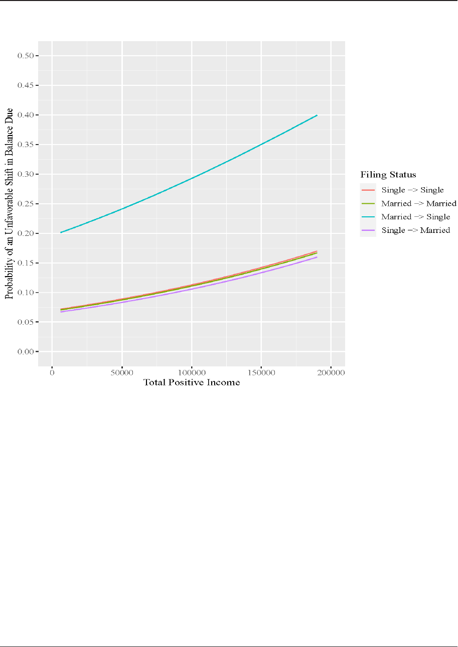
Framinan, Greco, Murphy, Rasey, Alvarez, and Colona
FIGURE
Notes:
Age held constant at median.
An unfavorable shift in balance due is dened as either a change from refund/even to a balance due with or without a CP14 or having a balance due without a CP14 fol-
lowed by a balance due with a CP14.
e impact of divorce on balance due is so large that it completely suppresses the eects of schedule at-
tachment except in one specic circumstance. As shown in Figure , single taxpayers who add a Schedule C
have a higher risk of balance due than divorced taxpayers who add a Schedule C. e dierence in risk be-
tween single and divorced taxpayers who add a Schedule C is small, but noteworthy as the only instance where
divorced taxpayers do not have the highest risk by a substantial margin. We hypothesize that single ling status
may function as a proxy for demographic characteristics associated with workers in the gig economy (i.e.,
younger workers with fewer family ties for whom the gig job is the only source of income). A survey of
gig economy workers
nds that for those whose gig job is the primary source of income, % state it would
be dicult to pay an unexpected expense of ,. For these taxpayers, a balance due on their tax return may
count as an unexpected expense.
8
Gig-Economy-2018-Marketplace-Edison-Research-Poll-FINAL.pdf (edisonresearch.com)

e Balance Due Taxpayer: How Do We Reduce IRS Cost and Taxpayer Burden for Resolving
Balance Due Accounts?
FIGURE
Notes:
Age held constant at median.
An unfavorable shift in balance due is dened as either a change from refund/even to a balance due with or without a CP14 or having a balance due without a CP14 fol-
lowed by a balance due with a CP14.
Schedule C Logistic Regressions
In general, adding Schedule C or having it attached both tax years studied increases the risk of balance due
compared to not having it attached in either year. Figure shows, compared to taxpayers who did not have
Schedule C attached in either TY or TY , the increased risk of adding Schedule C was more than
double and the increased risk for having it attached both years was a little less than double. e eect of add-
ing Schedule C or having it attached both years is not as strong as the impact of divorce; however, the number
of associated returns in these two groups is larger. Approximately million taxpayer returns either added
Schedule C in TY or had it attached in both TY and TY . Of these returns, around . million
(.%) experienced a shi in balance due that resulted with receipt of a CP. e total cost to the IRS for the
CP notices sent to balance due taxpayers who either had Schedule C attached both years or added it in TY
was approximately . million dollars.

Framinan, Greco, Murphy, Rasey, Alvarez, and Colona
FIGURE
Notes:
Age held constant at median.
An unfavorable shift in balance due is dened as either a change from refund/even to a balance due with or without a CP14 or having a balance due without a CP14 fol-
lowed by a balance due with a CP14.
Schedule A Logistic Regressions
As shown in Figure , compared to not having it attached either year, removing Schedule A increased the risk
of a balance due category by a little less than double. Like Schedule C, the increased risk is not as strong as that
of divorce, but it impacts signicantly more taxpayers. Between TY and TY , approximately million
returns dropped Schedule A. Of those, around , (.percent) received a CP, which cost the IRS a little
more than . million dollars.
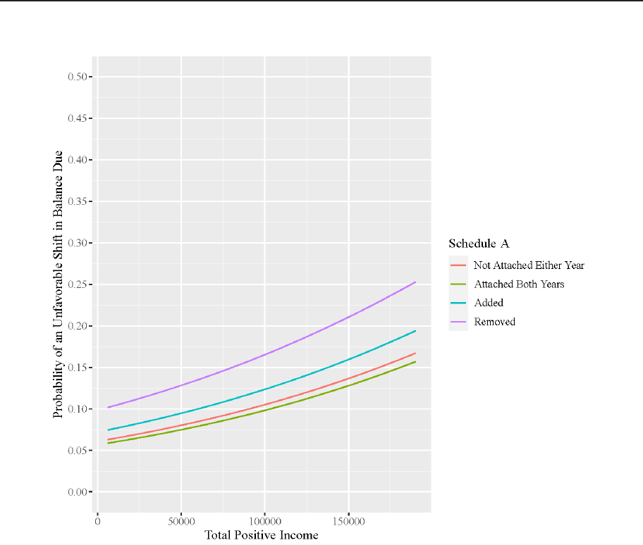
e Balance Due Taxpayer: How Do We Reduce IRS Cost and Taxpayer Burden for Resolving
Balance Due Accounts?
Figure 7. Eect of Schedule A on Balance Due
Notes:
Age held constant at median.
An unfavorable shift in balance due is dened as either a change from refund/even to a balance due with or without a CP14 or having a balance due without a CP14 fol-
lowed by a balance due with a CP14.
Removing Schedule A had a particularly strong impact on single taxpayers. As shown in Figure , remov-
ing Schedule A almost doubled single taxpayers’ risk of a balance due category whereas for other taxpayers
the impact of removing Schedule A was less (for married taxpayers) or nonexistent (for taxpayers who got
married).

Framinan, Greco, Murphy, Rasey, Alvarez, and Colona
FIGURE
Notes:
Age held constant at median.
An unfavorable shift in balance due is dened as either a change from refund/even to a balance due with or without a CP14 or having a balance due without a CP14 fol-
lowed by a balance due with a CP14.
Interaction between divorce and making specic changes to tax returns
As the logistic regression analyses demonstrate, the impact of divorce is large and somewhat independent of
tax return or demographic characteristics like total positive income and age. We conducted crosstab analyses
to further investigate the interactive eect between divorce and specic changes a taxpayer might make to their
tax return during a divorce. e rate at which taxpayers experience an unfavorable balance due shi is %
for taxpayers who get divorced compared to % overall. e impact of additional changes to tax returns does
not dier greatly between all taxpayers and those who get divorced except in two cases. As shown in Figure ,
removing the mortgage interest deduction has a larger additional negative impact on all taxpayers than it does
on taxpayers who get divorced. Similarly, as shown in Figure , having Schedule C attached or adding it has a
larger additional negative impact on all taxpayers than it does on those who get divorced.

e Balance Due Taxpayer: How Do We Reduce IRS Cost and Taxpayer Burden for Resolving
Balance Due Accounts?
FIGURE 9. Percentage of Taxpayers Who Experienced an Unfavorable Balance Due Shift After
Making the Following Changes
FIGURE 10. Percentage of Taxpayers Who Got Divorced and Experienced an Unfavorable
Balance Due Shift After Making the Following Changes
Conclusions
A signicant number of taxpayer (and associated tax return) shis into unfavorable balance due categories is
not due to commonly occurring changes on a taxpayer’s return, such as increased income. Rather, many result
from specic life events associated with ling status, small business activity, and deduction qualications.
Somewhat surprisingly, the nancial impact of an unfavorable shi to balance due is not income specic.
Divorce, removing Schedule A, attaching Schedule C (or having it attached already) aects all income levels
and can happen to any taxpayer. As such, IRS and other stakeholders in the tax administration ecosystem
might consider preemptive mitigation strategies aimed at these groups of taxpayers to reduce the occurrence
of unfavorable balance due positions.

Framinan, Greco, Murphy, Rasey, Alvarez, and Colona
2. Balance Due Gap Analysis
Method
e results of the above statistical analysis make clear that certain groups of taxpayers are particularly vulner-
able to an unfavorable balance due shi: those who get divorced, those who remove Schedule A, and those
who either add Schedule C or attach in both tax years. ese ndings suggest there might be opportunties for
improvement in IRS outreach eorts to ensure taxpayers can easily nd the educational and other resource
materials they need even when not necessarily looking for them. To explore the potential gap, we rst reviewed
current messaging available to taxpayers on IRS.gov. We used specic keywords aected taxpayers might use
to conduct their own research. We chose search terms assuming taxpayers vaguely know divorce or starting a
business has some tax implications. We used the following keywords in the IRS.gov search tool: divorce, start-
ing a small business, and gig economy.
Second, we reviewed current messaging available to taxpayers using the Google search engine. We chose
Google because it controls more than % of the search engine market share worldwide.
We conducted our
Google search of keywords below assuming a naïve taxpayer may not have considered the tax implications of
such life events. We then added the phrase “and taxes” to the end of each keyword/phrase to account for tax-
payers who recognize there are tax implications to certain life events. We used the following keywords/phrases:
• Divorce
9
telanganatoday.com/google-dominates-search-engine-market-holds-92-per-cent-share-report.
10
Small Business Genius.
• Getting divorced
• Starting a new business
• How to start a new
business
• Independent contractor
• Driving for Uber
• Driving for Ly
ird, we conducted an online search for in-person support to capture messaging available to taxpayers
who may not rely on the internet for information. We searched the following groups:
• Divorce attorney organizations
• Divorce support groups
• Tax preparation organizations, CPAs, and accountants
• Tax workshops
We limited our internet searches to the use of an IRS-issued computer. When compared to a similar search
on a non-IRS computer, the results were similar. However, there were dierences in the order results appeared.
Additionally, we limited our Google search to the rst two pages of results. According to an article from Small
Business Genius,
“% of searchers never click past the rst page of results.” So we assume a typical taxpayer
does not likely continue to search internet results beyond page two. We did not include search results marked
“Ad.” In some searches, pages one and two contained minimal information. In such cases, we then proceeded
to page three of the search results.
Results
e search of IRS.gov found several publications and assistance to help meet a taxpayer’s tax obligations
(Appendix A). However, the technical nature of the publications suggest they cater primarily to tax profes-
sionals and those with knowledge of ling taxes. Also, the IRS.gov front page does not specically address the
issue of avoiding a balance due.
Searching the term “divorce” in Google yielded hundreds of results. Most of the webpages surveyed did
not produce results that would help a taxpayer nd information to avoid a balance due situation (Appendix B).

e Balance Due Taxpayer: How Do We Reduce IRS Cost and Taxpayer Burden for Resolving
Balance Due Accounts?
At page two of the search results, we found a government-related website,
which has a link to IRS Publication
, Divorced or Separated Individuals, at IRS.gov. When the keyword phrase included “and taxes,” results
produced several websites oering basic tax advice and included links to divorce attorneys. However, there
were no extensive explanations of taxes related to balance due.
Searching the phrase “starting a new business,” we found basic tax information included in a list of general
advice for those starting a business (Appendix C). Page one contained results with links to the Small Business
Administration
and the U.S. Government website.
Both sites briey discussed ling self-employment taxes
and their related forms. However, neither website contained in-depth information about the potential tax con-
sequences of having a balance due account. Page two of the search results contained a link to the IRS’s Small
Business/Self-Employed webpage. When we added the keyword phrase, “and taxes,” results included more
benecial websites, including IRS.gov.
A search of topics related to the gig economy (Appendix D) and specic companies in the rideshare
industry (e.g., Uber, Ly) produced results with general guidance about working as an independent contrac-
tor. ese companies’ websites contained minimal guidance for meeting tax obligations. Primarily, the sites
emphasized that drivers receive an IRS Form to document income earned and the need to keep accurate
records for tax ling. Searches for “independent contractor” and “gig economy” produced sites with limited
tax advice. Adding the keyword phrase “and taxes” to the initial searches produced links to IRS.gov and sites
with more tax-related topics.
In searching for information about oine tax advice about divorce, starting a business, and working in a
gig economy (see Appendix E), most results were for local support groups and workshops.
Conclusions
A simple Google search on divorce, starting a business, and working in the gig economy provide minimal or
no guidance to naïve taxpayers who may not realize the tax implications of these life events. Searches that add
the phrase “and taxes” produce somewhat more helpful information. However, they do not provide sucient
guidance as an “early intervention.” Taxpayers must know the specic keywords to use to get helpful results.
IRS research has consistently shown individual taxpayers think about taxes and interact with the IRS only
when time to le their tax return. e Taxpayer Experience Survey Free File Focus Groups
found tax-
payers “start thinking about preparing and ling their tax return in late January or early February.” Taxpayers
give little consideration to their potential tax liability earlier in the year. Additionally, Taxpayer Experience
Survey
results indicate % of taxpayers consult only one source for assistance with any tax issues. Finally,
results of the Comprehensive Taxpayer Attitude Survey
show a majority (%) of taxpayers “trust the
IRS to help me understand my tax obligation” and a remarkable % of taxpayers agree “the more information
and guidance the IRS provides, the more likely people are to correctly le their tax returns.” Our ndings sug-
gest IRS attention to early warnings aords a great opportunity to work with partners and stakeholders to ll
the communication and messaging void.
3. Intervention
e results of the two above studies indicate the IRS should review current messaging to encourage taxpayers
(particularly those vulnerable to the balance due shi) to review their tax withholdings, exemptions, etc. im-
mediately upon a signicant life event. e enactment of the Taxpayer First Act
(TFA) in provided the
11
www.benets.gov.
12
www.SBA.gov.
13
www.USA.gov.
14
Internal Revenue Service, Wage and Investment Strategies and Solutions. (July 2020). 2020 Taxpayer Experience Survey (TES) Free File Focus Groups Top Line
Summary Report.
15
Internal Revenue Service, Wage and Investment Strategies and Solutions. (March 2022). Taxpayer Experience Survey (TES) 2021 National Report.
16
Internal Revenue Service, Research, Applied Analytics, and Statistics. (April 2022). Comprehensive Taxpayer Attitude Survey: Past, Present, and Future.
17
Taxpayer First Act | Internal Revenue Service.

Framinan, Greco, Murphy, Rasey, Alvarez, and Colona
IRS an opportunity to reimagine and improve services based on the needs of the taxpayer. Additionally, the
Presidential Executive Order (EO) on Transforming Federal Customer Experience and Service Delivery
to Rebuild Trust in Government
directs Federal agencies to “design and deliver services with a focus on the
actual experience of the people whom it is meant to serve.” To put our ndings to work in service of the TFA
and the EO, WISS and newly formed Taxpayer Experience Oce (TXO) jointly designed data-driven
interventions to help taxpayers avoid the shi to an unplanned balance due.
e TXO formed a Balance Due Team (BDT) to nd proactive solutions to help prevent balance due ac-
counts. Instead of reacting to undesired balance due accounts, taxpayers will employ pre-ling interventions
and strategies to mitigate the underlying causes. is team will collaborate with internal and external stake-
holders to develop, implement, and evaluate plans to reduce the number of taxpayers who have a balance due
at the time of ling. e team aims to accomplish this goal by creating and implementing a phased strategy
divided into three areas of focus:
• Phase 1 (in progress): Divorced taxpayers (change in ling status)
• Phase 2 (tentative): Itemized deductions (Schedule A)
• Phase 3 (tentative): “Side hustle” and gig economy workers (Schedule C)
Since Phase is in progress, we discuss it in detail below.
Phase 1: Divorced Taxpayers
e BDT shares a collective vision to decrease the number of balance due occurrences in divorced taxpayers by
proactively providing education and outreach, services and products, and technology platforms/applications
that meet the needs of the recently divorced taxpayer in the language, timing, and method preferred (choice
and access). e key strategic goals for Phase are as follows.
• Development of IRS.gov/divorce: Information on how divorce can impact taxes is scattered throughout
IRS.gov and can be dicult to nd. As the gap analysis concludes, search engines and the internet have
insucient information readily available. Most sites have little value or a referral to a tax professional for
additional information. e BDT’s goal is to develop IRS.gov/divorce, which will serve as a landing page
for divorced taxpayers and provide a one-stop shop where taxpayers and tax professionals can easily
access divorce related tax material.
• Development of new material: Much of the information on divorce and taxes are in publications and
articles dicult for the average taxpayer to understand. Taxpayers going through a divorce are already
stressed and may abandon their search for relative tax impact information if too dicult. e BDT
seeks to design and develop easy-to-read material to help taxpayers avoid a balance due as they navigate
their divorce. One-page yers such as “How to not owe taxes aer a divorce” or “5 things to know about
divorce and taxes” can grab the attention of a taxpayer going through divorce and provide information
to help them avoid a balance due prior to ling.
• Development of an external communication campaign: e BDT will help create content for external
outreach. e IRS can share this content through social media, online (IRS.gov) and/or directly with
partners. ey will leverage external networks and technology to develop an outreach campaign to drive
trac to IRS.gov/divorce. e IRS can distribute easy-to-understand content on social media posts
across multiple platforms and in multiple languages and otherwise share the new BDT material with
external stakeholders.
18
Executive Order on Transforming Federal Customer Experience and Service Delivery to Rebuild Trust in Government | e White House.

e Balance Due Taxpayer: How Do We Reduce IRS Cost and Taxpayer Burden for Resolving
Balance Due Accounts?
Follow-on Eorts
A foundation of the BDT intervention plan is the WISS statistical analysis and gap analysis that inform eorts
reaching the recently divorced taxpayer, the taxpayer who lost itemized deductions, and the taxpayer with a
“side hustle” or working in the gig economy. Starting in summer , WISS and the BDT leveraged focus
groups with tax preparers at the IRS Nationwide Tax Forums and Latino Tax Fest that gather further input to
support and rene the BDT’s intervention strategy. Tax preparers are a valuable IRS partner and their exten-
sive knowledge regarding the tax-specic information, resources and support taxpayers need to meet their tax
obligations promise to provide valuable insight.

Framinan, Greco, Murphy, Rasey, Alvarez, and Colona
Appendix A. Search Results from IRS.gov
Search
term(s)
Results Comments
Divorce Page 1. “What You Need to Know Before Getting a
Divorce.” https://www.nolo.com/legal-encyclopedia/
getting-started-with-your-divorce.html (retrieved
7/8/2022)
Looked like it would be useful, but when clicked there
was no information on taxes.
Page 1. https://www.ndlaw.com/family/divorce/how-
to-divorce.html (retrieved 7/8/2022)
>>> Followed link on page: https://www.ndlaw.com/
family/divorce/marriage-divorce-taxes-and-your-
social-security-number.html (retrieved 7/8/2022)
Page focused on changing one’s name with SSA af-
ter divorce. No information on taxes; the page recom-
mends contacting a divorce attorney. Page provides
attorney referral service based on Zip Code.
Page 3. https://www.hg.org/divorce-law-center.html.
(Retrieved 7/11/2022)
>>> Followed link to “Divorce Law Basics.”
https://www.hg.org/divorce-law-center.html (retrieved
7/11/2022)
Provides basic information about divorce. No infor-
mation on taxes. Page provides attorney referrals.
Getting
divorced
Page 1. “What Happens in a Divorce?” https://www.
alllaw.com/articles/family/divorce/article64.asp (re-
trieved 7/11/2022). IRS laptop
Provides information on the process of divorce. No
tax considerations given.
Page 1. “Divorce Advice Every Woman Getting a
Divorce Needs To Hear.” https://www.brides.com/
pieces-of-divorce-advice-for-women-1102751 (re-
trieved 7/11/2022)
Recommends gathering nancial information related
to assets and liabilities. No discussion of taxes.
Page 1. “Should I Get a Divorce?” https://www.oprah-
daily.com/life/a26040141/should-i-get-a-divorce/
(retrieved 7/11/2022)
From Oprah Winfrey’s website. Because of her
notoriety and reach, though it would contain useful
information. Site contains “signs” that it is time for
divorce. No tax information provided.
Page 2. https://myguidance.delity.com/ftgw/pna/
public/lifeevents/content/divorce/getting-divorced
(retrieved 7/11/2022)
>>> Clicked link on page “Finances after Divorce.”
https://myguidance.delity.com/ftgw/pna/public/
lifeevents/content/divorce/divorce-and-nances
Website states to “to consider any tax consequences
associated with selling investments in a taxable ac-
count.” No further information provided.
Page 2. “12 Mistakes to Avoid When Divorcing Over
50.” https://www.investopedia.com/personal-nance/
mistakes-avoid-when-divorcing-over-50/ (retrieved
7/11/2022)
Contains a warning not to ignore tax consequences.
Information is about the implications of making/re-
ceiving alimony and child support payments. Refers
the reader to www.benets.gov.
>>> Clicked hyperlink on page “program can help
you” Tax Relief for Divorced or Separated Individu-
als. https://www.benets.gov/benet/946 (retrieved
7/12/2022).
Benets.gov links to Pub 504 at IRS.gov.
Page 2. What Older Adults Should Know about Get-
ting Divorced and (Maybe) Remarried. https://www.
kiplinger.com/personal-nance/604696/what-older-
adults-should-know-about-getting-divorced-and-
maybe-remarried (retrieved 7/11/2022)
Seemed like it would be useful. Contained no infor-
mation on taxes.

e Balance Due Taxpayer: How Do We Reduce IRS Cost and Taxpayer Burden for Resolving
Balance Due Accounts?
Appendix A (continued). Search Results from IRS.gov
Search
term(s)
Results Comments
Page 3. “Divorce.” https://www.legalzoom.com/ar-
ticles/divorce (retrieved 7/11/2022)
>>> Followed link “Considering Divorce? 10 Things to
Think About” https://www.legalzoom.com/articles/con-
sidering-divorce-10-things-to-think-about (retrieved
7/12/2022)
Thought it could have useful information, but it only
contained articles on how to le for divorce and
forms need to le for divorce. No discussion of tax
implications.
Page 3. “Getting Divorced.” https://turbotax.intuit.
com/tax-tips/marriage/getting-divorced/L20NC66cf
(retrieved 7/11/2022)
Good explanation of ling status, claiming depen-
dents, medical expenses, tax credits, payments to
an ex-spouse, transfer of assets, home sale, and
transfer of retirement assets.
Getting
divorced and
taxes
Page 1. Divorce & Taxes 101: Filing Taxes After a Di-
vorce. https://blog.turbotax.intuit.com/tax-tips/divorce-
and-taxes-4018/ (retrieved 7/22/2022)
Brief discussion about ling status, claiming child
support, requirement for ling as HOH, Child and De-
pendent Care credit. The article is followed by people
posting their questions, comments. Most recent post
was from 2018.
Page 1. Filing Taxes After Divorce: A Practical Guide.
https://smartasset.com/taxes/ling-taxes-after-divorce
(retrieved 7/22/2022)
Advice on choosing the right ling status, updating
one’s W-4, claiming dependents, and deducting legal
fees.
Page 1. Most-Overlooked Tax Breaks for the Newly
Divorced. https://www.kiplinger.com/taxes/tax-deduc-
tions/602038/most-overlooked-tax-breaks-for-the-
newly-divorced (retrieved 7/22/2022)
Reminds taxpayers to update W-4, how to determine
if one qualies for ling as HOH, alimony payments
for divorce decrees before end of 2018. Noncustodial
parents must complete Form 8332 if they claim child
tax credit.
Page 1. Filing Taxes After Divorce. https://www.
hrblock.com/tax-center/ling/personal-tax-planning/
divorce-and-taxes/ (retrieved 7/22/2022)
Alimony payments no longer deductible. Refers
taxpayers to Form 8332 noncustodial parent claiming
the child/children. Discusses how IRAs are handled.
Page 1. Tax Complications to Watch Out for During
and After a Divorce. https://familylaw.lyttlelaw.com/
tax-complications-to-watch-out-for-during-and-after-a-
divorce.html (retrieved 7/22/2022)
Austin, TX, divorce attorney page. Explains how to
divide tax refunds, ling tax returns in TX, require-
ment for ling HOH.
Page 1. What Getting Divorced or Separated Means
for Your 2021 Tax Return. https://www.thebalance.
com/what-divorced-or-separated-means-for-tax-
es-4125740 (retrieved 7/22/2022)
Divorce must be nal before end of year for IRS to
recognize. Refers to Pub 504; ling as HOH; claiming
the children; alimony no longer deductible; paying
back taxes and property taxes.
Page 1. Your Taxes After Divorce. https://www.
investopedia.com/taxes-after-divorce-5192868 (re-
trieved 7/22/2022)
Discusses ling status and qualifying for HOH.
Explains rules related to Earned Income Credit,
American Opportunity Tax Credit, and child and
dependent care credit. After 2018 alimony payments
were no longer deducted from taxable income. Gains
on the sale of primary home not taxable up to $250K;
claiming HOH.
Page 2. Tax Tips for Women Going Through Divorce.
https://www.forbes.com/sites/jeanders/2012/03/07/
tax-tips-for-women-going-through-divorce/ (retrieved
7/22/2022)
Warns about ling joint returns, how to handle over/
underpayments, ling HOH, claiming children, child
support and alimony considerations, capital gains tax
on high ticket assets held for a long time

Framinan, Greco, Murphy, Rasey, Alvarez, and Colona
Appendix B. Internet Search Results for “Divorce” Topics
Search
term(s)
Results Comments
Divorce Page 1. “What You Need to Know Before Getting a
Divorce.” https://www.nolo.com/legal-encyclopedia/
getting-started-with-your-divorce.html (retrieved
7/8/2022).
Looked like it would be useful, but when clicked there
was no information on taxes.
Page 1. https://www.ndlaw.com/family/divorce/how-
to-divorce.html (retrieved 7/8/2022).
>>> Followed link on page: https://www.ndlaw.com/
family/divorce/marriage-divorce-taxes-and-your-
social-security-number.html (retrieved 7/8/2022).
Page focused on changing one’s name with SSA
after divorce. No information on taxes; the page
recommends contacting a divorce attorney. Page
provides attorney referral service based on Zip Code
Page 3. https://www.hg.org/divorce-law-center.html
(Retrieved 7/11/2022).
>>> Followed link to “Divorce Law Basics.”
https://www.hg.org/divorce-law-center.html (retrieved
7/11/2022).
Provides basic information about divorce. No infor-
mation on taxes. Page provides attorney referrals.
Getting
divorced
Page 1. “What Happens in a Divorce?” https://www.
alllaw.com/articles/family/divorce/article64.asp (re-
trieved 7/11/2022). IRS laptop.
Provides information on the process of divorce. No
tax considerations given.
Page 1. “Divorce Advice Every Woman Getting a
Divorce Needs To Hear.” https://www.brides.com/
pieces-of-divorce-advice-for-women-1102751 (re-
trieved 7/11/2022).
Recommends gathering nancial information related
to assets and liabilities. No discussion of taxes.
Page 1. “Should I Get a Divorce?” https://www.oprah-
daily.com/life/a26040141/should-i-get-a-divorce/
(retrieved 7/11/2022).
From Oprah Winfrey’s website. Because of her
notoriety and reach, though it would contain useful
information. Site contains “signs” that it is time for
divorce. No tax information provided.
Page 2. https://myguidance.delity.com/ftgw/pna/
public/lifeevents/content/divorce/getting-divorced
(retrieved 7/11/2022).
>>> Clicked link on page “Finances after Divorce.”
https://myguidance.delity.com/ftgw/pna/public/
lifeevents/content/divorce/divorce-and-nances
Website states to “to consider any tax consequences
associated with selling investments in a taxable ac-
count.” No further information provided.
Page 2. “12 Mistakes to Avoid When Divorcing Over
50.” https://www.investopedia.com/personal-nance/
mistakes-avoid-when-divorcing-over-50/ (retrieved
7/11/2022).
Contains a warning not to ignore tax consequences.
Information is about the implications of making/re-
ceiving alimony and child support payments. Refers
the reader to www.benets.gov
>>> Clicked hyperlink on page “program can help
you” Tax Relief for Divorced or Separated Individu-
als. https://www.benets.gov/benet/946 (retrieved
7/12/2022).
Benets.gov links to Pub 504 at IRS.gov.
Page 2. What Older Adults Should Know about Get-
ting Divorced and (Maybe) Remarried. https://www.
kiplinger.com/personal-nance/604696/what-older-
adults-should-know-about-getting-divorced-and-
maybe-remarried (retrieved 7/11/2022).
Seemed like it would be useful. Contained no infor-
mation on taxes.

e Balance Due Taxpayer: How Do We Reduce IRS Cost and Taxpayer Burden for Resolving
Balance Due Accounts?
Appendix B (continued). Internet Search Results for “Divorce” Topics
Search
term(s)
Results Comments
Page 3. “Divorce.” https://www.legalzoom.com/ar-
ticles/divorce (retrieved 7/11/2022).
>>> Followed link “Considering Divorce? 10 Things
to Think About.” https://www.legalzoom.com/articles/
considering-divorce-10-things-to-think-about (re-
trieved 7/12/2022).
Thought it could have useful information, but it only
contained articles on how to le for divorce and
forms need to le for divorce. No discussion of tax
implications.
Page 3. “Getting Divorced.” https://turbotax.intuit.
com/tax-tips/marriage/getting-divorced/L20NC66cf
(retrieved 7/11/2022).
Good explanation of ling status, claiming depen-
dents, medical expenses, tax credits, payments to
an ex-spouse, transfer of assets, home sale, and
transfer of retirement assets.
Getting
divorced and
taxes
Page 1. Divorce & Taxes 101: Filing Taxes After a Di-
vorce. https://blog.turbotax.intuit.com/tax-tips/divorce-
and-taxes-4018/ (retrieved 7/22/2022).
Brief discussion about ling status, claiming child
support, requirement for ling as HOH, Child and De-
pendent Care credit. The article is followed by people
posting their questions, comments. Most recent post
was from 2018.
Page 1. Filing Taxes After Divorce: A Practical Guide.
https://smartasset.com/taxes/ling-taxes-after-divorce
(retrieved 7/22/2022).
Advice on choosing the right ling status, updating
one’s W-4, claiming dependents, and deducting legal
fees.
Page 1. Most-Overlooked Tax Breaks for the Newly
Divorced. https://www.kiplinger.com/taxes/tax-deduc-
tions/602038/most-overlooked-tax-breaks-for-the-
newly-divorced (retrieved 7/22/2022).
Reminds taxpayers to update W-4, how to determine
if one qualies for ling as HOH, alimony payments
for divorce decrees before end of 2018. Noncustodial
parents must complete Form 8332 if they claim child
tax credit.
Page 1. Filing Taxes After Divorce. https://www.
hrblock.com/tax-center/ling/personal-tax-planning/
divorce-and-taxes/ (retrieved 7/22/2022).
Alimony payments no longer deductible. Refers
taxpayers to Form 8332 noncustodial parent claiming
the child/children. Discusses how IRAs are handled.
Page 1. Tax Complications to Watch Out for During
and After a Divorce. https://familylaw.lyttlelaw.com/
tax-complications-to-watch-out-for-during-and-after-a-
divorce.html (retrieved 7/22/2022)
Austin, TX, divorce attorney page. Explains how to
divide tax refunds, ling tax returns in TX, require-
ment for ling HOH.
Page 1. What Getting Divorced or Separated Means
for Your 2021 Tax Return. https://www.thebalance.
com/what-divorced-or-separated-means-for-tax-
es-4125740 (retrieved 7/22/2022).
Divorce must be nal before end of year for IRS to
recognize. Refers to Pub 504; ling as HOH; claiming
the children; alimony no longer deductible; paying
back taxes and property taxes.
Page 1. Your Taxes After Divorce. https://www.
investopedia.com/taxes-after-divorce-5192868 (re-
trieved 7/22/2022).
Discusses ling status and qualifying for HOH.
Explains rules related to Earned Income Credit (EIC),
American Opportunity Tax Credit (AOTC), and child
and dependent care credit. After 2018 alimony pay-
ments were no longer deducted from taxable income.
Gains on the sale of primary home not taxable up to
$250K; claiming HOH.
Page 2. Tax Tips for Women Going Through Divorce.
https://www.forbes.com/sites/jeanders/2012/03/07/
tax-tips-for-women-going-through-divorce/ (retrieved
7/22/2022).
Warns about ling joint returns, how to handle over/
underpayments, ling HOH, claiming children, child
support and alimony considerations, capital gains tax
on high ticket assets held for a long time.
Page 2. Divorced or Separated and Income Taxes.
https://www.ele.com/divorce-or-separated-and-
taxes/ (retrieved 7/22/2022).
Discusses ling status as HOH, enrolling in health
insurance plan and calculating Premium Tax Credit,
retirement contributions, handling alimony and child
support.

Framinan, Greco, Murphy, Rasey, Alvarez, and Colona
Appendix C. Internet Search Results for “Starting a New Business” Topics
Search
term(s)
Results Comments
Starting a new
business
Page 1. How to Start a Business: A Step-by-Step
Guide. https://www.businessnewsdaily.com/4686-
how-to-start-a-business.html (retrieved 7/13/2022).
Looked like it would have benecial information. Only
mentioned how to apply for an EIN and register busi-
ness with the state. No discussion of paying taxes.
Page 1. 10 steps to start your business. https://www.
sba.gov/business-guide/10-steps-start-your-business
(retrieved 7/13/2022).
Thought a government website would have informa-
tion on paying taxes. The site explains how to apply
for an EIN with IRS and how to get a state tax ID
number, but no mention of paying taxes.
Page 1. Start Your Own Business. https://www.usa.
gov/start-business (retrieved 7/13/2022).
Thought a government website would have informa-
tion on paying taxes. The site explains how to apply
for an EIN with IRS and how to get a state tax ID
number, but no mention of paying taxes.
Page 1. How To Start A Small Business In 2022:
Complete Step-By-Step Guide. https://www.forbes.
com/advisor/business/how-to-start-a-business/
(retrieved 7/13/2022).
One paragraph explaining that it is important to start
planning for taxes—income, self-employment, etc.
No other mention of paying taxes.
Page 1. How to Start a Business in 13 Steps. https://
www.nerdwallet.com/article/small-business/how-to-
start-a-business (retrieved 7/13/2022).
Has a section with links to other tax-related articles.
>>>Followed link A Tax Guide for Small-Business
Owners. https://www.nerdwallet.com/article/small-
business/small-business-tax-preparation (retrieved
7/13/2022).
Brief description of Schedule C, Form 1120, Sched-
ule K-1. Recommends contacting a tax professional.
>>>Followed link 15 Self-Employment Tax Deduc-
tions in 2022. https://www.nerdwallet.com/article/
taxes/self-employment-tax-deductions (retrieved
7/13/2022).
Provides a list of potential deductions with refer-
ences to various IRS publications (436—travel
expenses, 535—business expenses)
>>>Followed link How Estimated Quarterly Taxes
Work. https://www.nerdwallet.com/article/taxes/
estimated-quarterly-taxes (retrieved 7/13/2022).
Explains how to calculate and pay estimated taxes
Page 2. The Complete, 12-Step Guide to Start-
ing a Business. https://www.entrepreneur.com/ar-
ticle/297899 (retrieved 7/13/2022).
Looked like it would have benecial information. No
discussion of paying taxes.
Page 2. How to Start a Business From Scratch.
https://www.thehartford.com/business-insurance/
strategy/how-to-start-a-business (retrieved
7/13/2022).
Looked like it would have benecial information. No
discussion of paying taxes.
Page 2. How to Start a Business. https://howtostar-
tanllc.com/start-a-business (retrieved 7/13/2022).
Looked like it would have benecial information. Only
mentioned how to apply for an EIN and register busi-
ness with the state. No discussion of paying taxes.
Page 2. How to Start a Business: A Guide to Starting
a Business. https://www.oberlo.com/blog/how-to-
start-a-business (retrieved 7/13/2022).
General information about starting a business (com-
ing up with a business idea, writing a business plan).
No information about taxes.

e Balance Due Taxpayer: How Do We Reduce IRS Cost and Taxpayer Burden for Resolving
Balance Due Accounts?
Appendix C (continued). Internet Search Results for “Starting a New
Business” Topics
Search
term(s)
Results Comments
Page 2. Checklist for Starting a Business. https://
www.irs.gov/businesses/small-businesses-self-
employed/checklist-for-starting-a-business (retrieved
7/13/2022).
IRS.gov
>>>Followed link Business Taxes. https://www.irs.
gov/businesses/small-businesses-self-employed/
business-taxes (retrieved 7/13/2022).
Explanation of income tax, estimated tax, self-em-
ployment tax, employment taxes
How to start a
small business
Page 1. How to Start a Small Business. https://www.
adp.com/resources/articles-and-insights/articles/h/
how-to-start-a-small-business-a-step-by-step-guide.
aspx (retrieved 7/13/2022).
Contained information on how to apply for an EIN
with the IRS.
>>>Followed link How to Do Payroll. https://www.
adp.com/resources/articles-and-insights/articles/h/
how-to-do-payroll.aspx (retrieved 7/13/2022).
Contained information about calculating payroll taxes
and ling forms 941 (quarterly withholding) and 940
(Federal unemployment tax).
Page 1. How to Start a Business: A Step-by-Step
Guide. https://www.businessnewsdaily.com/4686-
how-to-start-a-business.html (retrieved 7/13/2022).
Looked like it would be benecial. Only mentioned
how to apply for an EIN and register business with
the state. No discussion of paying taxes.
Page 1. How To Start A Small Business In 2022:
Complete Step-By-Step Guide. https://www.forbes.
com/advisor/business/how-to-start-a-business/
(retrieved 7/13/2022).
Thought it would have good information. Only men-
tioned how to apply for an EIN and register business
with the state. No discussion of paying taxes.
Page 2. How to Start a Business. https://howtostar-
tanllc.com/start-a-business (retrieved 7/13/2022).
Thought it would have good information. Only men-
tioned how to apply for an EIN and register business
with the state. No discussion of paying taxes.
Page 2. How to Start a Small Business at Home.
https://www.uschamber.com/co/start/startup/starting-
small-business-at-home (retrieved 7/13/2022).
Thought it would have good information. Only men-
tioned how to apply for an EIN and register business
with the state. Encourages hiring a tax professional.
No discussion of paying taxes.
Page 2. How To Start A Business When You Have
Literally No Money. https://girlboss.com/blogs/
read/start-a-business-without-money (retrieved
7/13/2022).
Female entrepreneur-targeted website. Thought
would have good information. No discussion of
taxes. Only information about how to apply for an
EIN. The site encourages hiring an employment at-
torney. Encourages visiting SBA.gov
Page 2. How to Start a Small Business. https://
www.wikihow.com/Start-a-Small-Business (retrieved
7/13/2022).
Looked like it would be benecial. Only recommend-
ed hiring an accountant or attorney to help with tax
matters. No discussion of paying taxes.
Page 2. How to Grow a Successful Business. https://
www.investopedia.com/articles/pf/08/make-money-
in-business.asp (retrieved 7/13/2022).
Thought the site would have information about
keeping a business in compliance but there was no
information related to taxes.

Framinan, Greco, Murphy, Rasey, Alvarez, and Colona
Appendix C (continued). Internet Search Results for “Starting a New
Business” Topics
Search
term(s)
Results Comments
Starting a
business and
taxes
Page 1. Checklist for Starting a New Business.
https://www.irs.gov/businesses/small-businesses-
self-employed/checklist-for-starting-a-business
(retrieved 7/22/2022).
IRS website with useful information for small busi-
ness owners
Page 1. Starting a Business. https://turbotax.intuit.
com/tax-tips/small-business-taxes/starting-a-busi-
ness/L7PBcAdVh (retrieved 7/22/2022).
Information about choosing an accounting method,
ling quarterly taxes, paying employment taxes,
keeping records for Schedule C, determining whether
taxpayer is an employee or independent contrac-
tor, keeping track of expenses, and home oce
deductions
Page 1. Small Business Tax Information. https://www.
usa.gov/business-taxes (retrieved 7/22/2022).
Government website with link to back to IRS.gov
Page 1. Tax and Business Forms You’ll Need to Start
a Small Business. https://www.businessnewsdaily.
com/9-tax-and-business-forms-needed-to-start-a-
small-business.html (retrieved 7/22/2022).
Contained guidance on paying estimated taxes, pay-
ing employment taxes if a company has employees,
completing tax Form Schedule C, and information
about business tax deductions.

e Balance Due Taxpayer: How Do We Reduce IRS Cost and Taxpayer Burden for Resolving
Balance Due Accounts?
Appendix D. Internet Search Results for “Gig Economy” Topics
Search
term(s)
Results Comments
Driving for
Uber
Page 1. Flexible driving opportunities with Uber.
https://www.uber.com/us/en/drive/ (retrieved
.7/14/2022)
Main recruiting page for Uber. Describes benets of
driving with the company. No information about taxes.
Page 1. Uber Driver Requirements: A Step-by-Step
Guide. https://www.investopedia.com/articles/per-
sonal-nance/120315/how-become-uber-driver-step-
step-guide.asp (retrieved 7/14/2022).
Subheading “How Do Uber Drivers Pay Taxes?” Ex-
plains self-employment tax rate of 15.3% (Medicare
and SS). Advises to talk with a CPA about what can
be written o as expenses.
Page 1. I’m a driver for Uber and Lyft — here are 10
things I wish I knew before starting the job. https://
www.businessinsider.com/uber-lyft-drivers-job-ad-
vice-car-2019-8 (retrieved 7/14/2022).
Looked like it would be helpful but did not mention
anything about taxes or tax planning.
Page 1. How to Become an Uber Driver: A Beginner’s
Guide. https://www.nerdwallet.com/article/nance/
how-to-become-an-uber-driver (retrieved 7/14/2022).
Reminds gig workers that they are responsible for
12.4% to Social Security and 2.9% to Medicare, for a
total of 15.3%
>>> Followed link to “What Gig Workers Need to
Know About Taxes.” https://www.nerdwallet.com/
article/nance/what-gig-workers-need-to-know-about-
taxes (retrieved 7/14/2022).
Brief mention of deducting retirement plan
contributions.
Warns about underpayment penalties. Encourages
setting up a payment plan if one cannot aord to pay
their taxes.
Page 2. Is Driving for Uber Worth It in 2022? https://
millennialmoneyman.com/driving-for-uber/ (retrieved
7/14/2022).
Brief comment about self-employment taxes. Encour-
ages downloading mileage tracking applications.
Page 2. Make Money Driving For Uber: The Ultimate
Side Hustle. https://www.goodnancialcents.com/
how-to-become-an-uber-driver-requirements/ (re-
trieved 7/14/2022).
Reminds drivers they are responsible for (1) their
tax bill, including paying quarterly tax payments if
applicable; (2) keeping track the mileage; and (3) col-
lecting receipts for gas and vehicle upkeep.
Page 2. How Much Do Uber Drivers Make? Is It
Worth Your Time? https://www.gobankingrates.com/
money/side-gigs/how-much-do-uber-drivers-make/
(retrieved 7/14/2022).
Informs drivers they will need to pay self-employment
taxes.
>>> Followed link to How Does an Independent Con-
tractor Pay Taxes? https://www.gobankingrates.com/
taxes/ling/independent-contractor-taxes/ (retrieved
7/14/2022).
Talks about self-employment taxes.
>>> Followed link to Got a Side Hustle? Here’s How
To Calculate Estimated Taxes. https://www.gobank-
ingrates.com/taxes/ling/deadline-countdown-self-
employment-guide-ling/ (retrieved 7/14/2022).
Explains when and how to le quarterly estimated
taxes.
Driving for Lyft Page 1. It pays (a lot) to drive right now. https://www.
lyft.com/drive-with-lyft (retrieved 7/14/2022).
Main recruiting page for Lyft. Describes benets
of driving with the company. No information about
taxes.

Framinan, Greco, Murphy, Rasey, Alvarez, and Colona
Appendix D (continued). Internet Search Results for “Gig Economy” Topics
Search
term(s)
Results Comments
Page 1. How much can you make driving for Lyft in
Atlanta? https://www.quora.com/How-much-can-you-
make-driving-for-Lyft-in-Atlanta (retrieved 7/14/2022).
Discussion board about driving for Lyft
>>>Searched in Quora “Lyft+Taxes.” https://www.
quora.com/search?q=lyft%20taxes (retrieved
7/14/2022).
General information about taxes. Most post refer the
reader to IRS.gov
Page 2. How Much Do Lyft Drivers Make? https://
www.gobankingrates.com/money/side-gigs/how-
much-do-lyft-drivers-make/ (retrieved 7/14/2022).
Thought the site would have information regarding
ling and reporting taxes related to earnings. No
information about taxes.
Page 2. Your Step-By-Step Guide to Becoming a Lyft
Driver [2022 Update]. https://www.ridester.com/drive-
for-lyft/ (retrieved 7/14/2022).
Site oers information only on how to initially get set
up with Lyft. No information about taxes.
Page 2. Lyft vs. Uber: What’s the Dierence?
https://www.investopedia.com/articles/personal--
nance/010715/key-dierences-between-uber-and-lyft.
asp (retrieved 7/14/2022).
Thought this would have information since it ap-
peared under Investopedia’s “Personal Finance”
section. No information about taxes.
>>>Followed link to “Gig Economy” https://www.
investopedia.com/terms/g/gig-economy.asp (retrieved
7/14/2022).
Provides basic information about the gig economy.
No information about taxes.
Page 2. How to Become a Lyft Driver. https://gigwork-
er.com/become-lyft-driver/ (retrieved 7/14/2022).
Site oers information only on how to initially get set
up with Lyft. No information about taxes.
Gig Economy Page 1. Gig Economy. https://www.investopedia.com/
terms/g/gig-economy.asp (retrieved 7/14/2022).
Provides basic information about the gig economy.
No information about taxes.
Page 1. Thriving in the Gig Economy. https://hbr.
org/2018/03/thriving-in-the-gig-economy (retrieved
7/14/2022).
Provides general information. No mention of taxes.
Page 2. What is the gig economy and what’s the
deal for gig workers? https://www.weforum.org/agen-
da/2021/05/what-gig-economy-workers/ (retrieved
7/14/2022).
Provides a denition of the gig economy. No informa-
tion about taxes.
What is the Gig Economy? The Complete Guide for
2022. https://www.oberlo.com/blog/what-is-the-gig-
economy (retrieved 7/14/2022).
Provides pros and cons to the gig economy. No infor-
mation about taxes.
Independent
Contractor
Page 1. Independent Contractor (Self-Employed) or
Employee? https://www.irs.gov/businesses/small-
businesses-self-employed/independent-contractor-
self-employed-or-employee (retrieved 7/14/2022).
IRS.gov. See IRS search results.
Page 1. Independent Contractor. https://www.
investopedia.com/terms/i/independent-contractor.asp
(retrieved 7/14/2022).
Provides independent contractor information about
their self-employment tax responsible for Social
Security and Medicare.
Brief mention of deducting retirement plan
contributions.
Lists common tax forms for independent contractors
(Schedule C, 1040, 1040-ES)

e Balance Due Taxpayer: How Do We Reduce IRS Cost and Taxpayer Burden for Resolving
Balance Due Accounts?
Appendix D (continued). Internet Search Results for “Gig Economy” Topics
Search
term(s)
Results Comments
Page 1. Minimum Requirements for Working as an
Independent Contractor https://www.nolo.com/legal-
encyclopedia/minimum-requirements-working-inde-
pendent-contractor-29978.html (retrieved 7/14/2022).
A section of the article describes registering for an
EIN with IRS and completing a Schedule C.
Page 1. Understanding What an Independent Con-
tractor Is. https://www.businessnewsdaily.com/15853-
independent-contractor-employee-dierences.html
(retrieved 7/14/2022).
Describes the denition of an independent contractor.
No information about ling taxes.
Page 1. Employee or Independent Contractor? UGA.
https://www.georgiasbdc.org/employee-or-indepen-
dent-contractor/ (retrieved 7/14/2022).
Describes the IRS denition of an independent
contractor and refers the reader to Pub 15a (link was
broken http://www.irs.gov/pub/irs-pdf/p15a.pdf)
Also refers readers to SBA for a denition of indepen-
dent contractor.
No tax information provided.
Page 2. What is an Independent Contractor? https://
andersonadvisors.com/independent-contractor/
(retrieved 7/14/2022).
Explains that independent contractors have to pay
their own Social Security taxes. Explains the require-
ments for issuing 1099s
Page 2. Fair Labor Standards Act Advisor—Indepen-
dent Contractor. https://webapps.dol.gov/elaws/whd/
sa/docs/contractors.asp (retrieved 7/14/2022).
DOL.gov. Denes an independent contractor. No tax
information provided.
Page 2. What Is An Independent Contrac-
tor? Here’s Why It Matters Under the Trump
Tax Law. https://www.forbes.com/sites/alan-
gassman/2018/10/05/what-is-an-independent-
contractor/?sh=37b9c2871692 (retrieved 7/14/2022).
Describes the IRS “Pass Through Deduction” (Tax
Cuts and Jobs Act). No information about ling taxes.
Driving for
Uber and
taxes
Page 1. How Do Rideshare (Uber and Lyft) Drivers
Pay Taxes? https://www.taxoutreach.org/rideshare/
how-do-rideshare-uber-and-lyft-drivers-pay-taxes-2/
(retrieved 7/22/2022).
Discussed self-employment taxes, tracking deduc-
tions, ling quarterly taxes, and completing a Sched-
ule C and Schedule SE.
Page 1. Tax Deductions for Rideshare (Uber and Lyft)
Drivers and Food Couriers. https://www.taxoutreach.
org/rideshare/tax-deductions-for-rideshare-uber-and-
lyft-drivers/ (retrieved 7/22/2022).
Explains standard vehicle deductions and provided
an infographic on choosing the Standard Mileage
Deduction vs. Actual Expenses. The site provides a
sample of a 1099 and how to complete a Schedule C.
Page 1. Tax Tips for Uber Driver-Partners: Under-
standing Your Taxes. https://turbotax.intuit.com/tax-
tips/self-employment-taxes/tax-tips-for-uber-drivers-
understanding-your-taxes-/L7sbLCSc4 (retrieved
7/22/2022).
Contains information on 1099s, being self-employed,
completing Schedule C, deducting mileage, and ex-
amples of other tax-deductible business expenses.
Page 1. Your tax questions, answered https://www.
uber.com/us/en/drive/tax-information/ (retrieved
7/22/2022).
Provides a brief explanation of tax documents and
promotes the use of TurboTax.
Page 1. The Uber & Lyft Driver’s Guide to Taxes
https://bench.co/blog/tax-tips/uber-driver-taxes/
(retrieved 7/22/2022).
Discusses self-employment taxes, ling quarterly
estimates, and completing Schedule C. Oers a
subscription service to maintain tax records.

Framinan, Greco, Murphy, Rasey, Alvarez, and Colona
Appendix D (continued). Internet Search Results for “Gig Economy” Topics
Search
term(s)
Results Comments
Page 2. 5 Things to Know About Rideshare
Driver Taxes https://www.morningbrew.com/daily/
stories/2021/04/22/5-things-know-rideshare-driver-
taxes (retrieved 7/22/2022).
Explains Form 1099, the concept of “ordinary and
necessary,” vehicle deductions, and the Qualied
Business Income (QBI) deduction.
Page 2. Tax Tips for Lyft and Uber Drivers: What to
Know for 2021. https://www.picnictax.com/blog/lyft-
uber-rideshare-driver-taxes/ (retrieved 7/22/2022).
Contains information on 1099s, being self-employed,
completing Schedule C, and deducting mileage.
Page 3. Uber Tax Information: Essential Tax Forms,
Documents, & Checklists. https://www.ridester.com/
uber-tax-information/ (retrieved 7/22/2022).
Discussed self-employment taxes, tracking deduc-
tions, ling quarterly taxes, and completing a Sched-
ule C and Schedule SE.
Page 3. Learn How to File Taxes for Uber and Lyft
Drivers https://www.udemy.com/course/learn-how-to-
le-taxes-from-uber-lyft/ (retrieved 7/22/2022).
Oers a course for $39.99 on how to le taxes for
Uber and Lyft drivers.
Page 3. Taxes for Rideshare/Uber Drivers https://
www.solvable.com/tax-help/business-taxes/taxes-for-
rideshare-uber-drivers/ (retrieved 7/22/2022).
Provides information on acting as an independent
contractor, ling appropriate tax forms, completing
Schedules C and SE, ling quarterly estimated taxes.

e Balance Due Taxpayer: How Do We Reduce IRS Cost and Taxpayer Burden for Resolving
Balance Due Accounts?
Appendix E. Search Results for Oine Resources
Search
term(s)
Results Comments
Divorce sup-
port groups
Page 1. Divorce Support Groups—Atlanta
https://www.psychologytoday.com/us/groups/ga/
atlanta?category=divorce (retrieved 7/18/2022).
Support group and psychologist referrals service.
Page 1. Oasis—Buckhead Church—Divorce Re-
covery https://buckheadchurch.org/oasis (retrieved
7/18/2022).
Atlanta-based church that oers divorce support
groups.
Divorce
attorney
organizations
Page 1. American Academy of Matrimonial Lawyers.
https://www.aaml.org/ (retrieved 7/18/2022).
>>>Searched AAML Journal “taxes.” Article: Divorce
and Taxes: Fifty Years of Change Volume 24,
2012, Number 2, p. 489 https://aaml.org/resource/
collection/3BDEDFA9-B18B-4C53-B875-2CF630D-
DAD9C/Wilder.pdf (retrieved 7/18/2022).
Article discussing ling status rules.
Divorce
workshops
Page 1. Second Saturday. https://www.secondsatur-
day.com/ (retrieved 7/19/2022).
>>>Click “Find a Workshop”
>>>Choose State
Provides a list of online in-person workshops for
divorced people.
Page 1. Family Law Workshop Information https://
www.fultoncourt.org/family/family-workshop.php
(retrieved 7/19/2022).
Fulton County (Georgia) Court provides workshops
for people going through/considering divorce.
Tax advice
for small
businesses
No valuable results
Tax
workshops
Page 1. Small Business Tax Workshops, Meetings
and Seminars https://www.irs.gov/businesses/small-
businesses-self-employed/small-business-tax-work-
shops-meetings-and-seminars (retrieved 7/19/2022).
IRS.gov website. Taxpayer chooses their state for a
list of tax workshops in their area.
Page 1. TaxworkShop.com. https://www.taxworkshop.
com/ (retrieved 7/19/2022).
Workshops for tax practitioners. Last scheduled
workshop was September 2021.
Gig economy
workshops
No valuable results.

e Impact of Annual Changes in Family
Structure and Income on Tax Credits
Elaine Maag, Nikhita Airi, and Lillian Hunter (Urban-Brookings Tax Policy Center)
1
I. Introduction
Refundable tax credits, those that can exceed federal income taxes owed, provide an important source of -
nancial support for many low- and middle-income families with children. e largest of these are the Earned
Income Tax Credit (EITC) and Child Tax Credit (CTC). e credits are determined on an annual basis and
are oen received as a single payment as part of a family’s tax refund. For low-income families, it is oen the
family’s most signicant nancial event of the year (Morduch and Schneider ()).
Tax credits accrue to tax units—the group of individuals who appear on a tax return together based on
legal relationships, child residency, and support. ough families may change throughout the year, only one
adult or married couple will likely be able to benet from the EITC and CTC for any one child (and oen it is
the same person for both credits), even when several adults provide signicant amounts of support to a child
throughout the year.
Because most families le taxes once a year, aer the tax year has ended, families that change throughout
the year may have diculties correctly determining their ling status and who can properly claim a child for
the purpose of receiving child-related benets. According to the Internal Revenue Service (IRS), the most
common error lers make when claiming the EITC is claiming a child who is not actually a qualifying child
(IRS ()).
Families oen report that the amount of tax credits they receive at tax time are a surprise (T. Anderson et
al. (); Romich and Weisner ()). e complexity of the credits along with family and income changes
throughout the year may contribute to not knowing what credits are likely to be delivered at tax time (Maag et
al. (); Maag et al. ()).
is analysis reviews how trends in changing family structures diverge from how tax credits are delivered.
We then briey describe the EITC and CTC and the role income and family composition play in their calcula-
tions. Finally, we explore how well data in one year predict EITC and CTC receipt in a subsequent year.
Understanding the predictability of tax credits is important for two reasons. First, because the EITC and
CTC are signicant sources of economic support for families, it is important to gain a better understanding of
how much credit amounts vary from year to year. Second, recent experience with advancing up to half of the
CTC in has re-energized calls for delivering tax credits on a monthly basis in advance of families ling a
tax return.
If credits are advanced based on information from the prior year, families that experience drops in credits
for which they are eligible may be required to repay any credit they received in error when they complete their
tax return. is may create a hardship for some families. Uncertainty about tax credits can cause tax lers to
1
is brief was funded by Intuit Financial Freedom Foundation and the Annie E. Casey Foundation through the Innovations in Cash Assistance for Children
initiative. e authors are grateful to them and to all our funders, who make it possible for the Urban-Brookings Tax Policy Center to advance its mission.
e views expressed are those of the authors and should not be attributed to the Urban-Brookings Tax Policy Center, the Urban Institute, the Brookings Institution,
their trustees, or their funders.
e authors gratefully thank Joyce Morton, who developed and created the datasets underlying this analysis, Kevin Werner, who performed microsimulation
modeling runs, and Laura Wheaton who advised the construction of the analysis le and reviewed an earlier dra of the paper. We also thank Donald Marron,
Tracy Gordon, Krista Holub, and Charlie Leonard for thoughtful comments on an earlier dra, Alexandria Dallman for editorial review, and Muskan Jha for
publication support. TRIM3 is maintained and developed by the Urban Institute, under primary funding from the Department of Health and Human Services,
Oce of the Assistant Secretary for Planning and Evaluation (HHS/ASPE).

Maag, Airi, and Hunter
take unnecessary precautions, such as borrowing less ahead of receiving tax refunds, decreasing the overall
benets of tax credit programs (Caldwell et al. ()). Understanding to what extent prior-year data can be
useful in predicting eligibility is critical to designing an advanced payment program that can suciently pro-
tect families from potentially needing to pay back credits determined to be in error.
On the other hand, people who nd out they are eligible for larger credits when they ll out their tax re-
turn than predicted by prior-year data may miss out on the full impact of having advance credits. Because both
issues are likely to aect low-income families more, we focus most of our analysis on families with income
below percent of the federal poverty level.
Among low-income families, percent see the amount of their EITC drop at least from one year
to the next, percent see their EITC change by less than (almost half of this group receives no EITC in
either year), and the remaining percent see their EITC rise by at least . CTC amounts are more stable
from one year to the next. About percent, see their CTC change by less than , percent see their credit
drop by at least , and the remaining percent see their CTC rise by at least .
Year-over-year changes in income drive much of the change in credits, though changes in the number
of children and marital status drive some credit change. Almost all benets from the EITC accrue to families
with children in the bottom percent of the income distribution. Initially, benets phase in with earnings.
Once earnings reach about , for families with one child or about , for families with at least two
children, they remain at as income increases. Benets begin to phase out once income increases beyond
about ,. Among the percent of low-income families that see their EITC decrease from one year to the
next, almost three-quarters experience a decrease in their EITC because their income rises. In other words,
their credit begins to phase out or phases out completely because they have more income in the second year
we observe them than in the rst year.
In contrast, the CTC delivers benets to all but the highest income families with children. Benets gen-
erally increase with earnings until the maximum benet is reached. A single parent with two children needs
about , in income to receive the full CTC benet. e Tax Policy Center estimates that million
children under age live in families that do not receive the full , per child CTC benet because their
families do not earn enough.
e credit does not begin to phase out until income reaches , for single parents and , for
married couples. As a result, low-income families rarely lose credits because their income increases. Because
the credit initially rises with earnings, low-income families oen qualify for higher credits when their earnings
increase from one year to the next. For the percent of families that see their CTC rise by at least , about
two-thirds of the time that increase is driven by increases in income. Families move from receiving no CTC or
only part of the , per child credit to receive more or all of the credit.
If the IRS were to advance credits based on prior year ling information, Congress would need to consider
how accurate advance payments are likely to be and what sort of protections should reasonably be put in place
(and how many people would likely need those protections). Although income changes drive most changes,
families that change throughout the year because of marriage, divorce, or change in the number of children in
the tax unit are most likely to see large (at least ,) CTC swings—and these types of families are becom-
ing a greater share of all families with children. Program administrators should consider the larger context of
changes to the American family when designing policy going forward.
II. Changes to the American Family
e tax system was designed at a time when marriage rates were high and children tended to grow up in
families with two biological parents. By , percent of children lived in a household arrangement other
than with two married biological parents (L. Anderson et al. ()). e decline in marriage rates alongside
an increase in births outside of marriage is also reected in tax data. In , percent of all tax returns were
2
“Distribution of Tax Units and Qualifying Children by Amount of Child Tax Credit (CTC), 2022,” table T22-0123, Tax Policy Center, October 18, 2022, https://
www.taxpolicycenter.org/model-estimates/children-and-other-dependents-receipt-child-tax-credit-and-other-dependent-tax.

e Impact of Annual Changes in Family Structure and Income on Tax Credits
led by married couples. By , the share of tax returns led by married couples dropped to percent. Over
the same period, the share of returns led by single parents with custody of their children (head of household)
increased from about percent to over percent, with single lers without children on their tax return mak-
ing up almost all of the rest of the ling population (CBO ()).
By far, the most common ling status associated with receipt of the EITC is head of household. In ,
nearly percent of EITC claimants were unmarried lers with children (National Taxpayer Advocate (),
p. ), or people who typically le as head of household.
Child custody is shared in a growing number of cases, both in households headed by single parents and
by married couples where at least one partner has an additional child outside their current marriage. Sharing
custody complicates the process of determining who should receive the CTC and EITC on behalf of that child.
More than one parent or caregiver may reasonably feel entitled to the credit, even if the law does not dene
them as eligible. In recent years, over half of divorces have resulted in shared custody agreements (Meyer et al.
()). Children from lower-income families are more likely to live in families with tax ling ambiguities that
complicate their ability to claim tax credits: as many as percent of lower-income families, compared to
percent overall (Michelmore and Pilkauskas ()).
III. Description of Earned Income and Child Tax Credits
e EITC and CTC together li more children out of poverty than any other income support program in a
typical year (Fox and Burns ()). Benets from the EITC are concentrated among low- and moderate-
income families, while benets from the CTC cover almost every family with children. We describe each
credit’s structure briey to understand better why it may be dicult to predict the credit eligibility in advance
of ling a tax return.
A. Earned Income Tax Credit
e EITC provides substantial support to low- and moderate-income working parents. Workers receive a
credit equal to a percentage of their earnings up to a maximum credit (Figure ). Both the credit rate and the
maximum credit vary by family size, with larger credits available to families with more children. From to
, the years of our analysis, the maximum credit for families with one child varied from , to ,,
while the maximum credit for families with three or more children varied from , to ,. A much
smaller credit is available to some workers without children living at home (about ). Aer the credit
reaches its maximum value, it remains at until income reaches the point where the credit begins to phase out.
ereaer, it declines with each additional dollar of income until no credit is available (Figure ).
e EITC is
a refundable tax credit—if a family qualies for a credit worth more than the taxes they owe, they may receive
it as a tax refund. Each year, the credit grows with ination.
In cases where a child is supported by people in more than one tax unit, the tax unit where the child lives
for the majority of the year is the intended beneciary of the EITC. In a multigenerational household, a parent
has the option to claim the child, the child’s grandparent in the household can claim the child if that grandpar-
ent has a higher income than the child’s parent. One tax unit may benet from the EITC on behalf of a child
and generally the same tax unit will also benet from the CTC. If two parents of a child cohabit—live together
without marrying—they may choose which parent will claim the child. If both cohabiting parents claim the
child on a tax return, the one with the higher income will be determined eligible.
3
e EITC begins to decrease whenever a family’s earnings or adjusted gross income, whichever is higher, exceeds the phaseout threshold.
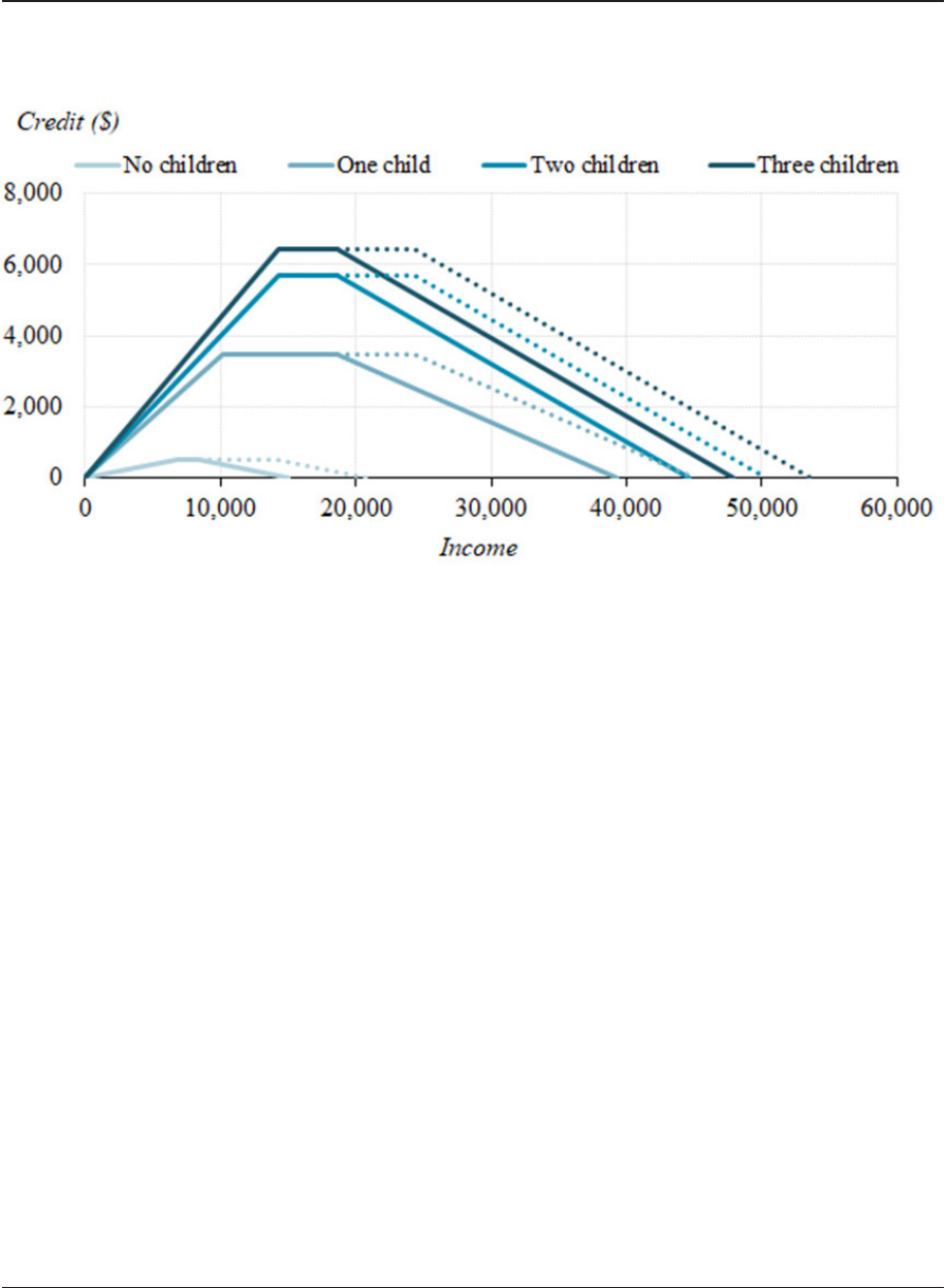
Maag, Airi, and Hunter
FIGURE 1. Earned Income Tax Credit, 2018
Source: Urban-Brookings Tax Policy Center calculations.
Notes: Assumes all income comes from earnings. Assumes children meets all tests to be EITC-qualifying children. Dotted lines represent married couples. All credit amounts are
indexed annually for ination.
e group of people who benet from the EITC is not stagnant. Prior analysis using tax data showed that
over a -year period, percent of claimants claimed the EITC for one or two years and about percent
of EITC recipients claimed the credit for more than ve years (Dowd and Horowitz ()). Credit eligibility
relies on both the income of the taxpayers and the composition of the tax unit. A tax ler needs to know who
will live in their household, their marital status, and taxpayers’ income to anticipate their EITC.
Understanding who should claim a child for the EITC creates confusion. e Treasury Department has
estimated that percent of all improper payments of the EITC stem from the incorrect person claiming the
child for credit purposes (Department of the Treasury (); Holtzblatt and McCubbin ()). e IRS indi-
cates that another two of the ve most common errors with respect to claiming the EITC are claiming a child
that does not qualify for the benet and more than one person claiming the child (IRS ()). Determining
whether an advance credit should be based on the presence of a child will presumably also be dicult for
families.
B. Child Tax Credit
e CTC osets part of the cost of raising children for working families. Expanded as part of the Tax Cuts and
Jobs Act of (TCJA), the CTC provides a benet of up to , per child under age (Figure ). Aer
rst being used to oset taxes owed, part of the CTC can be received as a tax refund. e refundable portion of
the credit is calculated as percent of earnings over ,. Prior to ,
the refundable portion of the credit
was limited to , per child. How much of the credit can be received as a refund is the only CTC parameter
indexed for ination. In , the refundable portion rose to ,. Over percent of families with children
benet from the CTC.
4
In 2021, the American Rescue Plan Act created a temporary expansion of the CTC, making the credit fully refundable. It also increased the size of the credit to up
to $3,600 per child up to age 5 and up to $3,000 per child ages 6 to 17. For more information see https://taxpolicycenter.org/brieng-book/what-child-tax-credit.
5
“Tax Benet of the Child Tax Credit (CTC) Current Law, by Expanded Cash Income Percentile, 2022,” table T21-0225, Tax Policy Center Microsimulation Model
(version 0721-1), September 2021, https://www.taxpolicycenter.org/model-estimates/tax-benets-child-tax-credit-september-2021/t21-0225-tax-benet-child-
tax-credit.

e Impact of Annual Changes in Family Structure and Income on Tax Credits
FIGURE 2. Child Tax Credit, Single Parent with One Child, 2018
Source: Urban-Brookings Tax Policy Center calculations.
Notes: Assumes all income comes from earnings. Assumes child meets all tests to be a CTC-qualifying dependent. Credit phases out beginning at $400,000 of income for married
parents. Only children with Social Security numbers qualify for the CTC. Noncitizens under age 18 who meet the dependency tests for eligibility can qualify for the other dependent
tax credit.
In addition to the refundable and nonrefundable portions of the CTC, there is also a credit for other de-
pendents (ODTC). is credit is worth up to and can only be used to oset taxes owed. Generally, the
credit is available to families with dependents who do not qualify for the CTC. Dependents of any age can
qualify for the ODTC this includes children aged or , full-time college students up to age , and children
who do not have Social Security numbers.
Claiming the CTC is less studied than the EITC. Divorced and never married parents may alternate years
of claiming a child, regardless of where the child lives the majority of the year. Because the rules for claiming
a child are less strict for the CTC than the EITC, there are likely fewer errors in who claims the credit. For
example, a child does not have to live with the claiming parent for a given number of months for the parent to
claim the child—but only one parent (or other relative) may claim the child each year.
IV. Why Do EITC and CTC Amounts Change From One Year to the Next?
A. EITC
EITC amounts depend on three main characteristics of the tax unit: the number of eligible children, earnings
and income, and marital status.
EITC amounts increase annually with ination, so even with no other chang-
es, many families will see their EITC increase from one year to the next. In the years of our study, these changes
were modest, causing the maximum credit for a family with one child to grow —from , to ,.
If the number of qualifying children in a tax unit changes, a family’s EITC will also likely change. e
number of eligible children can increase from birth, adoption, or other arrival of a new child. e number of
eligible children can decrease if a child moves to another home for more than half the year, turns during the
year, becomes the qualifying child of another tax unit in a household with cohabiting parents or multiple gen-
erations, or dies. Credit amounts increase for each additional child up to three. Increases beyond three have no
6
To a lesser extent, EITC amounts depend on investment income (which in 2018 could not exceed $3,500) and a variety of other qualifying characteristics. For
example, married couples must le a joint return; the taxpayer and spouse (if applicable) must have SSNs valid for work as do any qualifying children; taxpayers
cannot claim a foreign earned income exclusion or be the qualifying child of another person. Taxpayers without qualifying children have additional restrictions.
Internal Revenue Service, 2019. IRS Publication 596, Earned Income Credit (EIC) For use in preparing 2018 Returns. Washington, DC. Department of the
Treasur y.

Maag, Airi, and Hunter
eect and decreases above three have no eect. In many cases, a family will be able to predict these changes are
coming the next tax year, but not in all cases. Families will not necessarily know how changes in the number of
children will aect their benet. In general, a change in the number of children is the most dramatic eect. In
, increasing from no children to one child increases the maximum credit from to ,. Increasing
from two to three children increases the benet by a max of . ere are no further adjustments for children
beyond the third.
Earnings change from one year to the next for a variety of reasons. ese include changes in wage rates,
changes in the number of hours worked, changes in bonus income, changes in jobs, irregular schedules, mov-
ing in and out of the labor market. Prior research shows that among low-income families, those with income
below twice poverty, almost two-thirds have income that for at least one month of the year will spike above or
dip below their average monthly income by at least percent (Maag et al. ()). Earnings can also change
when marital status changes because the tax unit will now include income from both partners in the couple for
a newly married couple or only one partner from the couple in the case of a divorce. How the EITC changes
with income depends on whether a family has income in the phase-in period of the credit, the range where the
credit delivers a at benet, or in the phase-out range of the credit (Williams and Maag ()).
Marital status changes when people marry, divorce, or become widowed. In the case of the EITC, married
couples can earn more income before the credit begins to phase out than single people, so changing marital
status can change credit amounts—even if income amounts do not change. In particular, a couple may be able
to receive the maximum credit rather than have it partially phase down with their additional income or may
be able to receive a higher credit amount if they are in the phase-out range of the credit than when they were
single.
B. CTC
CTC amounts depend on the number of children in the family and to a lesser extent, earnings and income
amounts. e maximum benet does not change annually with ination, but instead is set at , per child
under age until , at which point it will drop to ,.
ere is no maximum number of children that can benet. e reasons for child changes in the CTC can
be the same as for the EITC, but unlike the EITC, only specic changes inform a change in the number of chil-
dren claimed for the CTC. In the case of the CTC, unmarried parents can designate who will claim the credit.
It is not necessary that the child pass the same residency test required by the EITC. In some cases, for example,
parents who do not live together have made an agreement to shi who claims the child annually. is change is
predictable for those parents. In other cases, decisions on who will claim the CTC may be made on an annual
basis and would not be any easier to predict than child residency.
e CTC phases out at relatively high-income levels (, for single parents, , for married
couples). Low- and moderate-income families may see their credit increase if earnings increase—or they may
see their credit decrease if earnings decrease. Unlike the EITC, they are unlikely to experience a credit decrease
when earnings increase because of the relatively high point at which the CTC begins phasing out. In ,
about percent of children received no credit because their parents did not earn enough. Only increases in
earnings can change their credit. About percent had earnings too low to be eligible for the full credit—an
earnings increase could increase their credit and a decrease could decrease their credit. Over percent of
children received the full credit and the vast majority would be unaected by modest changes in earnings.
e credit begins to phase out at double the income level for married couples as single parents. Changes
in marital status may aect the credit amount but are unlikely to be a large factor—except to the extent that
parents with low income marry low or moderate earners, increasing their tax unit’s total income.
7
“Distribution of Tax Units and Qualifying Children by Amount of Child Tax Credit (CTC), 2018,” table T17-0228, Tax Policy Center, October 18, 2017, https://
www.taxpolicycenter.org/model-estimates/distribution-amount-child-tax-credit-october-2017/t17-0228-distribution-tax-units.

e Impact of Annual Changes in Family Structure and Income on Tax Credits
V. Data and Methods
We use the Annual Social and Economic Supplement of the Current Population Survey (CPS ASEC) to esti-
mate year-over-year eligibility for tax credit. e CPS ASEC collects data on a representative sample of house-
holds throughout the year on a monthly basis. Households are in the survey for four consecutive months, are
out of the survey for the next eight months, and then return to the survey for another four months before leav-
ing the sample permanently. e design means that some households will be in the survey for two consecu-
tive years in March, the month that income data are collected, which can be used to estimate taxes including
refundable tax credits. We use this feature of the survey to follow households with at least one child under age
who appear in the survey in two consecutive years. We use the Transfer Income Model, version (TRIM),
to estimate changes in the EITC and CTC from one year to the next.
We exclude from our sample households
where income was imputed because imputations are not designed to show changes from one year to the next.
Our analysis uses data from through , which represent income amounts from through .
We pair observations in and , and , and and . We apply tax law in all years: our
calculations were therefore unaected by the Tax Cuts and Jobs Act’s changes to the CTC that went into eect
in . A household must have a child in at least one year to be part of our sample.
VI. Results
We compare the EITC and CTC that a tax unit appears eligible for in year two with the credit they appear
eligible for in year one.
All of the families in our analysis have a child in either the rst or second year they
are observed. For each credit, we group tax units into those with an increase in the credit of at least from
year one to year two, those that have a change of less than , and those with a credit decrease of at least
between the two years. Low-income families are dened as those with incomes beneath percent of
the ocial poverty measure.
A. Earned Income Tax Credit
Not all families are eligible for an EITC in both years. In our data, about percent of families with children
receive an EITC in at least one year and percent receive no EITC in both years. We estimate that percent
of families experience a drop in their EITC of at least , over two-thirds of families ( percent) have no
major change in eligibility, and the remaining percent of families appear eligible for an EITC that is at least
larger in year two than in year one (Figure ).
Among low-income families with children, those with income below twice the poverty level in year one,
we observe that percent receive an EITC in at least one year and percent receive no EITC in both years.
We estimate that percent of families experience a drop in their EITC of at least , some percent have
no major change in eligibility, and the remaining percent see their credits increase by at least .
Income changes drive earned income tax credit changes and large earned income tax credit changes are
most common
If a family’s income is in the phase-in range of the credit, a decrease in income results in a year-over-year
decrease in the EITC. A suciently large decrease in income from the plateau range of the credit can also
8
Information presented here is derived in part from the Transfer Income Model, version 3 (TRIM3), and associated databases. TRIM3 requires users to input
assumptions and/or interpretations about economic behavior and the rules governing federal programs. erefore, the conclusions presented here are attributable
only to the authors of this report.
9
Our data do not allow us to implement the rules that all persons in the tax unit must have a Social Security number (SSN) eligible for work to be eligible for the
EITC. Although TRIM3 models SSN requirements, the TRIM3 imputation of whether a person has an SSN is not necessarily consistent in two consecutive years
of CPS data and so we do not use those imputations for this analysis. We allow the EITC parameters to adjust with ination but deliver a maximum CTC benet
of $2,000 per child with up to $1,400 allowed as a refund, consistent with 2018 law.
10
Because the CPS is a household survey, we cannot track people who move households. We can track changes that happen to a tax unit if the tax unit stays in the
same household. For example, if a couple divorces, and one partner remains in the household, we can compare the EITC and CTC the partner who stayed in the
household qualied for in year two with the EITC and CTC the partner was eligible for as part of a couple in year one. In this way, our estimates likely overstate
stability in the tax credits because people moving homes are probably more likely to experience a change in credits than people remaining in the same home.

Maag, Airi, and Hunter
decrease the credit. Income increases can also have the opposite eect. An increase in income can decrease
benets if a person’s income moves into or farther into phase-out range of the credit.
An increase in income can happen because a person works or earns more—but also when couples marry,
and additional income may become available to the tax unit. We nd that over percent of the low-income
families that experience a decrease in their EITC experience that decrease because of an increase in earnings
(representing percent of all low-income families in our sample).
e remaining families that see an EITC
drop of at least from one year to the next are split roughly evenly between families where the number of
children decreased and families where income decreased and caused the EITC to decrease. Changes in other
household characteristics such as marital status not accompanied by changes in income or children aect un-
der percent of low-income families.
In some cases, drops in the EITC from one year to the next can be dramatic. Among low-income families,
about percent see a drop of at least , and another percent see a drop of between , and ,
(Figure ). Drops of at least , are caused by income increasing percent of the time, children decreasing
percent of the time, and income decreasing percent of the time.
FIGURE 3. Year-to-Year Changes in Earned Income Tax Credit Amounts for Families with
Children, 2018 Tax Law
Source: Urban Institute TRIM3 model using data from Current Population Survey Outgoing Rotation Groups 2015–18.
Notes: Sample includes households with one dependent child under age 18 in either year. No change is dened as a change of less than $500.
About percent of low-income families with children become eligible for a larger EITC in the second
year than in the rst. Changes in income drive increases in the EITC for these low-income families about
percent of the time ( percent of low-income families see their EITC increase because their income decreased,
and another percent of low-income families see their EITC increase because their income increased). For
percent of low-income families, we observe an EITC increase driven by the number of children in the tax unit
11
Decrease in earnings is dened as a decrease in earnings without a change in the number of children over the same period.

e Impact of Annual Changes in Family Structure and Income on Tax Credits
increasing. About half of all low-income families with an EITC increase see an increase of more than ,.
A small share of low-income families become newly eligible for an EITC in the second year we observe them
aer having no earnings in the rst year.
Demographic variations in earned income tax credit changes among low-income households
We estimate whether the likelihood of an EITC increase or decrease varies by demographic characteristics
for those with income below percent of the federal poverty level in year one (Figure ). About percent
of white non-Hispanic and percent of Black non-Hispanic households receive no credit in both years, or
have no major change in their credit amount from year one to year two. Hispanic families were less likely to
experience no change in eligibility, about percent. While the share of families, by race and ethnicity, that
experienced an increase in the amount of EITC they were eligible for from year one to year two was roughly
the same, Hispanic families were more likely to see their EITC drop than white, non-Hispanic or Black, non-
Hispanic families.
FIGURE 4. Year-to-Year Changes in Earned Income Tax Credit Amounts,
2018 Tax Law
Source: Urban Institute TRIM3 model using data from Current Population Survey Outgoing Rotation Groups 2015–18.
Notes: Sample includes households with one dependent child under age 18 in either year with incomes below twice federal poverty level in the rst year observed.
No change is dened as a change of less than $500. Marital status is shown only for those with same marital status in both years. Families with marital status
changes excluded due to small sample size.
People who were low-income and unmarried in both years of our sample were more likely to maintain
similar EITC eligibility in year two ( percent) than people who were married ( percent). is may be
because with only one potential earner in the tax unit, there is less opportunity for variation. In a married

Maag, Airi, and Hunter
couple, two people may be exposed to changes in employment. About percent of unmarried adults with low
incomes in our sample saw the amount of credit they were eligible for decline by at least in year two and
the remaining percent saw their credit amount increase.
Younger adults with low incomes were more likely to see their EITC change from year one to year two
than households where the survey respondent was either under or over age . While just percent of
adults under age and percent of adults ages to experienced no change in credit eligibility, over half
of adults in our older group had no major change in credit eligibility. In many cases, it was because older tax
lers were more likely to be ineligible for a credit in both years. Most changes in predicted eligibility were
greater than .
B. Child Tax Credit
Over percent of all families with children received a CTC in either year, compared with percent of
families with incomes under percent of the federal poverty level. Among families with low incomes that
received no CTC, some had no earnings or earnings below , and others had children aged out of eligibil-
ity for the program. Children must be under age to qualify for the CTC. Older limits apply for children to
qualify for the EITC. Just over percent of all families with children saw no major change in CTC eligibility
for from year to year (a change of less than ). Forty-nine percent of low-income families with children
saw changes of less than from one year to the next. Among those that saw their credits change by at least
, roughly half saw their credits increase and the other half experienced a credit decrease. Among families
with low-incomes, more saw an increase in their CTC from one year to the next than saw a credit decrease.
Year-over-year CTC Decrease
Just over percent of all families with children and percent of low-income families with children experi-
enced a drop in credit eligibility of at least from year one to year two. A drop in the number of children
in the tax unit was associated with percent of CTC decreases over . Among those percent, about
half of families with CTC decreases of at least had a child age out of CTC eligibility. Among low-income
families, income drops and reductions in the number of children contributed similarly to declines in credit
eligibility.
Year-over-year CTC Increase
Among families with children, percent of all families became eligible for a credit of at least higher in
the second year and percent of low-income families saw the same. Just under half of credit increases were
driven by an increase in the number of qualifying children, and nearly a quarter by an increase in children
because of the birth or adoption of a child between years one and two. Among low-income families, credit
increases most oen stemmed from an increase in income. is allowed families to either move further up
the phase-in of the credit or have additional tax liability that could be oset with the nonrefundable portion
of the CTC. Among low-income families, a smaller share of CTC increases was attributable to increases in the
number of children. For families with incomes too low to qualify for any CTC, an increase in children has no
eect on their credit.
Most families whose credit decreased did so by amounts between , and ,. About percent of all
families and percent of families with incomes below percent of the federal poverty level in year one fell
by this amount (Figure ). For families experiencing a credit increase, the majority ( percent of all families)
had an increase of at least ,. is likely indicates a new child joining the tax unit.

e Impact of Annual Changes in Family Structure and Income on Tax Credits
FIGURE 5. Year-to-Year Changes in Child Tax Credit Amounts for Families With
Children, 2018 Tax Law
Source: Urban Institute TRIM3 model using data from Current Population Survey Outgoing Rotation Groups 2015–18.
Notes: Sample includes households with one dependent child under age 18 in either year. No change is dened as a change of less than $500.
Comparing changes in credit by race and marital status among families with children with income below
percent of the federal poverty level, we see few dierences. In general, families with income below
percent of the federal poverty level are more likely to see their credit increase ( percent) than decrease (
percent). We observe greater volatility in credit amounts among families where the parent that responded to
the survey was between ages and (Figure ).
FIGURE 6. Year-to-Year Changes in Child Tax Credit Amounts, 2018 Tax Law
Source: Urban Institute TRIM3 model using data from Current Population Survey Outgoing Rotation Groups 2015–18.
Notes: Sample includes households with one dependent child under age 18 in either year with incomes below twice federal poverty level in the rst year
observed. No change is dened as a change of less than $500. Marital status is shown only for those with same marital status in both years. Families with
marital status changes excluded due to small sample size.

Maag, Airi, and Hunter
VII. Discussion
Refundable tax credits like the EITC and CTC provide substantial support to families with children. Low- and
moderate-income families oen receive the credits as a single payment at tax time—but there is interest in
delivering credit through the year, building on the experience of a temporary expansion of the CTC in .
But advancing credits is not without risk if families must pay them back if they end up receiving them errantly.
Our analysis estimates the size of year-over-year changes in the EITC and CTC to understand better
how feasible it might be to deliver a tax credit based on information from the prior year’s tax return. Credits
delivered in advance must be based on some information. If families or the IRS were to use information from
a current tax return to predict their next year’s credit, our analysis shows how oen they are likely to make a
prediction within . Because credits are based on income, qualifying children (and in the case of the EITC
where they reside most of the year), and marital status, families (or the IRS) would need to guess at some fac-
tors. No administrative data exist with this information, though prior research has retrospectively examined
patterns of EITC participation by constructing panel datasets with tax return administrative data (Ackerman
et al. (); Dowd and Horowitz ()). In prior work, we explored using administrative data to determine
eligibility for credits and it was largely insucient (Pergamit et al. ()). ere are also shortcomings in the
survey data used in this analysis: unstable households that move addresses are least likely to remain in the
CPS sample. Consequently, our results could understate volatility in household arrangements, income, and
tax credits.
We are more concerned with credit changes for low-income families who likely would have more diculty
paying back errantly delivered tax credits than high-income families. Moreover, they are likely to be harmed
more by not getting advance credits, and recent evidence following the monthly delivery of the CTC from July
to December suggests lower-income households are more interested in advance monthly payments than
others (Maag and Karpman ()).
Among low-income families with children, those with incomes below percent of the federal poverty
level, percent received no EITC in either the rst or second year we observed them in national data, and
percent saw their EITC change by less than from one year to the next. Advance credits could be designed
to not deliver the entire benet in advance or limit the amount of errantly delivered credit that would need to
be repaid—though this would cost the government revenue. We nd that percent of low-income families
see their EITC drop by at least and percent see their EITC increase by at least from one year to
the next. About percent of low-income families saw their EITC drop from one year to the next because their
income increased (about percent of all families that saw an EITC drop).
Among low-income families with children, we estimate percent receive no CTC in either year—oen
because they have no earnings or their children are over age , the oldest qualifying age for the credit. Another
percent see their CTC change by less than . About percent of low-income families see their CTC
drop by at least and the remaining percent see their CTC increase by at least . e largest groups
that see credit changes are related to an increase in earnings. In the case of the CTC, percent of low-income
families saw their CTC increase because their earnings increased (about two-thirds of the low-income families
that saw their CTC increase from one year to the next).
Families also see credits change because the number of children in the tax unit change or their marital
status changes. ese changes are less common than income changes but still aect a signicant group of
people. We estimate that percent of all low-income families experienced a CTC increase because the num-
ber of children in the tax unit increased and almost percent saw their CTC decrease because the number of
children in the tax unit decreased. About percent of EITC changed because the number of children in the
household changed—divided evenly by EITC increases and decreases. Families that change from one year to
the next (through marriage, divorce, or change in the number of children) are likely to see credit changes of
at least ,.
Tax credits increasing and decreasing year over year introduces a source of income volatility among low-
income families that in some cases can be positive—family income jumps more than expected because tax

e Impact of Annual Changes in Family Structure and Income on Tax Credits
credits are higher than expected. In other cases, it can present a negative shock as tax credits drop. Analysis
shows that these changes are oen a surprise to families (T. Anderson et al. ()).
A. Implications of Volatility
Not all income volatility is experienced in the same way by families—and some is more predictable than oth-
ers. When income increases, which oen happens at tax time when tax refunds are delivered, families have
new opportunities present. Families might invest in items such as a used car or childcare that can help with
increasing employment or might invest in a relatively large purchase like a refrigerator. Evidence also suggests
that families are more likely to go to the doctor following receipt of a tax refund (Hamad and Niedzwiecki
()) and families with older children are more likely to enroll in school (Manoli and Turner ()). If ad-
vance credits are delivered throughout the year, presumably refunds would be smaller—but it also might be
the case that refunds could disappear altogether or families could unexpectedly owe taxes if too much credit
is delivered in advance.
When changes in tax credits are foreseeable because children are aging out of eligibility, the IRS, tax
preparers, and community organizations can work to educate taxpayers about coming changes. Trusted mes-
sengers, or third parties regarded as credible by families that face barriers to navigating the tax system, can
increase tax benet participation and are well-situated to relay tax information throughout the year (Cox et
al. (); Airi et al. (); Godinez-Puig et al. ()). In some cases, families will know they are likely to
add another child either through birth or adoption. Other times, changes can be more dicult to predict, and
it’s unlikely that families could be warned appropriately. It may be the case that custody of a child changes
abruptly and who lives together can also change. e IRS would know about these changes only if families or
third-party assistants were able to apprise the IRS of the changes, in which case advance credits that were be-
ing delivered could be stopped or started, as appropriate. In the recent experience with the IRS portal for the
expanded CTC, few families updated information through the portal (GAO ()).
Decreases in the credits are more concerning because that could put families in the vulnerable position
of needing to repay the IRS. In many cases, income swings that appear to be driving a lot of the year-over-
year changes we observe would not be predictable, absent new reporting requirements. And, as with family
changes, only if the IRS were notied quickly could advance payments be stopped to limit a family’s potential
liability.
VIII. Conclusion
Refundable tax credits provide an important source of income for families with low incomes. Determining
who can claim a child can be complicated by family structure and living arrangements. As the share of mar-
ried couples with only biological children declines and the share of children in shared custody arrangements
rises, ling a tax return can become more complex. Families must determine what tax unit a child should be
properly assigned to—and how that decision is made can have a dramatic impact on who will benet from
the EITC and CTC. Importantly, the determination is made on an annual basis and only one family can get a
tax benet for a given child—even when multiple families share custody of a child. Changes in the number of
children that a family can claim, income, and marital status (which can itself aect income) can all drive large
credit changes from one year to the next.
Most families experience year-over-year changes in their EITC or CTC of less than . When cal-
culating the EITC, this oen happens because families are eligible for no credit in either year one or year
two. Among low-income families, those with income below twice the federal poverty level, percent have a
change of less than in their EITC, and about half have a change of less than in their CTC. A virtually
identical share of families with no change in marital status or number of children have a change of less than
in their EITC and percent of these families have a change of less than in their CTC.
Among low-income families with children, about percent see their EITC decrease by more than
and percent see their CTC decrease by more than . Most oen, when families experience a drop in their
EITC, it is because their earnings increase. In some cases, this is because a single parent marries, bringing a

Maag, Airi, and Hunter
new source of income into the tax unit. Conversely, a decrease in earnings is the most common reason for
an increase in the EITC (families are moving from beyond the phase-out or in the phase-out range to the
maximum credit range), which shows how the credit can mitigate a loss in income in some cases. When a low-
income family’s CTC increases, it oen does so because of an increase in income rather than a change in the
number of children in the tax unit. is is because low-income families have their credit limited by their earn-
ings not being enough to access more credit—but very few will see earnings increase large enough to result in
the credit beginning to phase out.
Helping families understand how credits are calculated might help them predict when a credit will in-
crease or decrease. is is important because it could help families understand the nancial position that they
will be in at tax time the following year. Understanding how credits change from year to year can also help
policy makers design advance credits that can be delivered without putting families at risk. For example, policy
makers can design provisions that protect a certain amount of credit from being clawed back at tax time if too
much credit has been delivered in advance.
Our research suggests that protecting about of each advance credit would protect most families from
needing to repay credits at tax time. ese protections would cover a smaller share of low-income families,
especially with respect to the EITC, which suggests that further measures are needed to protect low-income
families in particular. Otherwise, an advance credit based on last year’s tax return could result in a disruptive
tax bill. While steps might be available to mediate changes in credit stemming from changes in income (de-
pending on how soon they were reported), family changes present additional challenges.

e Impact of Annual Changes in Family Structure and Income on Tax Credits
References
Ackerman, Deena, Janet Holtzblatt, and Karen Masken. 2009. “e Pattern of EITC Claims Over Time: A
Panel Data Analysis.” Recent Research on Tax Administration and Compliance: Selected Papers Given at the
2009 IRS Research Conference, IRS Research Bulletin. Washington, DC: Internal Revenue Service.
Airi, Nikhita, Luisa Godinez-Puig, and Kim Rueben. 2022. “Helping New Mothers Understand the Benets of
Filing Taxes.” Washington, DC: Tax Policy Center.
Anderson, Lydia, Paul F. Hemez, and Rose M. Kreider. 2022. “Living Arrangements of Children: 2019.”
Suitland, Suitland-Silver Hill, MD: US Census Bureau.
Anderson, eresa, Amelia Coey, Hannah Daly, Heather Hahn, Elaine Maag, and Kevin Werner. 2022.
Balancing at the Edge of the Cli: Experiences and Calculations of Benet Clis, Plateaus, and Trade-Os.
Washington, DC: Urban Institute.
Caldwell, Sydnee, Scott Nelson, and Daniel Waldinger. 2023. “Tax Refund Uncertainty: Evidence and Welfare
Implications.” American Economic Journal: Applied Economics 15 (2): 352–76.
CBO (Congressional Budget Oce). 2019. “Marginal Federal Tax Rates on Labor Income: 1962 to 2028.”
Washington, DC: CBO. https://www.cbo.gov/system/les/2019-01/54911-MTRchartbook.pdf.
Cox, Kris, Roxy Caines, Arloc Sherman, and Dottie Rosenbaum. 2021. “State and Local Child Tax Credit
Outreach Needed to Help Li Hardest-to-Reach Children Out of Poverty.” Washington, DC: Center on
Budget and Policy Priorities.
Dowd, Tim, and John B. Horowitz. 2011. “Income Mobility and the Earned Income Tax Credit: Short-
Term Safety Net or Long-Term Income Support.” Public Finance Review 39 (5): 619–52. https://doi.
org/10.1177/1091142111401008.
Department of the Treasury. 2018. “Financial Report of the United States Government: Fiscal Year 2017.”
Washington, DC: Department of the Treasury.
Fox, Liana, and Kalee Burns. 2020. “e Supplemental Poverty Measure: 2019.” Suitland, Suitland-Silver Hill,
MD: U.S. Census Bureau.
GAO. 2022. “Current and Future Federal Preparedness Requires Fixes to Improve Health Data and Address
Improper Payments.” Washington, DC: Government Accountability Oce.
Godinez-Puig, Luisa, Aravind Boddupalli, and Livia Mucciolo. 2022. “Lessons Learned from Expanded Child
Tax Credit Outreach to Immigrant Communities in Boston.” Washington, DC: Tax Policy Center.
Hamad, Rita, and Matthew J. Niedzwiecki. 2019. “e Short-Term Eects of the Earned Income Tax Credit
on Health Care Expenditures among US Adults.” Health Services Research 54 (6): 1295–1304. https://doi.
org/10.1111/1475-6773.13204.
Holtzblatt, Janet and Janet McCubbin. 2002. “Issues Aecting Low-Income Filers.” In e Crisis in Tax
Administration edited by Henry Aaron and Joel Slemrod, 148–200. Washington, DC: Brookings Institution
Press.
IRS (Internal Revenue Service). 2022. “Common Errors for the Earned Income Tax Credit (EITC).” Washington,
DC: IRS.
IRS (Internal Revenue Service). 2022. “Handling the Most Common Errors.” Washington, DC: IRS.
Maag, Elaine, H. Elizabeth Peters, Sara Edelstein. 2016. Increasing Family Complexity and Volatility: e
Diculty in Determining Child Tax Benets. Washington, DC: Urban Institute.
Maag, Elaine, H. Elizabeth Peters, Anthony Hannagan, Cary Lou, Julie Siwicki. 2017. Income Volatility: New
Research Results with Implications for Income Tax Filing and Liabilities. Washington, DC: Urban Institute.
Maag, Elaine, and Michael Karpman. 2022. “Many Adults with Lower Income Prefer Monthly Child Tax
Credit Payments.” Washington, DC: Urban Institute.

Maag, Airi, and Hunter
Manoli, Day, and Nicholas Turner. 2018. “Cash-on-Hand and College Enrollment: Evidence from Population
Tax Data and the Earned Income Tax Credit.” American Economic Journal: Economic Policy 10 (2): 242–271.
https://doi.org/10.1257/pol.20160298.
Meyer, Daniel R., Maria Cancian, and Steven T. Cook. 2017. “e Growth in Shared Custody in the United
States: Patterns and Implications.” Family Court Review 55: 500–12. https://doi.org/10.1111/fcre.12300.
Michelmore, Katherine M., and Natasha V. Pilkauskas. 2022. “e Earned Income Tax Credit, Family
Complexity, and Children’s Living Arrangements.” e Russell Sage Foundation Journal of the Social Sciences
8 (5): 143–65. https://doi.og/10.7758/RSF.2022.8.5.07.
Morduch, Johnathan, and Rachel Schneider. 2017. e Financial Diaries: How American Families Cope in a
World of Uncertainty. Princeton: Princeton University Press.
National Taxpayer Advocate. 2020. “Earned Income Tax Credit: Making the EITC Work for Taxpayers and
Government.” Washington, DC: National Taxpayer Advocate.
Pergamit, Michael R., Elaine Maag, Devlin Hanson, Caroline Ratclie, Sara Edelstein, and Sarah Minton.
2014. 2014 Pilot Project to Assess Validation of EITC Eligibility with State Data: Final Report. Washington,
DC. Urban Institute.
Romich, Jennifer L., and omas Weisner. 2000. “How Families View and Use the EITC: Advanced Payment
versus Lump-sum Delivery.” National Tax Journal 4 (2). https://doi.org/10.17310/ntj.2000.4S1.09.
Williams, Roberton, and Elaine Maag. 2008. “e Recession and the Earned Income Tax Credit.” Washington,
DC: Urban Institute.

2
∇
Estimating Audit Aershocks
Besnek Partington
Lindsay Grana McGlothlin Plumley
Plumley Rodriguez Grana McGlothlin

Changes to Voluntary Compliance Following
the Random Enquiry Program on Income
Tax Returns
Murat Besnek and Allan Partington (Australian Taxation Oce)
1. Introduction
ere are three ways audits impact revenue collected by tax administrators. First, through adjustments, penal-
ties, and interest payments made during the audit process when correcting the taxpayer’s initial misreported
liability (audit yield). Second, through changes to future voluntary compliance of audited taxpayers where the
audit inuences the subsequent reported liabilities (direct deterrent eect). ird, through spillover eects on
non-audited taxpayers whose reported liabilities are inuenced in part by their expected probability of an au-
dit, based on their observation of the tax administration’s activities (indirect deterrent eect). Tax administra-
tors have precise information about audit yields; however, less is known about the direct and indirect deter-
rent eects. Moreover, even though there is extensive literature on tax evasion,
1
the literature on behavioural
changes of taxpayers is limited (Advani et al. (2019); Beer et al. (2015); Gemmell and Ratto (2012)).
Activities like audits are commonly used by tax administrators to increase tax compliance. Without these
strategies, taxpayer contributions would be expected to be limited in the absence of strong altruistic motiva-
tions. We know—as do rational taxpayers—that it is not nancially possible to pursue every taxpayer who is
noncompliant because of audit costs. So, the payo for noncompliance is an expected value—the payo mul-
tiplied by the probability of not being caught. e more credible the threat of an audit, the lower the payo for
noncompliance, making it more benecial to comply with the tax system (Bergolo et al. ()).
In this paper, we estimate the direct deterrent eect of Random Enquiry Program (REP) audits on tax
returns, performed by the Australian Taxation Oce (ATO) in , , and . e audits include tax-
payers from the individuals not in business (INIB); small business–individuals in business (SB-IIB); and small
business–small company (SB-SC) population types. e estimate can be used to determine the intertemporal
benets (costs) of audits, potentially inuencing the number of audits being allocated to certain populations
and/or to audits in general. Estimates of the indirect deterrent eect are beyond the scope of this study.
One recommendation we adopt from Gemmell and Ratto () is to separately test the responses of the
so called “compliant” and “noncompliant” taxpayers.
is enables us to see the heterogenous treatment ef-
fects without allowing them to cancel each other out. As a point of dierence during the estimation phase, we
use the Poisson Pseudo Maximum Likelihood (PPML) estimator rather than ordinary least squares (OLS).
We believe that the PPML estimator has two distinct advantages: () it removes the need to alter zero-inated
datasets
and () the results do not rely on the normal distribution assumption (Bellego et al. ()).
While we nd that the audits change voluntary compliance, the results depend on the population type
of the taxpayer, and if the audit nds them to be compliant or noncompliant. For instance, we nd that the
noncompliant taxpayers in the INIB population have a negative direct deterrent eect.
In contrast, we nd
that the noncompliant taxpayers in the SB-IIB and SB-SC populations have a positive direct deterrent eect.
1
For instance, the tax gap estimates provided by the Australian Taxation Oce.
2
Being noncompliant hinges upon an error being detected during the audit process.
3
For example, in Gemmell and Ratto (2012), all the observations where y
i
= 0 is removed.
4
at is to say that they report lower liabilities in the post-audit years than the control group.

Besnek and Partington
Seventy-eight percent of taxpayers in the INIB population are noncompliant, so obtaining statistically sig-
nicant estimates for the compliant taxpayers in this population are not possible. e compliant taxpayers in
the SB-IIB (SB-SC) population have a positive (negative) direct deterrent eect. e largest (smallest) overall
audit yield is found in the SB-IIB (INIB) population. e audit treatment eects appear to remain steady for
all population types. ere is no indication of returning to the levels displayed by their control groups over the
multiple years following the audit allocation date,
which were covered by the study.
Our future research will involve extending the analysis by using audits on income tax returns from
the REP. In addition, possibly incorporating the risk-based audits from the operational data to see if the risk-
based audits produce dierent results. Estimating the indirect deterrent eect may also happen at some point
in the future. e remainder of the paper is organised as follows: Section 2 describes the data and discusses
who is considered noncompliant; Section 3 explains the empirical methodology; Section 4 presents the results
by considering what the estimated intertemporal benets (costs) of audits imply to the current compliance
activities undertaken by the ATO; and Section 5 concludes the paper.
2. Data
e REP involves auditing the returns of randomly selected taxpayers from the INIB, SB-IIB and SB-SC popu-
lations. For this study, there are three REP datasets available,
6
separated by the nancial year of the taxpayers’
net tax amount
7
under investigation. Each dataset is analysed individually, but we also provide a pooled esti-
mate. e data only includes taxpayers that are contacted by the ATO, using allocation date as a proxy for the
date the taxpayers are contacted. Due to internal proling, some taxpayers are not contacted by the ATO, and
as a result, are not included in this study (see below for more details about internal proling).
For each dataset, using the same sampling approach, we randomly select a control group that is approxi-
mately ten times larger than the treated. We check that the control groups do not include any taxpayers that
are contacted by the ATO for other reasons during the period of the study. A Wilcoxon rank-sum test is then
applied to conrm that the net tax amounts of the treated and control groups are similar in the pre-audited
periods. If the Wilcoxon rank-sum test fails, a new control group is selected until the test passes. so that the
treated and control groups are comparable. Once the taxpayers are comparable, we acquire the net tax amount
for each taxpayer between the nancial years of 2011–2020. We ensure that our analysis only focuses on vol-
untary compliance. For instance, we remove the 2015 net tax amount for taxpayers that are a part of the 2015
sample. is applies to taxpayers in the treated and control groups.
e INIB population consists of taxpayers with no business connection. ey are typically individual enti-
ties other than those identied as being in or linked to small business, high wealth or wealthy Australians or
recipients of passive or personal services income (PSI). e small business population focuses on small busi-
nesses, SB-IIB being individuals and SB-SC being companies. e individuals in the small business population
include taxpayers with (i) turnover less than $10 million (ii) exclusive connections to small businesses with
aggregated turnover less than $10 million, (iii) links to small business entities in the capacity of being a share-
holder, director, trustee or partner, and (iv) PSI recipients. e companies in the small business population
have an aggregated turnover less than $10 million and are not controlled by high wealth groups (being groups
with net assets greater than $50 million with an ownership level greater than 40%).
e taxpayers in the REP are subject to internal proling when they are selected. To minimise the burden
on taxpayers, where income can be matched to a third-party dataset on the ATO system and the amounts
that cannot be veried are immaterial, these returns are not investigated further. Such taxpayers are accepted
as having no (or immaterial) tax adjustments. e remainder of the taxpayers in REP are then escalated to a
review to determine material amounts that could not be veried. e review covers, but may not be limited to:
5
Allocation date refers to the date when the taxpayer is allocated to an auditor to commence the case.
6
2015, 2016 and 2017.
7
Net tax amount is tax on taxable income plus Medicare levy minus non-refundable osets.

Changes to Voluntary Compliance Following the Random Enquiry Program on Income
Tax Returns
• Compliance history of the taxpayer;
• Recent nancial performance of the business;
• Comparisons of declared income and expenditure;
• Checking merchant activity for credit card sales;
• Comparison with industry benchmarks;
• ATO risk ags; and
• Property ownership.
As well as reviewing the aairs of the taxpayers, any directly associated individuals and entities are also
reviewed. ese associates may include:
• Spouse and family members;
• Partners and partnerships;
• Companies, directors and shareholders; or
• Trusts.
Where issues are found, taxpayers are taken to the next stage, which is an audit. Only the taxpayers that
are escalated to an audit are included in this study as there is no taxpayer contact during the review stage. We
would expect the behaviour of the veried and reviewed taxpayers to be no dierent than the control group.
Approximately % of the INIB, % of SB-IIB and % of the SB-SC populations are removed from REP
samples. Leaving behind , audits for the INIB, audits for the SB-IIB, and audits for the SB-SC
populations. Figure provides a breakdown across the three nancial years.
FIGURE 1. REP Sample Size
Financial Year is the rst time the REP took place, so the sample size is a little smaller. Sample size be-
tween INIB and small business (SB-IIB+SB-SC) is comparable over time; though, one thing to note is that the
small business population contains more companies than individuals. e size of the datasets is capped due to
resources allocated to the REP, even though it would be benecial to have more treated observations for this
study. In terms of noncompliance, individuals seem to perform worse than companies. e INIB population is
approximately % noncompliant. Companies, on the other hand, seem to conform a lot better with their tax
obligations, never exceeding % in noncompliance, which can be observed from Figure .

Besnek and Partington
FIGURE 2. Noncompliance as a Percentage of REP Sample Size
As expected, the audit yields are lower for the INIB population than for small businesses. e average
audit yield for INIB is equal to , in , , in and in . If we use the pooled dataset, the
average audit yield for INIB equals ,. e average audit yield for SB-IIB is equal to , in , ,
in and , in . If we use the pooled dataset, the average audit yield for SB-IIB equals ,. e
average audit yield for SB-SC is equal to in , , in and , in . If we use the pooled
dataset, the average audit yield for SB-SC equals ,. It is also apparent from Table that the audit yields are
not enough to cover the costs of running the REP.
TABLE 1. Average Audit Yield
AVERAGE 2015 2016 2017 POOLED
INIB $1,071 $1,098 $881 $1,018
SB-IIB $3,914 $2,001 $12,253 $6,936
SB-SC $900 $2,705 $4,129 $2,433
REP AVERAGE $1,962 $1,935 $5,754 $3,462
3. Empirical Methodology
Tax administration research frequently uses positively skewed datasets where the dependent variable equals
zero on a regular basis. Under these circumstances, using OLS for statistical inference is not appropriate, due
to the violation of the normality assumption. e common solution is to use a log-transformed dependent
variable. However, logging the dependent variable is not ideal due to Jenny’s inequality. Jenny’s inequality im-
plies that E(ln(y) )≠lnE(y), so retransforming the log terms will result in a biased estimate (Motta ()). is
estimate will then need to be adjusted for heteroscedasticity.
Another major issue with logging the dependent variable is the inability to log zeros. If we decide to take
this approach, we need to add a positive constant to all the observations where the dependent variable equals
zero or delete them altogether like Gemmell and Ratto (). However, removing the zeros or giving them a
small positive value can worsen the heteroscedasticity (Motta (2019)). Moreover, the size of the positive con-
stant will depend on the data at hand, adding the smallest possible value (for example, the value of 1) is not the
least harmful choice. Bellego et al. (2021) show that the best value for the positive constant is not necessarily
small, nor equal to 1, contrary to common belief.
Using the PPML estimator is a better alternative to correcting the bias of a log-transformed dependent
variable because it can handle observations where the dependent variable equals zero (Silva and Tenreyro

Changes to Voluntary Compliance Following the Random Enquiry Program on Income
Tax Returns
(); Correia et al. ()). is estimator is popular because the only condition required for consistency is
the correct specication of the conditional mean. erefore, the data does not need to have a Poisson distribu-
tion, nor does the dependent variable need to be an integer (Gourieroux et al. ()). Although, with continu-
ous variables, the assumption that the conditional mean equals the conditional variance is unlikely to hold.
For this reason, the standard errors need to be based on the Eicker- Huber-White robust covariance estimator.
To measure the change in voluntary compliance of audited taxpayers, we use a dierence in dierences
(DID) model. We begin by subtracting the pre-audit net tax amount from the post-audit for treated taxpay-
ers.
8
We denote this dierence d . Any dierence in d can be a result of the REP, but also other possible events.
To account for this, we repeat the same process for the control group. We denote this dierence d. Subtracting
d from d produces the standard DID model and it can be estimated using the following regression:
y
it
=β
0
+β
1
D
PostAudit
+β
2
D
Treated
+β
3
D
PostAudit
×D
Treated
+ e
t
,
where y
it
is the net tax amount for taxpayer
i
in year t, D
PostAudit
, is a dummy variable for the post-audit observa-
tions D
Treated
, is a dummy variable for the treated taxpayers, and e is a random error term.
e interpretation of the coecients is as follows: β equals the average pre-audit and β+β equals the
average post-audit net tax amounts for the control group. β
+β
equals the average pre-audit and β
+β
+β
+β
equals the average post-audit net tax amounts for treated taxpayers. β is the DID parameter that quanties
the impact of the audit.
In Gemmell and Ratto (), a modied version of the DID model is specied. e purpose of the speci-
cation is to avoid combining the positive and negative impacts of audits. If we do not separately test the
responses of compliant and noncompliant taxpayers, there is a chance that we incorrectly conclude that audits
do not impact taxpayer behaviour. e REP does keep records of other personal information. However, due
to the small sample size, it is not possible to include them in the DID regression. Other than year, population
type, and taxpayer compliance, we could not control for any other taxpayer characteristics. e version of the
DID model we use in this study is specied below:
y
it
=β
0
+β
1
D
PostAudit
+β
2
D
PostAudit
×D
Compliant
+β
3
D
PostAudit
D
NonCompliant
+δ
i
+e
t
with notation as described before and where D
Compliant
is a dummy variable for the compliant taxpayers,D
NonCompliant
is a dummy variable for the noncompliant taxpayers, δ
i
are individual xed eects.
Interpretation of the coecients is as follows: β+β equals the average post-audit net tax amount for the
control group. β
+β
+ β
equals the average post-audit net tax amount for the compliant taxpayers. β
0
+β
1
+β
3
equals the average post-audit net tax amount for the noncompliant taxpayers. β (β) is the DID parameter that
quanties the impact of the audit on compliant (noncompliant) taxpayers.
One thing to note is that when the model does not separate taxpayers based on their compliance, we do
not need to control for unobservable characteristics, as random sampling ensures that there are no systematic
dierences across the groups. However, when we run the DID model where the treated taxpayers are divided
into subgroups, we need to run the PPML estimator with individual xed eects. is is to allow for the pos-
sibility that there are systematic dierences across the groups. As long as these dierences stay consistent
(xed) between the time periods of interest, the individual xed eects (δ
i
) coecient will control for these
dierences, even if they are unobservable.
4. Results
Each subsection below provides a detailed breakdown of the direct deterrent eect for a specic population
arranged by nancial year. We obtain these results using reliable audit data sourced from the ATO. We employ
the industry standard during the estimation phase, that being the PPML estimator (following the advice of
Jeery Wooldridge and many other academics). e model we use has no impact on the direction of the direct
8
For instance, for the taxpayers that are a part of the 2015 nancial year, we subtract their 2011-14 net tax amount from their 2016-20.
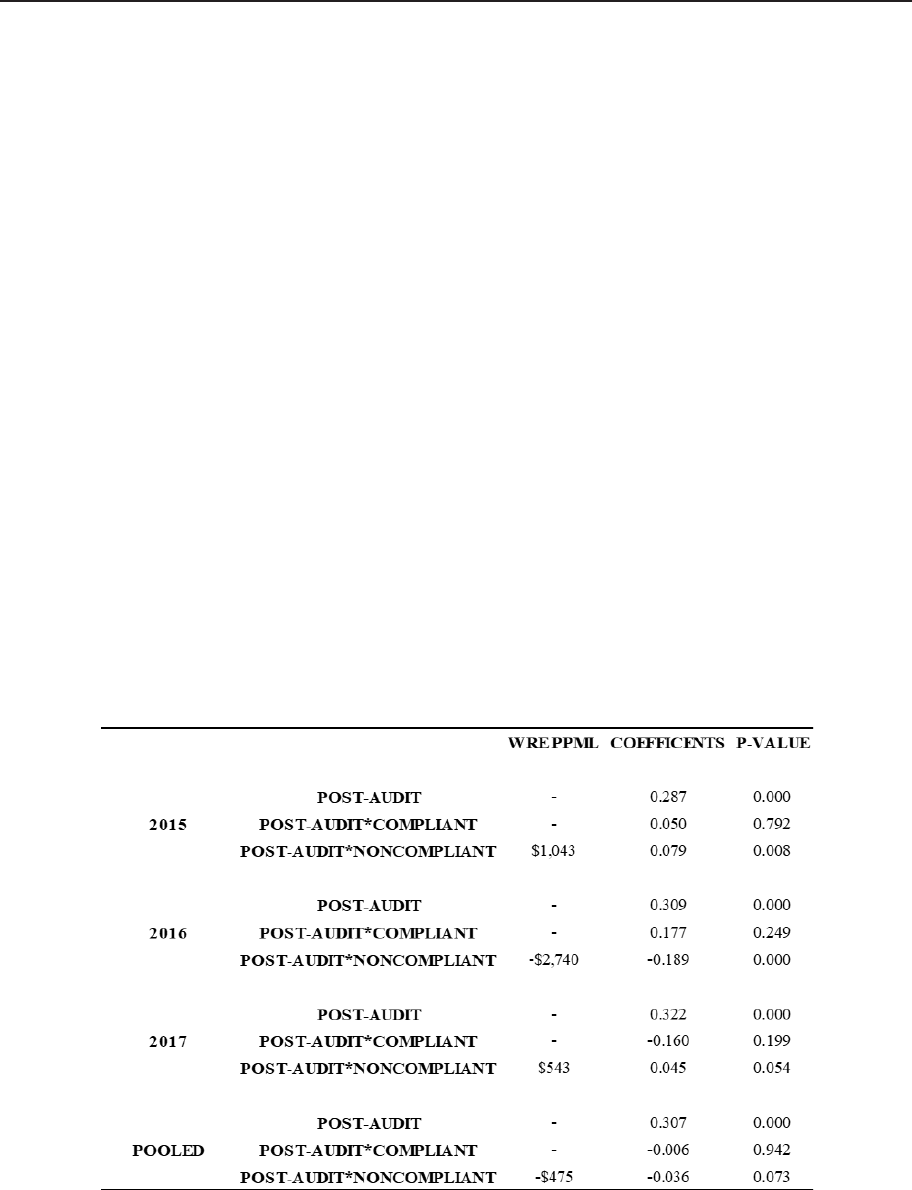
Besnek and Partington
deterrent eect, which we conrm by comparing the results to the standard DID model that can be computed
without the need of a regression. We report each nancial year independently, but we base our nal conclu-
sions on the coecients acquired from the pooled estimates for the reason that they have more observations
and combining the nancial years do not seem to violate any of the assumptions of the model. e coecients
in the tables are in percentage form, and to compute the wider revenue eects (WRE), we multiply these coef-
cients by the average pre-audit net tax amounts of the population.
i. Individuals Not in Business
Table presents the results for the INIB population. Recall from Section that the average audit yield is
equal to $1,071 in 2015, $1,098 in 2016 and $881 in 2017. If we use the pooled dataset, the average audit
yield equals$1,018. e average direct deterrent eect for noncompliant taxpayers is equal to $1,043 in 2015,
-$2,740 in 2016, and $543 in 2017. If we use the pooled dataset, the average direct deterrent eect for noncom-
pliant taxpayers is -$475. Due to the small sample size, we are unable to provide a reliable estimate of the direct
deterrent eect for compliant taxpayers. e audit treatment eects seem to remain strong over the period of
the study, with no indication of returning to the levels displayed by their control groups.
e INIB population has the smallest overall audit yield with a negative direct deterrent eect for non-
compliant taxpayers. Compliant taxpayers seem to be rare in this population (22% of the sample). e results
suggest that the intertemporal benets of the audits depend heavily on the indirect deterrent eect, as vol-
untary compliance of audited taxpayers appear to deteriorate in the post-audit years. Note that the low WRE
amounts become much larger when multiplied by the number of audited taxpayers and the years they lodge
post-audit. e audits allocated to this population should be predominantly random given the low probability
of nding large amendments (small audit yields). For this population, the use of information and edu- cational
strategies may also be more cost-eective in changing the taxpayers’ perceived probability of an audit than
running actual audits.
TABLE 2. Results for Individuals Not in Business
ii. Small Business-Individuals in Business
Table presents the results for the SB-IIB population. Recall from Section that the average audit yield is equal
to $3,914 in 2015, $2,001 in 2016 and $12,253 in 2017. If we use the pooled dataset, the average audit yield

Changes to Voluntary Compliance Following the Random Enquiry Program on Income
Tax Returns
equals $6,936. In 2016, the average direct deterrent eect for compliant taxpayers equals -$2,720. As for 2015
and 2017, we are not able provide reliable estimates. If we use the pooled dataset, the average direct deterrent
eect for compliant taxpayers equals -$1,898. e average direct deterrent eect for noncompliant taxpayers
is equal to $3,077 in 2015 and $5,554 in 2016. We are not able to provide a reliable estimate for 2017. If we
use the pooled dataset, the average direct deterrent eect for noncompliant taxpayers equals $2,616. e audit
treatment ef- fects seem to remain strong over the period of the study, with no indication of returning to the
levels displayed by their control groups.
e SB-IIB population has the largest overall audit yield with the direct deterrent eect depending on the
compliance of the treated population. Voluntary compliance of compliant taxpayers deteriorates, while non-
compliant taxpayers improve. Audits in this population should be mainly risk-based for two reasons: () it is
likely to uncover large amendments if the selection model is developed correctly; and () to avoid the risk of
randomly choosing compliant taxpayers that can worsen voluntary compliance. e intertemporal benets of
audits have the potential to be large for this population, provided that the treated include a large percentage of
noncompliant taxpayers.
TABLE 3. Results for Small Business-Individuals in Business
iii. Small Company
Table presents the results for the SB-SC population. Recall from Section that the average audit yield is equal
to in , , in and , in . If we use the pooled dataset, the average audit yield equals
,. e average direct deterrent eect for compliant taxpayers is equal to , in , $4,981 in 2016 and
$5,529 in 2017. If we use the pooled dataset, the average direct deterrent eect for compliant taxpayers equals
$4,848. In 2016, the average direct deterrent eect for noncompliant taxpayers equals $18,130. As for 2015 and
2017, we are not able provide reliable estimates. If we use the pooled dataset, the average direct deterrent eect
for noncompliant taxpayers equals $5,955. e audit treatment eects seem to remain strong over the period
of the study, with no indication of returning to the levels displayed by their control groups.
In the small business population, SB-SCs provide a lower overall audit yield than SB-IIBs. Given the costs
of running audits on companies, this is not a favourable result; especially if we want to increase audits on SB-
SC taxpayers. However, the positive direct deterrent eect more than makes up for the lower audit yield. e
SB-SC population displays the largest improvement in voluntary compliance following audits. Both compliant
and noncompliant taxpayers have large positive treatment eects. Audits allocated to this population can be

Besnek and Partington
random if preferred, as there seems to be no risk of worsening voluntary compliance due to poor selection.
Although, there is no valid reason to believe that risk-based audits would perform dierently.
TABLE 4. Results for Small Business-Small Company
5. Conclusion
is paper shows that audits on income tax returns in the REP conducted by the ATO alters taxpayers’ percep-
tions of the probability of being audited. is in turn, for better or worse, changes the future voluntary compli-
ance of taxpayers depending on the type (compliant or noncompliant) and which population (INIB, SB-IIB or
SB-SC) from which they are chosen. Understanding the direct deterrent eects of audits is important because
it quanties the intertemporal benets (costs), which subsequently helps the ATO make better decisions when
choosing between dierent compliance activities, and how to allocate resources across dierent populations.
By comparing the treated and untreated taxpayers from the INIB, SB-IIB, and SB-SC populations, we es-
timate the change in voluntary compliance that occurs in the periods immediately aer a taxpayer is audited.
e results highlight the fact that audits inuence future taxpayer behaviour, and that separate population
types respond to them dierently. It also underlines the importance of separating the responses of compliant
and noncompliant taxpayers. We nd that noncompliant taxpayers in the INIB population have a negative
direct deterrent eect. In comparison, we nd that noncompliant taxpayers in the SB-IIB and SB-SC popula-
tions have a positive direct deterrent eect. Due to the small sample size, we are not able to obtain statistically
signicant estimates for compliant taxpayers in the INIB population. We nd that compliant taxpayers in the
SB-IIB (SB-SC) population have a negative (positive) direct deterrent eect. All the audit treatment eects
seem to remain steady during the period covered by the study. e indirect deterrent eect is beyond the scope
of this paper.
e INIB (SB-IIB) population has the smallest (largest) overall audit yield. For the INIB population, in-
formation and educational strategies may be more suitable than running actual audits. Audits allocated to this
population should be predominantly random, as the intertemporal benets of audits will rely heavily on the
spillover eects on non-audited taxpayers. As for the SB-IIB population, audits should be mainly risk-based
to uncover the large, misreported liabilities in the population, and to avoid the risk of randomly choosing
compliant taxpayers to worsen voluntary compliance. e audits allocated to the SB-SC population can be

Changes to Voluntary Compliance Following the Random Enquiry Program on Income
Tax Returns
random or risk-based, as there seems to be no risk of worsening voluntary compliance due to poor selection.
Both compliant and noncompliant taxpayers have large positive treatment eects.
Lastly, instead of truncating the datasets by removing all the observations where the dependent variable
equals zero or trying to correct for the biasedness of a log-transformed dependent variable, we use a PPML
estimator which can better handle the observations where the dependent variable equals zero. Our upcoming
research will involve incorporating the 2018 REP dataset to this study. In addition, we may attempt to test the
risk-based audits to see if they change the results. Developing a model that can estimate the indirect deterrent
eect is also on the agenda.

Besnek and Partington
References
Advani, A., W. Elming, and J. Shaw (2019). “e Dynamic Eects of Tax Audits.” CAGE Online Working Paper
Series 414, Competitive Advantage in the Global Economy (CAGE).
Beer, S., M. Kasper; E. Kirchler; and B. Erard (2015). “Audit Impact Study.” National Taxpayer Advocate 2015
Annual Report to Congress, Volume 2: TAS Research and Related Studies, Washington, DC, pp. 67–99.
Bergolo, M., R. Ceni, G. Cruces, M. Giaccobasso, and R. Perez-Truglia (2020). “Tax Audits as Scarecrows:
Evidence from a Large-Scale Field Experiment.” NBER Working Paper Series, 23631.
Correia, S., P. Guimarães, and T. Zylkin (2019). “ppmlhdfe: Fast Poisson Estimation with High-Dimensional
Fixed Eects.” arXiv e-prints.
Gemmell, N. and M.Ratto (2012) “Behavioural Responses to Taxpayer Audits: Evidence From Random
Taxpayer Inquiries.” National Tax Journal, Vol. 65(1), pp. 33-58.
Slemrod, J. (2019). “Tax Compliance and Enforcement.” Journal of Economic Literature, 57, 904–54.
Gourieroux, C., A. Monfort, and A. Trognon (1984). “Pseudo Maximum Likelihood Methods: Applications to
Poisson Models.” Econometrica, 52(3): 701–20.
Silvia J.M.C., and S. Tenreyro (2006). “e Log of Gravity.” e Review of Economics and Statistics, 88(4):
641–658.

e Long-Term Impact of Audits on
Nonling Taxpayers
1
India Lindsay, Jess Grana, and Alexander McGlothlin (MITRE), Alan Plumley (IRS, RAAS)
1. Introduction
Based on current estimates, nonling taxpayers contribute %, or billion, towards the individual income
tax gap (IRS ()). In recent years, there has been an increase in the number of potential nonler cases and a
simultaneous decline in resources allocated to audit these taxpayers. e resulting decline in audit rate is cor-
related with a loss of direct revenue from nonler audits (the assessed taxed owed, interest, and penalties from
audited taxpayers). However, little is known about the long-term or indirect eect of audits on this group of
taxpayers and whether consistent declines in audits have resulted in lower voluntary compliance. is paper
considers nonling taxpayers with at least , in reported income and estimates the indirect eect of
Field (in-person) audits on their future ling behavior.
e IRS Small Business/Self Employed (SBSE) division conducts audits of nonling taxpayers. ese in-
person audits are comprehensive and likely to leave a lasting impression on audited taxpayers that may alter
their future compliance behavior. We use administrative data from the IRS for Tax Years (TYs) - on
audited nonling taxpayers to compare their behavior over time to a group of eligible-but-unaudited taxpayers.
is research will enhance the IRS’s ability to eciently allocate audit resources, inform policymakers of
the impact of the IRS’s eorts to promote compliance, and contribute towards the literature on tax policy by
highlighting the factors inuencing the ling behavior of nonlers. is is ongoing work. In addition to the
impact of audits on ling behavior, future work is planned to evaluate the impact on reported total tax. e
paper is organized as follows: Section summarizes the relevant literature, Section describes the audit selec-
tion process for nonler Field audits, Section describes our data, Section lays out the estimation approach,
Section presents results, and Section concludes.
2. Literature Review
e literature on nonlers primarily seeks to understand nonenforcement-related determinants of ling, such
as a taxpayer’s employment situation and demographic characteristics. Most of the literature studies the gen-
eral nonling population and does not focus specically on taxpayers earning more than ,, who typi-
cally have more complex tax situations than the median earning taxpayer, but a clear requirement to le a
tax return. Further, to our knowledge, only three papers in the nonler literature evaluate the eect of past
enforcement on future ling behavior.
2.1 Determinants of Nonling
For this study, we dene nonlers as taxpayers with a ling obligation who fail to le a return. Prior studies
nd that taxpayers with more easily concealed income are more likely to be nonlers (Erard and Ho ()).
For example, taxpayers with Schedule C business income and those employed in certain occupations (such
as mechanics and helpers) were the least likely to le. Taxpayers working in industries such as construction,
extraction, and production were the most likely to le. e authors nd that nonling behavior is persistent;
those who fail to le tend to continue to do so, and vice versa.
1
Approved for Public Release; Distribution Unlimited. Public Release Case Number 23-2728. is paper was produced for the U. S. government under Contract
Number TIRNO-99-D-00005, and is subject to Federal Acquisition Regulation Clause 52.227-14, Rights in Data—General, Alt. II, III and IV (DEC 2007)
[Reference 27.409(a)]. No other use other than that granted to the U. S. government, or to those acting on behalf of the U. S. government under that Clause is
authorized without the express written permission of e MITRE Corporation. ©2023 e MITRE Corporation.

Lindsay, Grana, McGlothlin, and Plumley
e persistence of nonling behavior also extends to the timeliness of ling. Erard et al. () nd that
individuals who le in the prior year are percentage points more likely to le in a timely manner the next
year than those who do not. Certain demographic characteristics, such as older age and higher income, are
associated with timely ling, while taxpayers with a higher ling burden, who are married, and who have in-
come near the ling threshold are less likely to le on time. Furthermore, they nd that taxpayers eligible for
refundable credits are more likely to le and that there is regional variation in ling compliance.
e literature on nonling behavior identies additional determinants of ling behavior: whether the
taxpayer lives in a state that taxes individual income, the number of third-party forms reported to the IRS for
the taxpayer, and their number of dependents. Other literature points to more abstract determinants of l-
ing, such as a taxpayer’s perception of government and sense of moral duty (Santoro et al. (); Gangl et al.
(); Robson et al. ()).
2.1.1 Higher Earning Nonlers
Erard et al. () model higher earning taxpayers separately and nd that taxpayers with investment, retire-
ment, and self-employment income are less likely to le than those with wage income alone. Langetieg et al.
() reach a similar conclusion. Erard et al. () also identify persistence in the ling behavior of higher-
earning nonlers, like the general nonler population.
2.2 Indirect Eects of Enforcement
To our knowledge, only three studies exist on the indirect eects of enforcement on nonlers. One study,
conducted in collaboration with the Bank of Greece, estimates the direct and indirect eects of audits of high
wealth individuals and nonlers (Tagkalakis ()). e paper nds that a % increase in the number of audits
increases direct revenue by .% and indirect revenue by .%. A drawback of this paper is that the authors
lack access to return-level data so can conduct their analysis only at the aggregate level.
Datta et al. () estimate the eect of certain IRS enforcement activities on future ling behavior by
evaluating nonler cases treated by the Automated Substitute for Return (ASFR) program. Compared to Field
audits of nonlers, ASFR handles a much larger volume of cases and works cases with simpler returns and a
lower balance due. Datta et al. () nd that ASFR treatment increases the likelihood of ling by , , and
percentage points in the through years post treatment. ey also cite past compliance behavior as an
important predictor of future compliance.
Herlache et al. () consider the impact of various mailed reminder-to-le notices on nonlers’ prior-
year noncompliance and future ling behavior, from TYs –. is research observes a .% increase in
ling of past noncompliant returns from TY , a .% increase in ling of returns for TY , and a .%
increase in ling of returns for TY . e impact of treatment on ling behavior was stronger for nonlers
(taxpayers exhibiting continuous nonling behavior) compared to stoplers (compliant taxpayers predicted to
be at risk of becoming a nonler in future years).
Overall, there is a gap in the literature analyzing both the behavior of higher-earning nonlers and the role
of IRS enforcement on ling behavior. In fact, Langetieg et al. () cite the need for a longitudinal study of
ling behavior using individual level IRS data. is research aims to begin to ll this gap.
3. Background on Audit Selection
In-person audits on nonlers are conducted by either tax compliance ocers or revenue agents who work in
the SBSE division at the IRS. e Individual Master File (IMF) Case Creation Nonler Identication Process
(CCNIP) is the selection process for identifying the majority of nonling taxpayers eligible for SBSE Field au-
dit. Nonlers may also be selected for audit via alternate processes, such as referral programs. For this research,
the CCNIP selection process was obtained through interviews with SBSE ocials.
First, the Information Returns Program (IRP) compiles reported income information from third par-
ties for all taxpayers. Forms reported by third parties include wages, tips, and other compensation paid to

e Long-Term Impact of Audits on Nonling Taxpayers
employees and reported to the IRS by their employers, in addition to forms furnished to the IRS from other
entities, such as banks, and other nancial institutions. is IRP information is combined with available infor-
mation from taxpayers’ prior tax returns to estimate total income.
If a taxpayer is identied to likely have a tax liability yet has not voluntarily led a return, the Return
Delinquency Program may initiate the process of notifying the taxpayer. Up to two notices may be sent to
the nonling taxpayer, informing them of their delinquency in ling and requesting their tax return. If the
taxpayer responds to either of these letters, their return may be accepted as led or their case is assigned to an
auditor to verify information. Taxpayers who remain as nonlers are grouped into the Taxpayer Delinquency
Investigations (TDI) inventory. e IRS applies screening criteria and may distribute TDI taxpayers, based on
specic taxpayer and tax return characteristics, to one of three enforcement functions: ASFR, Collection, or
Field audit. To be eligible for Field audit, taxpayers typically must have an estimated tax liability above an IRS-
specied threshold and total reported income typically exceeding ,.
e SBSE Field oce receives the lists of eligible TDI cases, estimates everyone’s tax liability, and assigns
a priority score. e priority score is a function of the taxpayers’ estimated balance due and the likelihood of
securing the balance due. Cases are assigned codes specic to the type of audit required, sorted by region, and
ranked by priority. Top priority cases are sent to regional eld oces and assigned to tax auditors according to
each region’s workplan and available resources. In addition to auditing nonling TDI cases, Field audits may
be conducted on returns that are led in response to delinquency notices and meet selection criteria.
4. Data
4.1 Sample Construction
is study uses taxpayer and audit record data obtained from the IRS Compliance Data Warehouse (CDW) us-
ing primary Taxpayer Identication Numbers. e treatment group consists of nonling taxpayers in the TDI
Lists workstream who were subject to audits between TYs to and is compared to a control group
that consists of taxpayers who were not audited but were in the TDI Lists workstream during the same period.
Each taxpayer is assigned a “baseline year” that is dened as the tax year the taxpayer entered the sample, ei-
ther because they were audited in that tax year (treatment group) or because they were eligible-but-unaudited
in that tax year (control group). We analyze these taxpayers’ tax reporting behavior years before this baseline
year through years aer, creating a dataset measuring taxpayer behavior from –.
4.1.1 Treatment Group
e treatment group consists of all nonling taxpayers audited from the TDI Lists workstream during the
baseline period (TYs –). Data on taxpayers audited from TDI Lists were obtained from IRS audit
record data. We include the primary returns selected for audit in each tax year and exclude “pickups”—returns
from the same taxpayer for other tax years that were audited because of the primary audit.
4.1.2 Control Group
e control group includes unaudited nonlers identied by CCNIP during TYs –. Taxpayer data
were extracted from the CCNIP database using queries designed to replicate the SBSE screening criteria for
this population. We veried income, tax due, and ling status to ensure taxpayers met the primary selection
criteria. e control group excludes taxpayers who led late, were secondary lers, or who led in response to
a delinquency notice in the baseline year.
4.1.3 Sample Cleaning
Among audited taxpayers, we drop those with missing or unmatched audit record data. We also remove tax-
payers who were selected for audit outside of the CCNIP process (such as the State Audit Reporting Program
and various referral programs). Because we exclusively source the control group from CCNIP, we do so for the
treatment group as well. Our sample contained audited taxpayers that had a baseline year tax return on le.

Lindsay, Grana, McGlothlin, and Plumley
ese individuals either led a Form for the tax year of the audit prior to audit start or led in response
to delinquency notices. Regardless of late ling, these individuals may still have been audited by the nonling
Field audit group if their return met selection criteria. ese individuals are dropped from the sample.
Among the control group, taxpayers with audits in the years before and aer baseline are dropped from
the sample so we estimate the impact of the baseline audit only. We also remove any taxpayers in the control
group that were identied by CCNIP but later deemed not to have a tax liability.
For both the treatment and control groups, taxpayers are removed from the sample if they died within
years of their baseline year. During the – period, some taxpayers were candidates for audit in mul-
tiple baseline years. To assign each taxpayer only one baseline year, we applied de-duplication rules. Taxpayers
audited more than once are assigned their rst audit year as their baseline year. Taxpayers considered eligible
more than once (but never audited during our baseline period) are also assigned their rst eligible year as their
baseline year. Taxpayers appearing in both the treatment and control group during this period are assigned to
the treatment group with their rst audit year as their baseline year.
4.2 Dependent Variable
Our model’s dependent variable is fact of ling, a binary variable that equals if the taxpayer les a return and
otherwise. is variable is created for each taxpayer in our sample for the years preceding their baseline
year to the years following. For baseline years, all taxpayers in our sample have a fact of ling equal to , by
denition. We construct fact of ling for o-baseline years by consolidating ling information on a taxpayer
from the Information Returns Transaction File (IRTF). For a given tax year, a taxpayer is considered to have
led if they led a Form (timely or late), is listed as a secondary ler on another taxpayer’s Form , is
selected for a nonling audit but is later deemed to not have a tax liability, or is selected for a nonling audit
but led prior to the audit.
A taxpayer has fact of ling set to if they are a known nonler or a “ghost.” In the context of this study,
the term nonler refers to a taxpayer who was identied by CCNIP as having a tax liability but did not volun-
tarily le a return. e term nonler includes nonling taxpayers experiencing a nonler audit or some other
treatment by an IRS nonler program. ough these individuals may le in response to treatment, their fact
of ling is not voluntary. A “ghost” refers to a taxpayer who did not le and is not a known nonler for a given
tax year. A taxpayer could become a ghost via two mechanisms:
1. e taxpayer does not have enough income to have an income tax liability. is could occur if a taxpayer
suddenly becomes unemployed and has no income. If the taxpayer had no income to report to the IRS
(either by themselves or by third parties), they would not appear in IRS records.
2. e taxpayer has income but does not report the income and it is not covered by third-party reporting.
is could occur if a taxpayer is self-employed, and the IRS does not have a means of verifying a tax
liability in advance of an audit.
Since taxpayers in either case would not be in IRS records, we cannot distinguish between the rst case
(no tax liability) and the second case (owes taxes); all we know about them is that they were nonlers in the
baseline year and in an o-baseline year, they did not le, and they were not identied by the IRS as a non-
ler. Based on conversations with nonler subject-matter experts in the IRS Research, Applied Analytics, and
Statistics organization, we made the decision to assume ghosts were nonlers. is assumes that income for
higher earning nonlers tends to be persistent and that such taxpayers are more likely to conceal their income
than to have no income.
4.3 Independent Variables
In addition to audit status, we control for characteristics identied from prior literature as important determi-
nants of the decision of whether to le. ese include demographic and nancial information, as well as past
ling behavior. In the current model, control variables come from the CCNIP database and are time-invariant
because they are derived solely from baseline year data. is approach was chosen because taxpayers in our

e Long-Term Impact of Audits on Nonling Taxpayers
dataset tend to become ghosts, meaning o-baseline year data are not always available. In future research, we
hope to overcome this barrier by compiling time-varying control variables from a variety of data sources.
4.3.1 Demographic Variables
We control for taxpayer level demographics, including Census region of residence,
whether the taxpayer
resides in a state taxing individual income, whether the taxpayer was over in the baseline year, whether
the taxpayer was under in the baseline year, and their ling status in the prior year. We treat ling status
as a binary variable, with being Married Filing Jointly and the reference level being other ling statuses
(Single, Married Filing Separately, Widow/er, Head of Household) collapsed into one category. We also in-
clude an indicator for whether the taxpayer claimed the Earned Income Tax Credit (EITC) in the prior year.
Unfortunately, we are inconsistent with prior literature in that we have not yet controlled for the number of
dependent children, which is not in the CCNIP database.
4.3.2 Financial Variables
We further construct a set of variables related to the taxpayers’ nancial status. Total IRP income is dened as
the sum of all income reported on third-party forms, without subtracting possible losses or deductions. We
also construct an indicator for whether the taxpayer met the , threshold in the baseline year, since
some taxpayers in the treatment group did not.
We also include the number of IRP forms submitted by third
parties to the IRS, since this captures both the ling burden felt by the taxpayer and the complexity of income
sources, and because each additional report to the IRS from third parties increases the “visibility” of that
taxpayer.
We include the dierence in income between the prior year and the baseline year. Changes in income
have not been considered by the previous nonling literature but help to capture the volatility of taxpayer in-
come. It also serves as an indicator of one source of potential nancial burden that may alter ling behavior. A
positive value indicates the taxpayer’s reported income grew in their baseline year compared to the prior year.
Additionally, we construct indicators to capture the presence of various income sources listed on third-party
documents, including self-employment income,
investment income,
retirement income,
broker transaction
income,
as well as other types of reported income.
4.3.3 Past Filing Behavior Variables
Lastly, we construct variables related to taxpayers’ past compliance behavior. ese variables include whether
the taxpayer led in the prior year, whether the taxpayer was a ghost in the prior year, and whether the tax-
payer was audited in the years prior to baseline. We also control for the operational priority score, an IRS-
internal metric used to rank taxpayers for audit selection.
4.4 Data Summary
Our nal sample includes a total of , taxpayers in the treatment group and , taxpayers in the con-
trol group. Figure summarizes sample size by baseline year. While the control group grows throughout the
sample period, the treatment group remains around taxpayers in , , , and but increases
in size in and . During this time period, the overall number of potential nonler cases in CCNIP
increased from . million in to . million in .
2
Census region of residence was determined from the state derived from the taxpayer’s address line or ZIP code, listed on third-party forms. If Census region of
residence was not present, region was set to “None.”
3
By sample design, all taxpayers in our control group met the $100,000 threshold in the baseline year.
4
Self-employment income is restricted to the types of self-employment income required to be reported to the IRS by third parties: barter income, crop insurance,
attorney fees, shing income, medical payments, nonemployee compensation, and patronage income.
5
Investment income includes income from distribution shares (Schedule K1), dividends (Schedule 1099-DIV), interest income (Schedule 1099-INT), and passive
income (Schedule K1).
6
Retirement income includes pension and Social Security payments.
7
Broker transaction income is dened as income from mediating the sale or purchase of property, services, or investments (Schedule 1099-B).
8
Other income is dened as income reported on Schedule 1099-MISC, real estate and rental income, lottery income, and business income.
9
A glitch in CCNIP computer processing occurred in 2012, resulting in a drop in the total nonling taxpayers identied in that year.

Lindsay, Grana, McGlothlin, and Plumley
FIGURE 1. Sample Size by Baseline Year
Figure plots the distribution of the priority score for the treatment and control groups. While the audited
group includes many more taxpayers with a priority score of and above, there is common support in prior-
ity scores across both groups. is provides evidence towards the validity of our sample construction.
FIGURE 2. Distribution of Priority
Note: Priority is truncated for readability.

e Long-Term Impact of Audits on Nonling Taxpayers
Figure plots the distribution of audit start date and end date for the treatment group. e majority of
audits start – years aer the baseline year and end – years aer the baseline year. Given this distribution of
audit timing, we would not expect to see an indirect eect from an audit until at least years aer the baseline
year.
FIGURE 3. Audit Timing
Note: Audit timing is truncated for readability.
Table summarizes the control variables in our model for the treatment and control groups. As men-
tioned above, all control variables are sourced from the CCNIP database at the relevant baseline year. Dollar-
denominated variables (Total IRP Income and Income Dierence from PY) are adjusted to reect U.S.
dollars, scaled by ,. In terms of demographic characteristics, most taxpayers in both groups are be-
tween the ages of and , have a ling status of single/other, and reside in a state taxing income. In terms
of nancial characteristics, most taxpayers in our sample earned more reported income in their baseline year
than in the prior year (about , more for both groups). Taxpayers selected for audit have an average of
IRP documents compared to about for the control group. Most taxpayers in the control group have in-
vestment income present and the majority of taxpayers in the treatment group have self-employment income.
Considering past ling behavior, about % of the treatment group led in the prior year while about %
of the control group did so. More than half of the treatment group were audited prior to their baseline year,
although this variable captures audits of any kind (not just TDI Lists audits). e largest dierences between
groups occur in the baseline priority score, whether the taxpayer met the , threshold for reported in-
come, and whether a taxpayer was audited in the years prior to baseline year.

Lindsay, Grana, McGlothlin, and Plumley
TABLE 1. Summary Statistics for Treatment and Control Variables, TYs 2009–2014
Variable
Mean for Treatment
Group
Mean for Control Group
Demographic Variables
Census Region
East North Central 11% 8% 3%
East South Central 7% 4% 3%
Mid Atlantic 12% 12% 0%
Mountain 7% 7% 0%
New England 5% 4% 1%
Pacic 15% 16% 1%
South Atlantic 17% 20% 3%
West North Central 4% 3% 1%
West South Central 20% 16% 4%
Not Available 1% 11% 10%
Income Tax State 73% 75% 2%
Over 65 5% 7% 2%
Under 30 7% 13% 6%
PY Filing Status
Single/other 70% 85% 15%
Married ling jointly 30% 15% 15%
PY EITC 9% 4% 5%
Financial Variables
Total IRP Income $5.71 (45.91) $5.62 (28.23) $0.09
$100,000 Threshold Indicator 54% 100% 46%
Number of IRP Forms 36.06 (232.96) 44.84 (183.65) 8.78
Income Dierence from PY $4.97 (46.36) $5.02 (29.16) $0.05
SE Income 69% 45% 24%
Investment Income 45% 72% 27%
Retirement Income 21% 21% 0%
Broker Transaction Income 19% 35% 16%
Other Income 29% 59% 30%
Past Filing Behavior Variables
Filed in PY 39% 50% 11%
Ghost in PY 6% 20% 14%
Any Audit Last 6 TYs 53% 4% 49%
Baseline Priority 727 (166) 650 (163) 77
Note: Dollar-denominated variables (Total IRP Income and Income Dierence from PY) are expressed in terms of 2018 dollars and are scaled by $100,000. The stan-
dard deviation for continuous variables is displayed in parenthesis. Other than Baseline Priority and Number of IRP forms, all variables reect percentages.

e Long-Term Impact of Audits on Nonling Taxpayers
5. Methodology
Our main methodological approach estimates a linear probability model of a taxpayer’s fact of ling in an
event-study type model.
is model species taxpayer i’s ling behavior in year t as follows:
Audit is a time-invariant variable set to for the treatment group and for the control group. e coef-
cient on Audit measures the dierence in the average ling behavior across the treatment and control groups
in all years. Year from baseline is a set of indicator variables that separately control for fact of ling behavior
across both groups for each year, years pre-baseline through years post-baseline. e baseline year is the
reference category and is excluded from the regression.
e primary regressors of interest are the interactions between Audit and Year from Baseline. is set of
variables captures the time path of ling compliance for the audited group. We hypothesize that the estimates
in pre-baseline years will be negative, indicating decreased ling compliance up to the baseline year, and that
estimates in post-baseline years (beginning in the nd or third year from baseline) will be positive. is would
indicate that audits increase the likelihood of subsequent ling and aligns with audit start dates (Figure ).
Finally, consistent with prior literature on indirect eects, we expect estimates to attenuate over time in the
post-baseline period.
Taxpayer Controls are the set of demographic, nancial, and ling behavior variables discussed in Section
.. ese variables are drawn from baseline year CCNIP data and are time-invariant. Finally, Tax Year is a set
of xed eects capturing yearly uctuations in fact of ling common across all taxpayers in our sample.
6. Results
6.1 Descriptive Analysis
Figure visualizes the distribution of the Fact of Filing variable by year from baseline for taxpayers in the treat-
ment and control groups. For the treatment group, the proportion of taxpayers ling a return decreases in the
years leading up to audit and increases until the th year aer the audited Tax Year. For the control group, the
proportion of taxpayers ling a return remains around % in years ve through two prior to baseline and
decreases in the years leading up to the baseline year. Aer the baseline year, the proportion of taxpayers in
the control group ling remains between –%. Despite slight dierences in the proportion of taxpayers l-
ing in either group, the treatment and control groups exhibit similar ling behavior in the years leading up to
baseline. By the construction of our sample design, no taxpayer in either group led a return in their baseline
year. ese plots suggest that:
• Taxpayers in both groups trend towards delinquency in the years prior to baseline;
•
–
•
baseline).
t
( 1 )
10
A linear probability model was selected for its interpretability, although we plan to explore alternate specications (e.g., logistic regression) in future work.

Lindsay, Grana, McGlothlin, and Plumley
FIGURE 4. Taxpayers Filing Over Time
Figure plots the distribution of ghost taxpayers in the control group (whom we consider as nonlers
in our model) and in the treatment group. e proportion of ghost taxpayers in the control group ranges
from approximately –%. A smaller proportion of ghosts are present in the treatment group. Both groups
exhibit similar trends, with the proportion of ghosts decreasing in the years leading up to baseline year and
increasing in the years following baseline year.
FIGURE 5. Ghost Taxpayers in the Treatment and Control Groups

e Long-Term Impact of Audits on Nonling Taxpayers
6.2 Econometric Analysis
In this section, we summarize results from our main model. Full results are displayed in Table .
6.2.1 Audit, Year from Baseline, and Interactions
e interaction term Audit*Year from Baseline captures the indirect eect of an audit on ling behavior; the
estimates show the time path of the fact of ling for the audited group relative to the control group. Figure
visualizes the coecients and their standard errors, for the Audit variable and the interaction terms.
Based on audit timing (Figure ) and descriptive analysis (see Figure ), we hypothesized that the indirect
eect would begin to appear in the second year from baseline. Table conrms that this eect does begin in
the second year from baseline: the audited group is .–. percentage points more likely to le in the –
years from baseline than the control group. e magnitude of this eect increases during the – years post-
baseline and decreases thereaer (an attenuation seen in much of the prior specic indirect eects literature).
e negative eect for Year from Baseline - indicates the audited group is less like to le than the control
group in the year prior to their Tax Year of audit. Besides the year prior to baseline, the insignicance of in-
teraction terms in years two and three prior to baseline and year one aer baseline suggest general similarities
in ling behavior across groups in the years surrounding baseline. Interestingly, the coecient on Audit is not
statistically signicant, suggesting that irrespective of treatment and baseline year, taxpayers in the control and
treatment groups exhibit similar ling behavior across Tax Years, on average. Finally, the positive coecients
estimated for the Year from Baseline variables indicate that both groups are more likely to le a return in o-
baseline years (i.e., the baseline year is an outlier year).
FIGURE Audit Variables.

Lindsay, Grana, McGlothlin, and Plumley
TABLE 2. Regression Results
Dependent Variable: Fact of Filing
Variable
Parameter
Estimate
Standard
Error
Audited 0.015 (0.012)
Year from Baseline-5 0.622*** (0.015)
Year from Baseline-4 0.635*** (0.014)
Year from Baseline-3 0.648*** (0.014)
Year from Baseline-2 0.615*** (0.014)
Year from Baseline-1 0.518*** (0.013)
Year from Baseline+1 0.306*** (0.013)
Year from Baseline+2 0.338*** (0.014)
Year from Baseline+3 0.353*** (0.014)
Year from Baseline+4 0.379*** (0.014)
Year from Baseline+5 0.398*** (0.015)
Year from Baseline+6 0.389*** (0.016)
Year from Baseline+7 0.41*** (0.016)
Year from Baseline+8 0.434*** (0.017)
Audited*Year from Baseline-5 0.139*** (0.016)
Audited*Year from Baseline-4 0.096*** (0.016)
Audited*Year from Baseline-3 0.018 (0.016)
Audited*Year from Baseline-2 -0.031 (0.016)
Audited*Year from Baseline-1 -0.12*** (0.016)
Audited*Year from Baseline+1 0.015 (0.016)
Audited*Year from Baseline+2 0.053*** (0.016)
Audited*Year from Baseline+3 0.123*** (0.016)
Audited*Year from Baseline+4 0.138*** (0.016)
Audited*Year from Baseline+5 0.122*** (0.016)
Audited*Year from Baseline+6 0.124*** (0.016)
Audited*Year from Baseline+7 0.1*** (0.016)
Audited*Year from Baseline+8 0.058*** (0.017)
Over 65 -0.031*** (0.006)
Under 30 -0.015*** (0.005)
PY EITC 0.033*** (0.005)
PY Filing Status = Married Filing Jointly 0.086*** (0.003)
Census Region: East South Central -0.012 (0.007)
Census Region: Mid Atlantic 0.02*** (0.006)
Census Region: Mountain -0.004 (0.007)
Census Region: New England 0.034*** (0.008)
Census Region: Not Available -0.064*** (0.008)
Census Region: Pacic 0.022*** (0.005)
Census Region: South Atlantic 0.003 (0.005)
Census Region: West North Central -0.02** (0.008)
Census Region: West South Central -0.015** (0.006)
Income Tax State -0.011*** (0.004)
Number of IRP Forms 0.000*** (0.000)

e Long-Term Impact of Audits on Nonling Taxpayers
Variable
Parameter
Estimate
Standard
Error
Broker Transaction Income
0.023*** (0.004)
Other Income
0.01*** (0.003)
Retirement Income
0.026*** (0.004)
Investment Income
0.078*** (0.003)
SE Income
-0.007** (0.003)
$100,000 Threshold Indicator
-0.026*** (0.004)
Income Dierence from PY
0.000** (0.000)
Total IRP Income
0.000*** (0.000)
Baseline Priority
0.000*** (0.000)
Any Audit Last 6 TYs
0.006 (0.004)
Filed in PY
0.218*** (0.003)
Ghost in PY
-0.073*** (0.005)
Constant
-0.239*** (0.024)
Observations
110,586
R-squared
0.211
Adjusted R-squared
0.211
F Statistics
411.224*** (df = 72; 110,513)
Note: **p<0.05, ***p<0.01.
6.2.2 Demographic Variables
Taxpayers over and under have a lower probability of ling. Taxpayers claiming EITC in the year prior
to baseline are . percentage points more likely to le in other years, and taxpayers with a ling status of
Married Filing Jointly are . percentage points more likely to le in other years. Results across Census regions
conrm prior literature ndings that compliance varies across geography. Finally, living in a state that imposes
an income tax decreases the likelihood of ling by . percentage points.
6.2.3 Financial Variables
Having certain types of income, such as broker transaction income, retirement income, investment income
and other income increases the likelihood of ling. e presence of investment income has the strongest ef-
fect compared with other types of income sources, increasing the likelihood of ling by . percentage points.
Having self-employment income decreases the likelihood of ling. However, since only certain categories of
self-employment income are covered by third-party reporting, measurement error may obscure a true positive
eect. Taxpayers who met the , threshold for reported income in their baseline year are . percentage
points less likely to le, suggesting a negative relationship between income and propensity to le. However,
other income-related variables, Income Dierence from PY and Total IRP Income, do not have an eect on the
likelihood of ling.
6.2.4 Past Filing Behavior Variables
Interestingly, a taxpayer’s priority score and the presence of any type of audit in the years prior to baseline
do not have an eect on the probability of ling. Taxpayers who led a return in the year prior to baseline are
. percentage points more likely to le in other years. If the taxpayer is a ghost in the year prior to baseline,
their expected probability of ling in other years decreases by . percentage points. Together, these estimates
suggest there is persistence in ling behavior.
TABLE 2. Regression Results (Continued)
Dependent Variable: Fact of Filing

Lindsay, Grana, McGlothlin, and Plumley
6.3 Robustness Checks
6.3.1 Denition of Ghosts
Our construction of the fact of ling variable assigns ghosts to the nonling status on the assumption that
individuals who did not le and do not have third-party reported income still have a tax liability. We explore
the validity of this assumption by rerunning our regression, labeling ghosts as fact of ling = . Table in the
Appendix contains the regression results.
Figure compares the coecients and standard errors for Audit variables between the linear probability
model categorizing ghosts as fact of ling = (Table ) and the linear probability model categorizing ghosts
as fact of ling = (Table ). e relationship between Audit and Year from Baseline on a taxpayer’s fact of l-
ing is smaller, although similar trends are observed. e negative eect for Audit*Year from Baseline values of
- through indicates the audited group is less likely to le in all years leading up to knowledge of the audit
start, compared to the control group. While an indirect eect of an audit on a taxpayer’s future ling behavior
is observed, it is signicant only in years and from baseline, with an expected increase in the likelihood of
ling ranging from .–. percentage points.
By changing this assumption, the Audit variable becomes statistically signicant at the -percent level,
indicating taxpayers in the audited group are . percentage points more likely to le across all years. Likewise,
the presence of any audit in the years prior to baseline now has a negative and signicant eect. e relation-
ship between whether a taxpayer was a ghost in the year prior to baseline and their ling behavior across all
years changes to a positive relationship, increasing the likelihood of ling by percentage points. e inu-
ence of a taxpayer’s ling in the year prior to baseline decreases, while still being positive.
Overall, the magnitude and levels of our estimates are sensitive to the denition of ghost taxpayers,
however, the trends and overall takeaways seem to be consistent despite dierent assumptions around these
taxpayers.
FIGURE Audit Variables Depending on the
Audited
Audited*Ye
ar
Fro
m Bas
eli
ne
-5
Aud
ite
d*Ye
ar
Fro
m Bas
eli
ne
-4
Aud
ite
d*Y
ear
Fr
om
B
aseline -3
Audited*Year Fr
om Baseline -2
Audited*Year Fr
om Baseline -1
Audi
ted*Yea
r F
rom
Baselin
e 1
Audited*Yea
r Fr
om Baseline 2
Audit
ed*Year
Fro
m Base
line 3
Audi
ted*Year F
rom Baseline 4
Audited*Year
From Ba
seli
ne 5
Audite
d*Ye
ar From B
aseline 6
Audited*Year From B
aselin
e 7
Audited*Year From Baseline 8
G
hos
t labeled as Filing = 0
Gho
st l
abeled as Fi
ling =
1

e Long-Term Impact of Audits on Nonling Taxpayers
7. Discussion
Understanding nonling behavior is dicult due to the inherent lack of information about these taxpayers. It
is especially curious why higher earning nonlers do not le a return, given that they may be more visible to
the tax authority and because they are identied by third party data as potentially owing substantial taxes. As
our analysis reveals, taxpayers who do not le a return oen fail to do so in other years as well. ese challeng-
es require creative approaches to sample selection and model design to analyze these taxpayers’ fact of ling.
In this paper, we provide one of the rst attempts to understand the role of audits on future ling of audited
nonlers—a contribution to the nonling literature, which has largely focused on the role of non-enforcement
related ling determinants.
Our results indicate that in-person audits of nonlers improve subsequent ling compliance. Nonlers
subject to a Field audit are .–. percentage points more likely to le in the – years aer baseline (i.e.,
the tax year of the audited return), compared to similar but unaudited taxpayers. is eect peaks in the
th
year aer baseline. is nding is qualitatively similar to ndings from other studies on the eect of audits on
future tax compliance.
e sensitivity analysis on our assumption of ghosts owing a tax liability conrms the presence of an in-
direct eect irrespective of our assumption. However, if all ghosts in our sample are missing from IRS records
because they do not have a tax liability, our estimates of an indirect eect are overstated.
is study also sheds light on the relationship between prior and future ling behavior. Taxpayers who
led in the year prior to baseline year are . percentage points more likely to le in other years (regardless
of being audited). On the other hand, taxpayers who were unable to be identied through IRS data processes
(ghosts) in the year prior to the baseline year are . percentage points less likely to le in other years.
7.1 Comparison with Other Research
We compare our contributions to other research estimating the inuence of IRS treatment on nonling tax-
payer’s ling behavior.
Datta et al. () modeled the ling behavior of nonlers over a -year period aer treatment by the
ASFR program between TYs and . e ASFR program similarly treats nonlers identied by CCNIP,
but focuses on lower income individuals with simpler returns—individuals with primarily wage income and
fewer forms reported to the IRS by third parties. e ASFR program diers from an in-person Field audit as
it treats nonlers by estimating their balance due and interacts with taxpayers via mailed correspondence. e
study estimated treatment by ASFR resulted in an , , and percentage point increase in the likelihood of
ling to years aer treatment, respectively. Comparatively, our estimated eects of a Field audit are smaller
in magnitude. However, as our study monitored ling behavior through years aer baseline, we observed an
eect persisting through the
th
year.
Herlache et. al () conducted a randomized control trial to explore the inuence of various mailed
notice programs on nonlers’ prior year noncompliance in TY and ling behavior in TYs and .
eir population similarly consisted of nonlers identied from CCNIP in TY , but did not have any
additional selection criteria from this population. Across the various treatments employed, they identied a
.% increase in ling of prior-year returns for TY and a .–.% increase in ling for current and fu-
ture returns, as a result of mailed reminder-to-ler notices. is study extended analysis to consider the role
of notices on expected stoplers, taxpayers compliant in prior years yet predicted to be at risk of becoming
noncompliant, identifying a . to . percentage increase in ling.
Both mailed reminder-to-le notices and treatment by ASFR are less expensive and require fewer re-
sources than in-person Field audits, enabling them to treat a larger population of nonlers. Despite dierences
in type of treatment, tax years, and populations considered, the impact of mailed outreach was smaller and
the impact of ASFR treatment was larger, compared with our estimates. e study by Herlache et. al ()
provides insight into the role of notices as an instrument of deterrence prior to noncompliance behavior. is
type of treatment may be an eective form of treatment when nonlers are unaware of either the need to le,

Lindsay, Grana, McGlothlin, and Plumley
the consequences from not ling, or their detectability by the IRS. Datta, et. al () illustrates the inuence of
correspondence treatment on identied nonlers. As ASFR focuses on a dierent population than Field audits,
the dierence in estimates may be indicative of higher compliance rates in lower income and single source of
income populations.
Nonling individuals audited by Field tend to owe a substantial tax liability, have complex returns, and
remain noncompliant, despite being mailed up to two delinquency notices. ese high dollar noncompliance
individuals are a strategic focus of IRS enforcement moving forward (IRS ()). Nonlers are responsible for
a substantial portion of the tax gap, and these results highlight the value of audits as a policy tool to promote
compliance. While audits of this group can be costlier than audits of simpler returns, maintaining audit cover-
age of the nonling population provides an opportunity to promote voluntary compliance as well as generate
direct revenue.
7.2 Limitations and Future Research
ere are several near-term extensions we plan to address. Foremost, we plan to estimate the eect of a non-
ler audit on total tax reported by the taxpayer in subsequent years. is extension will provide dollar-valued
estimates of the indirect eect that can be compared against direct revenue as well as the cost to the IRS of
conducting these audits. Other extensions include additional robustness checks, collecting a richer set of con-
trol variables, rening sample design, and considering a multinomial outcome variable, which are described
in more detail below.
7.2.1 Robustness Checks
To further validate model estimates and to assist with removing confounding, future work will employ propen-
sity-score matching or inverse probability weighting methods to the baseline year variables. ese techniques
will allow for an alternative and possibly more comparable treatment and control group when estimating the
casual eect of an audit.
7.2.2 Richer Control Variables
Our current analysis relies on third-party reported data available only for the taxpayer’s baseline year. is
limits the ability to control for time-varying characteristics that inuence ling behavior. Future work may
consider constructing control variables for the years leading up to the baseline year. is extension poses data
availability challenges since a signicant portion of these taxpayers are ghosts in o-baseline years.
Future work may also incorporate additional control variables not considered here. By capturing tax-
payers’ reported income in o-baseline years, we could verify the presence of a tax liability. As discussed in
Section , CCNIP and the Returns Delinquency Program issue notices to inform taxpayers of their delinquent
tax liability. Additional control variables can include whether the taxpayer received a notice and the type of
notice received. Alternatively, receiving a delinquency notice could serve as a treatment variable itself (instead
of a TDI Lists audit). We could also control for the pattern of nonling: whether the taxpayer was a one-time
nonler, a nonler with a pattern of interrupted nonling, or a nonler with a continuous pattern of nonling.
7.2.3 Sample Design
A limitation of this study is in the handling of taxpayers with multiple audits. Seventy-two percent of our treat-
ment group received at least one other TDI Lists audit in o-baseline years,
while .% experienced another
type of audit in o-baseline years. We retain these multi-audited taxpayers in the current version of our analy-
sis to preserve sample size, but audits occurring before the baseline year likely cause us to underestimate the
indirect eect of audit. Future research can include sensitivity analysis of the indirect eect on single-audited
taxpayers versus multiple-audited taxpayers.
11
Our deduplication rules assign multi-audited taxpayers to their rst year of audit within the baseline period 2009–2014. However, taxpayers assigned to baseline
year 2009 could still have been audited prior to 2009. 2,120 taxpayers had a TDI Lists audit in both the 6 years prior to baseline and 6 years post baseline. 864
taxpayers had a TDI Lists audit in the 6 years prior to baseline only, and 1,142 taxpayers had a TDI Lists audit in the 6 years aer baseline only.

e Long-Term Impact of Audits on Nonling Taxpayers
7.2.4 Multinomial Outcome
e fact of ling outcome variable captures whether a taxpayer les for a given year. However, this variable
does not capture compliance. A compliant taxpayer les voluntarily and timely. Future research can consider
a three-level outcome variable to capture the distinctions between timely ling, late ling, and nonling. is
would extend this analysis to estimate the indirect eect of a Field audit on a nonler’s future compliance.

Lindsay, Grana, McGlothlin, and Plumley
References
Datta, Saurahh, Stacy Orlett, and Alex Turk. 2015. “Individual Nonlers and IRS-Generated Tax Assessments:
Revenue and Compliance Impacts of IRS Substitute Assessments When Taxpayers Don’t File.” Internal
Revenue Service. https://www.irs.gov/pub/irs-soi/15rescondatta.pdf.
Erard, Brian and Chih-Chin Ho. 2001. “Searching for Ghosts: Who Are the Nonlers and How Much Tax Do
ey Owe?” Journal of Public Economics 81(1): 25-50. https://doi.org/10.1016/S0047-2727(00)00132-8.
Erard, Brian, Patrick Langetieg, Mark Payne, and Alan Plumley. 2020. “Ghost in the Income Tax Machinery”.
Munich Personal RePEc Archive 100036. https://mpra.ub.uni-muenchen.de/100036/.
Erard, Brian, Tom Hertz, Pat Langetieg, Mark Payne, and Alan Plumley. 2022 “To File or Not To File? What
Matters Most?”Working Paper.
Gangl, Katharina, Erich Kirchler, Christian Lorenz, and Benno Torgler. 2015. “Wealthy Tax Non-Filers in a
Developing Country: Taxpayer Knowledge, Perceived Corruption, and Service Orientation in Pakistan.” In
B. Peeters, H. Gribnau, & J. Badisco (Authors), Building Trust in Taxation (pp. 355-376). Intersentia. https://
doi.org/10.1017/9781780684734.
Government Accountability Oce. 2015. “IRS Return Selection: Certain Internal Controls for Audits in the
Small Business and Self-Employed Division Should Be Strengthened.” GAO-16-103. https://www.gao.gov/
products/gao-16-103.
Herlache, Anne, Ishani Roy, Alex Turk, and Stacy Orlett. 2019. “Enforcement Versus Outreach – Impacts on
Tax Filing Compliance” e IRS Research Bulletin Publication 1500 (Rev. 6-2020). https://www.irs.gov/pub/
irs-prior/p1500--2020.pdf.
Internal Revenue Service. 2019. “Federal Tax Compliance Research: Tax Gap Estimates for Tax Years 2011-
2013.” Publication 1415 (Rev. 09-2019). https://www.irs.gov/pub/irs-prior/p1415--2019.pdf.
Internal Revenue Service. 2022. “Federal Tax Compliance Research: Tax Gap Estimates for Tax Years 2014-
2016.” Publication 1415 (Rev. 08-2022). https://www.irs.gov/pub/irs-pdf/p1415.pdf.
Internal Revenue Service. 2023. “Internal Revenue Service Ination Reduction Act Strategic Operation Plan
FY 2023-2013.” Publication 3744 (Rev. 04-2023). https://www.irs.gov/pub/irs-pdf/p3744.pdf.
Langetieg, Patrick, Mark Payne, and Alan Plumley. “Counting Elusive Nonlers Using IRS Rather an Census
Data”. 2017. Internal Revenue Service. https://www.irs.gov/pub/irs-soi/17resconpayne.pdf.
Robson, Jennifer, and Saul Schwartz. 2020. “Who Doesn’t File a Tax Return? A Portrait of Non-Filers.”
Canadian Public Policy 46(3): 323-339. https://doi.org/10.3138/cpp.2019-063.
Santoro, Fabrizio, Edward Groening, Winnie Mdluli, and Mbongeni Shongwe. 2021. “To File or Not To
File? Another Dimension of Tax Compliance – the Eswatini Taxpayer’s Survey.” Journal of Behavioral and
Experimental Economics 95 101760. https://doi.org/10.1016/j.socec.2021.101760.
Tagkalakis, Athanasios O. 2014. “e Direct and Indirect Eect of Audits on the Tax Revenue in Greece.”
Economics Bulletin 34(2): 984-1001. http://www.accessecon.com/Pubs/EB/2014/Volume34/EB-14-V34-
I2-P91.pdf.

e Long-Term Impact of Audits on Nonling Taxpayers
Appendix
FIGURE 8. Proportion of Audited Taxpayers Meeting $100,000 Income Threshold
$100k Income Threshold Met
TABLE 3. Regression Results: Labeling Ghosts as Filing = 1
Dependent Variable: Fact of Filing
Variable
Parameter
Estimate
Standard
Error
Audited 0.029*** (0.011)
Year from Baseline-5 0.89*** (0.014)
Year from Baseline-4 0.879*** (0.014)
Year from Baseline-3 0.837*** (0.013)
Year from Baseline-2 0.785*** (0.013)
Year from Baseline-1 0.679*** (0.012)
Year from Baseline+1 0.49*** (0.012)
Year from Baseline+2 0.594*** (0.013)
Year from Baseline+3 0.65*** (0.013)
Year from Baseline+4 0.704*** (0.014)
Year from Baseline+5 0.74*** (0.014)
Year from Baseline+6 0.774*** (0.015)
Year from Baseline+7 0.8*** (0.015)
Year from Baseline+8 0.793*** (0.016)
Audited*Year from Baseline-5 -0.035** (0.015)
Audited*Year from Baseline-4 -0.062*** (0.015)
Audited*Year from Baseline-3 -0.083*** (0.015)
Audited*Year from Baseline-2 -0.138*** (0.015)
Audited*Year from Baseline-1 -0.229*** (0.015)
Audited*Year from Baseline+1 -0.076*** (0.015)
Audited*Year from Baseline+2 -0.051*** (0.015)
Audited*Year from Baseline+3 0.02 (0.015)
Audited*Year from Baseline+4 0.038** (0.015)
Audited*Year from Baseline+5 0.035** (0.015)
Audited*Year from Baseline+6 0.015 (0.015)

Lindsay, Grana, McGlothlin, and Plumley
Variable
Parameter
Estimate
Standard
Error
Audited*Year from Baseline+7 0.006 (0.015)
Audited*Year from Baseline+8 0.02 (0.016)
Over 65 0.012** (0.006)
Under 30 0.058*** (0.005)
PY EITC 0.029*** (0.005)
PY Filing Status = Married Filing Jointly 0.046*** (0.003)
Census Region: East South Central -0.006 (0.007)
Census Region: Mid Atlantic 0.03*** (0.005)
Census Region: Mountain 0.009 (0.006)
Census Region: New England 0.037*** (0.007)
Census Region: Not Available 0.073*** (0.007)
Census Region: Pacic 0.035*** (0.005)
Census Region: South Atlantic 0.023*** (0.005)
Census Region: West North Central -0.013 (0.008)
Census Region: West South Central 0.003 (0.006)
Income Tax State -0.006 (0.004)
Number of IRP Forms 0.000*** (0.000)
Broker Transaction Income -0.02*** (0.004)
Other Income -0.019*** (0.003)
Retirement Income -0.012*** (0.003)
Investment Income 0.012*** (0.003)
SE Income -0.014*** (0.003)
$100,000 Threshold Indicator -0.018*** (0.003)
Income Dierence from PY 0.000** (0.000)
Total IRP Income 0.000*** (0.000)
Baseline Priority 0.000*** (0.000)
Any Audit Last 6 TYs -0.023*** (0.003)
Filed in PY 0.172*** (0.003)
Ghost in PY 0.14*** (0.005)
Constant -0.129*** (0.023)
Year Fixed Eects Y
Observations 110,586
R-squared 0.25
Adjusted R-squared 0.249
F Statistics 510.736*** (df = 72; 110513)
**p<0.05, ***p<0.01.
TABLE 3. Regression Results: Labeling Ghosts as Filing = 1 (Continued)
Dependent Variable: Fact of Filing

Silver Lining: Estimating the Compliance
Response to Declining Audit Coverage
1
Alan Plumley and Daniel Rodriguez (IRS, RAAS), Jess Grana and Alexander McGlothlin (MITRE)
I. Introduction
How much additional revenue would likely be generated if the IRS enforcement budget were increased by
X per year? e answer to that question is far from simple. It likely depends on things such as the size of
the current budget and how it is allocated to enforcement, services, IT investments, etc. It will also depend
on how the current and additional enforcement budgets are allocated to the various enforcement programs.
Certainly, one impact on overall revenue would come in the form of increased direct enforcement revenue
(i.e., the additional tax paid by those audited for the tax year that was subjected to the enforcement). However,
it is also likely that this direct eect of increased enforcement would be accompanied by some indirect revenue
eects—whether due to a subsequent change in compliance behavior among the specic taxpayers who were
the subjects of the enforcement (known as the “specic indirect eect”), or due to a change in compliance
behavior among taxpayers in the general population who were not the subjects of the enforcement (known as
the “general indirect eect”).
ere have been numerous attempts over the last years to estimate the general indirect eect of changes
in IRS enforcement—particularly changes in audit coverage rates. Unlike the direct eect of audits, the indi-
rect eects are not directly observable. In principle, any indirect eect on voluntary compliance is the dier-
ence between the tax that taxpayers pay given the audits and the tax they would have paid had the audits not
happened. Because the counterfactual amount of tax that would have been paid in the absence of the audits
cannot be observed, it must be estimated.
ere have been two major approaches to estimating the general indirect eect of audits: () demonstra-
tion models; and () comprehensive models. Demonstration models attempt to demonstrate that a general in-
direct eect exists, at least in a given context—typically within a particular segment of the population (e.g., sole
proprietors) through a specic type of network (such as the network of taxpayers who are clients of the same
tax preparer) and according to a particular behavioral mechanism (e.g., deterrence). However, even if such
analyses do demonstrate that taxpayers in audited networks behave dierently than taxpayers in unaudited
networks (for example), it would seem likely that many taxpayers participate in multiple networks simultane-
ously (e.g., employer networks, professional networks, community networks, etc.), and it is not clear that the
separate impact of these multiple networks on such a taxpayer would be additive; taxpayers undoubtedly form
their perceptions in a more subtle way based on all the factors in their environment. Although demonstra-
tion models do lend themselves to theoretical premises and practical experimentation, such narrowly dened
analyses would not answer the question posed at the beginning of this paper about the impact of an increase
(or decrease) in the overall enforcement budget. at is one rationale for a comprehensive model. Such models
are agnostic about the mechanism(s) aecting taxpayer behavior and are generally not restricted to a narrow
subset of the population. However, they depend heavily on being able to control for all the main drivers of
behavior in addition to the enforcement activity in question.
is paper represents an initial attempt to estimate comprehensive models of the impact of individual
income tax audits on the general population. It is motivated by the observation that, due to a steady decline
1
Approved for Public Release; Distribution Unlimited. Public Release Case Number 23-2714. is paper was produced for the U. S. Government under Contract
Number TIRNO-99-D-00005, and is subject to Federal Acquisition Regulation Clause 52.227-14, Rights in Data—General, Alt. II, III and IV (DEC 2007)
[Reference 27.409(a)].No other use other than that granted to the U. S. Government, or to those acting on behalf of the U.S. Government under that Clause is
authorized without the express written permission of e MITRE Corporation.© 2023 e MITRE Corporation.

Plumley, Rodriguez, Grana, and McGlothlin
in IRS budgets over the last or so years, individual income tax audit coverage rates (the percentages of any
given subpopulations that are audited) have declined substantially (see Figure ). Although the decline in IRS
budgets that precipitated this decline in audit rates has been a dark cloud over tax administration through-
out this period, this dark cloud may have a silver lining: it provides us with an excellent natural experiment
for determining whether that sustained decline in audit coverage might have prompted an increase in non-
compliance (perhaps with the hope that a recovery of audit coverage might regain some or all of any loss in
compliance). Fortunately, the IRS conducted National Research Program (NRP) audits on a separate stratied
random sample of individual income tax returns each tax year (TY) from –. e results of these au-
dits, weighted up to represent the entire population of tax returns in each year, allow us to determine whether
the population (either as a whole or with respect to subpopulations therein) increased their noncompliance as
audit rates fell.
FIGURE 1. Audit Coverage* Trend Among Individual Income Tax Returns, TYs 2006–2015
* Coverage rate = (number of returns audited) / (total number of returns led) for the tax year
Figure illustrates the relationship during this time period between the audit coverage rate trend and the
trend in noncompliance—measured by the Net Misreporting Percentage (NMP)
on Tax Aer Refundable
Credits (TARC)—for IRS Examination Activity Code ,
which includes over half of all individual income
tax returns.
Figure shows an overall upward trend in noncompliance contemporaneous with a declining
trend in the audit coverage rates over these years, suggesting the presence of a general indirect eect among
this large group of taxpayers.
2
e NMP is dened as the aggregate net amount misreported on a given line item across a group of returns divided by the sum of the absolute values of the
corresponding amounts that should have been reported. e absolute values are used in the denominator to ensure that negative amounts do not distort the
aggregates.
3
IRS divides the population into mutually exclusive activity code categories based on characteristics like tax return type, the amount of income, gross receipts, or
assets, and whether certain tax benets are claimed. See Table 5.
4
Schedules C and F are used to report nonfarm and farm sole proprietor income and expenses, respectively; Schedule E is used to report income from rental real
estate, royalties, partnerships, S corporations, estates, trusts, or residual interests in real estate mortgage investment conduits; and Form 2106 is used to report
employee business expenses.

Silver Lining: Estimating the Compliance Response to Declining Audit Coverage
FIGURE 2. Audit Coverage and NMP Trends, Activity Code 272,
5
TYs 2006–2014
is nding seems to support the widely held presumption that IRS enforcement conducted on a few
taxpayers (who are thought to be noncompliant) indirectly has a positive impact on the compliance behavior
of the general population, although it is far from conclusive. Consider, for example, that:
• Similar plots for other segments of the population do not exhibit a clearly negative relationship between
audit rate and noncompliance trends (see Figure 14 of the Appendix).
• Taxpayers likely do not react to (or even know about) contemporaneous trends in audit coverage; their
perceptions may form over time.
• A negative correlation between audit coverage and noncompliance does not prove causation. ere are
likely many other factors—including other IRS actions, tax policy changes, and societal trends—that
inuence taxpayer behavior.
For these and other reasons, this paper applies econometric techniques to the NRP data to isolate any
general indirect eects from other factors that inuence voluntary compliance. is is ongoing work. We have
focused on the impact of audit coverage rates for this paper, but we intend to expand the scope eventually to in-
clude other IRS actions as data and statistical considerations permit. e paper is organized as follows: Section
reviews the relevant empirical literature; Section describes our data; Section summarizes our estimation
methods; Section presents our empirical results; and Section concludes the paper.
2. Literature Review
e literature on the impact of deterrence on taxpayer noncompliance includes the specic indirect eects and
general indirect eects of IRS enforcement—both a taxpayer’s prior audits and their knowledge of other audits
5
Total Positive Income < $200,000 and No EITC or Schedules C, E, F, or Form 2106. ese represent 55.3% of the population over this time period.

Plumley, Rodriguez, Grana, and McGlothlin
aect their perceived probability of being audited, which may inuence their compliance choices. is paper
is relevant to general indirect eects—the eect of IRS contacts (such as audits) on those who are mostly
not
contacted themselves. Most studies of the general indirect eect are demonstration models that focus on one
context and indirect mechanism (e.g., communication from a tax return preparer within his network of clients
about IRS audits conducted on a subset of his clients). While this is conceptually straightforward and may
demonstrate the existence of a general indirect eect, there are bound to be many other contexts and mecha-
nisms that produce other general indirect eects. Indeed, any given taxpayer may be a member of multiple
such networks, and their combined eect may not be the simple sum of their separately estimated eects. We,
therefore, consider in this paper comprehensive models that capture the indirect eect of all enforcement and
service activities across the taxpayer population regardless of the many behavioral mechanisms that may be
involved.
2.1 Demonstration Models
Most papers in the general indirect eects literature trace ) the eect of certain audits or contacts (either oper-
ational or experimentally assigned), ) on a subpopulation (e.g., Earned Income Tax Credit (EITC) claimants),
and ) within dened networks (e.g., geographic, preparer, supply chain). Using well-identied networks sup-
ports strong identication strategies whereby a treatment group (i.e., a network that had an audited member)
is compared against a similar, but untreated group. However, the disadvantage of this approach is that ndings
may not be generalizable outside of a specic context or behavioral mechanism.
For example, Boning et al. () nd that the indirect eect of audits propagates through tax preparer
networks; when a rm is audited, other rms sharing the same tax preparer also remit more tax thereaer.
Bohne and Nimczik () nd that tax avoidance behaviors follow managers and tax experts as they trans-
fer between rms. Pomeranz () nds that aer a rm is audited, tax compliance also improves among
that rm’s suppliers. Chetty et al. () nd that EITC knowledge (as proxied by income bunching) diuses
through geographic networks. Regarding individual audits, some papers nd evidence of geographic spillovers
(Drago, Mengel, and Traxler ()) and spillovers within family networks (Alstadsæter, Kopczuk, and Telle
()), while others nd mixed or no evidence of an indirect eect (Meiselman (); Perez-Truglia and
Troiano (); Grana et al. ()). ese mixed results indicate that context matters,: whether there is an
indirect eect depends on the quasi-experimental research design choices, the specic network or community
studied, or even the country of focus.
2.2 Comprehensive Models
While useful for qualitative understanding of the nature of deterrence, these prior ndings do not direct-
ly translate into operational applications such as budget justication. For example, IRS budget requests to
Congress cite a return on investment (ROI) of about in direct revenue for every of enforcement fund-
ing, “before considering the signicant deterrence eects” (IRS ()). e “signicant deterrence eects” in
theory include eects arising ) from all IRS enforcement activities, ) across the general taxpayer population,
and ) across all possible (or as many as possible) networks of propagation. In other words, the estimated in-
direct eects should be as comprehensive as possible.
A handful of papers target this “comprehensive indirect eect” by evaluating the eect of audit rates on the
general population. Instead of constructing taxpayer-level networks, these papers typically model compliance
in the aggregate (e.g., state or zip code level). A common approach evaluates the eect of the contemporaneous
audit rate (as a proxy for audit probability) on compliance using an instrumental variable estimation method.
is method is oen applied because of the endogeneity problem that arises when not only do audit rates im-
pact taxpayer compliance behavior, but that behavior also inuences audit rates. Findings using this approach
also are mixed.
For example, using state-level panel data, Dubin, Graetz and Wilde (), Plumley (), and Dubin
() nd that the indirect eect of audits are six, eleven, and nine times that of the direct eect, respectively.
Dubin and Wilde () and Grana et al. () use ZIP code level panel data and nd mixed evidence of an
6
For a review of the literature on the specic indirect eect of audits, see Nicholl et al. (2020).

Silver Lining: Estimating the Compliance Response to Declining Audit Coverage
indirect eect, varying across taxpayer subpopulations and audit categories. In some cases, these papers nd
an unexpected positive association between audit rates and compliance (such as among high income nonbusi-
ness taxpayers).
Tauchen, Witte, and Beron () use microdata from the IRS Taxpayer Compliance Measurement
Program (TCMP)
and nd that the indirect eect of audits is twice the size of the direct eect—but is only
statistically signicant for high income taxpayers. Hoopes, Mescall and Pitman () take a similar approach
using corporate returns and nd that doubling the audit rate increases eective tax rates by %. Notably, they
survey corporate tax executives and nd that many take note of historical audit rates. Due to these mixed nd-
ings, a conservative estimate put forward by the U.S. Treasury is an indirect eect that is three times the direct
eect (Treasury ()).
is paper adds to this literature by using alternative model specications and exploiting new data. Like
Tauchen, Witte, and Beron (), we use individual microdata from the successor to TCMP to capture non-
compliance. We also conduct a parallel analysis using compliance measures captured by the automated docu-
ment-matching program. We dier from prior research in our econometric specication: instead of the con-
temporaneous audit rate, we evaluate the eect of lagged audit rates on compliance. As we discuss in Section ,
lagged audit rates are more likely to be the correct specication of taxpayer knowledge about IRS enforcement,
and it eliminates the possibility that the audit rate is endogenous with taxpayer compliance.
3. Data
Our methodology relies on modeling individual level compliance as a function of IRS audit rates, while con-
trolling for other drivers of compliance. Our primary compliance measure is derived from NRP microdata,
which allows us to control for return-level variables. However, we interpret the behavior of the individuals in
the NRP sample as being representative of similar taxpayers in the general population. erefore, we are inter-
ested in the aggregate audit rate faced by the segment of the population represented by the NRP taxpayer—not
the audit probability of the taxpayer in the NRP sample. Audit rates are constructed by aggregating IRS en-
forcement data.
3.1 Dependent Variables
We use data on returns audited through the NRP, which selects a stratied random sample of individual in-
come tax returns for examination for a given tax year. Because the NRP sample is designed to be representa-
tive of the population, audits through the NRP examine taxpayers who might not have been examined under
normal operational audit procedures. ese audits potentially encompass the whole tax return, as opposed to
targeting specic areas of noncompliance, as in operational audits. e program provides useful information
about noncompliance among the general population and the insights it reveals are used to update operational
audit selection procedures, improve resource allocation, and provide estimates of the tax gap (IRS ()).
We select all returns audited through the NRP for TYs –.
For each return, we use the re-
ported amounts and NRP-corrected amounts of certain line items. Our primary outcome variable is the Net
Misreported Amount (NMA), a concept used throughout tax gap studies (IRS ()). It is calculated for a
given set of line items as the dierence between the correct amounts and reported amounts for each return.
We calculate seven measures of NMA based on categories of line items at the return level that span dierent
types of taxes, income, and osets. For income and tax categories, NMA is calculated as Corrected Income (or
Tax)—Reported Income (or Tax), and positive NMA values indicate underreporting of income or taxes. For
oset categories, NMA is calculated as Reported Osets—Corrected Osets, and positive NMA values indicate
overstatement of osets.
7
TCMP, a precursor to IRS’s NRP, contained detailed information on compliance (resulting from detailed audits) for a random sample from the population.
8
2015 NRP data was released at the time of the writing of this report, and we are adding these data to our sample in ongoing work.

Plumley, Rodriguez, Grana, and McGlothlin
Table summarizes these NMA measures. Our rst measure of the NMA is based on the return’s total
TARC. For each return, we derive the amounts of total tax aer all refundable credits.
is results in the TARC
for each return (i.e., total tax less refundable credits). Both total tax and refundable credits are considered be-
cause misreporting can occur in either category. TARC is a measure that applies to all taxpayers in our sample,
regardless of types of income or osets.
For each return, we compute the NMA for six groups of tax return line items based on how visible they
are to the IRS. Four of the line-item groups relate to dierent types of income (Visibility Groups - of Table
), while the remaining two groups combine osets to income (Visibility Group ) or osets to tax (Visibility
Group ), as dened in Table . We dene visibility as the degree to which income or osets are subject to
withholding and/or information reporting. Compliance on income reporting varies with the “visibility” of the
income. Income subject to little or no information, such as sole proprietor income, makes up the largest por-
tion of the underreporting tax gap (IRS ()).
Visibility Group is the income category subject to the most information reporting and withholding,
while Visibility Group is subject to the least. We hypothesize that compliance on certain line items may be
more responsive to IRS audit rates than others. For example, rising audit rates may induce taxpayers to accu-
rately report income that is subject to substantial information reporting (since such income would be discov-
erable by an audit). Whether taxpayers behave similarly for income with no information reporting is unclear
since such income can be dicult to validate, whether through NRP or operational audits. In our analysis, we
evaluate each NMA measure as the dependent variable in separate analyses.
Unlike for the TARC outcome, the Visibility Group outcomes evaluate only taxpayers to whom the relevant
income or osets apply. We remove from each Visibility Group analysis taxpayers who report zero amount
and have zero true (corrected) amount of those line items. is ensures that a zero NMA value corresponds to
compliance behavior and not to irrelevance of line items for the given taxpayer.
TABLE 1. NMA Measures
NMA Measure Category Line Items Included Visibility
TARC Tax Total tax and refundable credits Mixed
Visibility Group 1 Income Wages & Salaries High: subject to substantial informa-
tion reporting and withholding
Visibility Group 2 Income Pensions and annuities, unemployment com-
pensation, dividend income, interest income,
state income tax refunds, and taxable social
security
Substantial: subject to substantial
information reporting
Visibility Group 3 Income Partnerships/S corp. income, capital gains,
and alimony income
Limited: subject to some information
reporting
Visibility Group 4 Income Nonfarm proprietor income, other income,
rents and royalties, farm income, and form
4797 income
Low: subject to little or no information
reporting
Visibility Group 5 Osets to
income
Adjustments, deductions, and exemptions Mixed: subject to varying amounts of
information reporting
Visibility Group 6 Osets to tax Refundable and nonrefundable credits Mixed: subject to varying amounts of
information reporting
9
Tax credits that are either fully or partially refundable are the Earned Income Tax Credit, the Child Tax Credit, the Education Credits, and the Health Insurance
Premium Tax Credit.

Silver Lining: Estimating the Compliance Response to Declining Audit Coverage
3.2 Independent Variables
3.2.1 Audit Rates
e primary regressors of interest are audit rates. We construct the audit rate for a given tax year from IRS en-
forcement data as the number of unique tax returns that were audited for that year divided by the total number
of unique returns led for that year. We also create separate audit rates for each activity code. us, while our
dependent variable and other control variables are specied at the return level, audit rates are specied at the
aggregate level for the activity code of the taxpayer.
Table of the Appendix summarizes the activity codes that categorize individual returns. Activity codes
are delineated by income thresholds, the claiming of certain credits (like EITC), and the reporting of certain
income or expenses (like Schedule C for nonfarm sole proprietors and Schedule F for farm sole proprietors).
As the third column of Table shows, the majority of the taxpayer population falls in Activity Codes and
—those with modest annual income
(below ,) and with no active business income or expenses.
Our baseline specication “assigns” each return the audit rate for its activity code. is decision reects
the likelihood that taxpayers are most responsive to audits of similarly situated taxpayers. However, it is pos-
sible that taxpayers are not so discerning and that a higher-level audit rate is more salient. To address this,
we aggregate activity codes into four groups: EITC, Non-Business Mid-Income, Business, and Non-Business
High-Income. ese groupings are used to construct audit rates for sensitivity analysis in Section ...
3.2.2 Control Variables
For each NRP return, our control variables are constructed from tax characteristics that may help explain
compliance behavior. ese include ling status (whether the taxpayer led as Married Filing Jointly), the total
exemptions claimed by the taxpayer, the presence of wage income, the claiming of the child tax credit, whether
the taxpayer itemized deductions, whether mortgage interest was deducted, an indicator for taxpayers over
years of age, whether the taxpayer used a paid preparer, and an indicator for electronic ling. We base these
variables on the taxpayer’s reported information on their return.
We also control for the correct amount on the return corresponding to the NMA variable of interest. For
example, when TARC NMA is the dependent variable, we include the corrected TARC amount as a regressor.
When Visibility Group (credits) NMA is the dependent variable, we include the correct amount of credits as
the regressor. is construction allows us to model changes in NMA that arise from compliance behavior and
that are not due to changes in the underlying true tax, income, or osets.
3.3 Data Summary
Figure summarizes sample size by activity code. We remove outliers by trimming the bottom and top %
from the distribution of total reported income in each activity code. We also remove observations with nega-
tive NMAs, since we are primarily interested in taxpayers who underreport their total tax (or overstate refund-
able credits).
Except for Activity Code , our sample includes at least , returns for each activity code
during TYs –.
10
Income is measured as Total Positive Income (TPI), the sum of all positive amounts of income (and excluding income losses, such as from investments).
11
Note that descriptive statistics and plots reect trimming of taxpayers with negative TARC NMA, for consistency. In our regressions, each Visibility Group is
evaluated in a separate model, and we trim negative values of that Visibility Group’s NMA. is approach allows us to focus on taxpayers who underreport income
or overstate osets for each set of line items.

Plumley, Rodriguez, Grana, and McGlothlin
FIGURE 3. Counts of NRP Returns Before and After Trimming (TYs 2006–2014)
Figure plots audit rates by activity code during TYs –. Audit rates have declined across the
board, although the decline is most noticeable at the high end of the income distribution. For Activity Code
, the audit rate fell from .% in to .% in . Audit rates for other activity codes experienced
proportional declines, albeit from a lower starting level of audit coverage rate.
FIGURE 4. Audit Rates by Activity Code

Silver Lining: Estimating the Compliance Response to Declining Audit Coverage
Figure summarizes the aggregate NMA over time by visibility group. e total NMA for the line items
included in the visibility group is calculated by weighting each return-level NMA in our NRP sample (using
NRP sampling weights) and summing across all returns. Aggregate NMA fell and then increased during this
time for Visibility Group . e totals for Visibility Groups and fell and plateaued somewhat.
FIGURE 5. Aggregate NMA over Time, by Visibility Group (Weighted)
Figure disaggregates NMA totals by activity code. Certain types of taxpayers are more likely to have cer-
tain types of income and osets and are thus more likely to contribute to NMA on those items. For example,
Activity Code makes up a large portion of misreporting on credits (Visibility Group ) but a much smaller
portion of misreporting on partnership/S corporation income, capital gains, and alimony income (Visibility
Group ). Activity Codes –, despite comprising only .% of the population (per Table ), contribute
almost % of misreporting on Visibility Group income. Activity Code , which includes over % of the
population, contributes the largest portion of misreporting in Visibility Groups and , but much less for
and .
FIGURE 6. Aggregate NMA by Activity Code (Weighted)
As stated above, our econometric specication employs NRP microdata. Table summarizes the depen-
dent and independent variables in our model (excluding audit rates) by tax year. ese summary statistics

Plumley, Rodriguez, Grana, and McGlothlin
apply to our trimmed data, and observations are weighted by NRP sampling weights. Dollar-denominated
variables (NMAs and Correct Amounts) are adjusted to dollars. For the average return in our sample,
TARC NMA drops slightly then increases during this time. is trend also holds for the average NMA for most
visibility groups. Correct amounts of TARC and Visibility Groups , , and also drop slightly, then increase
during this time. Commensurate with decreasing marriage rates and our aging population, the proportion of
NRP taxpayers ling as Single/other statuses increase somewhat, as does the proportion of taxpayers over .
Variables declining during this time are the proportion of taxpayers with wage income, claiming a child tax
credit, itemizing, and deducting mortgage interest. e use of a paid preparer fell over time, while electronic
ling rose dramatically until then slightly declined.
4. Methods
Our baseline specication models taxpayer i’s compliance in tax year t as a function of IRS enforcement and
other drivers of compliance:
log(NMA
it
+)
= β
+ β
Audit Rate
(g,t-)
+ β
Correct Amount
it
+ βTaxpayer Controls
it
( )
+ αTax Year
t+δ
Activity Code
g
+ ε
it
Return-level NMA (i.e., the NMA for TARC) is our main dependent variable, but we also evaluate separately
the dierent NMA measures for the various visibility groups from Table . We take a logarithmic transforma-
tion of NMA to compensate for skewness. Audit rate is the primary variable of interest. Each taxpayer is as-
signed the audit rate for their activity code group g in our baseline model (other groupings are evaluated in
sensitivity analyses). We lag the audit rate by years to reect the likely delay between when audits are closed
and when other taxpayers become aware of them. Audit start rates (and closure rates) for the tax year at hand
are not nalized until all returns for that tax year have been selected for audit (or closed). is process takes
several years to resolve internally, with additional time for audit rates to be made public. In sensitivity analyses,
we estimate the eect of dierent lags. We hypothesize that will be negative—a decrease in audit rates should
lead to an increase in noncompliance.
We control for the correct amount of the line items in question, depending on the dependent variable
(TARC or visibility group). Additional taxpayer control variables refer to the variables described in Section
... Finally, we include xed eects for tax year and activity code. Tax year xed eects capture yearly uctua-
tions in compliance that are common across all taxpayers, regardless of activity code (such as due to tax policy
changes).
Activity code xed eects capture time-invariant determinants of compliance that are unique to
each activity code, unrelated to audit rate changes. Finally, all regressions are weighted by NRP sampling
weights.
Our econometric approach is most similar to Tauchen, Witte, and Beron () and Hoopes, Mescall, and
Pitman (), who evaluate the eect of aggregate audit rates on compliance at the micro level. We dier from
their approach by using lagged audit rates instead of contemporaneous ones. While a contemporaneous audit
rate reects audit probability for the return being led, it is unlikely that the taxpayer knows the contempo-
raneous audit rate or their audit probability until the audit cycle for that year has completed. Rather, they are
more likely to be aware of historical audit rates. To the extent that audit rates change over time (which they
have), contemporaneous audit rates are not suitable replacements for historical ones.
Another departure from Tauchen, Witte, and Beron () and Hoopes, Mescall, and Pitman () is in
the treatment of the audit rates econometrically. ey use an instrumental variable approach, which we opt out
of for two reasons. First, lagged audit rates do not suer from reverse causality, as taxpayers cannot inuence
12
Since NRP samples dierent taxpayers each year, our data are pooled cross-sections rather than panel/longitudinal.
13
Our model currently does not control for tax policy changes that are specic to certain taxpayer groups, such as through the inclusion of activity code-tax tear
xed eects. Such xed eects would be collinear with our audit rate variables, which do not vary within an activity code and tax year. In future work, we hope to
include dummy variables capturing known policy changes for certain activity codes.

Silver Lining: Estimating the Compliance Response to Declining Audit Coverage
TABLE 2. Weighted Summary Statistics for NRP Sample by Tax Year
Variable 2006 2007 2008 2009 2010 2011 2012 2013 2014
Dependent Variables
TARC NMA
$1,680 $1,722 $1,538 $1,584 $1,704 $1,556 $1,547 $1,802 $1,856
Visibility Group 1 NMA
$157 $175 $189 $107 $140 $78 $144 $57 $143
Visibility Group 2 NMA
$416 $363 $347 $478 $462 $300 $395 $387 $416
Visibility Group 3 NMA
$1,194 $1,283 $695 $688 $663 $600 $723 $717 $938
Visibility Group 4 NMA
$3,617 $3,048 $2,762 $2,544 $2,720 $2,379 $2,827 $3,247 $3,156
Visibility Group 5 NMA
$893 $1,561 $1,370 $1,367 $1,395 $1,404 $1,225 $1,250 $1,443
Visibility Group 6 NMA
$330 $355 $369 $487 $545 $552 $451 $457 $447
Independent Variables
Correct Amount
TARC
$10,017 $10,196 $8,915 $7,981 $8,590 $8,653 $9,679 $10,109 $10,937
Visibility Group 1
$52,400 $52,745 $50,424 $49,944 $48,948 $47,822 $50,503 $49,492 $50,665
Visibility Group 2
$9,715 $10,367 $9,745 $9,836 $10,191 $9,972 $9,728 $9,697 $10,141
Visibility Group 3
$10,290 $10,028 $6,477 $5,009 $6,135 $6,507 $8,382 $8,008 $9,623
Visibility Group 4
$11,556 $10,538 $9,613 $8,680 $9,770 $9,467 $11,211 $11,308 $11,846
Visibility Group 5
$18,495 $18,005 $17,431 $17,023 $16,528 $15,965 $16,250 $15,990 $15,803
Visibility Group 6
$1,091 $1,059 $1,221 $1,316 $1,213 $1,126 $1,116 $1,100 $1,149
Filing Status
Single/other
57% 58% 57% 57% 59% 60% 60% 61% 60%
Married ling jointly
43% 42% 43% 43% 41% 40% 40% 39% 40%
Total Exemptions
0 or NA
2% 1% 2% 2% 2% 2% 2% 2% 2%
1
32% 31% 31% 33% 33% 33% 34% 34% 35%
2
32% 33% 31% 32% 32% 32% 31% 32% 28%
3
17% 17% 17% 15% 16% 15% 15% 15% 16%
4
12% 11% 12% 12% 11% 11% 12% 11% 12%
5+
6% 7% 7% 6% 6% 6% 7% 6% 7%
Had wage income
85% 85% 85% 85% 84% 83% 85% 83% 83%
Claimed child tax credit
24% 23% 23% 21% 22% 19% 19% 19% 19%
Itemized
46% 46% 41% 39% 41% 40% 40% 39% 38%
Deducted mortgage interest
36% 37% 33% 31% 32% 30% 30% 29% 27%
Over 65
12% 13% 14% 14% 13% 13% 14% 15% 15%
Used paid preparer
66% 66% 65% 62% 63% 62% 62% 62% 59%
Filed electronically
50% 65% 71% 73% 80% 84% 84% 70% 70%
Note: These summary statistics apply to our trimmed NRP sample. Statistics are weighted by NRP sampling weights. Means are displayed for NMAs and Corrected TARC, while proportions are displayed for all other variables. Dollar-
denominated variables are expressed in terms of 2018 dollars.

Plumley, Rodriguez, Grana, and McGlothlin
past audit rates through current reporting behavior. Second, audit rates have declined across the board at
varying rates due to declining resources and shis in allocation (but not in response to improved compliance),
thereby creating a natural experiment for evaluating the causal eect of audit rates.
5. Results
5.1 Descriptive Analysis
For many groups of taxpayers, noncompliance has increased while audit rates have declined. Figure of the
Appendix plots the audit rate against the aggregate NMP on TARC by activity code. We calculate the aggregate
NMP for each activity code by summing TARC NMA across those taxpayers, summing the absolute value of
Corrected TARC across those taxpayers, and dividing the former by the latter. As such, NMP captures the
extent of tax noncompliance relative to the audit-determined amount of total TARC. e plots represent NMP
across our trimmed dataset (i.e., outliers and negative TARC NMAs removed).
As Figure shows, noncompliance clearly trended upwards during – for certain groups of tax-
payers: taxpayers with annual income below , who either ) claimed EITC (Activity Codes and
) or ) operated a business or sole proprietorship (Activity Codes –). Interestingly, long-term com-
pliance trends are less clear for taxpayers earning , and above. ese plots provide suggestive evidence
that not all taxpayers may respond to declining audit rates. ose taxpayers with modest total income who
report certain types of income (Schedule C or F) or claim certain credits (EITC) may respond the most. High-
income taxpayers appear to be less aected by audit rates but potentially for a dierent reason: they have more
income at stake (and more resources to weather an audit) and thus could be unmoved by a perceived change
in audit probability.
Alternatively, there may be a unique type of measurement error in the NRP estimate of noncompliance
for high income taxpayers. For example, a large portion of income from pass-through entities and oshore ac-
counts eludes IRS detection (Guyton et al. ()). It is likely that NRP estimates of noncompliance, such as an
NMP of –% for taxpayers with at least million income (per Figure ), grossly understate noncompliance
at the high end. In this case, it would be unknown to the IRS whether truthful reporting of this income has
improved over time (or not), limiting our ability to test for the comprehensive indirect eect within this group.
5.2 Modeling Results
Our main analysis estimates the comprehensive indirect eect of audit rates on various NMA measures and
taxpayer subsamples. We also conduct a sensitivity analysis in the specication of the audit rate variable.
5.2.1 Baseline Results
Table presents baseline results for our full sample, in which the audit rate variable is specied as a two-year
lag of the audit rate for each taxpayer’s activity code. Column presents the eect on TARC NMA, while
Columns – present the eects on NMA by visibility group. Since we rely heavily on audit rate variation over
time, tax year xed eects could subsume some of the eect of the audit rate. Table in the Appendix presents
the same analysis without tax year xed eects. For the purposes of this discussion, we consider statistical
signicance to be at the % level.
As Table shows, the eect of audit rate on compliance varies depending on the line items being evalu-
ated. Audit rate has an unexpected positive eect on TARC NMA: a one percentage point increase in the audit
rate increases NMA by .% (.% when omitting tax year xed eects). is unexpected result is likely driven
by Activity Code , which represents an outsized portion of the population (.% as shown in Table ) and
for which our subsequent subsample analysis produces an unexpected positive eect. e unexpected result
on TARC NMA suggests we should evaluate activity code subpopulations separately (which we do in Section
..).

Silver Lining: Estimating the Compliance Response to Declining Audit Coverage
Audit rates have the expected negative eect on noncompliance for all Visibility Groups except for Group .
For line items with high visibility (Visibility Group ), a one percentage point increase in audit rates decreases
NMA on wages and salaries by .% (.% when tax year xed eects are removed).
e latter estimate is
statistically signicant. Given that the majority of taxpayers report wage/salary income (see Table ), this full
sample result is intuitive. For Visibility Group , a one percentage point increase in audit rates decreases NMA
by .–.% (again statistically signicant only when tax year xed eects are omitted). is group includes
taxpayers in a variety of situations, such as retirees with pensions/annuities income and taxpayers between
jobs receiving unemployment income. For Visibility Group , a one percentage point increase in audit rates
decreases NMA by .–.% (signicant without tax year xed eects). is group includes partnership/S
corporation income, capital gains, and alimony income—sources of income with some limited information
reporting.
For Visibility Group , audit rates do not have a discernable eect on noncompliance (in either specica-
tion regarding tax year xed eects). Income in this group is subject to very little information reporting (if
any), so taxpayers may not respond to audit rates in the expected way. Further, as discussed in Section .,
NMA estimates for low visibility line items are likely to be understated.
Finally, audit rates have the expected eect on adjustments, deductions, exemptions, and credits (Visibility
Groups and ). A one percentage point increase in audit rates decreases NMA on adjustments, deductions,
and exemptions by .% in the baseline specication and decreases NMA on refundable and nonrefundable
credits by .–.%.
14
e result for Visibility Group 1 is consistent with a separate analysis we conducted using Automated Underreporter (AUR) data (results are not included here
for conciseness) among a sample of tax returns taken from the entire population. AUR matches third-party information documents sent to the IRS with what
taxpayers report on their tax returns. is screens for noncompliance on line items with substantial information reporting, such as wages and salaries. We
construct a measure of NMA based on AUR-corrected line items. While NRP-adjusted NMA is available only for NRP audits, AUR-adjusted NMA is available for
all taxpayers using third-party information documents. is approach allows us to evaluate a sample of taxpayers outside the standard NRP population for this
analysis.

Plumley, Rodriguez, Grana, and McGlothlin
TABLE 3. Full Sample Baseline Regression Results
Dependent variable: Log NMA
TARC
Visibility
Group 1
Visibility
Group 2
Visibility
Group 3
Visibility
Group 4
Visibility
Group 5
Visibility
Group 6
Audit Rate (2-Yr Lag) 0.049* -0.022 -0.030 -0.021 0.003 -0.104*** -0.218***
(0.028) (0.019) (0.033) (0.059) (0.033) (0.037) (0.028)
Corrected TARC 0.00001***
(0.00000)
Correct Amount for Visibility
Group
-0.00000 0.00000*** 0.00000*** 0.00000*** -0.00000*** -0.00004***
(0.00000) (0.00000) (0.00000) (0.00000) (0.00000) (0.00000)
Total Exemptions 1 1.649*** -0.335*** 0.262** 0.250* 1.712*** 0.657*** 0.619
(0.143) (0.057) (0.114) (0.147) (0.136) (0.089) (0.401)
Total Exemptions 2 3.134*** -0.574*** 0.478*** 0.843*** 1.603*** 3.451*** 1.611***
(0.145) (0.059) (0.118) (0.163) (0.144) (0.092) (0.401)
Total Exemptions 3 3.609*** -0.553*** 0.579*** 1.008*** 1.728*** 3.817*** 2.302***
(0.147) (0.061) (0.121) (0.173) (0.149) (0.096) (0.402)
Total Exemptions 4 3.665*** -0.557*** 0.493*** 0.736*** 1.692*** 3.860*** 2.532***
(0.150) (0.063) (0.124) (0.179) (0.155) (0.101) (0.403)
Total Exemptions 5+ 4.005*** -0.472*** 0.540*** 1.195*** 1.884*** 3.996*** 2.973***
(0.153) (0.065) (0.128) (0.187) (0.161) (0.106) (0.404)
Wage Income -0.087** -0.058* -0.169*** -0.135*** 0.116*** -0.103**
(0.038) (0.032) (0.050) (0.041) (0.042) (0.049)
Claimed child tax credit -0.226*** -0.058*** -0.195*** -0.042 -0.224*** -0.574*** -0.205***
(0.031) (0.018) (0.034) (0.068) (0.052) (0.034) (0.031)
Itemized 1.385*** -0.301*** 0.056 -0.372*** -0.122** 4.823*** 0.196***
(0.042) (0.027) (0.035) (0.055) (0.058) (0.043) (0.054)
Deducted mortgage interest -0.474*** -0.048* 0.012 0.386*** 0.401*** -0.721*** -0.402***
(0.041) (0.026) (0.034) (0.056) (0.058) (0.044) (0.053)
Over 65 -0.609*** -0.270*** 0.879*** -0.171*** -0.463*** -0.301*** -0.507***
(0.040) (0.028) (0.032) (0.052) (0.049) (0.043) (0.055)
Used paid preparer 0.038* -0.045*** -0.153*** -0.109** 0.101*** -0.113*** 0.012
(0.023) (0.013) (0.022) (0.043) (0.037) (0.024) (0.026)
Filed electronically -0.167*** 0.049*** -0.088*** -0.069* -0.292*** -0.084*** -0.019
(0.025) (0.015) (0.023) (0.040) (0.035) (0.027) (0.029)
Married-Joint Status -1.689*** 0.083*** 0.036 -0.419*** 0.179*** -2.768*** -1.055***
(0.033) (0.019) (0.036) (0.080) (0.055) (0.036) (0.035)
Constant 1.226*** 1.263*** 0.779*** 2.854*** 3.179*** 0.179 1.506***
(0.157) (0.067) (0.135) (0.206) (0.160) (0.117) (0.405)
Observations 88,521 72,938 63,795 40,112 58,919 73,990 48,083
Tax Year xed eect Y Y Y Y Y Y Y
Adjusted R2 0.133 0.023 0.034 0.085 0.235 0.342 0.154
F Statistic 400.675*** 52.387*** 66.589*** 110.544*** 533.957*** 1,129.561*** 258.305***
Degrees of Freedom 88,437 72,846 63,742 40,064 58,856 73,871 48,023
Notes: Standard errors displayed in parentheses. *p<0.10, **p<0.05, ***p<0.01 Corrected amounts (for TARC and by visibility group) are specied in unscaled dollar
values. Although statistically signicant, the estimated coecients are small because the amount of noncompliance is small relative to the overall amount of income or
osets.

Silver Lining: Estimating the Compliance Response to Declining Audit Coverage
5.2.2 Subsample Analysis
ere is reason to believe that taxpayers respond dierently to audit rates depending on their tax situation (such
as the amount and types of income they earn). Certain activity codes make up a disproportionate amount of
income/expenses in each visibility group (see Figure ). To the extent some line items are more responsive to
audit rates, we would expect to see indirect eects vary for taxpayers of dierent activity codes as well. Prior
literature also has identied disparate indirect eects based on the taxpayer’s amount and visibility of income
(e.g., Tauchen, Witte, and Beron (); Slemrod, Blumenthal, and Christian ()).
We estimate Equation () separately for each activity code segment of the population. Audit rate is speci-
ed as the audit rate for each activity code. Figure displays the eects on TARC NMA by activity code. Audit
rate has an unexpected positive eect on Activity Code (taxpayers with income below , and no
business income), which likely drives the full sample result in Column of Table . Audit rates also have an
unexpected positive eect on Activity Code (EITC-claiming taxpayers with no business or business in-
come below ,). Other subsample results are mixed and largely statistically insignicant. In sensitivity
analysis, we nd the expected negative eect of audit rate using a dierent lag and a more aggregate audit rate.
is nding suggests that a two-year lag of audit rate may not be salient to all taxpayers.
FIGURE
Figure displays eects on Visibility Group NMA by activity code. Like the full sample results in Table ,
subsample results are mostly statistically insignicant across the board. ere is an unexpected positive eect
of audit rate on Activity Code . Subsample results for Visibility Group are largely statistically insignicant
(Figure ). e exceptions are an unexpected positive eect for Activity Code and the expected negative
eect for Activity Code .

Plumley, Rodriguez, Grana, and McGlothlin
FIGURE
FIGURE
Figure displays eects on Visibility Group NMA by activity code. Audit rates have the expected nega-
tive eect for Activity Code . is activity code covers taxpayers earning between , and million
income without business income, who make up a disproportionate share of the NMA in this category (relative
to their portion of the population).

Silver Lining: Estimating the Compliance Response to Declining Audit Coverage
FIGURE
Figure displays eects on Visibility Group NMA by activity code. Audit rates have the expected nega-
tive eect (statistically signicant) for Activity Codes and and an unexpected positive eect on Activity
Code . Lastly, Figure and Figure display eects on Visibility Group and (respectively). When it
comes to Visibility Group NMA, audit rates have an unexpected positive eect on and , although
these eects do not hold in sensitivity analyses. For Visibility Group NMA, audits have the expected negative
eect on Activity Codes and and an unexpected positive eect on Activity Codes and .
FIGURE

Plumley, Rodriguez, Grana, and McGlothlin
FIGURE
FIGURE
5.2.3 Sensitivity Analysis
While most general indirect eects papers use a treatment/control group study design, our approach in the
vein of the comprehensive indirect eects literature relies on varying levels of treatment across the entire

Silver Lining: Estimating the Compliance Response to Declining Audit Coverage
population. As such, results may be particularly sensitive to the specication of the treatment variable (audit
rates). We add to the literature by using lagged audit rates in our baseline specication instead of contempora-
neous ones and by testing for heterogenous eects across a variety of line items and taxpayer subpopulations.
In this section, we evaluate other specications of the audit rate that may be salient in understanding taxpayer
response to IRS enforcement.
In addition to our baseline specication of a two-year lag of activity code audit rate, we evaluate alternative
specications: dierent lags of audit rate, audit rates grouped across some activity codes, the change in audit
rate (rather than the level), and the average of audit rate over time.
Dierent lags of audit rate: We replace audit rate in Equation () with one- through ve-year lags of the
activity code audit rate. All ve lags are included in each model concurrently. In the full sample models, audit
rates under this specication are mostly statistically insignicant (across all seven NMA outcomes). In activity
code subsamples, various lags have the expected negative eect on NMA (statistically signicant for certain
activity codes). Activity codes with statistically signicant eects in the baseline specication of two-year lags
(per Section ..) typically show similar results for a few other lags as well. In some cases, using other lags
produces the expected negative eect when the baseline specication does not. is suggests that dierent lags
of the audit rate are salient for dierent taxpayers.
Grouped audit rate: We replace audit rate in Equation () with audit rate dened at the level of the four
activity code groupings in Table . Each return is assigned the two-year lag of the audit rate for the activity
code group to which it belongs. Results under this specication tend to mirror the subsample results in Section
..., in some cases picking up a negative eect when the baseline specication does not. For example, the
own-group audit rate has the expected negative eect on TARC NMA for certain activity codes (while the
baseline regressions for TARC NMA did not yield a discernable eect).
Change in audit rate: We replace audit rate in Equation () with the change in the activity code audit rate
over time. We specify one- through ve-year changes, each in a separate regression. is specication pro-
duces the expected negative eect of audit rate on TARC NMA (statistically signicant), while the baseline
specication did not. is specication produces an unexpected positive eect on Visibility Groups and
NMA, however. Results for other NMA measures are statistically insignicant.
Average audit rate: We replace audit rate in Equation () with the average activity code audit rate over
time. We specify one- through ve-year averages, each in a separate regression. is approach produces the
expected negative eect of audit rate on Visibility Group NMA and an unexpected positive eect on TARC
and Visibility Group NMA. Results for other NMA measures are statistically insignicant. e drawback of
using this specication is that it dulls the variation in audit rates over time, thereby weakening our identica-
tion strategy.
6. Discussion
While most research on the impact that IRS enforcement eorts have on the compliance behavior of taxpay-
ers in the general population evaluates specic taxpayer contexts and networks (or mechanisms), this paper
contributes to a small literature on the comprehensive indirect eects of IRS enforcement on voluntary com-
pliance. e estimation of comprehensive indirect eects aims to capture ) the eects of all IRS enforcement
activities, ) the eects across the general taxpayer population, and ) the eects propagating through various
and multiple types of mechanisms. As such, these eects are relevant for IRS budget justication, which cur-
rently cites the ROI of enforcement on direct revenue and merely alludes to the existence of deterrence eects
(IRS ()).
We advance understanding of the nature and magnitude of comprehensive indirect eects by implement-
ing several novel or rarely used approaches. Ours is one of the few papers to use microdata in this area. is
allows for more nuanced modeling of taxpayer behavior and the ability to control for return-level characteris-
tics. Departing from prior papers, we use lagged audit rates to proxy for knowledge of IRS enforcement levels.
While audit rates for the tax year at hand reect the true aggregate probability of an audit, taxpayers (and their
accountants) can plausibly know only past audit rates. Additionally, using lagged audit rates solves the reverse
causality (endogeneity) problem; an earlier audit rate is not impacted by this year’s compliance.

Plumley, Rodriguez, Grana, and McGlothlin
We do not nd the expected eect of audit rates on bottom-line noncompliance (i.e., on TARC). However,
we nd that audit rates have the expected deterrence eect on certain groups of line items. Further, the eect is
larger for items subject to less information reporting. Misreporting on high visibility income (wage and sala-
ries) drops by .% with a one percentage point increase in audit rates. e same change in audit rates induces
a .% drop in misreporting on income subject to substantial information reporting but not withholding (such
as unemployment compensation), and a .% drop in misreporting on income subject to only limited infor-
mation reporting (such as partnership income and capital gains). e eect on misreporting income osets is
even larger—a one percentage point increase in audit rates decreases misreporting of adjustments, deductions,
and exemptions by .% and misreporting of refundable and nonrefundable credits by up to .%.
ese results are intuitive. High visibility line items such as wages and salaries are screened by automated
underreporter programs, and misreporting on these line items may be less sensitive to audit rates per se. On
the other hand, misreporting on income not validated automatically should be more responsive to enforce-
ment actions such as audit rates.
Notably, we did not nd a discernable eect of audit rates on misreporting of income subject to little or no
information reporting. is result suggests that the deterrence eects of IRS enforcement depend on how well
noncompliance can be detected and validated. Taxpayers improve reporting of visible line items in the face of
rising audits rates because when ) true tax obligations are visible to the IRS (taxpayer-reported income can be
measured against income reported by third parties) and ) the increased probability of audit increases the like-
lihood of the IRS validating these measures, there is an incentive to change behavior and increase compliance.
Conversely, null or unexpected results can arise when the true amounts that should be reported on certain
line items are dicult for the IRS to detect. In this case, taxpayers do not have deterrent incentives to increase
compliance even in the face of an audit, so their behavioral response is unclear. Moreover, for these line items,
researchers cannot rely on enforcement data—even that from the NRP—to be correct (due to measurement
error).
6.1 Limitations and Future Research
As discussed, a primary limitation of this research is that NRP audits may not detect all noncompliance among
taxpayers with high and unreported income. Prior research has attempted to shed light on previously unde-
tected oshore accounts and passthrough income (Guyton et al. ()), but has not explored its relation to
changes in compliance over time.
ere are several near-term extensions we plan to address. Some visibility groups include a mixture of line
items that reect very dierent tax situations. For example, Visibility Group includes retirees earning pen-
sion and Social Security income, as well as taxpayers between jobs receiving unemployment income. Further
subdividing NMA within visibility group may yield better understanding of taxpayer behavior based on their
circumstance. We also plan to evaluate dierent transformations of the NMA outcome variables, since nega-
tive NMAs are dropped in a log transformation.
We also plan to convert our estimates of the comprehensive
indirect eect into dollar values (to directly align with ROI gures). However, our results herein provide strong
evidence that the answer to our opening question (How much additional revenue would likely be generated
if the IRS enforcement budget were increased by X per year?) depends on how the additional funding is al-
located across taxpayer groups and noncompliance opportunities or issues.
Finally, the ultimate goal of this research is to support IRS budget justication by estimating the ROI of all
IRS activities. IRS service, outreach, education, and IT investments plausibly have an impact on compliance,
as well. Most taxpayers desire and strive to properly report their income. ese IRS services help taxpayers
become more informed and better equipped to report and pay their taxes correctly the rst time. To account
for this, we hope to incorporate into future iterations of this work measures such as IRS website hits and level
of service. Lastly, although we focus on individual taxpayers in this paper, prior research indicates that corpo-
rations track IRS enforcement activities in their accounting practices (Hoopes, Mescall, and Pitman ()).
Estimating the deterrence eect of enforcement on corporate voluntary compliance is another area of future
work.
15
We tried an Inverse Hyperbolic Sine (IHS) transformation in lieu of the log transform, but results were highly sensitive to variable scaling. Alternatively, we plan
to estimate regressions with an untransformed dependent variable (i.e., level of NMA).

Silver Lining: Estimating the Compliance Response to Declining Audit Coverage
References
Alstadsæter, Annette, Wojciech Kopczuk and Kjetil Telle. (2019). “Social Networks and Tax Avoidance:
Evidence from a Well-Dened Norwegian Tax Shelter.” International tax and Public Finance 26: 1291–1328.
https://doi.org/10.1007/s10797-019-09568-3.
Boning, William C., John Guyton, Ronald Hodge, and Joel Slemrod. (2020). “Heard It rough the Grapevine:
Direct and Network Eects of a Tax Enforcement Field Experiment.” Journal of Public Economics 190:
104261. https://doi.org/10.1016/j.jpubeco.2020.104261.
Chetty, Raj, John N. Friedman, and Emmanuel Saez. (2013). “Using Dierences in Knowledge Across
Neighborhoods to Uncover the Impacts of the EITC on Earnings.” American Economic Review 103(7): 2683-
2721. https://www.jstor.org/stable/pdf/42920668.pdf.
Department of the Treasury. (2019). “FY 2019 Budget in Brief: Internal Revenue Service, Program Summary
by Budget Activity.” https://home.treasury.gov/system/les/266/16.-IRS-FY-2019-BIB-FY2019.pdf.
Dubin, Jerey A., and Louis L. Wilde. (1988). “An Empirical Analysis of Federal Income Tax Auditing and
Compliance.” National Tax Journal 41(1): 61–74. https://www.jstor.org/stable/41788709.
Dubin, Jerey A., Michael J. Graetz, and Louis L. Wilde. (1990). “e Eect of Audit Rates on the Federal
Individual Income Tax, 1977–1986.” National Tax Journal 43(4): 395–409. https://www.jstor.org/
stable/41788861.
Dubin, Jerey A. (2007). “Criminal Investigation Enforcement Activities and Taxpayer Noncompliance.”
Public Finance Review 35(4): 500–529. https://authors.library.caltech.edu/99369/1/sswp1200.pdf.
Hoopes, Jerey L., Devan Mescall, and Jerey A. Pittman. (2012). “Do IRS Audits Deter Corporate tax
avoidance?” e Accounting Review 87(5): 1603–1639. https://www.jstor.org/stable/pdf/41721904.pdf.
Internal Revenue Service. (2022). “Federal Tax Compliance Research: Tax Gap Estimates for Tax Years 2014-
2016.” Publication 1415 (Rev. 08–2022). https://www.irs.gov/pub/irs-pdf/p1415.pdf.
Internal Revenue Service. (2023). “Fiscal Year 2024 Congressional Budget Justication & Annual Performance
Report and Plan.” Publication 4450 (Rev. 2–2023). https://www.irs.gov/pub/irs-pdf/p4450.pdf.
Grana, Jess, Nelson Foster, Navya Kambalapally, India Lindsay, Betsy Lydon, Max McGill, Alexander
McGlothlin, and Brian Rhindress. (2022). “Indirect Eects Research and Support.” MITRE Technical Report.
Guyton, John, Patrick Langetieg, Daniel Reck, Max Risch, and Gabriel Zucman. (2021). “Tax Evasion at the
Top of the Income Distribution: eory and Evidence.” National Bureau of Economic Research, No. w28542.
https://www.nber.org/system/les/working_papers/w28542/w28542.pdf.
Lykke, Lucia, Max McGill, Leigh Nicholl, and Alan Plumley. (2020). “e Specic Indirect Eect of
Correspondence Audits: Moving from Research to Operational Application.” e IRS Research Bulletin.
https://www.irs.gov/pub/irs-prior/p1500--2021.pdf.
Meiselman, Ben S. (2018). “Ghostbusting in Detroit: Evidence on Nonlers from a Controlled Field
Experiment.” Journal of Public Economics 158: 180–193. https://doi.org/10.1016/j.jpubeco.2018.01.005.
Perez-Truglia, Ricardo, and Ugo Troiano. (2018). “Shaming Tax Delinquents.” Journal of Public Economics 167:
120–137. https://doi.org/10.1016/j.jpubeco.2018.09.008.
Plumley, Alan. (1996). “e Determinants of Individual Income Tax Compliance.” Department of the Treasury,
Internal Revenue Service, Publication 1916 (Rev. 11–96).
Pomeranz, Dina. (2015). “No Taxation Without Information: Deterrence and Self-Enforcement in the Value
Added Tax.” American Economic Review 105(8): 2539–2569. https://www.jstor.org/stable/pdf/43821348.pdf.
Slemrod, Joel, Marsha Blumenthal, and Charles Christian. (2001). “Taxpayer Response to an Increased
Probability of Audit: Evidence From a Controlled Experiment in Minnesota.” Journal of Public Economics
79(3): 455–483. https://doi.org/10.1016/S0047-2727(99)00107-3.

Silver Lining: Estimating the Compliance Response to Declining Audit Coverage
Appendix
Data Summary
TABLE
Activity
Code
Description
Percent of
Population
Group
270 EITC present & TPI < $200,000 and Schedule C/F TGR < $25,000 or
EITC w/o Sch C/F (As of TY 2008)
17.1% EITC
271 EITC present & TPI < $200,000 and Sch C/F TGR > $24,999 (As of
TY 2008)
1.2% EITC
272 TPI < $200,000, no Sch C, E, F, or Form 2106 (As of TY 2008) 55.3% Non-Business
Mid-Income
273 TPI < $200,000 and Sch E or Form 2106, no Sch C or F (As of TY
2008)
10.8% Non-Business
Mid-Income
274 Non-Farm Business w/ Sch C/F TGR < $25,000 and TPI < $200,000
(As of TY 2008)
7.3% Business
275 Non-Farm Business w/ Sch C/F TGR $25,000 - $99,999 and TPI <
$200,000 (As of TY 2008)
2.1% Business
276 Non-Farm Business w/ Sch C/F TGR $100,000 - $199,999 and TPI <
$200,000 (As of TY 2008)
0.6% Business
277 Non-Farm Business w/ Sch C/F TGR > $199,999 and TPI < $200,000
(As of TY 2008)
0.5% Business
278 Farm Business Not Classied Elsewhere and TPI < $200,000 (As of
TY 2008)
0.9% Business
279 No Sch C or F and TPI > $199,999 and < $1,000,000 (As of TY 2008) 2.4% Non-Business
High-Income
280 Sch C or F present and TPI > $199,999 and < $1,000,000 (As of TY
2008)
1.0% Business
281 TPI > $999,999 (As of TY 2008) 0.3% Non-Business
High-Income
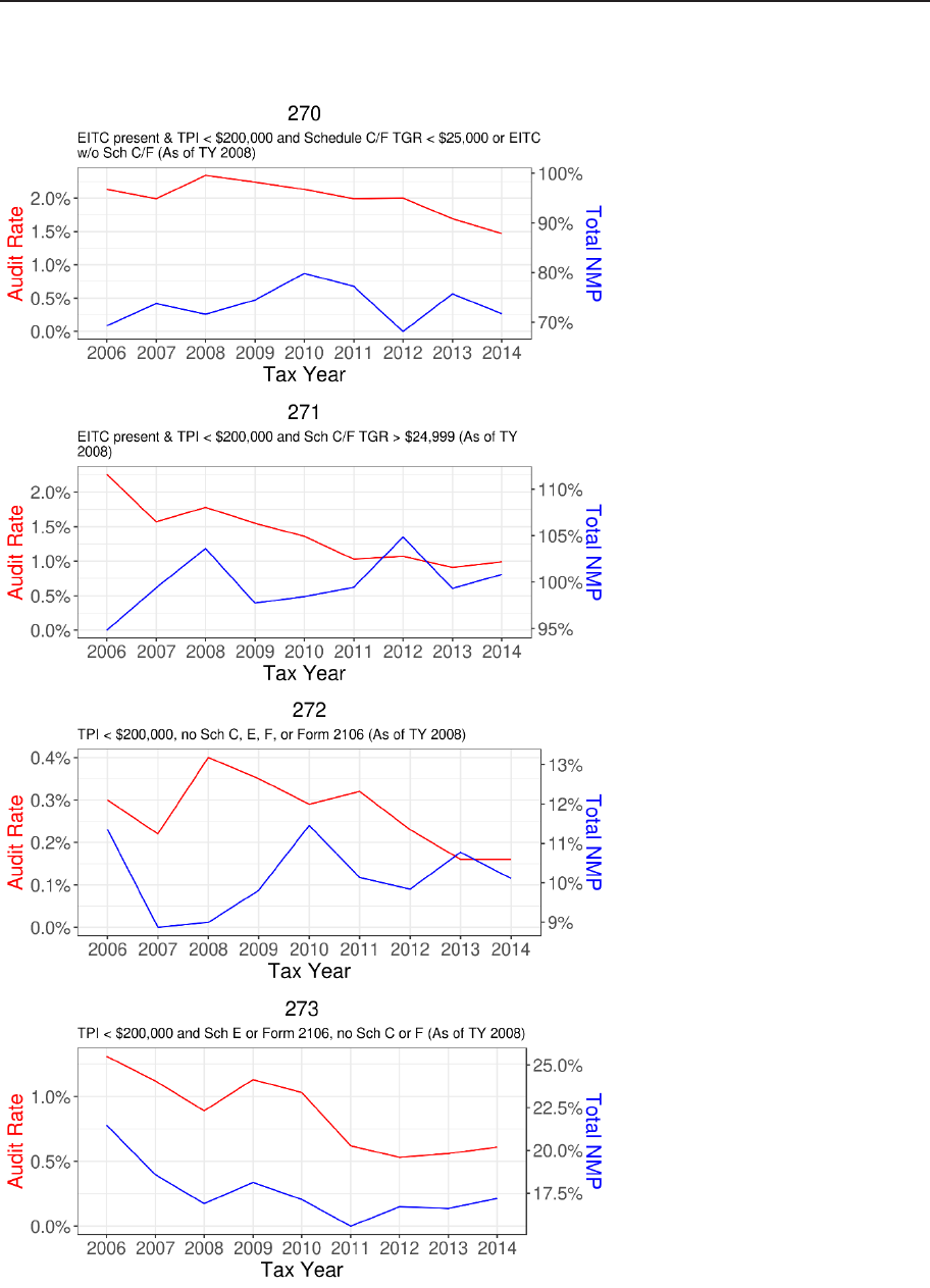
Plumley, Rodriguez, Grana, and McGlothlin
FIGURE 14. Audit Rate vs. Aggregate NMP, by Activity Code (Trimmed Data)

Silver Lining: Estimating the Compliance Response to Declining Audit Coverage
FIGURE 14. Audit Rate vs. Aggregate NMP, by Activity Code (Trimmed Data) (Continued)

Plumley, Rodriguez, Grana, and McGlothlin
FIGURE 14. Audit Rate vs. Aggregate NMP, by Activity Code (Trimmed Data) (Continued)

Silver Lining: Estimating the Compliance Response to Declining Audit Coverage
Supplementary Results
TABLE
Dependent variable: Log NMA
TARC Visibility
Group 1
Visibility
Group 2
Visibility
Group 3
Visibility
Group 4
Visibility
Group 5
Visibility
Group 6
Audit Rate (2-Yr Lag)
0.099*** -0.051
*
** -0.052* -0.119** 0.005 -0.018 -0.149***
(0.025) (0.017) (0.030) (0.051) (0.030) (0.032) (0.024)
Corrected TARC
0.00001***
(0.00000)
Correct Amount for Visibility
Group
-0.00000 0.00000*** 0.00000*** 0.00000*** -0.00000*** -0.00004***
(0.00000) (0.00000) (0.00000) (0.00000) (0.00000) (0.00000)
Total Exemptions 1
1.638*** -0.338*** 0.267** 0.246* 1.707*** 0.658*** 0.651
(0.143) (0.057) (0.114) (0.147) (0.136) (0.089) (0.401)
Total Exemptions 2
3.123*** -0.577*** 0.481*** 0.838*** 1.598*** 3.450*** 1.643***
(0.145) (0.059) (0.118) (0.163) (0.144) (0.092) (0.401)
Total Exemptions 3
3.598*** -0.553*** 0.581*** 1.005*** 1.726*** 3.818*** 2.326***
(0.147) (0.061) (0.121) (0.173) (0.149) (0.096) (0.402)
Total Exemptions 4
3.652*** -0.558*** 0.496*** 0.735*** 1.690*** 3.860*** 2.554***
(0.150) (0.063) (0.124) (0.179) (0.155) (0.101) (0.403)
Total Exemptions 5+
3.995*** -0.473*** 0.546*** 1.188*** 1.882*** 3.996*** 2.987***
(0.153) (0.065) (0.128) (0.187) (0.161) (0.106) (0.404)
Wage Income
-0.092** -0.061* -0.168*** -0.135*** 0.113*** -0.099**
(0.038) (0.032) (0.050) (0.041) (0.042) (0.049)
Claimed child tax credit
-0.229*** -0.057*** -0.193*** -0.038 -0.225*** -0.577*** -0.208***
(0.031) (0.018) (0.034) (0.068) (0.052) (0.034) (0.031)
Itemized
1.386*** -0.300*** 0.056 -0.376*** -0.122** 4.818*** 0.198***
(0.042) (0.027) (0.035) (0.055) (0.058) (0.043) (0.054)
Deducted mortgage interest
-0.477*** -0.048* 0.01 0.382*** 0.398*** -0.723*** -0.400***
(0.041) (0.026) (0.034) (0.056) (0.058) (0.044) (0.053)
Over 65
-0.612*** -0.274*** 0.878*** -0.166*** -0.462*** -0.302*** -0.522***
(0.040) (0.028) (0.032) (0.052) (0.049) (0.043) (0.055)
Used paid preparer
0.033 -0.044*** -0.154*** -0.110*** 0.101*** -0.116*** 0.018
(0.023) (0.013) (0.022) (0.043) (0.037) (0.024) (0.026)
Filed electronically
-0.142*** 0.037** -0.090*** -0.079** -0.286*** -0.065** 0.009
(0.025) (0.015) (0.023) (0.040) (0.035) (0.027) (0.029)
Married-Joint Status
-1.689*** 0.081*** 0.038 -0.422*** 0.176*** -2.763*** -1.046***
(0.033) (0.019) (0.036) (0.080) (0.055) (0.036) (0.035)
Constant
1.264*** 1.298*** 0.818*** 3.083*** 3.235*** 0.166 1.351***
(0.157) (0.067) (0.135) (0.206) (0.160) (0.117) (0.405)
Observations
88,521 72,938 63,795 40,112 58,919 73,990 48,083
Tax Year Fixed eect N N N N N N N
Adjusted R2
0.133 0.022 0.033 0.084 0.235 0.341 0.151
F Statistic
520.980*** 67.154*** 85.658*** 142.824*** 697.565*** 1,473.283*** 329.790***
Degrees of Freedom
88,445 72,854 63,750 40,072 58,864 73,879 48,031
Notes: Standard errors displayed in parentheses. *p<0.10, **p<0.05, ***p<0.01 Corrected amounts (for TARC and by visibility group) are specied in unscaled dollar
values. Although statistically signicant, the estimated coecients are small because the amount of noncompliance is small relative to the overall amount of income or
osets.

3
∇
Understanding Contemporary Taxpayers
Lin ♦ Samarakoon
Lopez-Luzuriaga ♦ Scartascini
Hoopes ♦ Menzer ♦ Wilde

Who Are Married-Filing-Separately Filers
and Why Should We Care?
Emily Y. Lin and Navodhya Samarakoon (Oce of Tax Analysis, U.S. Department of Treasury)
1
1. Introduction
e U.S. federal income tax system recognizes families as an economic unit. Married couples le the income
tax return jointly by pooling the spouses’ incomes and deducting combined allowable expenses. Married cou-
ples can also elect to le separate returns, claiming the Married-Filing-Separately (MFS) ling status, but they
are likely to face a higher tax liability as a result due to the unfavorable tax treatment of MFS status relative to
Married-Filing-Jointly (MFJ) status. Of the . million federal individual income tax returns led for Tax
Year (TY) , . million were led as MFJ and . million were led as MFS.
Counting each MFJ return
as two married lers, for TY , .% of married lers who claimed either ling status led jointly, leaving
only .% electing to le as MFS.
While it is well known that claiming the MFS status generally results in a higher federal income tax li-
ability than claiming the MFJ status, it is little known to what extent married couples who le as MFS have a
separate ling penalty where they face a higher federal income tax liability by ling separately.
Because there
is no single condition or formula to apply, a married couple may not know which ling status leads to a lower
tax liability until they run the calculation for both statuses. e Internal Revenue Service (IRS) Publication ,
Dependents, Standard Deduction, and Filing Information, informs married lers that the combined tax on
separate returns is “generally” higher than the tax they would face on a joint return. e publication instructs
married lers to “gure your tax both ways (on a joint return and on separate returns)” to be certain that they
are “using the ling status that results in the lowest combined tax.”
In addition to a possible lower tax bill,
married couples may le separate returns for non-tax reasons. Numerous online articles, posted mostly by the
media and tax preparation professionals or soware companies, guide married taxpayers on how to choose the
“better’ ling status or when it makes sense to le separately.
In this paper, we summarize the situations in which married couples may prefer to le as MFS and situ-
ations in which ling a joint return may not be a choice for some married individuals. In addition, this paper
lls the knowledge gap by providing novel statistics and data analysis about MFS claims. Possibly because of
the assorted reasons why married couples le as MFS, no single prole can describe the small number of MFS
lers. Our analysis shows that MFS lers consist of a diverse group of taxpayers across the income distribution
and by how long they use this ling status. MFS lers are represented in all segments of the income distribu-
tion, with one-third having Adjusted Gross Income (AGI) below , and % having AGI above ,
in . In addition, using administrative tax data for TYs –, we nd that over the -year period,
more than half of the MFS lers claimed the status for only year, and nearly % used it for years or shorter.
However, about % of those who ever claimed the status during this period did so for more than years.
Examining the extent and the level of the separate ling penalty where a married couple pays more federal
income tax by ling separate returns, our analysis shows that approximately –% of MFS lers have federal
income tax benets by ling separately for an average amount of , (in dollars). Slightly fewer than a
1
e authors would like to thank Adam Cole and the participants in the 2023 IRS/TPC Joint Research Conference for helpful feedback. e authors analyzing the
tax data were employees at the U.S. Department of the Treasury. e ndings, interpretations, and conclusions expressed in this paper are entirely those of the
authors, and do not necessarily reect the views or the ocial positions of the U.S. Department of the Treasury. Any taxpayer data used in this research was kept
in a secured Treasury or IRS data repository, and all results have been reviewed to ensure that no condential information is disclosed.
2
Refer to the Statistics of Income tax statistics posted on https://www.irs.gov/statistics/soi-tax-stats-individual-statistical-tables-by-ling-status.
3
is paper examines only the federal income tax. Examination of the total federal and state liability is beyond the scope of this paper.
4
See page 7 of IRS Publication 501, Dependents, Standard Deduction, and Filing Information

Lin and Samarakoon
quarter of MFS les face the same federal income tax liability when ling a joint return, and about to %
of MFS lers have a federal income tax penalty by ling separately with an average penalty of , to ,.
Taxpayer income and the presence of itemized deductions are positively associated with the bonus status. In
addition, because MFS lers are generally ineligible for the Earned Income Tax Credit (EITC), the separate
ling penalty is more prevalent among MFS lers who would claim the EITC when ling a joint return.
Although MFS status concerns only a small number of taxpayers, this ling status is associated with sev-
eral policy and tax administration issues, including complexity, equity, and compliance. Complexity arises not
only because married couples may have to calculate tax twice to decide on the ling status, but for taxpayers
going through a separation or divorce, it can be confusing to determine the correct ling status. Separating
individuals may have the living arrangements akin to those of unmarried individuals who le as single or
head-of-household, but the tax rules governing marital status for the determination of ling status can be
complicated to understand and interpret. On equity, MFS lers face an unfavorable tax treatment with respect
to refundable tax credits. For low-income individuals who have diculties in ling a joint return with their
spouses, they would be denied the credits by ling as MFS. Lastly, the disparate tax liabilities across ling sta-
tuses, wherein ling as MFS leads to a higher tax liability than ling as unmarried lers, creates an incentive
for separating individuals to misreport ling status. Because there is no third-party information about taxpay-
ers’ ling status, it is challenging for the IRS to detect this potential noncompliance absent an audit.
Our analysis shows that the regulatory and legislative eorts to allow vulnerable MFS lers to claim the
Premium Tax Credit (PTC) and EITC in limited situations resulted in a very small fraction of MFS lers
claiming each credit. Fewer than % of MFS lers claimed the PTC in recent years and, in , the rst year
in which EITC was extended to MFS lers, % of MFS lers claimed the EITC. Because it is dicult to assess
taxpayer eligibility under the specied rules that entitle MFS lers to these credits, further study is needed to
determine whether the current claims are at their potential levels. Also, given the narrowly dened situations
in which these credits are made available for MFS lers, MFS lers may need assistance in understanding their
eligibility.
Finally, using audit results from a stratied random sample of individual income tax returns, we nd that
MFS status is susceptible to misreporting. During TYs –, an average of .% of returns were led
as MFS each year, but the audit results suggest that .% of returns should have used this ling status. e
vast majority of these misreporting cases involved erroneous claims of single or head-of-household status by
audit-determined MFS lers. However, a small percentage of taxpayers incorrectly claimed the MFS status and
as determined by the audit examiner, should pay a lower tax than the amount they reported on the tax return.
II. Tax Rules for Married-Filing-Separately
Prior to the enactment of joint taxation for married couples in , the U.S. income tax system had only one
ling status applied to all individuals regardless of marital status. With the creation of joint taxation in ,
the joint status was used by married individuals, and the single status was used by unmarried individuals,
as well as by married individuals who elected to le separate returns. At that time, the tax bracket schedules
were designed in a way that all married couples paid no more federal income tax by ling jointly than they
would if they led separate returns using the single status. at is, there were federal income tax benets, but
no tax penalties, for married couples to le joint returns. Subsequent tax cuts were extended to unmarried
individuals, which resulted in the marriage penalty and led to disparate tax schedules applied to dierent
groups of non-joint lers. Specically, head-of-household status was created in and expanded in
to reduce the tax burden on unmarried individuals who had family responsibilities; the bracket widths for
unmarried individuals who did not qualify as heads of households were broadened by the Tax Reform Act of
(TRA). In contrast, the tax schedule for married individuals who led separate returns was maintained
in these legislations.
As a result of the TRA, married taxpayers who led separate returns faced a dierent tax schedule from
that for single taxpayers, eective in TY . In addition, not only was MFS status less favorable than MFJ
and head-of-household statuses, but it was also less favorable than single status. Despite frequent tax changes

Who Are Married-Filing-Separately Filers and Why Should We Care?
aer , the bracket disadvantage associated with the MFS status has never been eliminated. Table A- in the
Appendix shows the tax brackets by ling status for TY .
A taxpayer’s marital status for tax ling purposes is determined by the taxpayer’s status on the last day of
the tax year.
A person is considered not married if the person is legally separated from the spouse, accord-
ing to the state law, under a nal decree of divorce or separate maintenance. A married couple can elect to
le a joint return using the MFJ status or separate returns using the MFS status. In addition, certain married
individuals who live apart from their spouses are considered as unmarried for ling status under the so-called
abandoned spouse rules. e abandoned spouse rules are met if the taxpayer furnishes over half of the cost of
maintaining the household that constitutes the principal place of abode of the taxpayer and a qualifying child
for more than half of the tax year, and the taxpayer’s spouse is not a member of the household during the last
months of the tax year. Figure displays a ow chart on the determination of marital status for tax purposes
and the ling status for married taxpayers.
FIGURE 1. Determination of Marital Status and Applicable Filing Status
a
Per the Internal Revenue Code (IRC) Section 7703(a), an individual legally separated from the spouse, according to the state law, under a decree of divorce or of sepa-
rate maintenance, is not considered married for tax purposes.
b
Per IRC Section 7703(b), a married individual meets the abandoned spouse requirements, and thus is considered as unmarried for ling status, if (i) the taxpayer main-
tains as his home a household which constitutes for more than one-half of the tax year the principal place of abode of a qualifying child, (ii) the taxpayer furnishes over half
of the cost of maintaining the household during the relevant taxable year, and (iii) the taxpayer’s spouse is not a member of the household during the last six months of the
taxable year.
As the tax system became more complex, an increasing number of provisions contributed to the unfavor-
able tax outcome for the MFS status relative to other ling statuses. MFS lers face limited eligibility for tax
credits. ey were not eligible for the EITC until TY 2021 when limited exceptions were allowed. ey have
very limited eligibility for the PTC and the Child and Dependent Care Tax Credit (CDCTC). ey cannot take
the education credits and the adoption tax credit at all, and are eligible for a reduced amount of the saver’s
credit. In addition to the unfavorable treatment with respect to tax credits, other rules lead to a higher tax li-
ability for MFS status.
6
Specically, MFS lers cannot take the exclusion for adoption expenses, the deduction
for student loan interest, or the exclusion for interest income from qualied U.S. savings bonds used for higher
education expenses. e maximum amount of the child and dependent care exclusion is half the size for MFS
lers than for other taxpayers. If one spouse claims itemized deductions on the MFS return, the other spouse
cannot take the standard deduction. In certain situations, MFS lers cannot claim the credit for the elderly
or the disabled and must include in income a higher percentage of Social Security benets. In addition, the
income range of the phase-out schedule for the save’s credit, the Child Tax Credit (CTC) and the credit for
other dependents (ODC), as well as the exemption level for the Alternative Minimum Tax and the capital loss
5
If a spouse dies during a tax year, the determination is made as of the time of the death.
6
Refer to IRS Publication 501.

Lin and Samarakoon
deduction limit are lower for MFS status than for MFJ status. ese tax features could further increase the tax
liability associated with MFS status for some married couples.
MFS lers are eligible to claim the PTC,
7
EITC,
8
and CDCTC
9
in limited circumstances. In March 2014,
the IRS extended eligibility for the PTC to victims of domestic abuse and spousal abandonment, but a taxpayer
cannot claim this relief for more than 3 consecutive tax years. To be eligible, the taxpayer must live apart from
the spouse at the time of ling the tax return. A taxpayer is a victim of spousal abandonment if they cannot
locate the spouse aer a reasonably diligent eort is made (Mitchell (2016)). Beginning in 2021, separating
couples who le as MFS may claim the EITC if they are separated under a legally binding, written separation
agreement (but not a decree of divorce) and live apart from their spouses at the end of the tax year, in addition
to meeting the same eligibility rules as the EITC. MFS lers may also be eligible to claim the EITC if they meet
the abandoned spouse rules except for the household maintenance test. As for the CDCTC, MFS lers may be
eligible to claim the credit if they meet the abandoned spouse rules except that the household they maintain is
the home they reside in with a qualifying person for the CDCTC purposes (e.g., a disabled sibling) who is not
a dependent child.
10
Table 1 summarizes the credit eligibility rules for MFS lers, most of which are similar to
the criteria for being considered as unmarried for ling status.
For some married taxpayers, electing MFS status may result in a lower tax liability than ling jointly. If one
spouse has low income and signicant deductions subject to an AGI oor, it is possible that ling separately
is advantageous. For example, medical expenses are deductible to the extent that expenses exceed 7.5% of a
taxpayer’s AGI. In the same manner, prior to 2018, business, investment, and certain miscellaneous expenses
were deductible, subject to a 2% AGI oor. In a dierent scenario, if either spouse is a nonresident alien at
any time during the tax year, the couple cannot le as MFJ and each spouse generally uses MFS status to re-
port income subject to U.S. tax. However, U.S. persons married to a nonresident alien may elect to treat the
nonresident alien spouse as a resident alien and le a joint federal income tax return. With this election, the
worldwide income of both spouses is subject to U.S. income taxation, which can lead to undesirable tax con-
sequences (Drumbl (2016)). Finally, based on the laws and regulations at the state level, the ling status choice
on the federal return(s) may inform or determine the ling status the spouses may use on the state return(s).
e ling status that minimizes the federal income tax liability may not be the same status that minimizes the
total federal and state income tax liability. is paper focuses on the federal tax liability and leaves the choice
of ling status when state tax is considered for future research.
7
Refer to IRS Publication 974.
8
Refer to IRS Publication 596.
9
Refer to IRS Publication 503.
10

Who Are Married-Filing-Separately Filers and Why Should We Care?
TABLE 1. Criteria for MFS Filers To Qualify for Tax Credits
Criteria or variations
Criterion for a
married
individual to
of-household
When electing MFS status, is the criterion necessary to qualify for…
CDCTC
EITC: either (1) or (2)
PTC
(1) (2)
Furnishes over half of the
cost of maintaining the
household during the rel-
evant taxable year
Yes Yes
Maintains as the taxpayer’s
own home a household
which constitutes the prin-
cipal place of abode for a
qualifying child for more than
one-half of the tax year
Yes
Maintains as the tax-
payer’s own home
a household which
constitutes the prin-
cipal place of abode
for a qualifying
CDCTC person for
more than one-half
of the tax year
Yes Yes
The taxpayer’s spouse is not
a member of the household
during the last 6 months of
the taxable year
Yes Yes Yes
Spouse does not
live in the same
household at the
end of the taxable
year
Spouse does
not live in the
same household
at the time of tax
ling
Taxpayer and spouse are
separated under a legally
binding written separation
agreement or a decree of
separate maintenance
Yes
Is unable to le jointly be-
cause the taxpayer is a vic-
tim of domestic abuse or is
unable to locate the spouse
after reasonable diligence
Yes
Note
All of the above
are met
All of the above and
CDCTC eligibility
are met
All of the
above and
EITC eligibil-
ity are met
All of the above
and EITC eligibil-
ity are met
All of the above
and PTC eligibil-
ity are met;
cannot use the
relief for more
than 3 consecu-
tive years
Data source: Author tabulation of tax rules and instructions in IRS publications.
III. Possible Non-Tax Reasons To Claim Married-Filing-Separately Status
Some married taxpayers may le as MFS involuntarily. Treasury regulations, as outlined above, allow domestic
abuse and spousal abandonment exceptions for MFS lers to claim the PTC. In the instance of spousal abuse,
the perpetrator may be noncooperative, refusing to furnish the necessary nancial information needed to le
jointly. It is also possible that the victim has le the home and does not wish to contact the abuser to le a
joint return. For spousal abandonment, if the taxpayer does not have dependent children, does not meet the
household maintenance test, or does not live apart from the spouse for the last six months of the tax year, the

Lin and Samarakoon
taxpayer is considered married and, because the spouse cannot be located, the taxpayer would have no choice
but to le as MFS. With the PTC exception, the taxpayer may take the credit.
Married couples may le separately if each spouse would like to be responsible only for their own tax
liability. In general, when a joint return is led, both spouses are responsible for the tax and interest or penal-
ties due on the return except for limited situations. Married taxpayers may le separately if they distrust that
the spouse is accurately reporting the nancial situation for tax purposes. In these cases, electing MFS status
protects a taxpayer from IRS audits conducted on the spouse’s tax return. Along a similar vein, choosing MFS
status could protect a married person from being liable for the spouse’s tax bill or from a refund oset that
applies to the spouse. Estranged spouses who no longer live together or who do not have an emotionally co-
dependent relationship may not share nancial information to le a joint return. Couples in the process of get-
ting a divorce may le separately to avoid the potential hassle of dealing with the IRS on a joint return aer the
divorce. It is not uncommon for couples in the process of a divorce to le separate returns. ese individuals
may use MFS status if they are not legally separated under a required court action or do not meet the specied
rules such as living apart for the last months of the year. Finally, married couples may le separately simply
because the spouses want to stay nancially independent.
One scenario in which it may be nancially benecial for married couples to le separate returns is if a
taxpayer has large student loan expenses subject to an income-based repayment plan (Drumbl ()). When
married taxpayers le jointly, the repayment amount will be based on the spouses’ total incomes and therefore
may be higher than if they le the tax separately. Lastly, married taxpayers may simply, and unfortunately, le
separately because they lack access to necessary and accurate tax advice on what ling status would provide
the most benecial tax outcome.
IV. Data Analysis
A. Shares of MFS Returns and Income Distribution
Table presents the shares of returns by ling status. Between TYs and , the percentage of MFS re-
turns grew steadily from .% to .% of total returns each year. MFS lers, along with single lers, have made
up a rising share of the tax-ling population over the past decade. Conversely, the shares of MFJ and head-
of-household lers have declined. us, MFS returns, despite constituting a small fraction of all returns, have
increased in relative and absolute terms. Counting each MFJ return as two married lers, the share of married
lers used MFS status increased from .% to .% during the period. Because some separate-ling spouses
claimed head-of-household status, including these individuals resulted in .% of married lers ling separate
returns for TY .
TABLE 2. Shares of Returns by Filing Status, 2011-2020
Tax Year
Number of All
Returns
Married-Filing-
Jointly
Married-Filing-
Separately
Head-of-
Household
Single
Share of
Married Filers
Using MFS
2011 145,370,240 36.7% 1.8% 15.2% 46.3% 2.4%
2012 144,928,471 37.1% 1.8% 15.1% 46.0% 2.4%
2013 147,351,298 36.6% 1.9% 14.9% 46.5% 2.5%
2014 148,606,578 36.3% 2.0% 14.9% 46.8% 2.7%
2015 150,493,262 36.1% 2.0% 14.7% 47.2% 2.7%
2016 150,272,156 36.0% 2.0% 14.4% 47.5% 2.7%
2017 152,903,232 35.8% 2.1% 14.3% 47.8% 2.9%
2018 153,774,296 35.7% 2.1% 14.2% 48.0% 2.9%
2019 157,796,805 34.7% 2.4% 13.7% 49.2% 3.3%
2020 164,358,794 33.7% 2.4% 13.1% 50.9% 3.4%
Data Source: Author calculations from data published in IRS SOI Publication 1304, Individual Income Tax Returns Complete Report (years 2011 through 2020).

Who Are Married-Filing-Separately Filers and Why Should We Care?
By TY , . million taxpayers led as MFS. Table breaks down the returns by AGI for each ling
status in TY , the most recent year for which the IRS’s published statistics are available (IRS ()). MFS
lers were represented in all income segments, but the fractions were higher than average for the income range
of , to ,. Compared with other ling statuses, the income distribution suggests that MFS lers
had higher income relative to single and head-of-household lers. In addition, when the spouses’ incomes on
separate returns were added to arrive at couple-level income, Table shows that separate-ling couples were
more likely to have income below ,, and less likely to have income of , or more, compared to
joint-ling couples.
TABLE 3. Distribution of Income by Filing Status for TY 2020
Adjusted
Gross Income
(AGI, $)
All Returns
Married-
Filing-Jointly
Married-
Filing-
Separately
Head-of-
Household
Single
Couples Filing
Separately
≤ 0 3.2% 1.7% 4.0% 1.2% 4.7% 3.0%
0–15k 18.9% 5.2% 13.1% 14.8% 29.2% 6.8%
15k–30k 17.8% 7.6% 15.1% 29.2% 21.7% 8.2%
30k–50k 18.2% 11.5% 24.7% 27.9% 19.8% 13.4%
50k–75k 13.8% 14.7% 20.1% 14.4% 12.7% 18.0%
75k–100k 8.7% 14.7% 9.2% 6.1% 5.5% 15.0%
100k–200k 13.6% 30.2% 11.2% 5.2% 5.0% 26.0%
200k–500k 4.6% 11.5% 1.8% 1.0% 1.1% 8.2%
500k–1 million 0.8% 1.9% 0.4% 0.1% 0.2% 0.8%
≥1 million 0.4% 0.9% 0.3% 0.1% 0.1% 0.6%
Total 100.0% 100.0% 100.0% 100.0% 100.0% 100.0%
Count 164,358,792 55,322,922 3,919,416 21,463,538 83,652,916 2,026,869
Data Source: Author calculation of the IRS Statistics of Income publications (IRS (2020)) and individual income tax returns led for TY 2020.
a
Of all MFS returns led for TY 2020, 2.45 million returns can be paired, based on the taxpayer’s and the spouse’s identication numbers provided on the returns, as
being led by 1.22 married couples. Approximately 0.26 million MFS lers had a spouse who claimed the head-of-household status, and another 0.54 million MFS lers
had a spouse who did not le a tax return, who we assumed had no income. The total includes 2.02 million married couples where at least one spouse led as MFS.
Couple-level income cannot be calculated for MFS lers who did not provide information about the spouse’s taxpayer identication number. These lers are not included
in this column.
B. Tax Penalty for Filing Separately
One way to assess the reasons why married couples le separately is to understand the prevalence and the level
of tax penalty and bonus faced by MFS couples. e source of data we use for this evaluation is the population
of approximately . million MFS returns led for TYs to . When a married couple les separately,
the two MFS returns could be paired and the potential tax liability of the couple led jointly can be calcu-
lated and compared with the combined liability on the separate returns. MFS lers are instructed to enter the
spouse’s name and either the Social Security Number (SSN) or Individual Taxpayer Identication Number
(ITIN) on the tax return. We link an MFS return to the spouse’s MFS return where the spouse’s identication
number matches the ler’s identication number on another MFS return. is link results in . million mar-
ried couples where both spouses claimed the MFS status for a total of . million MFS returns in the data.
A large number, about 13.2 million, of MFS returns in our le are not linked to another MFS return for the
spouse for various reasons. First, about 2.2 million MFS lers had a spouse who claimed the head-of-house-
hold status. For the analysis, we use the information reported on the spouses’ head-of-household returns to
calculate the couples’ tax liability if ling jointly. Next, 2.1 million 1040-NR returns were led by nonresident
aliens who did not provide the spouse’s Taxpayer Identication Number (TIN), either the SSN or ITIN. We
11
the Social Security Number or Individual Taxpayer Identication Number
the spouse-matching results.

Lin and Samarakoon
assume the spouse was also a nonresident alien and exclude these 1040-NR MFS returns from analysis because
these couples cannot use MFJ status. In addition, we exclude another 4.4 million MFS returns for which the
spouse’s TIN was missing or the spouse’s TIN was found on a joint return for the same tax year because it is
not straightforward as to how to determine these spouses’ tax liability when ling as MFS.
12
For the rest of the
4.5 million unmatched returns, for which the spouse’s identication number was available and did not appear
on any tax return for the same tax year, the analysis assumes that these spouses were nonlers and did not
have income. We present results including and excluding these nonler cases. Also, Table A-2 in the Appendix
shows the counts and percentages of the MFS returns with the various matching outcomes.
We use the TAXSIM model (Feenberg and Coutts (1993)) to simulate a couple’s federal tax liability when
the couple les jointly as well as the spouses’ combined federal tax liability when ling separately.
13
We then
take the dierence between the two simulated liabilities (in 2021 dollars) to calculate the tax penalty (in nega-
tive values) and bonus (in positive values) facing the couple when the spouses le separate returns. We use a
threshold of $5 to dene the separate ling penalty or bonus. at is, a couple is considered as having a sepa-
rate ling penalty (bonus) when the combined liability on the two separate returns is higher (lower) than the
liability on the joint return by more than $5. e evaluation of the penalty or bonus is at the couple level, and
the outcome for a couple applies to both spouses in the matched cases.
Table 4 presents the simulation results for all MFS returns as well as for MFS returns where both spouses
led a return. e average separate ling penalty is $646 for matched MFS returns and $987 for all MFS
returns, including nonler cases. Most MFS lers face a separate ling penalty; about 53% of matched MFS
lers and 59% of all MFS lers have a penalty, averaging $1,863 and $2,140, respectively. Slightly fewer than a
quarter of MFS lers face the same liability ling separately or jointly, whereas about 19% to 23% have a bonus
by ling separately, with a bonus amount of $1,513 on average. To put the amount of penalty and bonus in
context, the total separate ling penalty represents about 12% (for matched returns) or 17% (for all returns) of
the total joint liability for those who face a separate ling penalty. In comparison, the total separate ling bonus
as a ratio of total joint liability is about 9%.
12
Future research may explore ways to incorporate the spouse’s tax information for the 3.2 million MFS returns with a missing spouse TIN through returns led in
dierent years.
13
For this paper, we use TAXSIM version 32.

Who Are Married-Filing-Separately Filers and Why Should We Care?
TABLE 4. Mean Variables of Tax Simulation Results for MFS Returns
Variable ALL
Separate Filing
Penalty
Neutral
Separate Filing
Bonus
All MFS Returns, Including Couples Where One Spouse Did Not File
Tax penalty ($)
a
-987 -2,140 0 1,513
Fraction of all returns 100% 59.35% 21.93% 18.72%
Penalty as % of joint liability
b
-7.45% -17.34% 0% 9.15%
Adjusted gross income ($) 58,244 58,456 49,727 67,553
Age 46.96 47.51 45.99 46.37
Itemizer (0/1), self or spouse 0.3351 0.2902 0.1699 0.6713
Child tax credit (0/1) 0.1698 0.1786 0.1364 0.1811
EITC on joint return (0/1) 0.1041 0.1560 0.0054 0.0552
CDCTC on joint return (0/1) 0.0267 0.0236 0.0005 0.0673
Number of dependents 0.3251 0.3493 0.2454 0.3417
Any dependents (0/1) 0.2136 0.2235 0.1732 0.2295
Number of observations 24,761,774 14,695,734 5,431,231 4,634,809
Fraction with penalty or bonus by spouse ling status:
Spouse MFS 100% 56.73% 26.78% 16.49%
Spouse head-of-household 100% 24.01% 2.22% 73.76%
Spouse nonler 100% 88.11% 11.89% 0%
Matched MFS Returns Only
Tax penalty ($)
a
-646 -1,863 0 1,513
Fraction of all returns 100% 53.16% 24.09% 22.75%
Penalty as percent of joint liability
b
-4.13% -11.77% 0% 9.15%
Adjusted gross income ($) 61,533 61,523 55,871 67,553
Age 46.62 47.44 45.03 46.37
Itemizer (0/1), self or spouse 0.3636 0.3180 0.1736 0.6713
Child tax credit (0/1) 0.1610 0.1602 0.1439 0.1811
EITC on joint return (0/1) 0.0630 0.0924 0.0054 0.0552
CDCTC on joint return (0/1) 0.0325 0.0320 0.0005 0.0673
Number of dependents 0.2969 0.3033 0.2406 0.3417
Any dependents (0/1) 0.2020 0.2025 0.1750 0.2295
Number of observations 20,376,065 10,831,696 4,909,576 4,634,793
Data source: Individual income tax returns led for TYs 2013–2021.
Notes: The data contain 31,805,626 MFS returns. A total of 6,508,7554 returns are excluded from the analysis either because both spouses are nonresident aliens or the
spouse’s tax liability is not readily determinable. Another 99 observations are dropped in simulation due to missing variables. The table also excludes 543,998 returns
(or 2.1% of returns in simulation) for which the dierence between the simulated federal tax and the reported tax for either spouse is greater than $15,000, following an
approach in Lin and Tong (2017). All money amounts are in 2021 dollars.
a The tax penalty evaluated at the couple level is applied to the spouse(s).
b This is the ratio of total penalty to total tax.
Table 4 shows that MFS lers in tax-neutral status have the lowest income of the three groups of MFS lers
by penalty status. Low-income taxpayers may have no tax liability under either ling status and, thereby do not
incur either the penalty or bonus. In addition, given the tax-related reasons for ling separately, as expected,
claiming itemized deductions is positively related to having tax savings by ling separate returns. Nearly 70%
of those with a bonus itemized their deductions, compared to the average rate of 35% for all MFS lers. Not
reported in the paper, the bonus rate dropped by 40% in TY 2018 aer the enactment of tax changes in the Tax
Cuts and Jobs Act (TCJA) that signicantly lowered the fraction of taxpayers who beneted from itemizing

Lin and Samarakoon
deductions. Specically, for MFS lers matched to the spouses’ returns, the share with the bonus declined from
28% before 2018 to 17% in 2018, and the share with the bonus for all MFS lers, including those with nonl-
ing spouses, declined from 23% to 14%. Another variable that is positively associated with the bonus status is
taxpayer income, which may be related to the presence of itemized deductions.
In contrast, the separate ling penalty is more prevalent among individuals who would receive the EITC
when they led jointly. Because MFS lers generally cannot claim the credit, claiming it when ling a joint
return would result in the separate ling penalty. About 16% (9%) of all (matched) MFS lers with the separate
ling penalty would receive the EITC when ling jointly, exceeding the average rate of 10% (6%). For the same
reason, the bonus rate was high, and the penalty rate was low, for MFS lers whose spouses led as head-of-
household because the head-of-household spouses could claim the EITC on their own returns. e bottom
three rows of the top panel show the penalty percentages by the spouse’s ling status. Only 24% of MFS lers
with a head-of-household spouse incur the separate ling penalty, compared to 59% of all MFS lers.
C. Longitudinal Data on the Use of MFS Status
No data are available to accurately group MFS lers by reason for electing this status. We hypothesize that the
duration for which an individual uses this ling status may inform the possible reason. In many of the sce-
narios as laid out above, the situation, such as if the couple is going through a divorce or if a separating couple
misses the -month test in the rst taxable year, but continues to live apart in future years, may be temporary.
Hence, couples with shorter MFS election periods may be in transition from being married to single or have
temporary diculties in ling jointly. A long duration of MFS claims may indicate a prolonged separation with
neither spouse meeting the abandoned spouse rules or any longer-term scenarios such as when spouses would
like to keep tax or nancial independence. Persistent MFS elections may also suggest a tax bonus from ling
separate returns. Understanding the distribution of the length of MFS claims also helps to assess the extent
to which a policy or tax law change aecting this ling status would have a short-term or long-term eect on
taxpayers.
During the 9-year period from 2013–2021, about 13.4 million individuals with unique TINs claimed the
MFS status for a total of 31.8 million tax returns. Calculating the number of years for which an individual used
this ling status, we nd that the majority of individuals who ever claimed the MFS status used it for a relative-
ly short period a time. Table 5 shows that more than half of the individuals claimed the status for only 1 year,
and nearly 80% used it for 3 years or shorter. However, about 5% of those who ever claimed the status did so for
more than 7 years. On average, long-term users of MFS status are older and have a higher income compared
to short-term users, with the average age and AGI increasing with the number of years for ling separately.

Who Are Married-Filing-Separately Filers and Why Should We Care?
TABLE 5. Characteristics and the Percentages of Taxpayers by Duration of MFS Claims in
2013–2021
Number of Years
with MFS Filing
Percentage of All
MFS Filers
Accumulated
Percentage
Mean Age in 2021
Mean Adjusted
Gross Income (AGI)
in 2021$
1 51.7% 51.7% 46 $55,290
2 18.3% 70.0% 48 $59,228
3 9.8% 79.8% 49 $64,292
4 6.0% 85.8% 51 $65,794
5 4.1% 89.9% 53 $67,757
6 2.9% 92.8% 54 $73,397
7 2.3% 95.1% 55 $74,360
8 1.9% 97.0% 57 $98,647
9 3.0% 100.0% 61 $118,026
Data source: Individual income tax returns led as MFS for TYs 2013 to 2021.
Notes: Results in this table are calculated based on 13,370,930 individuals who ever led as MFS in 2013–2021. For the mean AGI listed in the last column, we
calculate the average AGI in 2021 dollars of each individual over the years when they led as MFS, and then take the mean of the individual-level average across all
individuals.
V. Complexity, Equity, and Compliance
Determining the ling status can be confusing for couples who are separated or in the process of getting a
divorce. Taxpayers may not know if their separation agreement or living situations meet the standard of being
considered as unmarried for ling status purposes. Under the tax code, separating couples are considered as
unmarried only if they are separated under a court action recognized by state law as permanently severing the
marriage relation. is denition excludes a non-nal decree of divorce, a legally binding written separation
agreement, or a court order of support. Further complicating the situation, due to dierences in state law, the
court action that meets the standard of legal separation varies across states (Ulven ()). As stated above,
the tax code also provides an exception for married couples living apart to be considered as unmarried. e
abandoned spouse rules are determined based on the couple’s living arrangements, but they do not apply to
separating individuals who do not have dependent children, do not live apart from their spouses for a required
period, or do no furnish more than half of the cost of maintaining the household.
ese restricted rules in dening marital status can disadvantage low-income taxpayers going through a
separation or divorce. Low-income taxpayers may lack the resources to obtain tax advice that would help them
minimize tax liability and determine the correct ling status. Consequently, they may be prone to paying a
higher tax by ling separately or using an incorrect ling status inadvertently. In addition, a study nds that
couples in prolonged separation tend to have low family income, have young children, and be racial and ethnic
minorities (Taxpayer Advocate Service (2012)). Couples in extended separation may have no choice but to le
separate returns from their estranged spouses because the spouse cannot be located or refuses to le jointly.
However, they may remain married for a long time for tax ling purposes because they are not legally sepa-
rated under a required court action and do not meet the abandoned spouse rules. For low-income taxpayers,
the requirement to furnish more than half of the cost of maintaining the household can be particularly chal-
lenging as means tested public programs, such as food stamps and rental subsidies, count as outside support.
To a limited extent, this equity concern over vulnerable taxpayers was addressed by allowing certain MFS
lers to claim a tax credit. Given the narrowly dened circumstances in which MFS lers may be eligible for
these credits, as described in Section II, and the similar, but disparate, eligibility rules for each credit, it is
important for low-income MFS lers to receive necessary assistance in understanding their eligibility. Table
6 shows the fractions of MFS lers who received the PTC, EITC and the CDCTC. e PTC was claimed by
0.6%–1.8% of MFS lers each year, with the fractions increasing gradually over the period. About 2% of MFS
lers claimed the EITC in 2021, the rst year in which the credit was extended to MFS lers. A persistent small

Lin and Samarakoon
fraction, less than 1%, of MFS lers claimed the CDCTC each year. With slightly fewer than 4 million taxpay-
ers ling as MFS in recent years, only approximately 40,000 (1% of total) to 80,000 (2% of total) MFS lers
claimed each of these credits. is result suggests that the special rules that relax the credit eligibility for MFS
lers in sympathetic circumstances have created several very small groups of MFS lers claiming various tax
credits. However, whether the current claims represent their potential levels is largely unknown because it is
dicult to assess taxpayer eligibility under these special rules.
TABLE 6. Share of MFS Filers Claiming Certain Tax Credits, 2013–2021
Tax Year PTC EITC CDCTC
b
2013 X X 0.6%
2014 0.6% X 0.5%
2015 1.1% X 0.4%
2016 1.3% X 0.5%
2017 1.4% X 0.5%
2018 1.5% X 0.5%
2019 1.4% X 0.5%
2020 --
a
X 0.4%
2021 1.8% 2.0% 0.9%
Data source: Individual income tax returns led as MFS for TYs 2013–2021.
Notes: The table is calculated based on a total of 31,805,626 MFS returns. “X” indicates that the credit was not available in the year (PTC) or not available for MFS
status (EITC).
a We cannot use the same tax forms to calculate the share of MFS returns claiming the PTC for 2020 due to a temporary change in the requirement to repay excess
advance payments of the PTC for that year.
b For TYs 2013–2020, the share is calculated based on the claims reported on Form 1040. We cannot use the same tax variable for 2021 due to the temporary
expansion of the credit that resulted in changes to the tax form. The reported share for 2021 reects the percentage of returns reporting the child and dependent care
expenses on Form 2441.
According to the IRS, claiming an incorrect ling status is one of the common errors taxpayers make on
their returns.
14
Not only do the complex rules increase the likelihood that taxpayers make inadvertent errors in
ling status, but the lack of third-party information about individuals’ marital status and living arrangements,
coupled with the disparate liabilities across ling statuses, also makes ling status susceptible to intentional
errors. Absent an audit, IRS does not know whether a previously married person has the required court action
for legal separation to be considered as unmarried. In addition, facts and circumstances of married couples
living apart are similar to those of unmarried persons ling as single or head-of-household, especially because
the abandoned spouse rules for married lers resemble the criteria for the head-of-household status for un-
married lers. Using data from random audits from TYs 2006–2008, Leibel (2014) nds that about 4% of all
EITC claimants, including 2% of single taxpayers and 9% of head-of-household taxpayers claiming this credit,
had MFS as the audit-determined ling status and thereby were ineligible for the credit. Hence, although the
special rules that allow MFS lers to claim certain credits add to tax complexity, they may reduce the incentive
for separating couples to misreport ling status as unmarried persons to claim the credits.
We investigate the extent of taxpayer reporting errors associated with MFS status using data from random
audits. Table 7 shows the results from the audits of a stratied random sample of individual income tax returns
conducted by the IRS’s National Research Program (NRP) for TYs 2006–2014. During this period, an average
of 1.74% of tax returns claimed the MFS status each year. However, according to the ling status determined
by the examiner, an average of 2.68% of tax returns should have claimed this ling status. e additional 0.94
percentage points come from 1.02% of returns that should have led as MFS, but erroneously used either
head-of-household (making up 79% of the erroneous claims) or single (the remaining 21% of the erroneous
claims) status. is is net of 0.08% of returns that should have led as MFJ, but erroneously used the MFS
status. Overall, there is a large degree of misreporting associated with MFS status (1.10% of all returns) relative
to the level that should be reported (2.68% of all returns).
14
https://www.irs.gov/newsroom/common-errors-on-a-tax-return-can-lead-to-longer-processing-times).

Who Are Married-Filing-Separately Filers and Why Should We Care?
TABLE 7. Filing Status Errors Associated with MFS Status, 2006–2014
Reported Filing Status
Is MFS
(% of All Returns)
Corrected Filing Status Is MFS (% of All Returns)
No Yes Total
No 97.24 1.02 98.26
Yes 0.08 1.65 1.74
Total 97.32 2.68 100.00
Data source: The NRP 1040 Study, 2006-2014.
Note: Results in this table are calculated based on 126,668 tax returns in the NRP 1040 Study for TYs 2006–2014.
For the total 1.10% of returns that made ling status errors associated with MFS status, we investigate the
tax adjustments recommended by NRP examiners for these returns.
15
Table 8 shows the results by the type
of errors. For returns where the ling status was changed from single or head-of-household to MFS by the
examiner, the vast majority, or 96%, had a positive adjustment, meaning that the audit-corrected liability ex-
ceeded the liability reported on the return. Also, nearly 70% of these returns, as determined by the examiner,
overclaimed the two child-related refundable credits. e audit-recommended increase in tax liability was
$4,196 on average, including a recommended decrease of $2,318 in the two refundable credits. For returns that
were corrected away from MFS status, 60% had a positive tax adjustment, whereas one-third had a negative
adjustment. Refundable credit errors were not prevalent among these returns. e fact that some taxpayers
overreported their liability by claiming the MFS status may indicate taxpayer confusion about their correct
ling status.
TABLE 8. Recommended Tax Adjustments for Returns Associated with MFS Filing Status
Errors
Adjustment Type
Reported Other Status,
Corrected to MFS
Reported MFS, Corrected to
Other Status
Mean Std. dev. Mean Std. dev.
Adjustment for tax after credits ($) 4,196 4,791 2,204 8,046
Positive adjustment (0/1) 0.9619 0.1915 0.5992 0.4924
Negative adjustment (0/1) 0.0139 0.1171 0.3372 0.4750
Adjustment for EITC and additional CTC ($) -2,318 2,497 -106 1,077
Negative adjustment (0/1) 0.6842 0.4651 0.0651 0.2480
Positive adjustment (0/1) 0.0118 0.1081 0.0463 0.2110
Number of observations 937 106
Data source: The NRP 1040 Study, 2006–2014.
Note: All money amounts are in 2021 dollars.
VI. Conclusion
Fewer than million federal individual income tax returns were led as MFS for TY , representing only
.% of all returns or .% of married lers. Because married couples generally face a higher federal income
tax liability by ling separate returns, this paper examines the characteristics of MFS lers to understand why
and how taxpayers use this ling status. We nd that despite constituting a small share of taxpayers, MFS lers
consist of a diverse group of individuals by income and by how long they use this ling status. MFS lers were
represented in all segments of the income distribution and, while most MFS lers used the ling status for a
15
other errors.

Lin and Samarakoon
brief period, a small fraction used it for more than years. is nding is by no means surprising because, as
documented in the paper, married taxpayers in dierent circumstances may le as MFS for a variety of reasons.
Our analysis further shows that most MFS lers incur a separate ling penalty by paying more federal
income tax than they would if they led jointly with their spouses. Only 19%–23% of MFS lers enjoy a fed-
eral income tax bonus by ling separately, slightly fewer than a quarter of MFS lers face the same tax liability
between ling separately and ling jointly, and 53–59% have a separate ling penalty by claiming the MFS
status. e bonus status is positively associated with taxpayer income and the claim of itemized deductions. In
contrast, the separate ling penalty is more prevalent among MFS lers who would receive the EITC if ling
joint returns.
Finally, this paper considers complexity, tax administration, and compliance issues associated with the
MFS status. Complexity arises because, for certain married taxpayers who are separated from the spouses,
their living arrangements may be akin to those of unmarried individuals, but they are not considered as un-
married for tax ling unless very specic criteria are met. Taxpayers who have diculties in ling joint returns
but remain married must le as MFS, which makes them ineligible for various tax credits. Although the credit
eligibility rules were relaxed for vulnerable MFS lers in limited circumstances, the percentage of MFS lers
who claimed these credits was extremely low. Given the restrictive credit eligibility criteria, MFS lers may not
know about their eligibility without IRS outreach and assistance. Finally, due to the tax incentive for separating
persons to le as unmarried and a lack of third-party information for the IRS to verify ling status, compli-
ance with MFS status is a concern. Our analysis shows a large percentage of ling status errors are associated
with MFS status, some of which likely results from taxpayer misunderstanding about the correct ling status.

Who Are Married-Filing-Separately Filers and Why Should We Care?
References
Drumbl, Michelle Lyon. (2016). “Joint Winners, Separate Losers: Proposals to Ease the Sting for Married
Taxpayers Filing Separately.” Florida Tax Review, 19(7): 399–464.
Feenberg, Daniel and Elisabeth Coutts. (1993). “An Introduction to the TAXSIM Model.” Journal of Policy
Analysis and Management, 12(1), 189–194.
IRS. various years. SOI Tax Stats—Individual Income Tax Returns Complete Report. Publication 1304. https://
www.irs.gov/statistics/soi-tax-stats-individual-income-tax-returns-complete-report-publication-1304.
Leibel, Kara. (2014). “Taxpayer Compliance and Sources of Error for the Earned Income Tax Credit Claimed
on 2006–2008 Returns.” IRS Publication 5161. https://www.irs.gov/pub/irs-soi/15rpeitctaxpayercomplianc
etechpaper.pdf.
Lin, Emily Y. and Patricia K. Tong. (2017). “Using Administrative Tax Data to Estimate Work Participation
and Earnings Elasticities of Married Couples.” International Tax and Public Finance, 24(6), 997–1025.
Mitchell, David S. (2016). “An Unhappy Union: Married Taxpayers Filing Separately and the Aordable Care
Act’s Premium Tax Credit.” Tax Lawyer, 69(2): 453–476.
Taxpayer Advocate Service. (2012). “National Taxpayer Advocate 2012 Annual Report to Congress.”
Ulven, Mark. (1992). “e Separation Penalty: Problems in Establishing Legal Separation for Filing Status.”
Tax Lawyer, 45(3): 903–913.

Lin and Samarakoon
Appendix
TABLE A-1. Tax Brackets by Filing Status, TY 2022
2022 Individual Income Tax Table
Marginal Tax
Rate
Taxable Income
Married-Filing-Jointly
Married-Filing-
Separately
Head-of-
Household
Single
over not over over not over over not over over not over
10% $0 $20,550 $0 $10,275 $0 $14,650 $0 $10,275
12% $20,550 $83,550 $10,275 $41,775 $14,650 $55,900 $10,275 $41,775
22% $83,550 $178,150 $41,775 $89,075 $55,900 $89,050 $41,775 $89,075
24% $178,150 $340,100 $89,075 $170,050 $89,050 $170,050 $89,075 $170,050
32% $340,100 $431,900 $170,050 $215,950 $170,050 $215,950 $170,050 $215,950
35% $431,900 $647,850 $215,950 $323,925 $215,950 $539,900 $215,950 $539,900
37% $647,850 - $323,925 - $539,900 - $539,900 -
Data source: IRS Revenue Procedure 2021-45.
TABLE A-2. Married-Filing-Separately (MFS) Returns by Spouse Matching Outcome
Count Percent of All (%)
All 31,805,626 100.0
1. Spouse’s MFS return was found 18,585,142 58.4
2. Spouse claimed head-of-household status 2,245,219 7.1
3. MFS return was 1040-NR with a missing identication number for
the spouse
2,135,598 6.7
4. Spouse’s identication number was missing and the MFS return
was not 1040-NR
3,206,243 10.1
5. Spouse led a joint return 1,166,914 3.7
6. Spouse is a nonler 4,466,510 14.0
Data source: All MFS returns led for TYs 2013–2021.
Note: MFS returns in groups (1), (2) and (6), or 79.5% of all MFS returns, are included in the simulation of the separate ling penalty.

Willing but Unable To Pay? e Role of
Gender in Tax Compliance
Andrea López-Luzuriaga (Universidad del Rosario) and Carlos Scartascini
(Inter-American Development Bank)
1
1. Introduction
Do women and men behave dierently when faced with tax obligations? Abundant evidence from eld in-
terventions (Wenzel (); Kleven et al. (); Alstadsaeter and Jacob (); Cabral et al. (); Advani
et al. ()) and laboratory experiments (Fortin et al. (); Bazart and Pickhardt (); Eisenhauer et al.
(); Castro and Rizzo (); Kogler et al. (); D’Attoma et al. (); D’Attoma et al. ()) shows that
women are more likely to comply with their tax obligations than men. e main hypotheses for explaining the
dierence are that women are more risk-averse than men (Hibbert et al. (); Engstrom et al. (); Skatun
(); Charness et al. ()), and women have higher levels of tax morale than men (Alm and Torgler ();
Torgler (); Torgler and Valev (); Shaq (); Cyan et al. ()).
If women are more likely to pay their taxes than men, does that imply they would respond more to a letter
from the tax agency? ere is no consensus on this matter. If women exhibit higher levels of tax morale or are
more risk-averse, and noncompliance is driven by insucient information or erroneous beliefs, an interven-
tion could potentially be more successful in altering their behavior.
However, the intervention’s impact cannot
be disentangled from their initial compliance level (potential ceiling eect) or disposable income (potential
corner solution).
In this article, we investigate whether women respond more to a message aimed at enhancing property tax
compliance by evaluating the results from Castro and Scartascini () across gender. Castro and Scartascini
() carried out a large eld experiment exploring the determinants of property tax compliance in the mu-
nicipality of Junín, Argentina, in . e experiment included three treatment arms: one emphasizing pen-
alty and detection probability (deterrence message), and two others conveying distinct tax morale messages
(reciprocity and peer-eects messages).
e city government calculates the property tax based on basic indicators, such as the linear size of the lot
fronting the street and the availability of public services in the neighborhood (serving as a low-accuracy proxy
for housing values) and issues a tax bill bimonthly. Information asymmetries are absent, leaving taxpayers with
a simple decision: to pay or not (no partial payments are accepted). e tax design, monitoring, availability of
payment plans, or any other associated aspects do not factor in gender.
Our empirical ndings reveal that women pay more than men, both at baseline and post-intervention.
e data also suggest that women, following receipt of the deterrence message, tend to make earlier payments,
hence increasing the likelihood of timely payment (intensive margin). However, overall compliance remains
unchanged—those initially disinclined to pay remain unaected by the intervention. In contrast, men in the
treatment group exhibit an increased propensity to pay compared to their counterparts in the control group
(extensive margin).
1
We would like to thank the sta of the Municipality of Junín during Mayor Mario Meoni’s tenure for providing the data, Lucio Castro for helping with the original
data collection and intervention, and the Institutional Capacity Strengthening Fund (ICSF) of the Inter-American Development Bank, funded by the Government
of the People’s Republic of China, for its nancial support for the original data collection. We have beneted from comments by many colleagues at numerous
seminars and conferences. Our gratitude to all of them. e opinions presented herein are those of the authors and thus do not necessarily represent the ocial
position of the institutions to which they belong. is paper also appears as IDB Working Paper 1330. Available at https://publications.iadb.org/en/willing-unable-
pay-role-gender-tax-compliance.
2
is would suggest an interior solution to the decision.

López-Luzuriaga and Scartascini
To understand these intriguing results, we perform multiple analyses. Firstly, we study the heterogeneous
eects of the treatments and discover that the size of the tax liability impacts women’s compliance (higher
compliance at lower tax levels) but not men’s, implying that women’s decisions may be contingent on their
nancial situation.
Secondly, we employ survey data, targeted at the same population as the original experiment (though
not the same sample), to explore the dierences in motivations and resources between men and women. e
survey data indicate that female-headed households are more likely to internalize enforcement probabilities
(i.e., they have a stronger belief in the city government’s enforcement capabilities). However, they are also more
likely to be poorer and perceive the tax as excessively high. ese ndings suggest that women are responsive
to the messages but may be hindered by budget constraints.
e context of the eld experiment and the design of the tax point towards potential liquidity constraints.
Given that the property tax is independent of current income level, it may exceed a taxpayer’s budget. In
Argentina, mortgage nancing is almost nonexistent, contributing to less than one percent of GDP, one of
the lowest rates globally. us, the correlation between wealth stock and income ow is less signicant than
in other countries. is disconnect between taxation and current income is common in the developing world
due to shallow credit markets, limited options for leveraging assets as collateral, and heavy reliance on indi-
rect taxes—personal income taxes account for approximately % of total revenues in Latin America and the
Caribbean, in contrast to around % in the OECD (Corbacho et al. (); Acosta-Ormaechea et al. ()).
To gain insights into these results, we introduce a simple analytical model where the only decision tax-
payers make is whether to pay the tax (with the government determining the size of the tax bill), mirroring
the scenario with property taxes. e model predicts that individuals with higher levels of tax morale or risk
aversion are more likely to enhance their compliance following an intervention that increases the perceived
likelihood of detection. However, liquidity constraints could force a corner solution: if the tax exceeds current
disposable income, individuals do not respond to the intervention.
Our results carry signicant implications. Firstly, they highlight a gender disparity in compliance—wom-
en, given the same enforcement levels, comply more frequently than men. As a result, taxation could widen
post-tax income inequality between genders in countries with low enforcement where a signicant portion of
the population evades taxes. is is compounded by the fact that women-led households typically have lower
incomes. erefore, they are disproportionately aected in developing countries where a substantial share of
taxation is not income based. Secondly, reactions to the same messages vary across individuals, implying that
tax authorities might need to tailor their interventions accordingly. Lastly, liquidity constraints could inuence
tax compliance when the tax base does not correlate highly with income.
2. Background and Data
e data for this analysis originate from a large-scale eld experiment conducted by Castro and Scartascini
() to investigate the determinants of property tax compliance in Junín, Argentina, in . e city govern-
ment calculates the tax and sends the bills every two months. e property tax is levied on homes, farms, busi-
ness premises, and most other real estate in the city of Junín. e tax is calculated based on the length of the
street front of the property in meters (not on the size of the property nor its quality), the number of streetlights
around the property, and the trash collection and street cleaning services provided to the area where the prop-
erty is located. All these variables are known by the city government and cannot be inuenced by the taxpayer.
e intervention introduced a message into the tax bill. ree distinct treatment messages were used: a
deterrence message detailing the penalties for late payment, a reciprocity message describing the uses of the
collected funds, and a peer-eect message providing information about the overall compliance rate. Each mes-
sage’s text can be found in Table . An example of the tax bill is available in Figure A in the Appendix.
3
Moreover, in Argentina and other developing countries, a signicant proportion of taxpayers owing income tax are part of a simplied tax regime. In these
regimes, the tax owed remains constant within broad income brackets. For instance, in Argentina in 2021, individuals at the lower bound of the rst bracket paid
about 2% of their sales in income taxes, while those at the upper bound of the same bracket paid less than 1%.

Willing but Unable To Pay? e Role of Gender in Tax Compliance
e tax has two due dates. e initial due date typically falls in the second week of the month, with the
secondary due date in the following week. While payment is expected by the initial due date, no late fees are
levied if payment is made by the secondary due date. Any outstanding liabilities incur a monthly compound
interest rate of %. We leverage this payment scheme to analyze compliance by gender at dierent times.
e taxpayer database includes the names of each property owner and the individual responsible for pay-
ing the tax. From this information, we were able to infer the gender assigned at birth to the individual liable
for the property tax. In Argentina, parents are permitted to select their children’s names from a pre-approved
list of approximately , female and male names.
Using this list, we constructed a gender variable for %
of the sample, or about , taxpayers, % of whom were women.
ere are only a few names that can be
used by both women and men. e gender variable is balanced across treatments, control groups, and all other
baseline observables (see Table A in the Appendix).
We use additional data from two external surveys to analyze the interplay between liquidity constraints
and the impact of the intervention. ese surveys target the same demographic as the original experiment but
do not necessarily include the exact same individuals. e rst survey, conducted by the city government fol-
lowing the intervention, targets the household member responsible for property tax payment and asks about
their attitudes towards the tax. e second survey is the Urban Household Survey of (Encuesta Anual de
Hogares Urbanos, EAHU), which we use to understand the characteristics of households led by women.
3. Empirical Results
Does gender aect compliance? Using the baseline (pre-treatment) information, we nd that women are more
likely to pay than men (% versus %), to pay on time (% versus %), and to have paid at least once in
the past (% versus %). ese results align well with the existing stylized facts in the literature. In addi-
tion, properties owned by female-headed households share some common characteristics. eir properties
are smaller and receive more public services from the municipal government, which means that they are more
centrally located. Men own more properties than women, on average. We control for all these characteristics
(the log of the number of properties of each taxpayer, the log of the average linear font size of the properties,
trash collection, and street lighting services) across our analysis. As we have mentioned, there is balance across
treatment and control groups (characteristics of the tax and property by gender and balance test are in Table
A and Table A in the Appendix).
Building upon Castro and Scartascini ()’s treatment assignment and property tax payment scheme,
we assess three payment outcomes: payment by the rst due date, payment by the second due date, and full
payment within the months billing cycle (paid). Castro and Scartascini () reported that the deterrence
message was the most successful on average for increasing compliance. Analyzing all individuals together,
taxpayers who receive the deterrence letter are more likely to pay by the rst and second due dates and more
likely to pay overall.
To explore gender disparities, we conduct two types of analysis. First, we introduce an interaction term
with the gender variable in Castro and Scartascini ()’s baseline regressions to assess gender dierences in
treatment. Second, we examine the treatment eects within each gender sample (results are presented in Table
).
e results show very little dierence across genders. When examining the main variable of interest—the
payment of the tax by the end of the period—it appears that men respond slightly more to the reciprocity
4
More details about the intervention are available in Castro and Scartascini (2015).
5
See https://data.buenosaires.gob.ar/dataset/nombres.
6
Due to data availability, our analysis is limited to gender dierences assigned at birth.
7
e National Institute of Statistics and Censuses in Argentina (“Instituto Nacional de Estadíısticas y Censos”) conducts the EAHU annually. While the survey
represents the subregion level, it does not accurately represent the city level. Buenos Aires province is split into six subregions: Buenos Aires (city), Gran La Plata,
Bahía Blanca, Partidos del GBA, Mar del Plata, and several smaller cities combined into one region. Junín is included in this nal region.
8
ey are 2 percentage points more likely to pay by the rst due date, 3 percentage points more likely to pay by the second due date, and 5 percentage points more
likely to have paid the tax bill. Our results are slightly dierent from those presented in Castro and Scartascini (2015) because our sample is smaller–we could not
infer the gender for all individuals.

López-Luzuriaga and Scartascini
message. However, this result seems to be driven more by a decrease in compliance for women rather than an
increase for men, which aligns with the overall nding in Castro and Scartascini (). In their study, taxpay-
ers receiving more public goods from the government (in this case, women) showed a negative response to
the government’s depiction of the utilization of the tax revenue. erefore, the observed eect appears to be
contingent on location rather than gender.
Given baseline dierences across genders, what happens when we look within samples? Once we divide
the population according to gender, more signicant dierences appear, particularly for the deterrence mes-
sage, which has been shown to be the most relevant, on average. e deterrence message has two objectives: in-
crease the perception of risk as well as the salience of the penalty. It reminds the taxpayer of the legal tools the
city government has to collect unpaid taxes; this part of the message aims to increase the perceived probability
that the tax authority will enforce the penalty. e message also explains the nes for not paying, illustrating
how a compound interest rate works. is part of the message aims to make the ne more salient.
Looking rst at paid (at the end of the period), we nd that the deterrence letter did not signicantly in-
crease the overall payment among women. Still, it increased the timeliness of payment (paid by the rst and
second due date). For women who received the treatment letter, the probability of paying by the rst due date
and the second due date was percentage points and percentage points higher, respectively, than the women
in the control group, both results signicant at the % level. In contrast, it had a larger eect on payment be-
havior among men. Men who received the deterrence letter were more likely to pay overall than men in the
control group by percentage points. ere is no dierence in the payment by the rst due date between men
in the treatment and control groups. Men in the deterrence group are percentage point more likely to pay
by the second due date than men in the control group, but that dierence is only signicant at the % level.
Figure and Figure summarize the results. ese results are compatible with an analytical model with cash
constraints, which we describe next.
4. A Gender-Based Compliance Analytical Framework
ere is some evidence that women are better taxpayers than men. ere are two possible explanations in
the literature: women are more risk-averse and have higher levels of tax morale. Disposable income could be
another potential source of systematic dierences in tax compliance if women face more liquidity constraints.
is mechanism would have the opposite eect by making women less likely to pay their tax liabilities. To
disentangle the impact of these three channels and focus on the role of enforcement in tax payments, we build
a simple model to understand compliance behavior, allowing for tax morale, risk aversion, and income dif-
ferences. In our model, available as an IDB Working Paper,
the taxpayers maximize their expected utility of
aer-tax income. ey can pay their government-assessed tax, T, or they can enter a lottery, where they would
pay the tax and a ne, θ, with probability , or keep their full income with probability ( - p). Following Dwenger
et al. (), we model the intrinsic motivation to pay taxes, S, as a positive monetary value that is added to
the income aer tax.
We nd that, in equilibrium, there is a probability, p*, that makes individuals indierent between paying
the tax or not. Suppose the taxpayer’s perceived probability of enforcement is lower than this indierence
probability. In that case, the taxpayer will decide not to pay the tax, but will pay the tax if the perceived prob-
ability is higher. is indierence probability decreases with respect to the intrinsic motivation parameter
and the coecient of absolute risk aversion. ose individuals with higher tax morale or risk aversion should
react more to an intervention that increases the salience of the probability of being prosecuted for not paying
the tax. Consequently, if women have higher tax morale and risk aversion levels than men, as identied in the
broad literature, women will comply more than men and react more than men to an intervention.
While these predictions would hold for a tax proportional to income, predictions may be more nuanced
if there are liquidity constraints. In many developing countries, where credit and housing markets are under-
developed, the property tax is calculated based on some general characteristics of the house (such as lot and
construction size) and not on the house’s value. As such, the assessed tax may be disconnected from the asset’s
9
https://publications.iadb.org/en/willing-unable-pay-role-gender-tax-compliance

Willing but Unable To Pay? e Role of Gender in Tax Compliance
value. Also, because mortgages are rare and owners cannot convert the asset into income ows, the tax may
be disconnected from current or liquid income. For instance, taxpayers were more likely to decrease their
consumption aer an increase in the property tax in Mexico City (Brockmeyer et al. ()). To account for
this fact, we add a budget constraint given by a minimum required consumption level to the model. When the
disposable income (income minus assessed tax) is lower than the minimum level of consumption needed, the
taxpayer does not pay the tax (in the model and the actual world, partial payments of the property tax are not
possible). ese cash-constrained taxpayers do not react to the intervention (tax agency deterrence message)
even if the message successfully alters their perceptions (i.e., they nd themselves in a corner solution).
erefore, given the stylized facts about gender dierences in the literature, the model predicts that if
women have higher levels of tax morale or are more risk-averse, they will react more than men to an interven-
tion that increases the salience of the probability of being prosecuted for not paying the tax. If current income
of women is lower than that for men, then there is a higher probability that more of them will face a corner
solution and be unable to react even in the context of an intervention that increases their perceived probability
of detection.
5. Discussion
e analytical model shows that if women are nancially constrained, then the empirical results where women
pay more on average—but those who do not pay do not react to the treatment—are plausible. To evaluate the
likelihood of this, we turn to survey data. First, we look at the data from a survey of taxpayers in the city of
Junín. Responses to the survey indicate that women indeed perceive higher levels of enforcement; see Figure
A in the Appendix. Women are also more likely to think the property tax is too high and say that they are
unwilling to pay a higher tax—see Figure A in the Appendix. Second, looking at the urban household survey,
we learn that female-headed households are poorer (male income is about % higher) and less likely to have
a steady income than male-headed households (men have a -percentage point higher probability); see Table
A and Figure A both in the Appendix.
Our ndings, in addition to the suggestive evidence coming from the survey data, seem to indicate that
women might be more willing to pay taxes for fear of enforcement, react more to a deterrence treatment as
indicated by the model, but have lower resources to face a tax that is not highly correlated to income. We nd
additional support for this hypothesis in the heterogeneous analysis by looking at the treatment’s impact ac-
cording to tax size. e eect of the deterrence letter is positive and signicant for women whose tax bill is
lower (up to percentage points). Yet the dierence disappears as the tax liability increases—suggesting that
the amount of the tax is essential for women in deciding whether to pay. For men, however, the eect does not
change signicantly as the tax liability increases; see Figure .
6. Conclusion
Our ndings reveal that women generally exhibit higher compliance with tax obligations than men and may
be more responsive to deterrence letters issued by city governments. In the treatment group, women who
received these letters were more inclined to make timely payments compared to those in the control group.
Notably, the deterrent eect of the letters on women’s compliance was markedly pronounced when tax liabil-
ity was low. However, this eect diminished as the tax liability increased, possibly due to the high illiquidity
of the taxed asset. ese outcomes align with an analytical model that considers budget constraints. Further
analysis, using survey data, validates the model and empirical outcomes, indicating that women—more so
than men—trust the government’s tax enforcement ability, yet are more vulnerable to cash constraints. is
susceptibility likely stems from their generally lower income, lesser likelihood of earning a xed income, and
greater tendency to perceive the tax as high.
Our research highlights that, in scenarios characterized by lax tax enforcement and signicant evasion,
tax policy and enforcement mechanisms could inadvertently widen the income gap between genders. Given
that women typically earn lower salaries yet are more likely to comply with their tax obligations, this dynamic
may exacerbate existing income disparities, particularly in developing countries where a small fraction of tax
is proportional to income. As such, tax policy and enforcement initiatives should recognize and address these

López-Luzuriaga and Scartascini
disparate impacts. Optimally, more robust enforcement under a given tax policy should strive to diminish,
not amplify, inequality. Policy tools could potentially ameliorate this gender disparity without infringing upon
the principle of horizontal equity in tax design. In the context of property taxes in illiquid markets, or taxes
not proportional to wealth, a plausible solution might involve tying property tax indirectly to current income
levels. For example, low-income households could receive a property tax discount or access dierentiated pay-
ment plans based on income.
We hope our study encourages additional eld experiments that explicitly incorporate gender into their
design and explore a variety of enforcement strategies. Tax authorities ought to pursue enforcement methods
that are, at the very least, gender neutral. Gaining a nuanced understanding of when and how such gender
neutrality can be achieved remains a critical endeavor.

Willing but Unable To Pay? e Role of Gender in Tax Compliance
References
Acosta-Ormaechea, Santiago, Pienknagura, Samuel, and Pizzinelli, Carlo (2022). “Tax Policy for Inclusive
Growth in Latin America and the Caribbean.” In: IMF Working Paper 22.8.
Advani, Arun, Elming, William, and Shaw, Jonathan (Oct. 2017). “e Dynamic Eects of Tax Audits.”
Working Paper.
Alm, James, and Torgler, Benno (Apr. 2006). “Culture Dierences and Tax Morale in the United States and in
Europe.” In: Journal of Economic Psychology 27.2, pp. 224–246.
Alstadsaeter, Annette, and Jacob, Martin (Apr. 2013). “Who Participates in Tax Avoidance?” SSRN Scholarly
Paper ID 2261637. Rochester, NY: Social Science Research Network.
Bazart, Cecile, and Pickhardt, Michael (Jan. 2011). “Fighting Income Tax Evasion with Positive Rewards.” In:
Public Finance Review 39.1, pp. 124–149.
Brockmeyer, Anne, Estefan, Alejandro, Ramírez Arras, Karina, and Suárez Serrato, Juan Carlos (Apr. 2021).
“Taxing Property in Developing Countries: eory and Evidence from Mexico.” Working Paper 28637.
Series: Working Paper Series. National Bureau of Economic Research.
Cabral, Ana Cinta G., Myles, Gareth, and Kotsogiannis, Christos (May 2015). “Self-Employment Underreporting
in Great Britain: Who and How Much?” In: 14th Journées Louis-André Gérard-Varet.
Castro, Lucio, and Scartascini, Carlos (Aug. 2015). “Tax Compliance and Enforcement in the Pampas Evidence
from a Field Experiment.” In: Journal of Economic Behavior & Organization 116, pp. 65–82.
Charness, Gary, Eckel, Catherine, Gneezy, Uri, and Kajackaite, Agne (Feb. 2018). “Complexity in Risk
Elicitation May Aect the Conclusions: A Demonstration Using Gender Dierences.” In: Journal of Risk
and Uncertainty 56.1, pp. 1–17.
Corbacho, Ana, Fretes Cibil, Vicente, and Lora, Eduardo (2013). More an Revenue: Taxation as a
Development Tool. Inter- American Development Bank and Palgrave McMillan.
Cyan, Musharraf R., Koumpias, Antonios M., and Martinez-Vazquez, Jorge (Dec. 2016). “e Determinants
of Tax Morale in Pakistan.” In: Journal of Asian Economics 47, pp. 23–34.
Dwenger, Nadja, Kleven, Henrik, Rasul, Imran, and Rincke, Johannes (Aug. 2016). “Extrinsic and Intrinsic
Motivations for Tax Compliance: Evidence from a Field Experiment in Germany.” In: American Economic
Journal: Economic Policy 8.3, pp. 203–232.
D’Attoma, John, Volintiru, Clara, and Malézieux, Antoine (2020). “Gender, Social Value Orientation, and Tax
Compliance.” In: CESifo Economic Studies 66.3, pp. 265–284.
D’Attoma, John, Volintiru, Clara, and Steinmo, Sven (2017). “Willing to Share? Tax Compliance and Gender
in Europe and America.” In: Research Politics 4.2.
Eisenhauer, Joseph G., Geide-Stevenson, Doris, and Ferro, David L. (Mar. 2011). “Experimental Estimates of
Taxpayer Ethics.” In: Review of Social Economy 69.1, pp. 29–53.
Engstrom, Per, Nordblom, Katarina, Ohlsson, Henry, and Persson, Annika (Nov. 2015). “Tax Compliance and
Loss Aversion.” In: American Economic Journal: Economic Policy 7.4, pp. 132–164.
Finocchiaro Castro, Massimo, and Rizzo, Ilde (Aug. 2014). “Tax Compliance Under Horizontal and Vertical
Equity Conditions: An Experimental Approach.” In: International Tax and Public Finance 21.4, pp. 560–577.
Fortin, Bernard, Lacroix, Guy, and Villeval, Marie-Claire (Dec. 2007). “Tax Evasion and Social Interactions.”
In: Journal of Public Economics 91.11, pp. 2089–2112.
Hibbert, Ann Marie, Lawrence, Edward R., and Prakash, Arun J. (2013). “Does Knowledge of Finance Mitigate
the Gender Dierence in Financial Risk-Aversion?” In: Global Finance Journal 24.2, pp. 140–152.
Kleven, Henrik Jacobsen, Knudsen, Martin B., Kreiner, Claus ustrup, Pedersen, Soren, and Saez, Emmanuel
(May 2011). “Unwilling or Unable To Cheat? Evidence From a Tax Audit Experiment in Denmark.” In:
Econometrica 79.3, pp. 651–692.

López-Luzuriaga and Scartascini
Kogler, Christoph, Mittone, Luigi, and Kirchler, Erich (Apr. 2016). “Delayed Feedback on Tax Audits Aects
Compliance and Fairness Perceptions.” In: Journal of Economic Behavior & Organization. Taxation, Social
Norms and Compliance 124, pp. 81–87.
Shaq, M. Najeeb (Apr. 2015). “Aspects of Moral Change in India, 1990-2006: Evidence from Public Attitudes
Toward Tax Evasion and Bribery.” In: World Development 68, pp. 136–148.
Skatun, John Douglas (July 2017). “Taxation, Risk Aversion, and the Wage Gaps in Tournaments.” In: Oxford
Economic Papers 69.3, pp. 834–845.
Torgler, Benno (2005). “Tax Morale in Latin America.” In: Public Choice 122.1/2, pp. 133– 157.
Torgler, Benno and Valev, Neven T. (Oct. 2010). “Gender and Public Attitudes Toward Corruption and Tax
Evasion.” In: Contemporary Economic Policy 28.4, pp. 554–568.
Wenzel, Michael (Sept. 1, 2006). “A Letter From the Tax Oce: Compliance Eects of Informational and
Interpersonal Justice.” In: Social Justice Research 19.3, pp. 345–364.

Willing but Unable To Pay? e Role of Gender in Tax Compliance
Tables
TABLE 1. Messages included in the tax bill

López-Luzuriaga and Scartascini
TABLE
Notes: All regressions include as controls the lagged variable, xed eects for blocks, variables for public service provision (trash collection and street lighting services dur-
ing the period), the (log of the) number of properties that each taxpayer has, the (log of the) average linear front size of the properties, and a dummy that controls for those
taxpayes who elected to pay monthly. Standard errors in parentheses are clustered by randomization blocks.
* p<0.10, ** p<0.05

Willing but Unable To Pay? e Role of Gender in Tax Compliance
Figures
FIGURE
FIGURE
Note: 95% condence interval
W:1dd – Women 1st due date
W:2dd – Women 2nd due date
W:Paid – Women paid
M:1dd – Men 1st due date
M:2dd – Men 2nd due date
M:Paid – Men paid

López-Luzuriaga and Scartascini
FIGURE
Liability and Gender
Note: Blue line corresponds to men and the yellow to women.

Willing but Unable To Pay? e Role of Gender in Tax Compliance
Appendix Tables
TABLE
TABLE
Notes: Each row shows a regression of the pretreatment variable in question on treatment and a constant term. Observations are presented for the bimonthly
period prior to treatment (May/June). The constant captures the value for the control group. Unrecoverable debtors are taxpayers who have never paid their
tax bill. Monetary amounts are in Argentine Pesos (AR$). Standard errors are clustered by the block level.

López-Luzuriaga and Scartascini
TABLE
Urban Household Survey (EAHU–2011)
Notes: Each row shows a regression of the pretreatment variable in question on gender and a constant term. The constant captures the value for the households where the
head is female. Monetary amounts are in Argentine Pesos (AR$).
Robust standard errors are in parentheses.
*** p<0.01
APPENDIX Figures
FIGURE A1. Sample Tax Bills With Treatment Messages (in Spanish)

Willing but Unable To Pay? e Role of Gender in Tax Compliance
FIGURE A2. Perception of the Tax Enforcement Survey: City Government Junín

López-Luzuriaga and Scartascini
FIGURE A3. Perception of the Tax Burden Survey: City Government Junín
FIGURE A4. Income Deciles Urban Household Survey (EAHU–2011)

Who Sells Cryptocurrency?
Jerey L. Hoopes (University of North Carolina at Chapel Hill), Tyler S. Menzer (University of Iowa), and
JaronH.Wilde (University of Iowa)
1
1. Introduction
On March , , U.S. President Joe Biden issued Executive Order , “Ensuring Responsible Development
of Digital Assets” “outlining the rst ever, whole-of-government approach to addressing the risks and harness-
ing the potential benets of digital assets and their underlying technology” (White House ()). is wide-
sweeping order directs or encourages digital-assets-related eorts from major U.S. agencies and regulators,
including the Federal Reserve, the U.S. Treasury, the Financial Stability Oversight Council, and the Commerce
Department. Notably, the Order also comes amid the recent “explosive growth” in digital assets. ese assets
now exceed trillion (White House ()), and follow recent uncertainties about and disparities within
and across various regulatory and policy bodies (e.g., Financial Accounting Standards Board (FASB), the U.S.
Department of the Treasury, the IRS, the U.S. Securities and Exchange Commission (SEC)) regarding how to
account for, tax, regulate, and oversee cryptocurrencies and cryptocurrency market places.
In this paper, we
examine the population-level attributes of cryptocurrency reporters
who report their sales to the IRS.
Regulations governing nancial products and activities oen center on the attributes of the individuals
involved. Indeed, U.S. law charges regulatory agencies to “seek the views of those who are likely to be af-
fected, including...those who are potentially subject to such rulemaking” (Executive Order , “Improving
Regulation and Regulatory Review” ()). us, unsurprisingly, the nature of regulations across various
nancial areas oen reect the attributes of the individuals involved in particular nancial activities. For
example, U.S. law requires public, but not private, companies to provide audited U.S. Generally Accepted
Accounting Principles (GAAP) nancial statements and limits the investment vehicles that may be oered to
accredited versus non-accredited investors.
In line with this intuition, we argue that understanding who uses
cryptocurrency and how trends in cryptocurrency use are changing is essential to formulating an eective
regulatory framework.
Protecting “Main Street” investors is at the heart of U.S. nancial regulations. In fact, SEC Chairman
Jay Clayton notes that “serving and protecting Main Street investors is my main priority at the SEC” (SEC
()). Current SEC regulation of products is contingent upon demographic attributes of the investors with
1
All data work for this project involving administrative tax data was done on IRS computers, by authorized IRS personnel. In addition to being a PhD candidate at
the University of Iowa, Tyler Menzer is an IRS employee under a Student Volunteer agreement through the Joint Statistical Research Program (JSRP). We thank
John Guyton, Robert Hayden, and Anne Herlache of the IRS for help and guidance with this project and we thank Barry Johnson, Pat Langetieg, Alicia Miller,
and Michael Weber for facilitating this project through the JSRP. We appreciate helpful comments from Andrew Belnap, Russ Hamilton, Patrick Hopkins, Stephen
Lusch, omas Ruchti, Pradeep Sapkota, Casey Schwab, Cassie Mongold omas Omer, Scott Rane(discussant), Brian Williams, and workshop participants at the
U.S. Treasury Oce of Tax Analysis, the University of Iowa and the 2022 AAA Annual Meeting. e views expressed here are ours alone and do not reect the
views of the Internal Revenue Service.
2
For example, the IRS issued Notice 2014-21 in 2014 detailing how cryptocurrency would be taxed as property by the IRS. e U.S. Treasury’s Financial Crimes
Enforcement Network (FinCEN) issued guidance treating cryptocurrencies as currency. Other market participants such as the FASB also have shown interest
in updating rules for cryptocurrencies (Maurer 2022). e SEC has pursued regulatory action that presumes cryptocurrencies are securities. e picture for
cryptocurrency regulation is even less clear internationally with some countries such as China, Egypt and others banning cryptocurrencies completely (Quiroz-
Gutierrez 2022) while others have aimed to be cryptocurrency havens. Portugal, for instance, ruled that cryptocurrency traders are exempt from the country’s 28
percent income tax in 2018 (Hall 2022).
3
For this paper, ‘cryptocurrency reporter’ (uncapitalized) refers to our sample generally at the construct level; ‘CRYPTOCURRENCY SELLER’ (all caps and italicized)
refers to the actual taxpayers our variable captures; and ‘cryptocurrency investor’ is used when other sources discus individuals who invest in cryptocurrency.
4
Prior research examines descriptive characteristics of the users of many other nancial products, including the use of credit and credit cards, including age
(Mathur and Moschis 1994; Limbu et al. 2012), student status (Limbu et al. 2012; Hayhoe et al. 2000), and race (Cohen-Cole 2011); the use of predatory lending
services by race (Charron-Chénier 2020), disability (McGarity and Caplan 2019), gender (Nitani et al. 2020), and military status (Graves and Peterson 2005);
stock market participation by gender (Almenberg and Dreber 2015), IQ (Grinblatt et al. 2011), geography (Brown et al. 2008), and age (Athreya et al. 2021); health
insurance products by race (Monheit and Vistnes 2000; Hargraves and Hadley 2003); ntech products by gender (Chen et al. 2021), age (Singh et al. 2020; Carlin
et al. 2017; Li et al. 2020), geography (Friedline and Chen 2021; Li et al. 2020), and race (Friedline and Chen 2021; Haupert 2022).

Hoopes, Menzer, and Wilde
some products being allowed for investors perceived as more sophisticated, but not for others (e.g., CFR §
.A–Private resales of securities to institutions).
us, understanding whether “Main Street investors” or
higher income sophisticated investors predominantly use cryptocurrency is central to discussions surround-
ing cryptocurrency regulation. However, despite cryptocurrencies ostensible entrance into the mainstream
and the major regulatory attention that now surrounds it (and other digital assets), little is known about the
characteristics of individuals who own cryptocurrencies or how these characteristics have changed over time.
e inherent opacity surrounding publicly observable cryptocurrency activities accounts for the lack of
evidence on who actually transacts in these digital assets.
While cryptocurrency publicly records the indi-
vidual transactions and the unique identiers (wallets) of the transacting parties, tying these transactions to
individuals and their demographic characteristics has, ironically, proven elusive.
We overcome this challenge
by using proprietary data from the IRS on reported sales of key cryptocurrency assets to provide the rst pop-
ulation-level evidence of the characteristics of U.S. cryptocurrency reporters. We focus our analyses on crypto-
currency reporters who own cryptocurrency through cryptocurrency exchanges or directly on the blockchain.
We analyzed that group rather than those who own cryptocurrency indirectly because cryptocurrency held
indirectly, such as through public trusts or investment funds, are regulated the same as traditional securities.
Our primary objective is to contribute evidence on the characteristics of those who report cryptocurrency
sales—the most common places they live, their income, age, marital and student status, and the industries in
which they tend to work—and how these characteristics change over time. We nd that the average income of
cryptocurrency reporters has declined over time, suggesting the base of sellers has expanded in recent years,
though the average cryptocurrency reporter reports higher income than taxpayers who are not associated
with reported investment activity (e.g., who do not report cryptocurrency sales, sales of capital assets, or divi-
dends). e average cryptocurrency reporter is just under years old, which is considerably younger than
the average non-crypto investor (about years old). is age gap has grown from to , even while
the percentage of U.S. taxpayers reporting cryptocurrency sales has grown. Men, married individuals, col-
lege students, individuals with higher wages, individuals with more dividend income, and homeowners have
become signicantly more likely to sell cryptocurrency over time. We also found some evidence that workers
in a broader range of professions own cryptocurrency and that cryptocurrency reporters have become more
geographically diverse. Finally, we document a small but important subsection of cryptocurrency reporters
who start with relatively low incomes, but within a short period of time, recognize more than million in
taxable gain. Interestingly in these analyses, cryptocurrency has a resorting eect—the investors who are the
lowest income quartile individuals who realized large cryptocurrency gains not only recognized larger gains,
on average, than those who started with more income, but aer years, they persist in having more taxable
income for at least more years.
Overall, our unique, broad-sample evidence about who sells cryptocurrency and how the attributes of
cryptocurrency reporters are evolving over time provide timely, policy-relevant insights that can inform cur-
rent regulatory eorts and policy deliberations.
Further, we contribute to a growing literature regarding many
aspects of how cryptocurrencies, as an asset class, t into our nancial system by providing evidence on the dy-
namic characteristics of individuals investing in that asset class (Bourveau, De George, Ellahie and Macciocchi
(); Gan et al. (); Arnosti and Weinberg (); Malik et al. (); Cheng et al. (); Makarov and
5
One important decision for regulators is whether cryptocurrencies should be regulated as property or currency. Current IRS guidance states that cryptocurrency
is treated as property (Notice 2014-21). However, some supporters of cryptocurrency argue it should be treated as a currency. Under the Internal Revenue Code
(IRC), certain foreign currency transactions can be classied as personal transactions which eliminates gain recognition when the foreign currency gain would
be less than $200. is issue has only become more important as businesses have begun to accept cryptocurrency for normal purchases. Our data shows that
the median yearly gain for CRYPTOCURRENCY SELLERs is only $27, potentially providing initial evidence that the regulatory burden could be signicantly
reduced for taxpayers who use cryptocurrency for purchases, which may qualify for gain exclusion if cryptocurrency were treated as a currency instead of
property.
6
Due to the limitations of administrative data and tax reporting rules, we are able to observe only a subset of individuals who sell cryptocurrency and report those
sales in an identiable way through tax reporting. We discuss the specics of this limitation in Section 3 and in the Online appendix.
7
Even Chainalysis, a leader in tracking and identifying blockchain business users, does not provide individual level identication (https://blog.chainalysis.com/
reports/service-level-data/).
8
Apart from President Biden’s Executive Order 14067 issued on March 9, 2022, the U.S. Federal Reserve released a report on a central bank digital currency in
January 2022 and asked for comments from stakeholders on the proposal (Federal Reserve (2022)). e SEC has led several lawsuits against cryptocurrency
platforms such as Ripple and Block (SEC (2020), SEC (2022)), and the U.S. Department of the Treasury is planning to issue new preliminary guidance (Versprille
2022).

Who Sells Cryptocurrency?
Schoar ()). Finally, our analysis informs attempts to enforce taxation of cryptocurrency gains by providing
evidence for proles of the average cryptocurrency reporter.
2. Background
Bitcoin, the rst cryptocurrency, is a decentralized, public, pseudo-anonymous payment network.
e back-
bone of Bitcoin is the blockchain, which serves as a public accounting ledger, maintaining the entire transac-
tion history of Bitcoin. While a public ledger would appear to enable the linking of individuals to transactions,
various issues cause this not to be the case. Prior studies have attempted to identify cryptocurrency reporters
through dierent methods. Several papers use heuristics and machine learning to group individual wallet
addresses together to identify “users” (Athey et al. (); Ron and Shamir (); Meiklejohn et al. ();
Makarov and Schoar ()). ese analyses are generally limited to single cryptocurrencies (such as Bitcoin)
and identify only blockchain-based users, omitting users who buy or sell on certain exchanges. In addition,
blockchain analyses make it dicult to distinguish between business users and individuals or to determine
the geographic location of users. It also presents challenges when attempting to provide information at the
user level—their income, gender, age, marital or student status, reported gambling activities, other investment
sales, etc. ese inherent limitations in the blockchain setting have led to dramatically dierent estimates of
the number of unique Bitcoin users (Athey et al. (), Amiram et al. (), and Makarov and Shoar ()).
Other papers have taken a dierent approach to identifying cryptocurrency reporters. Hackethal et al.
() partnered with a German bank and received information on , investors, of which invest
indirectly in cryptocurrency or cryptocurrency-related investment products. ey show cryptocurrency re-
porters were younger than non-cryptocurrency investors and had a greater level of wealth and income than
non-cryptocurrency investors. eir point-in-time estimates nd that cryptocurrency investors trade more
frequently and hold a higher share of their investments in stocks. Similarly, Hasso et al. (), using a sample
of , brokerage accounts from a U.K. brokerage, nd that males between and years of age are most
likely to trade cryptocurrency, but that females engage in less speculative trading and realize higher returns. In
line with the UK brokerage’s self-reported claim of being the market leader for contract-for-dierence crypto-
currency trading, Hasso et al. note that percent of active accounts trade cryptocurrency by . ey also
note that investor trading patterns vary between asset classes, adding to the need for cryptocurrency specic
research. While these studies provide some useful insights, it is unclear whether the results of these limited
and unique samples generalize to larger populations of cryptocurrency reporters and how those characteristics
have changed over time.
In addition to archival studies, several surveys highlight characteristics of cryptocurrency investors. For
example, Benneton and Campiani () describe three point-in-time surveys which report a wide variety of
individual characteristics. e Survey of Consumer Payment Choice (SCPC) reports percent of users claim
cryptocurrency ownership, while the ING International Survey on Mobile Banking reports percent among
the subset of respondents who are familiar with cryptocurrency ( percent). Another comprehensive survey
by the Bank of Canada, the Bitcoin Omnibus Survey, done in and suggested that at the time of the
survey, males were more likely to own Bitcoin ( percent). ese estimates are in line with surveys of U.S.
respondents from other surveys such as the State of Crypto Literacy ( percent) and the State of U.S.
Crypto Report ( percent). Survey evidence also suggest that cryptocurrency investors tend to be younger,
consistent with the democratization of nance being a key tenant of the cryptocurrency space. However, the
Bank of Canada survey suggests that both wealthier and more educated individuals own more cryptocurrency,
consistent with our ndings.
We add to the growing literature on owners of bitcoin by providing new evidence on how cryptocurrency
reporters compare not only to other investors (similar to Hasso et al. (); Hackenthal et al. ()), but also
how they compare to the non-investing public. Our unique data allows us to identify nancial investment
transactions and demographics. We also provide evidence on less identiable characteristics such as wages and
9
See Online Appendix for additional information on how Bitcoin transactions are recorded and processed.

Hoopes, Menzer, and Wilde
other sources of income, geographic location, home ownership, family size, and employment characteristics.
Since most individuals in the U.S. are required to le an annual tax return, our analysis also allows us to exam-
ine characteristics across the population of cryptocurrency reporters, especially in populations which may be
less likely to answer survey questions, such as the very wealthy. Our large sample size also allows us to deter-
mine characteristics of cryptocurrency reporters when only a small proportion of the population engages with
the technology. Finally, and importantly, the nature of our administrative data allows us to provide evidence
for how the demographics of cryptocurrency reporters have trended over time.
3. Research Sample and Data
To examine demographic characteristics of those who sell cryptocurrencies, we access condential taxpayer
information from the IRS for tax returns led between and . Because tax reporting requirements do
not discriminate between the dierent methods of holding cryptocurrency, the data should capture activity
on cryptocurrency networks and trading cryptocurrency on exchanges. Although the IRS reporting would
also cover cryptocurrency held indirectly by public rms, trusts, or other registered investment vehicles, those
assets would already be subject to third-party reporting. We therefore do not include those assets in our cal-
culation of cryptocurrency reporters, as they do not have control over the actual cryptocurrency. Similarly,
consistent with our focus on individual taxpayers, we do not attempt to identify cryptocurrency held by busi-
nesses (Forms , S, and ) or trusts (Form ). To the extent that cryptocurrency transactions from
ow-through entities aect individual tax returns, we will not identify those transactions.
While our sample is the largest time-series sample of cryptocurrency reporters to date, it also has its limi-
tations. In particular, because the U.S. tax system relies upon the realization principle, the tax return reveals
the most reliable information about cryptocurrency reporters only when they sell cryptocurrencies and report
those transactions. While knowing everyone who buys and holds cryptocurrency would be useful, IRS data—
potentially the best dataset available to answer these questions—is nonetheless imperfect. Using tax return
data to study capital assets is especially problematic in equity markets, where investors must trade o their
beliefs about expected returns and the value of tax deferral (Lei et al. ()). However, cryptocurrencies are
unique in that this problem is partially mitigated by a key feature of the tax system. Investors sell and instantly
repurchase cryptocurrencies to take advantage of tax losses (Cong et al. ()). In addition, for Tax Years
and , taxpayers must have checked a box on their tax returns stating whether they engaged in a variety of
virtual currency transactions. Consequently, noting who sells should be a much better indicator of who owns
cryptocurrencies than it would be for equities, especially given the volatility in the crypto market.
In addition, while there are severe nancial penalties for tax noncompliance, some individuals invariably
fail to report all their cryptocurrency transactions to the IRS. is problem is prevalent in much of the ac-
counting literature, in which evidence of behavior is only observed contingent on the reporting or detection
of such behavior (Cecchini et al. (); Hopkins et al. ()). In some cases described below, tax law requires
third parties to report transaction level tax-related information to the IRS, enhancing the quality of the tax
data. But to the extent that underreporting varies with the investor characteristics we study, our estimates may
not reect the true population of cryptocurrency reporters.
We obtain cryptocurrency sales data from two IRS forms: Form and Form -B. Unless certain
third-party reporting requirements are met, tax provisions require individuals to report individual stock
transactions on Form , including a description of the property, the date of purchase, date of sale, cost of
property, sales price, and any adjustments.
We use a textual search to identify transactions that are likely to
be cryptocurrency.
We focus on two types of cryptocurrencies, Bitcoin and Ethereum, which are, by far, the
two most valuable, most widely held, and, well-known cryptocurrencies ( State of Crypto Report, Yougov
10
Taxpayers are allowed to summarize transactions if gains are reported on Form 1099-B, with basis reported, and for which they have no adjustments.
11
We note that while we use IRS data to perform our analyses, the process we use to identify them was designed and implemented by the authors of this research
and does not represent the method the IRS may use to identify cryptocurrency transactions.

Who Sells Cryptocurrency?
()).
However, our textual analysis likely identies other cryptocurrencies as well, especially cryptocur-
rencies with similar names such as Ethereum Classic or Bitcoin Cash.
Aer completing the textual search,
we manually inspect a random sample of , cryptocurrency transactions in each of our sample years (i.e.,
, transactions) to assess the possibility of false positives. Overall, we nd a false positive rate of . per-
cent. is false positive rate was highest in (. percent) and dropped over time to less than percent for
years aer .
To supplement our data from Form , we also use the same method to search third-party
reported descriptions led on Form -B.
Using form -B lings allows us to identify some transactions
that taxpayers may have summarized on their tax returns.
Aer identifying Bitcoin and Ethereum sales, we merge the Form data with individual taxpayer data
from Form and its related schedules. We begin with ,,, taxpayer-year records who have valid
taxpayer identication numbers.
,
We restrict our analysis to electronically led returns so we can capture
all the elds we require for our analysis (reduction of ,, observations). is process yields a sample
of ,,, taxpayer-years (,, unique taxpayers), including ,, CRYPTOCURRENCY
SELLER tax-year observations. We also merge in IRS data sourced from the Social Security Administration on
the birth year and gender of taxpayers, as well as additional data from third-party reporting.
4. Results
4.1 Demographic Information on Crypto Sellers
We report general descriptive statistics for our sample in Table and separate our sample into three groups,
NON-INVESTOR (taxpayers with no capital asset sales, and no dividends), NON-CRYPTO SELLING
INVESTOR (taxpayers with capital asset sales/dividends but no crypto sales), and CRYPTOCURRENCY
SELLER. As in prior studies, we nd that cryptocurrency reporters are younger with a mean age of . com-
pared to . for non-investors and . for non-cryptocurrency investors. Consistent with the sentiment that
cryptocurrency supports the “democratization of nance,” we nd that sellers have less income than other
non-cryptocurrency investors, albeit more income than non-investors. We also nd that they have less in-
vestment income (e.g., dividends, interest, and capital gains) and wages than non-crypto investors. Both the
number of cryptocurrency transactions reported, and the yearly cryptocurrency gain is highly skewed, with
the median reporting only one transaction while the average is ..
e average reporter has a cryptocurrency
gain of , per year, although the median is only . e average yearly cryptocurrency gain for the top
CRYPTOCURRENCY SELLERs ranges from almost thousand to over million, indicating that
there are some taxpayers realizing and reporting very large cryptocurrency gains. We examine these taxpayers
further in Section .. Additionally, the average yearly cryptocurrency losses for the CRYPTOCURRENCY
SELLERs with the greatest losses ranges between losses of , and . million. In both cases, the largest
12
e term “Ethereum” can refer to the cryptocurrency “Ether” and the blockchain platform on which Ether runs. In this paper, we use Ethereum to refer to the
cryptocurrency rather than the blockchain network. We use this terminology for several reasons. First, major cryptocurrency platforms such as Coinbase, Kraken,
and Binance all refer to the cryptocurrency Ether as Ethereum when listing it on their exchanges. us, many investors likely think of the term Ethereum as a
cryptocurrency. Second, prior literature uses the term Ethereum to refer to the cryptocurrency (see Marakov and Shoar 2020 and Gin and Shams 2020). Finally,
popular news organizations, such as Coindesk, use both Ether and Ethereum to refer to the cryptocurrency interchangeably (e.g., https://cointelegraph.com/news/
phishing-scammer-monkey-drainer-has-pilfered-as-much-as-1m-in-ethereum).
13
As of March 21, 2022, Bitcoin is the largest cryptocurrency with a market cap of $889 billion while Ethereum has a market cap of $395 billion. e next largest
currency is Tether, which has a market cap of $81 billion (https://coinmarketcap.com/historical/20220327/).
14
We inspect individual transaction descriptions rather than tax returns. If a taxpayer reports multiple cryptocurrency transactions, we could still classify them
correctly as a cryptocurrency seller even if one or more of the transactions that we identify are false positives.
15
To identify cryptocurrency transactions reported on Form 1099-B, we follow the same process we use for Form 8949, with one exception. To avoid classifying
cryptocurrency ETFs and related products as transactions related to direct interests in cryptocurrency, we remove transactions for which there is a valid CUSIP
reported on the Form 1099-B. Notably, many Form 1099-B transactions report the CUSIP for the security being reported but cryptocurrencies are not regulated
securities and thus do not have valid CUSIPs. .
16
Each year contains between 124,222,137 (2013) and 148,493,792(2019) unique taxpayers.
17
Because we are interested specically in the reporting behavior of cryptocurrency owners in the reporting environment of the time, we restrict our sample to the
rst tax return led by a taxpayer each year, and we remove tax returns led more than 1 year aer the close of the tax year (32,541,050). We also remove returns
for which there are duplicate records led at the same time (15,356).
18
We caution interpretation of the number of transactions reported as taxpayers can and do oen group transactions together or summarize them. To the extent
cryptocurrency transactions are grouped together, it should bias the estimate downward.

Hoopes, Menzer, and Wilde
gains and losses generally occur in the latter half of our sample. In addition, the median CRYPTOCURRENCY
SELLER has no other non-gain investment income (e.g., dividends or interest), also consistent with cryptocur-
rency investors being more like non-investors.
We graph several tax return characteristics in Figure . We nd that CRYPTOCURRENCY SELLERs are
much more likely to be enrolled in a university or college (STUDENT) than both other groups. In line with
the lower income of CRYPTOCURRENCY SELLERs, we also nd that they are more likely to claim the Earned
Income Tax Credit (EIC TAX CREDIT) than other investors, but less likely to claim it compared with non-in-
vestors. We also look at taxpayer risk preferences by examining how likely CRYPTOCURRENCY SELLERs are
to have reported gambling income (GAMBLER) and nd that a similar proportion of CRYPTOCURRENCY
SELLERs have gambling income compared with non-investors or other non-crypto investors (crypto-inves-
tors actually have slightly lower gambling income than non-crypto investors). Moreover, we consider the role
of nancial health and cryptocurrency sales by examining the percentage of CRYPTOCURRENCY SELLERs
that receive cancellation of debt income (CANCELLATION OF DEBT) and nd that CRYPTOCURRENCY
SELLERs are similar in that respect compared with non-investors.
We graph the number of CRYPTOCURRENCY SELLERs over time in Figure , Panel A. e number of
CRYPTOCURRENCY SELLERs is increasing dramatically over time, with less than , taxpayers reporting
cryptocurrency per year between and , and over , sellers in . is large increase coincides
with the price increase of Bitcoin in and the associated hype, broad media coverage, and surge in public
interest. While Bitcoin started being valued around ,, it reached a high of nearly , before fall-
ing in (Higgins ()). Notably, we also observe a large increase in the number of CRYPTOCURRENCY
SELLERs in each subsequent year. is pattern is consistent with survey evidence, which found that in ,
percent of users had acquired their cryptocurrency within the last year, percent had acquired it within
the last years, and only percent had acquired their cryptocurrency over years ago (State of Crypto Report
()).
We next examine how CRYPTOCURRENCY SELLERs have changed over time. In Figure , Panel B we
directly compare CRYPTOCURRENCY SELLERS to NON-CRYPTO SELLING INVESTORS. e mean (stan-
dard deviation) age of CRYPTOCURRENCY SELLERs has markedly decreased over time, from . (.) in
to . (.) in . Over the same time, the average age of NON-INVESTOR (untabulated) [NON-
CRYPTO SELLING INVESTOR] has remained relatively at, from . (.) to . (.) [. (.) to .
(.)]. We also note that the average taxable income of CRYPTOCURRENCY SELLERs decreased over time,
from an average of , in to only , in . is change is particularly interesting because
in the early part of our sample period (before ), CRYPTOCURRENCY SELLERs had more income than
NON-CRYTPO SELLING INVESTORs, and this trend held even at the median. In , the median taxable
income for CRYPTOCURRENCY SELLERs was over ,, while the median NON-CRYTPO SELLING
INVESTOR had a median income of only ,. By , however, the median NON-CRYPTO SELLING
INVESTOR had median income of ,, while the median CRYPTOCURRENCY SELLER’s taxable income
was only , (untabulated).
Noting the lower income of CRYPTOCURRENCY SELLERS over time, we examine the distribution of tax-
able income for these taxpayers in further detail in Figure . We produce a histogram of TAXABLE INCOME
for CRYPTOCURRENCY SELLERs over our sample period, using , width bins. For ease of interpreta-
tion and due to the extreme skewness in TAXABLE INCOME, we limit the upper bound of the histogram
to ,, which is approximately equal to the
th
percentile for cryptocurrency returns. Consistent with
CRYPTOCURRENCY SELLERs reporting lower income, we nd that . percent of these sellers have under
, of taxable income, and over half of sellers report less than , in taxable income. e low income
of these taxpayers is also unlikely due to excessive deductions, as only . percent of CRYPTOCURRENCY
SELLERs le Schedule A for itemized deductions.
19
e increase may also speak to increased compliance with tax laws. Regulatory factors such as the IRS John Doe Summons of a large cryptocurrency exchange
and the resulting increase in third-party reporting may have resulted in increased regulatory scrutiny and compliance with tax reporting requirements. Consistent
with this assumption, we nd that the average number of CRYPTOCURRENCY SELLERS who receive a Form 1099-B for cryptocurrency increases from 6
percent in 2016 to 84 percent in 2020 (untabulated).

Who Sells Cryptocurrency?
4.2 Cryptocurrency Millionaires
One area of interest related to cryptocurrencies is their ability to produce immense wealth as a result of the
exponential growth in asset prices. is growth has created a rags to riches story for many early investors
(Schlott ()). To examine this phenomenon further, we look specically at individual taxpayers who re-
port large cryptocurrency gains—the cryptocurrency millionaires. To begin, we partition taxpayers into
ve categories. Here, we rst sum both CAPITAL GAIN/LOSSes and CRYPTOCURRENCY GAINs by tax-
payer for all years in our sample period. We label taxpayers who have a total CRYPTOCURRENCY GAIN
greater than million as CRYPTOCURRENCY MILLIONAIRES. en, to calculate a taxpayer’s total gain
from traditional equities, we subtract a taxpayer’s total cryptocurrency gain from the total capital gain re-
ported on their tax return. We identify taxpayers who reported over million of non-cryptocurrency capi-
tal gains as EQUITY MILLIONAIRES. We restrict EQUITY MILLIONAIRES to the group of individuals
who report non-cryptocurrency CAPITAL GAIN/LOSS above million, but CRYPTOCURRENCY GAIN
less than million. If a taxpayer’s CAPITAL GAIN/LOSS and CRYPTOCURRENCY GAIN each exceed
million, we include them among the CRYPTOCURRENCY MILLIONAIRES. Finally, we treat all other tax-
payers who do not fall into those two categories as we do in Table (e.g., NON-INVESTOR, NON-CRYPTO
INVESTOR, CRYPTOCURRENCY SELLER), except that these categories now exclude observations relating to
CRYPTOCURRENCY MILLIONAIRES and EQUITY MILLIONAIRES.
We report descriptive statistics for these groups of taxpayer-years in Table . When we compare
CRYPTOCURRENCY MILLIONAIRES to EQUITY MILLIONAIRES, we note that both groups have higher
incomes than the other groups, consistent with these groups being associated with higher wealth (income)
than non-millionaire groups. CRYPTOCURRENCY MILLIONAIRES also report higher income, on average,
than EQUITY MILLIONAIRES. Rather than the image of rags to riches, this pattern suggests that these in-
dividuals were already wealthy individuals. For example, the average wage income of CRYPTOCURRENCY
MILLIONAIRES is , while the average wage income for NON-CRYPTO SELLING INVESTORs is only
,. In addition, it appears that CRYPTOCURRENCY MILLIONAIRES also report more cryptocurrency
transactions than non-millionaire CRYPTOCURRENCY SELLERs (. and ., respectively). Taxpayers
with at least million of cryptocurrency gain are also less likely to receive a cryptocurrency Form -B,
which may indicate that these transactions were on-chain or private cryptocurrency transactions.
However, while CRYPTOCURRENCY MILLIONAIRES are on average wealthy to begin with, this masks
large heterogeneity in initial incomes. To further examine the eects of large cryptocurrency gains, we exam-
ine a dierent set of taxpayers. We identify taxpayers who had a single tax year with a cryptocurrency gain of
million or more. en, we determine the rst year in which each of these taxpayers reported a cryptocurrency
gain of at least million and graph the taxable income of these investors in event time, with period
being the
rst year the taxpayer had million or more in cryptocurrency gains. We then divide taxpayers into quartiles
based on their total taxable income in , allowing us to see the trend in income, conditioning on prior income,
thus allowing us to explore whether these were, indeed, rags to riches stories, on average.
We report the average taxable income of each quartile over time in Figure . We see that the large crypto-
currency gain is a large shock to income for all quartiles. e highest-income quartile’s taxable income appears
to return to pre-cryptocurrency gain levels within years, by year
(t+)
, with average income going from .
million in to year
(t-)
. million in year
(t+)
. However, for each of the bottom three quartiles of income, tax-
payers in all three groups appear to report considerably higher income in year
(t+)
than in year
(t-)
. e lowest
quartile of income (as of year
(t-)
) exhibits the largest dierence, with average taxable income starting at only
, in year
(t-)
and ending at ,, by in year
(t+)
. Although relatively few individuals have cryptocur-
rency gains over million in any single year, this analysis provides evidence that at least some low-income
taxpayers appear to experience potentially life-changing levels of income via cryptocurrency investments.
Further, we note that individuals in the lowest quartile of income in t- actually end up with the second highest
income in t+, suggesting that cryptocurrency gains do have, at least for a small section of the population, the
ability to reorder income strata in meaningful ways.

Hoopes, Menzer, and Wilde
4.3 Geographic Location of Cryptocurrency Reporters
We next turn our focus to the geographic location of CRYPTOCURRENCY SELLERs. In Figure , we map
the ratio of CRYPTOCURRENCY SELLER tax returns to total number of tax returns by county for the con-
tinental U.S. for even numbered years. In the early sample years ( and ), we saw very few counties
have CRYPTOCURRENCY SELLERs, with many counties having no CRYPTOCURRENCY SELLERs at all.
In , we observed a much broader adoption across the U.S., suggesting that cryptocurrency was becoming
more geographically widespread. Notably, some states appear to still have low cryptocurrency reporting rates
even in . West Virginia, which was rated
th
on a list of the “worst” states for cryptocurrency investors
in (Newberry ()) and had the lowest search interest in Bitcoin in out of all states (Google
Trends analysis, untabulated), appears to have a relatively low incidence of CRYPTOCURRENCY SELLERs.
New Hampshire also appears to have low cryptocurrency reporting and has below-average Google Trends
search volume (rank ) for . However, somewhat puzzling is the relatively low cryptocurrency taxpayer
reporting rates in Nevada, which had the highest Google Trend for Bitcoin out of all states in .
We next move to more granular data on location to examine cryptocurrency reporting at the city level. In
Table , we report the top cities with the highest CRYPTOCURRENCY SELLER ratio, as well as the cit-
ies with the highest raw numbers of CRYPTOCURRENCY SELLERs. Overall, we see that California has some
of the highest ratios of CRYPTOCURRENCY SELLERs throughout our sample period, with out of of the
top cities being in California in and out of in . is seems to indicate that these cryptocurrency
“capitals” have maintained their positions throughout our sample period, and the West Coast continues to be
the area with the highest concentrations of CRYPTOCURRENCY SELLERS. Examining the raw number of
CRYPTOCURRENCY SELLERs without regard to population size is also insightful. We continue to nd that
more CRYPTOCURRENCY SELLERs live on either the West or East Coasts, with only four non-coastal cities
in and only three non-coastal cities in . Although there might be concern that population drives
these results, we note that several of the top largest cities in the U.S., such as Philadelphia, Phoenix, and
San Antonio do not appear on the list. We conclude that although cryptocurrency has achieved a much wider
adoption over the -year period of our sample, there is still signicant geographic clustering of cryptocurrency
reporters.
4.4 Cryptocurrency and Occupation
We next examine the occupations (industries of employment) of CRYPTOCURRENCY SELLERs using wages
and Form W- information. We obtain the population of W- data for our sample years, which reports wage
income and use the W- with the highest reported income each year.
Next, we identify the three-digit NAICS
code based on the business tax return that led the Form W-. Similar to our geographic analysis, Table re-
ports the top industry codes for and for both the ratio of sellers to total taxpayers and raw number
of sellers.
In Panel A, we report the ratio of taxpayers who are CRYPTOCURRENCY SELLERs to the total number of
taxpayers whose highest paid W- is in the given industry. We nd that the highest ratio of CRYPTOCURRENCY
SELLERs generally falls into more technology- or nance-related industries. Publishing- and news-related
industries also make up a large portion of the top industries. We also see that even among the highest ratio
industries, the ratio has increased over the sample period. For example, Other Information Services has in-
creased from . percent of taxpayers in the industry reporting cryptocurrency sales in to . percent
reporting sales in . We also see that even the
th
highest ratio (Information, . percent) in is
higher than all other industries in , highlighting the growth in cryptocurrency adoption. We observe some
changes in CRYPTOCURRENCY SELLER industry ranks over the sample period, with more retail industries
(NAICS- and ) in than in , and two industries in the top in , Museums, Historical
Sites, and Similar Institutions and Motion Picture and Sound Recording Industries, dropped o the list by
20
Due to restrictions on IRS data and bias in small counties, we set any county with less than 10 cryptocurrency reporters or less than 1,000 tax returns to 0.
21
For this test, if a tax return is led as “Married Filing Joint” we identify the highest paid job for both the taxpayer and spouse for each year. If a “Married Filing
Joint” tax return is a CRYPTOCURRENCY SELLER, we assume both spouses are CRYPTOCURRENCY SELLERs.

Who Sells Cryptocurrency?
. We also present the information graphically in Figure , Panel A, along with data for the years and
. We observe that the general shi in the top industries happens between and , which coincides
with the large increase in the overall number of CRYPTOCURRENCY SELLERs.
When we analyze the raw number of CRYPTOCURRENCY SELLERs per industry in Panel B, we see
more of a shi over time. In , half of the top highest ratio and highest raw counts are the same, such
as Professional, Scientic and Technical Services, Other Information Services, Publishing Industries, and
Computer and Electronic Manufacturing. However, toward the end of the sample period, we see the top indus-
tries with the most CRYPTOCURRENCY SELLERs are industries in which we would expect a large number of
CRYPTOCURRENCY SELLERs simply because they are some of the largest industries (e.g., Food Services and
Drinking Places, Educational Services, or Food and Beverage Stores). In fact, none of the industries with the
largest ratios are included in the top list by number of sellers by . is change over time lends evidence
to the broader adoption of cryptocurrency from a more niche investment to an asset with a much broader
appeal and wider reach. Similar to the percentage rank, we also nd that the majority of the change in the top
industries happens between and as can be seen in Figure , Panel B.
4.5 Regression Analysis
We conclude our analysis with a model of the determinants of cryptocurrency reporting. To assess the deter-
minants of being a CRYPTOCURRENCY SELLERS we estimate the following equation on a tax return-by-year
basis:
CRYPTOCURRENCY SELLERS
it
= α + β
AGE(Under )
it
+ β
AGE(-)
it
+ β
AGE(-)
it
+
β
LN WAGES
it
+ β
LN DIVIDENDS
it
+ β
MARRIED
it
+ β
SINGLE MALE
it
+ β
HOMEOWNER
it
+ β
DEPENDENTS
it
+ β
STUDENT
it
+ δ
t
+ ε
it
()
We include indicator variables for various age groups, with individuals greater than being the base
group. We include both the natural log of WAGES and natural log of DIVIDENDS to capture potentially dier-
ent eects of labor income versus capital income.
We include the indicator variables MARRIED and SINGLE
MALE to capture the eects of gender and tax reporting status. Because our observations are primarily at the
tax return level, and not the taxpayer level, we do not attempt to allocate income or expenses between spouses,
which is why for married couples we do not indicate a gender. We include HOMEOWNER to capture poten-
tially diering asset or net worth values. We include DEPENDENTS to capture whether taxpayers with chil-
dren have dierent investments. We include STUDENT to capture potentially diering socio-economic status
and education level. Finally, δ
t
reects our year xed eects to help control for the signicant time trends in
cryptocurrency reporting.
Due to the size of our data set (starting with well over a billion observations), we are unable to run a re-
gression analysis on our full sample. To address this issue, we begin by taking a random sample of 10 million
tax returns from the population of tax returns that have data available for the regressions.
23
We repeat each
random sampling process 10 times and average the coecients, standard errors, and adjusted R-squared from
the models to report in Table 5. We also report the number of coecients (out of 10) that are signicant at the
1 percent level. Column 1 reports the results of estimating Eq. (1). As mentioned earlier, the overall probability
of being a CRYPTOCURRENCY SELLERs is low, only a fraction of a percent. To aid in the interpretation of
coecient magnitude, we also report the overall probability of selling cryptocurrency for the full sample from
which each random regression sample is chosen. Our objective with Model (1) and later models is to examine
whether certain types of people are more likely to use cryptocurrency than other types of people, rather than
attempt to develop a prediction model of cryptocurrency use. e explanatory power of our models is very low
(with an R-squared generally below 1 percent). is pattern suggests that other factors not reected in our tax
22
We specically avoid using TAXABLE INCOME due to the fact that cryptocurrency gains are a part of TAXABLE INCOME and we avoid CAPITAL GAIN/LOSS
for the same reason. We note that if we were to try to remove cryptocurrency gains from income mechanically by subtracting them out, the variable would lose
interpretability if there were other losses included on the return, as IRS rules do not allow TAXABLE INCOME to go below 0 or CAPITAL GAIN/LOSS to go
below -3,000.
23
In untabulated analysis described in the online appendix, we nd that the random sampling process does a good job of maintaining the attributes of the full
sample in the random sample.

Hoopes, Menzer, and Wilde
return data, such as personal connections, investment advisors, technological aptitude, illegal behavior, or risk
preferences, could better explain the variation in cryptocurrency use.
AGE(UNDER 24) (AGE(25-45))
24
above the
percentage of cryptocurrency reporters in the entire population. In fact, all age groups under age 65+ are as-
SINGLE MALE tax return has a 49 percent
probability above the baseline. Being MARRIED is also positively associated with selling. While these associa-
tions are consistent with the univariate statistics discussed earlier, observing them in a regression framework
allows us to understand these associations conditional on the other variables in the model.
Both measures of income are positively associated with owning cryptocurrency, but that the eect for
capital income is larger, with a 1 percent increase in TAXABLE DIVIDENDS being 5.8 times the eect of
a 1 percent increase in WAGESHOMEOWNER is positively associated with the probability
of reporting cryptocurrency sales and the association holds even when conditioning on income and marital
DEPENDENTS is negative, indicating that as taxpayers have
STUDENT) is also highly positively associated with being a CRYPTOCURRENCY SELLER with a probabil-
ity 56.4 percent above the baseline, even after controlling for age.
We next examine how the associations between particular attributes and cryptocurrency sales have
changed over time. To facilitate this comparison, we construct a trend variable, which equals 0 starting in
2013, 1 in 2014, and so forth (TREND). We then interact TREND with all variables from Eq. (1). Specically,
we estimate the following model:
CRYPTOCURRENCY SELLER
it
= α + β
AGE(Under )
it
+ β
AGE(-)
it
+ β
AGE(-)
it
+
β
LN WAGES
it
+ β
LN DIVIDENDS
it
+ β
MARRIED
it
+ β
SINGLE MALE
it
+ β
HOMEOWNER
it
+
β
DEPENDENTS
it
+ β
STUDENT
it
+ β
TREND + β
AGE(Under )
it
*TREND + β
GE(-)
it
*TREND
+ β
AGE(-)
it
* TREND + β
LN WAGES
it
* TREND + β
LN DIVIDENDS
it
* TREND + β
MARRIED
it
*
TREND + β
SINGLE MALE
it
* TREND + β
HOMEOWNER
it
* TREND + β
DEPENDENTS
it
* TREND
+ β
STUDENT
it
* TREND + ε
it
()
Table 5, Column 2 reports the result of this analysis. We nd that the main eect for most variables
is of the opposite sign as in column (1). We note that the coecients on the interaction terms for both
AGE(UNDER 24)*TREND and AGE(25-44)*TREND are positive, suggesting that CRYPTOCURRENCY
SELLERs are indeed getting younger over time. e trend for both SINGLE MALE and MARRIED are also
positive. Finally, we nd that owning a home (having more dependents) is positively (negatively) associated
with the probability of reporting a cryptocurrency sale over time. We also nd a positive and large coecient
for STUDENT*TREND. Overall, we interpret the evidence to suggest that although the number of CRYPTO-
CURRENCY SELLERs has increased dramatically in recent years, such sellers continue to be dierent from
the general population of taxpayers.
25
We estimate our regressions on a sampling basis. Here, we describe some tests we performed to validate
the sampling methodology we use in our regressions that are necessary because of the constraints in research
computing power. In the full sample, 0.243 percent of the sample tax returns are CRYPTOCURRENCY SELL-
ERs, while testing our random sample selection process results in between 0.242-0.246 percent (average 0.243
percent) of CRYPTOCURRENCY SELLERs. We nd similar results when looking at the proportion of our
sample that are NON-INVESTORS, 78.34 percent on average in our random samples, 78.35 percent in the full
sample, and NON-CRYPTO SELLING INVESTORs, which make up 21.41 percent on average in our random
samples and 21.41 percent in our full sample. On average each random sample contains approximately 21,900
CRYPTOCURRENCY SELLERs. ese CRYPTOCURRENCY SELLERs also appear to be similar to the full
population. For example, the average (median) wages reported by CRYPTOCURRENCY SELLERs in our ran-
24
Calculated as (0.00384-0.00243)/0.00243 = .5804.
25
In analysis described and tabulated in the online appendix, we estimate this regression during dierent parts of our sample period. While the direction of the
results are similar to those reported here, some magnitudes do change.

Who Sells Cryptocurrency?
dom samples is $77,039 ($46,036) while in our full sample the same statistics are $77,049 ($46,010). We note
that the standard deviation of our random samples is typically smaller than the full population. For example,
the standard deviation for WAGE INCOME for the full population is $355,060, while the average standard
deviation for our random samples is only $209,624, with only one out of the 10 random samples having a stan-
dard deviation larger than the full sample. is pattern is likely due to the fact that the extreme observations
on the right tail of the distribution have a very low probability of being selected for a given random sample.
us, our models may not model the extreme end of the distributions very well. In untabulated robustness
checks, we nd that keeping the full sample of CRYPTOCURRENCY SELLERs observations and selecting a
random control sample results in generally consistent inferences, although coecient size does vary with the
proportion of CRYPTOCURRENCY SELLERs to control observations.
4.6 Additional Analysis
We conduct two cross-sectional splits to further examine the attributes of CRYPTOCURRENCY SELLERs.
First, we separately examine the two subsamples of our sample period based on tax year. Given the extreme
discontinuous jump in CRYPTOCURRENCY SELLERs in , when the number of reporters went from
under , in to over , in , we split our sample in half at this point. We report the results of
these tests in Table , columns () and (), where we partition our sample of million tax returns into two
subsamples, one for the – period and the other for the – period. Although the signs of the
coecients are consistent across all model variables in both regressions, there are several notable dierences
in magnitudes.
e coecient on AGE(–) in column () is approximately the same magnitude as column () when
scaled by the baseline probability (. vs. .). However, the youngest group of tax payers (AGE (UNDER ))
are more likely to sell cryptocurrency in the later period (baseline adjusted of . to .). e results suggest
that this trend is reversed for AGE(-) CRYPTOCURRENCY SELLERs, who are more likely to sell crypto-
currency in the early period (. to .). We also nd that investment income (LN DIVIDENDS) has a larger
eect in the early period (. to .), while the coecients on wage income (LN WAGE), HOMEOWNER,
and STUDENT are generally not signicantly dierent from zero in the early period. e coecients on the
indicator variables for gender and marital status exhibit a stronger relation in the late period, but are large in
both periods when scaled by the baseline percent. e eect for DEPENDENTS appears to weaken from the
early to late period (-. versus -.), suggesting that more taxpayers claiming dependents own cryptocur-
rency in later years.
We next examine how cryptocurrency reporters are dierent from NON-INVESTORS as opposed to
NON-CRYPTO SELLING INVESTORs. We view this analysis as an important distinction of our study over
prior work. Whereas prior studies compare cryptocurrency investors to other investors when using invest-
ment data (e.g., Hackethal, et al. (); Hasso, et al. ()), we compare cryptocurrency investors to a non-
investing baseline separate from other investors. We present the results of these tests in Online Appendix
Table , columns () and (). When comparing CRYPTOCURRENCY SELLERs to other tax returns with
investments, we nd the largest predictors are AGE(UNDER ) (. times the baseline), STUDENT (.
times the baseline), AGE(-) (. times the baseline), and SINGLE MALE (. times the baseline). We
also observe that CRYPTOCURRENCY SELLERs tend to have less dividend income than other investors
and are less likely to own their home than other investors. We also examine CRYPTOCURRENCY SELLERs
compared with the general NON-INVESTOR tax returns. While closer in age to non-investors, we nd that
CRYPTOCURRENCY SELLERs are still younger on average, more likely to be married, more likely to be
male, and more likely to be a student. e large coecient on LN DIVIDENDS is consistent with NON-
INVESTORS having no other investment income, by denition. ese results provide initial evidence that
while CRYPTOCURRENCY SELLERs tend to be wealthier and have more income than the general popula-
tion, some of that dierence may actually reverse, depending on the comparison group. In addition, the fact
that CRYPTOCURRENCY SELLERs report higher wage income than both comparison groups suggest they
may be more sophisticated or wealthier, on average.

Hoopes, Menzer, and Wilde
5. Conclusion
We oer the rst broad-sample descriptive evidence on U.S. taxpayers selling cryptocurrency. As the number
of cryptocurrency reporters increases and cryptocurrencies become a larger part of the nancial ecosystem,
it is imperative that regulators and rule-makers understand who sells cryptocurrencies. Our analyses suggest
that despite increasingly widespread cryptocurrency investment, users are distinct from other U.S. investors
and from non-investing taxpayers (e.g., certain geographic areas of the U.S. continue to be top cryptocurrency
areas). Consistent with cryptocurrency gaining more mainstream appeal, we nd that the number of counties
in the U.S. with signicant cryptocurrency reporting has increased dramatically. We also nd evidence that
the industries where cryptocurrency reporters work are becoming more diverse, moving from technology and
nance related elds to areas such as restaurant workers. e association between certain personal attributes
(e.g., gender, income, age, marital and student status) and cryptocurrency reporters are also changing over
time, reinforcing the need for timely, broad-based evidence. Our study contributes to the growing literature
on cryptocurrency and its users. We also provide timely evidence that can inform lawmakers and regulators as
they seek to better target and construct legislation and rules.

Who Sells Cryptocurrency?
References
Amiram, D., B. N. Jørgensen, D. Rabetti (2022). “Coins for Bombs: e Predictive Ability of On-Chain
Transfers for Terrorist Attacks.” Journal of Accounting Research, 60(2), 427–466.
Arnosti, N., S.M. Weinberg (2022). “Bitcoin: A Natural Oligopoly.” Management Science.
Athey, S., I. Parashkevov, V. Sarukkai, & J. Xia (2016). “Bitcoin Pricing, Adoption, and Usage: eory and
Evidence.” Stanford Graduate School of Business Working Paper.
Benetton, M., G. Compiani (2021). “Investors’ Beliefs and Cryptocurrency Prices.” e Cowles Foundation for
Research in Economics, Yale University.
Bourveau, T., E.T. De George, A. Ellahie, D. Macciocchi (2022). “e Role of Disclosure and Information
Intermediaries in an Unregulated Capital Market: Evidence from Initial Coin Oerings.” Journal of
Accounting Research,60(1), 129–167.
Cecchini, M., H. Aytug, G.J. Koehler, P. Pathak (2010). Detecting management fraud in public
companies.Management Science,56(7), 1146–1160.
Cheng, S. F., G. De Franco, H. Jiang, P. Lin, P. (2019). “Riding the Blockchain Mania: Public Firms’ Speculative
8-K Disclosures”Management Science,65(12), 5901–5913.
Cong, Lin, Wayne R. Landsman, Edward L. Maydew, Daniel Rabetti (2021). “Tax-Loss Harvesting with
Cryptocurrencies. Available at SSRN: https://ssrn.com/abstract=4033617 or http://dx.doi.org/10.2139/
ssrn.4033617.
“Executive Order 13563, Improving Regulation and Regulatory Review.” (Jan. 18, 2011) 76 Fed. Reg. 3821.
https://obamawhitehouse.archives.gov/the-press-office/2011/01/18/executive-order-13563-improving-
regulation-and-regulatory-review.
“Executive Order 14067, “Ensuring Responsible Development of Digital Assets” Fact Sheet re: President Biden
to Sign Executive Order on Ensuring Responsible Development of Digital Assets. (March 9, 2022). Available
at: https://www.whitehouse.gov/brieng-room/statements-releases/2022/03/09/fact-sheet-president-
biden-to-sign-executive-order-on-ensuring-responsible-innovation-in-digital-assets/.
Fabrichnaya, Elena, Alexander Marrow (January 21, 2022). “Russia Proposes Ban on Use and Mining of
Cryptocurrencies” Reuters https://www.reuters.com/business/nance/russian-cbank-proposes-banning-
cryptocurrencies-crypto-mining-2022-01-20/.
Federal Reserve. (January 20, 2022). “Federal Reserve Board Releases Discussion Paper at Examines Pros
and Cons of a Potential U.S. Central Bank Digital Currency (CBDC)” Federalreserve.gov. https://www.
federalreserve.gov/newsevents/pressreleases/other20220120a.htm.
Foley, S., J.R.Karlsen, T.J Putniņš (2019). “Sex, Drugs, and Bitcoin: How much Illegal Activity is Financed
through Cryptocurrencies?” e Review of Financial Studies, 32(5), 1798–1853.
Gan, J., G. Tsoukalas, S. Netessine (2021). “Initial Coin Oerings, Speculation, and Asset
Tokenization.Management Science,67(2), 914–931.
Grin, J. M., A. Shams (2020). “Is Bitcoin Really Untethered?” e Journal of Finance, 75(4), 1913–1964.
http://dx.doi.org/10.1111/jo.12903.
Hackethal, A., T. Hanspal, D.M. Lammer, K. Rink (2021). “e Characteristics and Portfolio Behavior of
Bitcoin Investors: Evidence from Indirect Cryptocurrency Investments. Review of Finance.
Hall, J. (2022). “Tonga to Copy El Salvador’s Bill Making Bitcoin Legal Tender, says Former MP.” Cointelegraph
(January 13, 2022). https://cointelegraph.com/news/tonga-to-copy-el-salvador-bill-making-bitcoin-legal-
tender-says-former-mp.
Hall, Joseph. (Februart 16, 2022). “Portugal Slowly Becoming a ‘Haven’ for European Bitcoiners.” Cointelegraph
https://cointelegraph.com/news/portugal-slowly-becoming-a-haven-for-european-bitcoiners.

Hoopes, Menzer, and Wilde
Hasso, T., M. Pelster, B. Breitmayer (2019). “Who Trades Cryptocurrencies, How Do ey Trade It, and How
Do ey Perform? Evidence from Brokerage Accounts.” Journal of Behavioral and Experimental Finance,23,
64–74.
Higgins, Stan. “From $900 to $20,000: Bitcoin’s Historic 2017 Price Run Revisited” (December 29, 2017).
CoinDesk. https://www.coindesk.com/markets/2017/12/29/from-900-to-20000-bitcoins-historic-2017-
price-run-revisited/.
Hoopes, J. L., P. Langetieg, S. Nagel, D. Reck, J. Slemrod, J., B.A. Stuart (2022). “Who Sells During A Crash?
Evidence from Tax-Return Data on Daily Sales of Stock Short Title: Who Sells During A Crash?. e
Economic Journal.
Hopkins, J. J., E.L. Maydew, M. Venkatachalam (2015). “Corporate General Counsel and Financial Reporting
Quality.”Management Science,61(1), 129–145.
Kiernan, Paul. (August 3, 2021). “Crypto ‘Wild West’ Needs Stronger Investor Protection, SEC Chief Says.”
Wall Street Journal https://www.wsj.com/articles/sec-will-police-cryptocurrencies-to-maximum-possible-
extent-chair-gary-gensler-says-11628007567?mod=article_inline.
Lei, Y., Y. Li, J. Xu (2020). “Two Birds, One Stone: Joint Timing of Returns and Capital Gains Taxes.”Management
Science,66(2), 823–843.
Lopez, O. and E. Livni (2021). “In Global First, El Salvador Adopts Bitcoin as Currency.” e New York Times
(September 7, 2021). https://www.nytimes.com/2021/09/07/world/americas/el-salvador-bitcoin.html.
Makarov, I., A. Schoar (2020). “Trading and Arbitrage in Cryptocurrency Markets.” Journal of Financial
Economics,135(2), 293–319.
Makarov, I., A. Schoar (2021). “Blockchain Analysis of the Bitcoin Market.” National Bureau of Economic
Research.” (No. w29396).
Malik, N., M. Aseri, P.V. Singh, K. Srinivasan (2022). “Why Bitcoin Will Fail to Scale?.Management Science.
Maurer, Mark. (January 3, 2022). “FASB Targets New Long-Term Agenda, Rules on Expense Disclosure in
2022.” Wall Street Journal https://www.wsj.com/articles/fasb-targets-new-long-term-agenda-rules-on-
expense-disclosure-in-2022-11641205806.
Meiklejohn, S., M. Pomarole, G. Jordan, K. Levchenko, D. McCoy, G.M. Voelker, S. Savage. (October 2013).
“A Fistful of Bitcoins: Characterizing Payments Among Men With No Names.” Proceedings of the 2013
Conference on Internet Measurement, 127–140.
Nakamoto, Satoshi. (2008). “Bitcoin. A Peer-to-Peer Electronic Cash System.” Bitcoin.–URL: https://bitcoin.
org/bitcoin.pdf4.
Newberry, Emma. (January 1. 2022). “Which U.S. States Are Worst for Crypto Investors?” Motley Fool. https://
www.fool.com/the-ascent/cryptocurrency/articles/which-us-states-are-worst-for-crypto-investors/.
Quiroz-Gutierrez, Marco. (January 4. 2022).“Crypto Is Fully Banned in China and 8 Other Countries.” Fortune.
https://fortune.com/2022/01/04/crypto-banned-china-other-countries/.
Ron, Dorit, and Adi Shamir. (2013). “Quantitative Analysis of the Full Bitcoin Transaction Graph.”International
Conference on Financial Cryptography and Data Security. Springer, Berlin, Heidelberg.
Schlott, Rikki. (February 5, 2022). “Four Ordinary People Share How ey Got Rich from Crypto.” New York
Post. https://nypost.com/2022/02/05/how-cryptocurrency-made-these-four-ordinary-people-rich/.
Securities and Exchange Commission. (December 22, 2020). “SEC Charges Ripple and Two Executives with
Conducting $1.3 Billion Unregistered Securities Oering” SEC.gov. https://www.sec.gov/news/press-
release/2020-338.
Securities and Exchange Commission. (February 14, 2022). “BlockFi Agrees to Pay $100 Million in Penalties
and Pursue Registration of its Crypto Lending Product” SEC.gov. https://www.sec.gov/news/press-
release/2022–26.

Who Sells Cryptocurrency?
Singh, Manish. (February 15, 2022). “Cryptocurrency is Akin to ‘Ponzi scheme’ and Banning it is ‘Perhaps
the Most Advisable Choice Says India’s Central Bank” TechCrunch. https://nance.yahoo.com/news/
cryptocurrency-ponzi-scheme-banning-perhaps-163358692.html.
Sutton, Sam. (March 9, 2022). “Biden Orders First Sweeping Review of Federal Policy on Crypto.” Politico
https://www.yahoo.com/now/biden-orders-rst-sweeping-review-115213189.html.
ompson, Mark. (January 19, 2022). “EU to Consider Banning Tax Haven Based Crypto Exchanges” Law360,
https://www.law360.com/tax-authority/articles/1456696/eu-to-consider-banning-tax-haven-based-
crypto-exchanges.
Versprille, Allyson. “Crypto Firms Brace For New Tax-Reporting Rules To IRS” (January 7, 2022). Financial
Adviser, https://www.fa-mag.com/news/crypto-rms-brace-for-new-tax-reporting-rules-to-irs-65662.
html?section=.
Warren, Elizabeth. Letter to Janet Yellen as head of the Financial Stability Oversight Council (FSOC).
“FSOC Crypto Letter” (July 26, 2021). Available at: https://www.warren.senate.gov/imo/media/doc/FSOC
percent20Crypto percent20Letter percent2007.26.2022.pdf.

Hoopes, Menzer, and Wilde
Appendix A. Variable Descriptions
VARIABLE
DESCRIPTION
Variables of Interest
CRYPTOCURRENCY SELLER
1 if either the description of a Form 8949 transaction is identi-
ed as cryptocurrency or a description from Form 1099-B is
identied as cryptocurrency for tax returni in yeart. 0 other-
wise. See online appendix A for a description of the textual
analysis which identies transactions as cryptocurrency.
NON-CRYPTO SELLING INVESTOR
1 if tax return in yeart reports either a non-zero amount for
dividends or a non-zero amount for capital gain on Form
1040, and is not identied as a CRYPTOCURRENCY
SELLER in yeart. 0 otherwise.
NON-INVESTOR
1 if a tax return is neither a CRYPTOCURRENCY SELLER
nor a NON-CRYPTO SELLING INVESTOR, 0 otherwise.
CRYPTOCURRENCY GAIN*
Sum of the total gain or loss reported on Form 8949 for trans-
actions identied as cryptocurrency for tax returni in yeart
NUM OF CRYPTO TRANSACTIONS*
Number of separate lines which are identied as cryptocur-
rency transactions on Form 8949 for tax returni in yeart
CRYPTOCURRENCY 1099B
An indicator equal to 1 if the primary or secondary taxpayer
received any Form 1099-B which includes a transaction iden-
tied as cryptocurrency. See Online Appendix A. 0 Otherwise.
TREND
A year trend variable which takes the value of 0 in 2013 and
increases in increments of 1.
CRYPTOCURRENCY MILLIONAIRE 1 for taxpayeri if ≥ $1,000,000
EQUITY MILLIONAIRE
1 for taxpayeri if ≥ $1,000,000 and CRYPTOCURRENCY
MILLIONAIRE = 0
Continuous/Discrete Variables
AGE
The year in which tax returnit was led less the birth year for
the primary taxpayer on tax returni
WAGES Wages as reported on Form 1040 for tax returni in yeart.
TAXABLE INTEREST
Taxable Interest as reported on Form 1040 for tax returni in
yeart.
TAXABLE DIVIDENDS
Taxable Dividends as reported on Form 1040 for tax returni
in yeart.
CAPITAL GAIN/LOSS†
Capital Gain/Loss as reported in Form 1040 for tax returni in
yeart.
TAXABLE INCOME
Taxable income after all deductions reported on Form 1040
for tax returni in yeart.
DEPENDENTS
Number of dependents reported on a taxpayer’s return for
yeart. This variable ranges from 0 to 4 dependents due to
restrictions in IRS data.
Indicator Variables
MARRIED
1 if tax returni in yeart reports both a primary taxpayer and a
spouse, 0 otherwise.
SINGLE MALE
1 if tax returni in yeart does not report a spouse and census
data lists the primary taxpayer as male. 0 if census data lists
the primary taxpayer as female. Missing otherwise.

Who Sells Cryptocurrency?
VARIABLE
DESCRIPTION
Variables of Interest
SCH A‡
1 if tax returni in yeart had Schedule A for Itemized Deduc-
tions attached. 0 otherwise.
EIC TAX CREDIT‡
1 if tax returni in yeart included Schedule EIC for the Earned
Income Tax Credit. 0 otherwise.
HOMEOWNER‡
1 if tax returni in yeart receives a Form 1098 for mortgage
interest.
GAMBLER‡
1 if tax returni in yeart receives a W-2G for gambling winnings
with reported amounts in Box 1 or Box 7
STUDENT‡
1 if tax returni in yeart receives a Form 1098-T for tuition and
has reported amounts in Box 1 for Tuition and Fees in Box 1
CANCELLATION OF DEBT‡
1 if tax returni in yeart receives a 1099-C for the cancellation
of debt and reports an amount in Box 2
* CRYPTOCURRENCY GAIN and NUM CRYPTO TRANSACTIONS are only non-zero for tax returns for which we identify cryptocurrency transactions. It is possible that
some cryptocurrency transactions are summarized on these lines or are summarized on the Schedule D of Form 1040. Thus, they should be interpreted as lower bounds
rather than absolute values.
† CAPITAL GAIN/LOSS is reported on Form 1040 after the capital loss limitation. The minimum value for this variable is -3,000. Losses in excess of -3,000 are carried
forward and included in the next year’s CAPITAL GAIN/LOSS amount.
‡The indicator variables for SCH A and EIC TAX CREDIT are indicators for the presence of their respective forms, Schedule A and Schedule EIC. Filing these forms is at
the discretion of the taxpayer and does not mean that they claimed the credit or reduced the taxes due of the taxpayer. HOMEOWNER is an indicator variable for the pres-
ence of third-party reported information on mortgage interest. It therefore captures taxpayers who may or may not report the item on their individual tax returns, but it may
not capture taxpayers who fall under the reporting thresholds. Such as taxpayers who pay less than $600 in Mortgage, interest.

Hoopes, Menzer, and Wilde
FIGURE 1. Characteristics by Taxpayer Type
Note: Figure 1 shows the percentage of tax returns, split by taxpayer type, for various statistics. EIC is the percentage of tax returns which include the Earned Income Tax
Credit, GAMBLER is the percentage of returns which receive a Form W-2G for gambling income, STUDENT is the percentage of returns which receive a Form 1098-T for
tuition expense, and CANCELLATION OF DEBT is the percentage of returns which receive a Form 1099-C for cancellation of debt income.

Who Sells Cryptocurrency?
FIGURE 2. Time Trends in Cryptocurrency
PANEL A. Number of CRYPTOCURRENCY SELLERs over time
PANEL B. CRYPTOCURRENCY SELLER Age and Income over Time
Note: Panel A reports the number of taxpayers who report cryptocurrency each year over our sample period. The number of reporters in trends upward from 4,344
(2013) to over 1.5 million (2020). Panel B splits the population into CRYPTOCURRENCY SELLERs or non-CRYPTOCURRENCY SELLERs and shows both the
age (left-hand Y axis) and Taxable Income (right-hand Y axis) for both groups.

Hoopes, Menzer, and Wilde
FIGURE 3. Histogram of Taxable Income for CRYPTOCURRENCY SELLERs
Note: Figure 2 shows the Histogram for Taxable Income for CRYPTOCURRENCY SELLERS across the sample period. We limit the Y axis to $270,000 of taxable
income, which relates approximately to the 95
th
percentile. Bin width is $10,000, with midpoints listed on the x-axis. Tax returns which would have less than $0 of
income due to losses or deductions are limited to $0 due to tax reporting rules.
FIGURE 4. Mean Taxable Income of Taxpayers with >$1 Million Cryptocurrency
Gains
Note: Figure 4 graphs average taxable income over time of taxpayers who reported a Cryptocurrency capital gain of at least $1 million. Taxpayers
are divided into quartiles based on their taxable income in T-2. If a taxpayer does not le a return in T-2, we assume that their taxable income is 0. In
order to have data to complete quartiles, we only include gains beginning in 2015. The rst cryptocurrency gain of at least $1 million is set as T-0.

Who Sells Cryptocurrency?
FIGURE 5. Heat Map of CRYPTOCURRENCY SELLERs over time
Panel A. 2014
[0,.0001]
(.0001,.362]
(.362,.456]
(.456,.522]
(.522,.576]
(.576,.641]
(.641,.719]
(.719,.851]
(.851,1.04]
(1.04,2.37]
Panel B. 2016
[0,.0001]
(.0001,.362]
(.362,.456]
(.456,.522]
(.522,.576]
(.576,.641]
(.641,.719]
(.719,.851]
(.851,1.04]
(1.04,2.37]
Panel C. 2018
[0,.0001]
(.0001,.362]
(.362,.456]
(.456,.522]
(.522,.576]
(.576,.641]
(.641,.719]
(.719,.851]
(.851,1.04]
(1.04,2.37]
Panel D. 2020
[0,.0001]
(.0001,.362]
(.362,.456]
(.456,.522]
(.522,.576]
(.576,.641]
(.641,.719]
(.719,.851]
(.851,1.04]
(1.04,2.37]
Note: Figure 5 displays heat maps of the percentage of cryptocurrency sellers in each county in the continental U.S. in 2014, 2016, 2018, and 2020. Breakpoints between
colors are based on the decile rankings for 2020 to make colors comparable between graphs (Breakpoints: 0, >0 to 0.362, 0.362 to 0.456, 0.456 to 0.522, 0.522 to 0.576,
0.576 to 0.641, 0.641 to 0.719, 0.719 to 0.851, 0.851 to 1.04, and 1.04 to 2.37).
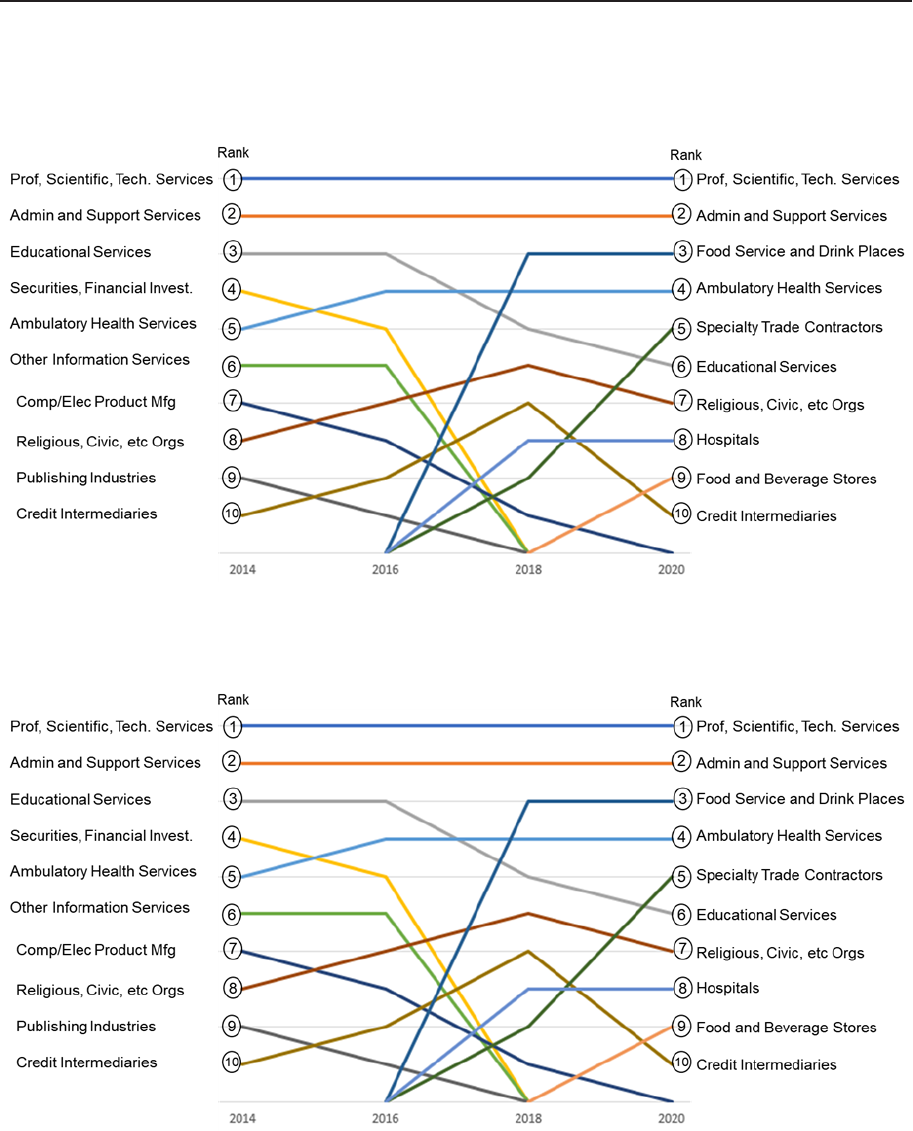
Hoopes, Menzer, and Wilde
FIGURE 6. Industry of CRYPTOCURRENCY SELLERs over time
PANEL A: Top CRYPTOCURRENCY SELLER Job Industries Over Time by Percentage
PANEL B: Top CRYPTOCURRENCY SELLER Job Industries Over Time by Number
Note: Panel A presents the ratio of CRYPTOCURRENCY SELLERs in a particular business industry by year compared to all taxpayers in the given industry, Panel B pres-
ents the top business industries over time ranked by the number of CRYPTOCURRENCY SELLERs. To identify industry of a taxpayer, we obtain the population of W-2 data
for our sample years, which reports wage income and use the W-2 with the highest reported income each year. Next, we identify the three-digit NAICS code based on the
business tax return that led the Form W-2. Since CRYPTOCURRENCY SELLER is calculated at the tax return level, if a joint tax return is led, we assume both spouses
are/are not holders of cryptocurrency. The denominator is the total taxpayers whose highest paid W-2 is in the given industry. Each taxpayer is assigned only a single indus-
try. Data points are for each even numbered year between 2014 and 2020. A point at the bottom of each chart means that the specied industry was not in the top 10.

Who Sells Cryptocurrency?
TABLE 1. Descriptive Statistics
Variables of Interest
NON-INVESTOR
(N=845,102,236)
NON-CRYPTOCURRENCY INVES-
TOR (N=230,965,310)
CRYPTOCURRENCY SELLERS
(N=2,620,926)
Mean Std. Dev. Median Mean Std. Dev. Median Mean Std. Dev. Median
AGE 41.47 16.72 39 56.26 18.52 58
32.78 10.75 30
WAGES 39,506 257,012 26,604 86,318 392,742 37,413
77,049 355,060 46,010
TAXABLE INTEREST 98 49,955 0 2,757 152,022 47
1,733 1,263,304 0
TAXABLE DIVIDENDS 0 0 0 7,882 267,688 469
1,649 81,328 0
SCH A 0.168 0.374 0 0.442 0.497 0
0.131 0.338 0
MARRIED 0.316 0.465 0 0.584 0.493 0
0.378 0.485 0
MALE 0.314 0.464 0 0.182 0.385 0
0.541 0.498 0
STUDENT 0.062 0.242 0 0.031 0.174 0
0.197 0.398 0
LN WAGES 8.877 3.611 10.19 7.491 5.263 10.53
9.724 3.309 10.74
LN DIVIDENDS - 0.000 0 5.663 3.194 6.15
1.686 2.690 0
Descriptive Variables
CAPITAL GAIN/LOSS* 0 0 0 22,512 856,090 24
18,765 1,167,616 0
TAXABLE INCOME 34,346 88,971 19,747 138,353 1,079,166 67,115
91,421 1,086,150 36,372
CRYPTOCURRENCY GAIN - -
12,484 824,804 27
NUM OF CRYPTO TRANSACTIONS - -
9.90 100.40 1
EIC TAX CREDIT 0.173 0.378 0 0.015 0.123 0
0.066 0.249 0
GAMBLER 0.009 0.096 0 0.010 0.099 0
0.009 0.094 0
CANCELLATION OF DEBT 0.018 0.134 0 0.007 0.085 0
0.017 0.129 0
CRYPTOCURRENCY 1099B - -
0.784 0.412 1
Note: Table 1 reports descriptive statistics for the full sample of taxpayers (2013-2020) split out between NON-INVESTORs, NON-CRYPTOCURRENCY SELLING INVESTORs, and CRYPTOCURRENCY SELLERs. CRYPTOCURRENCY
SELLERs are taxpayers who we identify as selling cryptocurrency for year t through textual analysis of Form 8949 Capital Gain descriptions, or who receive a Form 1099-B which we identify as relating to cryptocurrency through textual anal-
ysis of the description. NON-CRYPTOCURRENCY SELLING INVESTORs are taxpayers who are not identied as selling cryptocurrency but do report either Dividends or a Capital Gain or loss on their Form 1040 in year t. NON-INVESTOR
Taxpayers are all other taxpayers. CAPITAL GAIN/LOSS is limited to the 3,000 capital loss limitation, however, CRYPTOCURRENCY GAIN is calculated on a transaction level basis and is not calculated with regard to the overall capital gain
limitation. CRYPTOCURRENCY GAIN and NUM OF CRYPTO TRANSACTIONS are calculated only using information from Form 8949 and thus have limited non-missing observations (863,340 and 894,177 respectively). Some transactions
reported on Form 1099-B may be summarized by taxpayers on their Form 1040 or Schedule D, and thus we would not be able to identify reported amounts for those transactions from the tax return. We avoid calculating reported amounts
from Form 1099-B to avoid double counting transactions which are reported on both Form 8949 and Form 1099-B. SINGLE MALE and MARRIED are part of a categorical variable where the baseline is taxpayers who do not le a joint return
and are female. Medians are calculated as the mean of the observations around the median observation per IRS disclosure guidelines. Due to missing values for gender and age in the Social Security Administration database, a small
number of values for those amounts are missing. In order to comply with IRS data disclosure requirements, medians are calculated as a local average around the true median.

Hoopes, Menzer, and Wilde
TABLE 2. CRYPTOCURRENCY MILLIONAIRE descriptive statistics
NON-INVESTOR
NON-CRYPTOCUR-
RENCY INVESTOR
CRYPTOCURRENCY
SELLER
EQUITY MILLIONAIRE
CRYPTOCURRENCY
MILLIONAIRE
Mean
Std. Dev.
Mean Std. Dev. Mean Std. Dev. Mean Std. Dev. Mean Std. Dev.
Continuous Variables
AGE 41.47 16.72 56.26 18.52 32.69 10.67 46.76 13.37 40.53 11.49
WAGES 39,505 257,012 86,215 389,079 74,387 182,305 457,407 2,688,332 366,092 5,790,899
TAXABLE INTEREST 98 49,955 2,739 151,735 1,173 1,266,663 63,392 523,876 96,070 949,502
TAXABLE DIVIDENDS - - 7,853 267,254 797 24,845 102,780 513,208 165,186 2,225,614
CAPITAL GAIN/LOSS* - - 22,207 839,433 5,682 536,312 1,065,872 8,058,907 2,397,415 20,173,968
CRYPTOCURRENCY GAIN - - - - 3,402 33,204 -33,068 3,801,461 1,753,248 8,722,526
TAXABLE INCOME 34,345 88,960 137,908 1,068,095 74,386 355,173 1,699,424 8,233,654 2,833,299 16,598,034
NUM OF CRYPTO TRANSACTIONS - - - - 10 93 15 214 55 405
Indicator Variables
TAXABLE LTCG 0.000 0.002 0.435 0.496 0.196 0.397 0.517 0.500 0.493 0.500
SCH A 0.168 0.374 0.442 0.497 0.127 0.333 0.805 0.396 0.569 0.495
EIC TAX CREDIT 0.173 0.378 0.015 0.123 0.067 0.250 0.002 0.049 0.006 0.078
MARRIED 0.316 0.465 0.584 0.493 0.375 0.484 0.747 0.435 0.559 0.497
MALE 0.314 0.464 0.182 0.385 0.543 0.498 0.223 0.416 0.414 0.493
CRYPTOCURRENCY 1099B - - - - 0.789 0.408 0.026 0.158 0.024 0.154
STUDENT 0.06 0.24 0.03 0.17 0.198 0.399 0.018 0.132 0.027 0.163
GAMBLER 0.01 0.10 0.01 0.10 0.009 0.094 0.012 0.108 0.015 0.122
CANCELLATION OF DEBT 0.02 0.13 0.01 0.09 0.017 0.129 0.005 0.069 0.006 0.080
Note: These statistics are for the full sample of taxpayers (2013-2020) split out between NON-INVESTORs, NON-CRYPTOCURRENCY SELLING INVESTORs, CRYPTOCURRENCY SELLERs, EQUITY MILLIONAIREs, and CRYPTOCUR-
RENCY MILLIONAIREs. CRYPTOCURRENCY MILLIONAIRE is a time invariant indicator for taxpayers who recognize over $1 million of gain as a result of cryptocurrency transactions over the sample period. EQUITY MILLIONAIRE is a
time invariant indicator for taxpayers who recognize over $1 million of equity capital gain and do not recognize over $1 million of cryptocurrency gain. CAPITAL GAIN/LOSS is limited to the $3,000 capital loss limitation; however, CRYPTO-
CURRENCY GAIN is calculated on a transaction level basis and is not calculated with regard to the overall capital gain limitation. CRYPTOCURRENCY GAIN and NUM OF CRYPTO TRANSACTIONS are calculated only using information
from Form 8949 and thus have limited non-missing observations (863,340 and 894,177 respectively). Some transactions reported on Form 1099-B may be summarized by taxpayers on their Form 1040 or Schedule D, and thus we would
not be able to identify reported amounts for those transactions from the tax return. We avoid calculating reported amounts from Form 1099-B in order to avoid double counting transactions which are reported on both Form 8949 and Form
1099-B. SINGLE MALE and MARRIED are part of a categorical variable where the baseline is taxpayers who do not le a joint return and are female. Medians are calculated as the mean of the observations around the median observation
per IRS disclosure guidelines. Due to missing values for gender and age in the Social Security Administration database, a small number of values for those amounts are missing.

Who Sells Cryptocurrency?
TABLE 3. Top 10 Cryptocurrency Cities for 2014 and 2020
PANEL A. Top Cryptocurrency Cities for 2014 and 2020 by Percentage of Taxpayer Returns
2014 2020
Rank City Percentage of Sellers Rank City Percentage of Sellers
1
Menlo Park, CA
0.0637% 1
Sunnyvale, CA
1.5402%
2
Mountain View, CA
0.0522% 2
Mountain View, CA
1.5245%
3
San Francisco, CA
0.0410% 3
Ross, CA
1.4648%
4
Palo Alto, CA
0.0384% 4
Milpitas, CA
1.4638%
5
Redmond, WA
0.0369% 5
Cupertino, CA
1.4595%
6
Cambridge, MA
0.0304% 6
Santa Clara, CA
1.4430%
7
New York, NY
0.0202% 7
Redmond, WA
1.4292%
8
Fremont, CA
0.0187% 8
Fremont, CA
1.4005%
9
Seattle, WA
0.0147% 9
Dublin, CA
1.3889%
10
Plano, TX
0.0137% 10
Secaucus, NJ
1.3819%
PANEL B. Top Cryptocurrency Cities for 2014 and 2020 by Number of Taxpayers
2014 2020
Rank City Number of Sellers Rank City Number of Sellers
1 San Francisco, CA 162 1 Brooklyn, NY 5,425
2 New York, NY 158 2 New York, NY 5,358
3 Seattle, WA 60 3 Los Angeles, CA 4,775
4 Brooklyn, NY 59 4 Chicago, IL 4,683
5 Austin, TX 47 5 San Francisco, CA 4,450
6 Los Angeles, CA 42 6 Houston, TX 3,912
7 Houston, TX 42 7 Austin, TX 3,880
8 Chicago, IL 41 8 Seattle, WA 3,643
9 San Jose, CA 30 9 San Jose, CA 3,593
10 Minneapolis, MN 30 10 San Diego, CA 3,546
Note: Panel A shows the top ten cities based on the percentage of CRYPTOCURRENCY SELLER tax returns led in the given city over all tax returns led in the given city. The percentage is not calculating the number of taxpayers as one
tax return may relate to either one or two taxpayers given the ling status. Panel B shows the top ten cities based on the total number of CRYPTOCURRENCY SELLER tax returns led in the given city. For both panels, we require any given
city to have at least 1,000 tax returns led in the year, and at least 10 CRYPTOCURRENCY SELLER returns led in the year to reduce extreme percentages and due to IRS data restrictions. Taxpayer city is dened using taxpayer provided
information on the Form 1040.

Hoopes, Menzer, and Wilde
TABLE 4. Top Cryptocurrency Job Industries for 2014 and 2020
PANEL A. Top Cryptocurrency Job Industries for 2014 and 2020 by Percentage
2014 2020
Rank
Industry NAICS3 Percent Industry NAICS3 Percent
1
Other Information Services 519 0.04% Other Information Services 519 3.29%
2
Securities, Commodity Contracts, and Other
Financial Investments and Related Activities
523 0.02% Internet Publishing and Broadcasting 516 2.70%
3
Data Processing, Hosting, and Related Services 518 0.02% Data Processing, Hosting, and Related Services 518 2.61%
4
Publishing Industries (except Internet) 511 0.01% Publishing Industries (except Internet) 511 2.15%
5
Computer and Electronic Product Manufacturing 334 0.01% Electronics and Appliance Stores 443 2.04%
6
Professional, Scientic, and Technical Services 541 0.01% Professional, Scientic, and Technical Services 540 1.91%
7
Museums, Historical Sites, and Similar
Institutions
712 0.01% Computer and Electronic Product Manufacturing 334 1.76%
8
Motion Picture and Sound Recording Industries 512 0.01% Nonstore Retailers 454 1.73%
9
Funds, Trusts, and Other Financial Vehicles 525 0.01% Telecommunications 517 1.72%
10
Telecommunications 517 0.00% Information 510 1.65%
PANEL B: Top Cryptocurrency Job Industries for 2014 and 2020 by Number
2014 2020
Rank
Industry NAICS3 Number Industry NAICS3 Number
1 Professional, Scientic, and Technical Services 541 943 Professional, Scientic, and Technical Services 541 227,586
2 Administrative and Support Services 561 301 Administrative and Support Services 561 141,207
3 Educational Services 611 248 Food Services and Drinking Places 722 98,763
4 Securities, Commodity Contracts, and Other
Financial Investments and Related Activities
523 212 Ambulatory Health Care Services 621 71,381
5 Ambulatory Health Care Services 621 191 Specialty Trade Contractors 238 56,926
6 Other Information Services 519 143 Educational Services 611 55,423
7 Computer and Electronic Product Manufacturing 334 124 Religious, Grantmaking, Civic, Professional, and
Similar Organizations
813 41,559
8 Religious, Grantmaking, Civic, Professional, and
Similar Organizations
813 121 Hospitals 622 39,738
9 Publishing Industries (except Internet) 511 108 Food and Beverage Stores 445 39,737
10 Credit Intermediation and Related Activities 522 107 Credit Intermediation and Related Activities 522 33,102
Note: Table 4, Panel A presents the ratio of Cryptocurrency Sellers in a particular business industry by year compared to all taxpayers in the given industry. To identify industry of a taxpayer, we obtain the population of W-2 data for our
sample years, which reports wage income and use the W-2 with the highest reported income each year. Next, we identify the three-digit NAICS code based on the business tax return that led the Form W-2.. Since CRYPTOCURRENCY
SELLER is calculated at the tax return level, if a joint tax return is led, we assume both spouses are/are not holders of cryptocurrency. The denominator is the total taxpayers whose highest paid W-2 is in the given industry. Each taxpayer is
assigned only a single industry. Panel B presents the same information except that instead of the ratio of CRYPTOCURRENCY SELLER s total, industries are ranked by the raw number of CRYPTOCURRENCY SELLER s.

Who Sells Cryptocurrency?
TABLE 5. Determinants of CRYPTOCURRENCY SELLER
Independent Variables
Dependent Variable: CRYPTOCURRENCY SELLER
Model 1 Model 2
Estimate Std. Error † Estimate Std. Error †
AGE (UNDER 24) 0.00458 (0.000062) 10 -0.00395 (0.000068) 10
AGE (25-44) 0.00466 (0.000054) 10 -0.00372 (0.000058) 10
AGE (45-64) 0.00113 (0.000036) 10 -0.00073 (0.000039) 10
LN WAGES 0.00006 (0.000004) 10 -0.00004 (0.000005) 10
LN DIVIDENDS 0.00035 (0.000007) 10 -0.00021 (0.000007) 10
MARRIED 0.00247 (0.000035) 10 -0.00333 (0.000057) 10
SINGLE MALE 0.00353 (0.000041) 10 -0.00482 (0.000066) 10
HOMEOWNER 0.00029 (0.000036) 10 -0.00012 (0.00004) 6
DEPENDENTS -0.00031 (0.000017) 10 0.00032 (0.000019) 10
STUDENT 0.00380 (0.000126) 10 -0.00487 (0.00016) 10
TREND -0.00140 (0.000018) 10
AGE (UNDER 24) * TREND 0.00232 (0.000034) 10
AGE (25-44) * TREND 0.00227 (0.000028) 10
AGE (45-64) * TREND 0.00048 (0.000018) 10
LN WAGES * TREND 0.00002 (0.000002) 10
LN DIVIDENDS * TREND 0.00015 (0.000003) 10
MARRIED * TREND 0.00125 (0.000019) 10
SINGLE MALE * TREND 0.00179 (0.000022) 10
HOMEOWNER * TREND 0.00011 (0.00002) 10
DEPENDENTS * TREND -0.00018 (0.00001) 10
STUDENT * TREND 0.00163 (0.000053) 10
Intercept -0.00031 (0.000017) 10 0.00032 (0.000019) 10
Observations 10,000,000 10,000,000
Year Fixed Eects YES NO
Baseline Full Sample Probability of Crypto
Seller
0.00243 0.00243
Average Adjusted R2
0.002 0.002
† The number of signicant coecients (out of 10) at the 1% level across the 10 random samples.
Note: Reported coecient estimates, standard errors, and adjusted R
2
are average numbers over 10 iterations of random sampling. For each random sample, 10 million
tax returns were selected at random from the full sample of tax returns (approx. 1.078 billion, from which the baseline full sample probability was computed). Numbers to the
right of the coecient are the number of coecients that were signicant at the 1% level over all iterations. Column (1) reports the results of model 1 on a random sample
of all tax returns. Column (2) reports the results of model 2 on a random sample of all tax returns. Variables are dened in Online Appendix A. Robust Standard errors are
reported in parentheses. To aid in the interpretation of coecient magnitude, the baseline full sample probability of being a CRYPTOCURRENCY SELLER is reported at the
bottom of each column.

Hoopes, Menzer, and Wilde
TABLE 6. Cross Sectional Samples of Cryptocurrency Determinants
Dependent Variable: CRYPTOCURRENCY SELLER
Sample (1) Sample (2) Sample (3) Sample (4)
Early Sample
2013-2016
Late Sample
2017-2020
Only Crypto
Sellers and
Investors
Only Crypto
Sellers and
non-Investors
Independent Variables
Estimate
(Std. Error)
†
Estimate
(Std. Error)
†
Estimate
(Std. Error)
†
Estimate
(Std. Error)
†
AGE (UNDER 24) 0.00004 8 0.00850 10 0.03255 10 0.00380 10
(0.000012) (0.000117) (0.000574) (0.000063)
AGE (25-44) 0.00007 10 0.00856 10 0.02076 10 0.00348 10
(0.000013) (0.000098) (0.000272) (0.000053)
AGE (45-64) 0.00004 7 0.00189 10 0.00090 10 0.00064 10
(0.000012) (0.000064) (0.000135) (0.000039)
LN WAGES 0.00000 1 0.00010 10 0.00011 10 0.00004 10
(0.000001) (0.000008) (0.000015) (0.000005)
LN DIVIDENDS 0.00002 10 0.00062 10 -0.00342 10 0.16578 10
(0.000002) (0.000012) (0.000029) (0.00085)
MARRIED 0.00003 10 0.00469 10 0.00694 10 0.00256 10
(0.000006) (0.000067) (0.000137) (0.00004)
SINGLE MALE 0.00004 10 0.00661 10 0.01865 10 0.00327 10
(0.000006) (0.000076) (0.000257) (0.000041)
HOMEOWNER 0.00001 2 0.00051 10 -0.00788 10 0.00029 10
(0.000007) (0.000069) (0.000155) (0.000041)
DEPENDENTS 0.00000 2 -0.00058 10 0.00006 0 -0.00030 10
(0.000003) (0.000033) (0.000096) (0.000017)
STUDENT 0.00000 0 0.00413 10 0.02613 10 0.00363 10
(0.000016) (0.000163) (0.000912) (0.000126)
Intercept 0.00000 2 -0.00058 10 0.00006 0 -0.00030 10
(0.000003) (0.000033) (0.000096) (0.000017)
Observations 10,000,000 10,000,000
Year Fixed Eects YES YES YES YES
Baseline Full Sample Prob-
ability of Crypto Seller
0.00004 0.00459 0.00309 0.01122
Average Adjusted R
2
0.000 0.005 0.011 0.003
† The number of signicant coecients (out of 10) at the 1 percent level across the 10 random samples.
Note: Reported coecient estimates, standard errors, and adjusted R
2
are average numbers over 10 iterations of random sampling. For each random sample, 10 million
tax returns were selected at random from the full sample of tax returns (approx. 1.078 billion, from which the baseline full sample probability was computed). Numbers to
the right of the coecient are the number of coecients that were signicant at the 1 percent level over all iterations. Columns (1) and (2) report the results of model 1 run
on the same random samples split by early sample period (2013-2016) and late sample period (2017-2020). Each column is therefore only a portion of the full 9 million
tax return random sample. Columns (3) and (4) report the results of model 1 where the control sample consists of only NON-CRYPTO SELLING INVESTORs (3) or NON-
INVESTORs (4). Each column is therefore only a portion of the full 10 million tax return random sample. Variables are dened in Online Appendix A. Robust standard errors
are reported in parenthesis. To aid in the interpretation of coecient magnitude, the baseline full sample probability of being a CRYPTOCURRENCY SELLER is reported at
the bottom of each column. The number of observations in each random sample varies based on the cross-sectional split and random sample.

Who Sells Cryptocurrency?
Online Appendix—Not for print publication
Overview of the Bitcoin Network and Transactions
Bitcoin can refer both to the unit of account as well as the ledger which records transactions denominated in
Bitcoin. Although we will discuss Bitcoin specically, the general information applies to many other similar
cryptocurrencies, and we attempt to note important dierences. Bitcoin is a decentralized public ledger and
can be thought of as serving a similar function to a bank. e Bitcoin ledger, commonly referred to as “the
blockchain,” contains and updates a list of transactions which can be used to identify how much Bitcoin is as-
sociated with each account. We next go over the key features of Bitcoin and similar cryptocurrencies.
Unlike a traditional bank, Bitcoin is decentralized. is means there is no central authority approving or
processing transactions. Instead, when an individual wants to send Bitcoin, they broadcast the transaction to
the entire Bitcoin network. en, individuals or groups known as “Miners” observe those transactions and
compete with each other for the right to conrm those transactions are legitimate and post them to the block-
chain. is competition helps to ensure that no single entity has control over which transactions are or are not
posted to the ledger. As a reward for the eort, miners are rewarded with both Bitcoin transaction fees paid by
users, as well as a set Bitcoin reward which is created for each new batch of transactions that is conrmed. For
Bitcoin, the competition for the right to post transactions is based on computing power, where miners with
more computing power are more likely to win. Other cryptocurrencies use other mechanisms to determine
which transactions are recorded on the blockchain.
Although the blockchain is a form accounting ledger, there are several dierences which make it unique
from other systems. First, the blockchain does not record running totals like a bank account. Instead, each ac-
count (also called a wallet) is the sum of all transactions that have taken place relating to that wallet. erefore,
in order to know the current balance of a wallet, one must examine the entire history of the blockchain, not
simply the most recent transactions. e second dierence is that Bitcoin accounts cannot be split. If a user has
Bitcoin in a wallet and want to spend Bitcoin, then they must send Bitcoin to another wallet owned
by themselves and Bitcoin to the external recipient. Wallets are reusable and can receive unlimited deposits.
e third detail about Bitcoin is that it is a sender-based system. In order to send Bitcoin, all a sender needs is
a Bitcoin account address, and Bitcoin can be sent without any action or even knowledge of the receiver. Taken
together, this makes Bitcoin pseudonymous. e entire transaction history of each individual Bitcoin account
can be observed, however, a single user can have an innite number of accounts. In addition, because there is
no central processing party, the identity of the owner of individual Bitcoin accounts is dicult to determine
without additional information outside of the blockchain.
Several factors have led to innovation and changes within the cryptocurrency space. First, long transac-
tion approval times (greater than minutes for many Bitcoin transactions) and high transaction fees have led
users to both transact with centralized Bitcoin market makers and develop competing cryptocurrencies with
the aim of reducing the ineciencies in Bitcoin. Second, although Bitcoin is pseudonymous, newer cryptocur-
rencies have been designed to increase privacy and security. Finally, new blockchains have been developed
which allow users to increase the complexity of transactions. For example, a user could set up a transaction
to send some value of cryptocurrency only if a specic set of identiable outcomes is realized. Ultimately, the
Bitcoin and cryptocurrency ecosystem continues to rapidly evolve and change over time, oering new oppor-
tunities but also challenges for investors, regulators, and researchers.
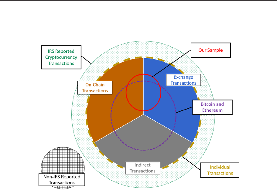
Hoopes, Menzer, and Wilde
ONLINE Appendix Figure 1. Cryptocurrency Transaction Types (Not drawn
to scale)
Notes: is gure is a representation of the various types of cryptocurrency transactions that taxpayers may
engage in and how those denitions relate to our sample of identied cryptocurrency transactions. e gure
is not intended to be denitive but is provided to help understand the relationship between the universe of
transactions and those which we identify. We provide additional denitions below:
Non-IRS Reported Transactions: ese are cryptocurrency transactions which are not reported to the IRS on
an individual tax return on Form nor are reported to the IRS by third parties on Form -B.
IRS Reported Cryptocurrency Transactions: ese are transactions which are reported to the IRS. is could
be through reporting on tax returns (Individual, Business, and Trust), or through reported to the IRS through
various third-party reporting (e.g., Form -B, Form -MISC).
Individual Transactions: ese transactions include only those transactions that are reported directly on
Form for an individual taxpayer or are reported on Form -B where the taxpayer has a Social Security
Number. Individual transactions do not include transactions which are reported by businesses even if those
transactions may eventually ow through to an individual return on Schedule K- and Schedule E.
On-Chain Transactions: On-Chain transactions refer to cryptocurrency transactions which are recorded
permanently on a public blockchain. ese transactions include sending or receiving cryptocurrency directly
to individual wallets as well as sales of cryptocurrency made directly on the blockchain. e details of these
transactions is generally publicly available but pseudo-anonymous. It is thus dicult to link the public block-
chain data directly to taxpayers. On-Chain Transactions also are not generally subject to third-party reporting
unless there is a centralized intermediary facilitating the transaction.
Exchange Transactions: Exchange transactions refer to cryptocurrency transactions done through a central-
ized third-party outside of the blockchain. ese transactions are generally recorded on internal accounts or
ledgers of the centralized party. us, individual transactions may not appear, or may only appear in aggregate
on the blockchain.

Who Sells Cryptocurrency?
ONLINE Appendix Figure 2. Google Trends Index for “bitcoin”

4
∇
Hidden Assets, Hidden Networks
Wind Bratt Gra Herlache
King Soto Yismaw Doyle Horvath Nowicki
Hess Gleason Sundstrom Brooks Mastrangelo
Stavrianos Hales

Following K-1s: Considering Foreign
Accounts in Context
Tomas Wind, David Bratt, Alissa Gra, and Anne Herlache
(IRS: Research, Applied Analytics, and Statistics)
1
I. Introduction
U.S. taxpayers’ use of oshore accounts has been an area of focus for the IRS for some time. ere are several
reasons why this is the case. First, given the requirement that U.S. taxpayers pay taxes to the IRS regardless of
their country of residence,
assets in overseas accounts held by taxpayers living outside of the United States
may generate income that is legally subject to U.S. taxes. Second, and more signicantly, foreign nancial in-
stitutions’ historically limited reporting of U.S. taxpayers’ overseas assets to the IRS means that taxpayers who
hold or move assets overseas may be underreporting their assets, thereby, not remitting the full amount of the
U.S. taxes that they owe. For these and other reasons, the IRS has long implemented programs in its criminal
investigatory and civil components to increase the number of U.S. taxpayers with overseas assets who come
into and stay in compliance with the U.S. tax laws that pertain to their overseas assets.
Such compliance is a dicult task to ensure. In addition to the fact that some U.S. taxpayers who reside
overseas may be unaware of their obligation to report their overseas assets to the IRS, recent immigrants to the
U.S. who are obliged to pay taxes on their overseas accounts to the IRS may also be unaware of their need to do
so. Moreover, the gaps in relevant reporting from overseas nancial institutions described above makes it di-
cult for U.S. tax authorities to clearly understand the holdings of U.S. persons with overseas assets. And, nally,
this murky picture is further clouded by the rise of the use of pass-through entities in a variety of tax scenarios.
In light of these challenges, the IRS’s civil component has implemented several pathways over the past
twentysomething years for those persons who owed U.S. taxes on their overseas holdings but had previously
not reported these assets to the IRS to voluntarily come into compliance with U.S. tax law. While each of these
programs (which are summarized below in Section II) had dierent criteria for participation, they generally
allowed such persons to avoid the signicant criminal penalties that they may have faced if their noncompli-
ance had been discovered by IRS Criminal Investigations (CI). In doing so, they have made a substantial im-
pact on the estimated size of the noncompliant population of U.S. persons with overseas assets.
While the particularities of U.S. tax law shaped the specics of these initiatives, they were not rolled out in
global isolation. Indeed, the Organisation for Economic Co-operation and Development, G, and other in-
ternational bodies made signicant strides during this same time period to promote transparency in countries
whose opaque nancial industries masked potential noncompliance with tax laws on the part of citizens of a
variety of countries. ese eorts to combat tax evasion have been and continue to be an important backdrop
to eorts undertaken by the IRS.
Our paper examines one dynamic by which these initiatives may have had their ultimate eect on the
population of noncompliant U.S. persons. In particular, we examine the inuence of those who reported a
foreign account during – on those other U.S. persons with whom they are linked through what we
will refer to as a K- network. We show that a relationship exists between sharing a network with taxpayers that
have reported a foreign account and reporting a foreign account.
1
disclosed.
2
Filing requirements for U.S. citizens or resident aliens living or traveling outside the United States is determined by the amount of gross income from worldwide
3
For an overview of these related international eorts, see “A Step Change in Tax Transparency” (OECD 2013).

Wind, Bratt, Gra, and Herlache
II. Background on Foreign Account Reporting
Report of Foreign Bank and Financial Accounts
e Bank Secrecy Act (BSA) of stipulates that some U.S. persons must le a Report of Foreign Bank and
Financial Account a.k.a. “FBAR” (FinCEN Form ). ose persons include a citizen, resident, corporation,
partnership, LLC, trust, or estate that have a nancial interest in or authority over one or more overseas ac-
counts. In keeping with other portions of the BSA, this reporting requirement only applies if the aggregate val-
ue of the foreign accounts of the U.S. person in question is greater than , in the calendar year in which
it was reported.
U.S. persons who are required to le an FBAR must do so by submitting FinCEN Report
(which replaced TD Form -. in ).
Foreign Account Tax Compliance Act
e Foreign Account Tax Compliance Act (FATCA) was passed in as part of the Hiring Incentives to
Restore Employment Act. In requiring certain U.S. persons and entities to report their foreign account hold-
ings, FATCA is broadly similar to FBAR. However, FATCA has a higher asset-reporting threshold , to
, (depending on residence and marital status). It does not apply to U.S. persons in U.S. territories, and
its denition of assets is broader than that covered by FBAR. In particular, FATCA requires the reporting of
foreign stocks and securities, foreign nancial instruments, contracts with non-U.S. persons, and other inter-
ests in foreign entities.
Oshore Voluntary Disclosure Programs
We use “OVD” (Oshore Voluntary Disclosure) to refer to a series of four initiatives that the IRS undertook
from –.
ese initiatives built o of CI’s longstanding practice of taking voluntary disclosures under
consideration when determining whether to recommend criminal prosecution. Across the four iterations of
OVD, the IRS used an evolving set of incentives (in the form of reduced civil penalties and, in most cases, the
waiver of criminal liability) to encourage taxpayers with overseas nancial accounts and assets to come into
compliance with US tax law.
e dates for each iteration of the OVD are as follows:
• –October 8, 2009
• –September 9, 2011
• –
• –technically a continuation of the 2012 program, but
with signicant modications)
By assessing penalties on the accounts and assets covered by this program, the IRS thereby encouraged a
subset of those who had been willfully noncompliant, U.S. taxpayers looking overseas who were unaware of
their U.S. tax obligations, so-called “quiet disclosers,” and others to come into compliance with U.S. tax law.
At the end of a successfully completed OVD ling, the taxpayer would enter into a Specic Matters Closing
Agreement with the IRS.
4
This overview is based on and, in some places, directly quotes the IRS’s overview of . There are several
5
Summary of FATCA Reporting for U.S. Taxpayers | Internal Revenue Service (irs.gov), Foreign Account Tax Compliance Act (FATCA): Denition and Rules
(investopedia.com).
6
ere was a related program in 2003 called the “Oshore Voluntary Compliance Initiative” that in some ways was a precedent for what we call the “OVD
programs.” However, its penalty structure was dierent enough, the reported disclosures of the program small enough, and the geopolitical context was dierent
enough from the OVD programs from 2009 on that we exclude it from our analysis. For a comparison of the penalty structures of these programs including the
2003 OVCI), see GAO (2013).
7
For a summary of the provisions and history of OVDP, see IRM 4.63.3.1.

Following K-1s: Considering Foreign Accounts in Context
Streamlined Filing Compliance Procedures
While OVD’s target population included taxpayers whose noncompliance was at least in part willful, the
Streamlined Filing Compliance Procedures (SFCP) were aimed at those whose noncompliance was completely
non-willful. is program began on September , , and is still available to those who believe that they may
have been non-willfully noncompliant with U.S. tax law. SFCP was designed to complement OVD, as many
taxpayers who were non-willfully noncompliant were entering OVD and then withdrawing from the program
aer determining that the program’s penalty structure was not appropriate for their situation.
Aer SFCP was
set up and while OVDP was still running, taxpayers had to make a mutually exclusive choice for one or the
other paths to compliance.
In certifying that their noncompliance was not willful, taxpayers who hope to avail themselves of SFCP
attested that their noncompliance was the result of their “negligence, inadvertence, or mistake or conduct
that is the result of a good-faith misunderstanding of the requirements of the law.”
While the streamlined
ling procedure was initially available only to U.S. taxpayers residing abroad, the IRS subsequently opened
this program up to U.S. taxpayers residing in the United States as well. e two dierent sets of procedures
are known, respectively, as the “Streamlined Foreign Oshore Procedures” and the “Streamlined Domestic
Oshore Procedures” (SDO). Aside from the dierence in residency status, they diered primarily in that
SDO imposes a ve-percent so-called “miscellaneous oshore penalty.”
III. Literature Review
Work on Pass-through Entities and Network Analysis
Pass-through entities (PTEs) have the dual character of being required to submit a tax return while not them-
selves being subject to federal income tax. is function of passing the income (and the attendant tax obliga-
tion) that comes into the PTE on to its constituent members makes this entity structure an attractive option
in a variety of dierent tax planning scenarios. As such, PTEs and the resulting K- networks that they create
have become more widely employed by U.S. taxpayers. (See Olson et al. (), p. - for a more detailed dis-
cussion of this topic.) ey have also been the subject of a good deal of analysis by academics, tax authorities,
and other interested parties.
Since the seminal work of Cooper et al.in their paper on pass-through entities, scholars have made
innovative use of K- network data in their analysis of various aspects of tax administration in the United
States (Cooper et al. (). In “Entity Structure and Taxes: An Analysis of Embedded Pass-rough Entities,”
for example, the authors demonstrate that the passthrough entities are more likely to appear in relatively com-
plex corporate structures. ey also show that the presence of PTEs in corporate structures is “signicantly
associated” with tax avoidance and uncertainty (Agarwal et al. (), p. ). While the scope of their study is
limited to C-corporations, the authors’ analysis demonstrates the power of K- networks as a tool for analyzing
such data and assisted us in developing a number of metrics used in this paper.
An earlier paper (Agarwal et al. ()) by a subset of the same authors and other collaborators within the
IRS demonstrates another way to protably analyze K- network data. In particular, the authors of this paper
show how one can analyze taxpayer networks linked by K-s through the lens of social network analysis. In
indexing the types and numbers of entities within K- networks and the dierent types of linkages between
them, this paper denes typical network structures and identies anomalous pass-through arrangements that
may be of interest to tax authorities. Recent work (Love ()) has given a more rened description of the
specic entities, dynamics, and capital ows that appear within K- networks. Aer observing that Cooper et
al.were able to identify the ultimate recipients of percent of the income owing through the universe of K-
data reported to the IRS, Love uses an expanded set of data points and tailored algorithms to attribute most of
the income that Cooper et al.had been unable to pin down. (Love estimates that he is able to account for
8
https://www.irsvideos.gov/business/FilingPayingTaxes/StreamlinedFilingComplianceProceduresAComplianceOptionForSomeTaxpayers.
9.
Streamlined Filing Compliance Procedures | Internal Revenue Service (irs.gov).

Wind, Bratt, Gra, and Herlache
percent of the total income owing through this space.) Love shows that much of this newly revealed activity is
) associated with the nancial industry, ) makes use of a so-called “blocker entity” that is domiciled overseas
and which reduces and/or redirects its owners’ tax liability, and ) largely directs capital from the U.S. to for-
eign partners. Given the opacity of the operations of such blocker entities, the nal beneciaries of such ows
are unclear, but Love suggests that the general ow of passive investment income from the U.S. to overseas
partners has deleterious eects that must be weighed against the benets of the inows of foreign investment
into the U.S. that are also facilitated by U.S. tax policy.
Black et al.() further advances our understanding of the landscape of partnerships that report to
the IRS. Using various forms of graphical analysis to visualize the structure of partnership arrangements and
the capital ows within them, Black et al suggest a general division of partnerships into simple, single-owner
structures on one hand and complex structures with multiple owners on the other. Suggesting that the two
constitute, respectively, percent and percent of the total population of partnerships, Black et al. show that
this smaller group of complex partnerships is characterized by circular ownership structures in a given part-
nership as well as multidirectional ows of capital therein. In terms of methodology, the authors demonstrate
that random forest models outperform traditional linear regressions in terms of the accuracy of each predicted
noncompliance.
Work on Foreign Accounts
In addition to the research on K- networks outlined above, there have also been several studies on the eect of
the range of initiatives that the IRS has taken over the past twenty years to increase taxpayer compliance with
reporting requirements for overseas accounts. One notable early study of the eect of the earlier iterations of
the Oshore Voluntary Disclosure programs (hereaer referred collectively as “OVD”; see section II above for
a more detailed description of the chronology of the various iterations of this program) was produced by the
Government Accountability Oce (GAO) in (GAO ()). e GAO report makes several points that
were amplied by later academic research.
First, GAO notes that almost all of the participants in the iteration of OVD received the maximum
penalty possible under the program. Additionally, the authors note that most of these accounts were high-val-
ue accounts that were located in Switzerland. Moreover, they note that the iteration of OVD had broader
reporting requirements for participants; GAO suggests that this is because the data the IRS received from
earlier iterations of OVD did not provide sucient information to fully understand the landscape of overseas
noncompliance. Finally, GAO notes that there is reason to suspect that there were many U.S. taxpayers with
unreported foreign assets who amended their lings for previous years without participating in OVD. is
population of so-called “quiet disclosers,” GAO suggests, pose a specic risk for noncompliance.
Johannesen et al.() dives deeper into this same set of issues and provides analysis that includes several
additional years of data. e authors show that OVD did result in a signicant increase in compliance, but
that they argue that the relatively narrow scope of the program may mean that the more robust enforcement
mechanisms of FATCA were, in fact, warranted. e authors make their case by analyzing the enforcement
eect that is reected in data on OVD, in particular, and compare it to the data on populations, such as the
“quiet disclosers” that the Government Accountability Oce identied that are not included in that group.
e authors conrm the GAO’s ndings that, among those who came into compliance with U.S. tax law on
overseas assets during this period, OVD participants tended to have higher-value accounts.
ey also validate
the GAO’s concern about the population of quiet disclosers, as they suggest that the total amount of additional
tax remitted by quiet disclosers was much larger than the value of additional tax remitted by those who par-
ticipated in OVD. ey further estimate that the combined eect of these programs led to the disclosure of
roughly , additional accounts and billion in new wealth. By way of conclusion, Johannesen et al.
10
et al.
11
ey also conrm that many of the OVD accounts in the early 2009 and 2012 iterations of the program were located in Switzerland, Liechtenstein, and
Luxembourg. ey attribute this to the fact that nancial institutions in these countries were subject to heightened scrutiny and reporting requirements beginning
in the late 2000s. For a detailed overview of this background, see Johannesen et al.(2019) p. 1-9).

Following K-1s: Considering Foreign Accounts in Context
() suggest that the relatively narrow scope of OVD and the noncompliance that OVD did not address may
warrant the more robust reporting requirements of FATCA.
Johannesen et al. () looks at the early data that has emerged from FATCA to show the additional light
that this initiative shines on the details of U.S. taxpayer assets held overseas. By requiring that foreign nancial
institutions report on the owner(s), holdings within, and particular uses of the accounts of U.S. taxpayers over-
seas, FATCA greatly increases the amount of information available to the IRS about U.S. taxpayers’ overseas
wealth. us, despite issues with data quality and additional potential forms of noncompliance that FATCA
does not address, the authors conclude that FATCA and other administrative data show that U.S. taxpayers
hold roughly trillion dollars overseas. ey further note that this ownership is ) highly concentrated at the
very top (. percent) of the income spectrum and that ) roughly trillion of these assets are held in tradi-
tional tax havens. ey conclude by suggesting the need to better understand the eect that FATCA has on the
levels of voluntary compliance among taxpayers holding assets overseas.
IV. Graph Construction
We use IRS administrative data, which contains de-identied taxpayer data extracted from led tax returns,
enforcement information, and narrative data to construct a graph. Specically, we observe data extracted from
Form Schedule K-, Form S Schedule K-, and Form Schedule K- to identify taxpayer networks;
and from Form to examine reported individual income and spousal relationships. Finally, to identify tax-
payers with foreign accounts, we rely on FBAR data, Forms and , and voluntary disclosure programs
ling information.
Building Out K-1 Graphs
e primary structure of the graph relies on the relationship between K- recipients (payees) and K- issuers
(payers). We began by developing a graph for every year between and using data obtained from
Forms Schedule K-, S Schedule K-, and Schedule K-. Each graph contains two types of nodes
that represent payees and payers, as well as edges connecting payees and payers. Each edge contains data on
the total payment reported on the K-, which is used to calculate a proxy for ownership of the issuing entity
(i.e., partnership in the case of Form Schedule K-, S-corporation in the case of Form S Schedule K-
and trust for Form Schedule K-). Ownership is estimated by dividing the absolute value of the gains and
losses reported to a given payee by the sum of the absolute value of all gains and losses issued by the payer. We
created a subset graph to keep only edges that represent at least a percent stake by the payee. We took this step
to limit the size of the graph for computational purposes, as well as a means to restrict associations between
taxpayers to those that are more likely to be signicant.
We then constructed a separate graph consisting of taxpayers with reported foreign accounts and their
spouses. Taxpayers that reported holding foreign accounts in FBAR lings,
Form , and in past OVD
programs and streamlined voluntary disclosure programs are added to the graph. Spouse nodes and edges
representing spousal relationships were then added to the graph using data from Form . We then cross-
referenced this foreign account taxpayer-spouse graph with the K- graphs and retained only individual tax-
payers with foreign accounts that have received a K- at some point between and . is represented
the universe of taxpayers with reported foreign accounts.
12
Foreign account holders include account owners, joint owners, and taxpayers with signature authority, but no interest. In future versions of this work, we will
likely take steps to distinguish between dierent types of account holders.
13
We did not include Form 1040 Schedule B as a method to identify taxpayers with foreign accounts in an additional step to limit the size of the graph. Unlike FBAR
and F8938 requirements, there is no threshold to report a foreign account on a Schedule B, therefore our focus was generally taxpayers with at least $10,000 in
their accounts.
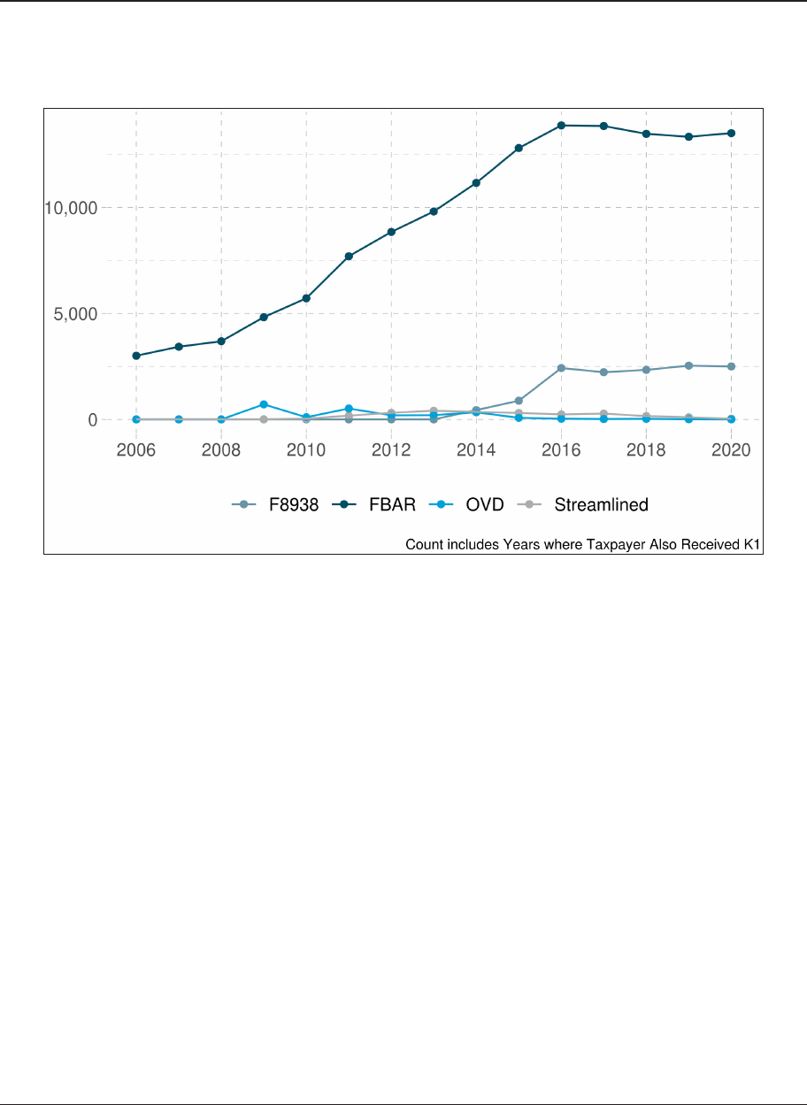
Wind, Bratt, Gra, and Herlache
FIGURE 1. Count of Taxpayers by Type of Foreign Account Reporting
e nal sample of taxpayers with foreign accounts was taken from individual taxpayers with a “signi-
cant stake” in at least one K- issuing entity from and . We dened “signicant stake” as directly
receiving percent
of the total absolute value reported by a payer. Figure shows the count of sample tax-
payers with foreign accounts and the years that they reported a foreign account and received a K-. We then
selected a sample of taxpayers for our comparison group. is group was made up of individual taxpayers that
have never reported holding a foreign account, were never reported to have a foreign account on Form ,
and were reported to hold a “signicant stake” in at least one K- issuing entity between and . Like
the foreign account holding sample, we also included the spouses of the nonforeign account holding sample.
At this stage, we had two groups of taxpayers that will make up our study population-taxpayers with re-
ported foreign accounts (RFA taxpayers) and taxpayers with no reported foreign accounts (non-RFA taxpay-
ers). We then get their K- network for every year that a taxpayer has received a K-. Specically, we created
nodes for all payers that issued K-s to RFA and non-RFA taxpayers, other payees that received a K- from the
same payer, and additional payers that issued K-s to the taxpayer’s neighbors. We repeated this process, for up
to ve levels from the initial taxpayer (see Figure ). Finally, we took one more step to clean the graph by re-
moving any nodes with over edges. With the foundation of each yearly graph set, we then added metadata
to each node from Form , as well as create multiple measures and descriptors of each taxpayer’s network.
Figure depicts an example of a ctional network, of an RFA taxpayer we’ll refer to as Node . Red edges
depict K- relationships, while green edges show spousal relationships. In a given year, Node received a K-
from Node A, which also issued a K- to Node . In addition, Node and Node received a K- from Node B.
Lastly, Node and Node were spouses in this year, but Node did not receive any K-s.
14
Note that the 30 percent signicant stake we require for a taxpayer to be included in the sample is distinct from the one percent threshold we set when building the
K-1 graph. We make the distinction because when building out a network we place a premium on having as complete a network as possible, taking into account
computational restraints; while when we select sample taxpayers, we prioritize ensuring that the taxpayer is an important part of the network.
15
More precisely, Node 4 did not receive any K-1s where it held at least a one percent stake.

Following K-1s: Considering Foreign Accounts in Context
FIGURE 2. Example Network in Graph
V. Graph Content
e nal sample contained , RFA taxpayers and , non-RFA taxpayers. Among the RFA taxpayers
in the sample, , taxpayers ( percent) reported a foreign account in only one year between and ,
while taxpayers ( percent) reported a foreign account in all een years. Taxpayers that report foreign
accounts in multiple years are more likely to report a foreign account in the years directly following the rst
disclosure. As shown in Figure , among RFA taxpayers that rst reported a foreign account between and
, percent also reported a foreign account ve years later.
FIGURE 3. Among RFA Taxpayers with First Foreign Account Between 2006-2015:
Percent with RFA in Years Following First RFA
Taxpayers with reported foreign accounts generally had higher reported income on Form . is was
true across all income types we included. As noted in Table , the median adjusted gross income (AGI) for

Wind, Bratt, Gra, and Herlache
RFA taxpayers in was around ,, while for non-RFA taxpayers it was around ,. e gures
presented in Table compare taxpayers who have ever reported a foreign account between and
with taxpayers who did not, not just in years where they reported a foreign account. is suggests the type of
taxpayers who reported foreign accounts and received K-s are dierent, at least in terms of reported income,
from K- recipients who never reported foreign accounts.
TABLE 1. Adjusted Gross Income by RFA Status, 2006–2020
Year
RFA Taxpayers Non-RFA Taxpayers
25th
Percentile
Median
75th
Percentile
25th
Percentile
Median
75th
Percentile
2006 $86,000 $213,000 $650,000 $39,000 $85,000 $172,000
2007 $91,000 $224,000 $679,000 $38,000 $86,000 $175,000
2008 $73,000 $192,000 $545,000 $34,000 $81,000 $162,000
2009 $61,000 $168,000 $459,000 $30,000 $75,000 $149,000
2010 $65,000 $182,000 $508,000 $33,000 $79,000 $156,000
2011 $68,000 $187,000 $526,000 $34,000 $82,000 $163,000
2012 $77,000 $208,000 $602,000 $38,000 $88,000 $177,000
2013 $78,000 $208,000 $556,000 $40,000 $92,000 $179,000
2014 $86,000 $221,000 $600,000 $42,000 $96,000 $194,000
2015 $84,000 $225,000 $604,000 $43,000 $99,000 $199,000
2016 $82,000 $222,000 $572,000 $44,000 $100,000 $201,000
2017 $87,000 $233,000 $614,000 $45,000 $104,000 $210,000
2018 $91,000 $238,000 $624,000 $47,000 $107,000 $220,000
2019 $92,000 $247,000 $629,000 $48,000 $111,000 $228,000
2020 $84,000 $240,000 $638,000 $46,000 $107,000 $228,000
Note: Due to condentiality concerns, all income amounts have been rounded to the nearest thousand dollars.
ere does not appear to be much evidence of a change in reporting behavior among RFA taxpayers aer
rst reporting a foreign account. In Figure , we look at RFA taxpayers who rst received a foreign account be-
tween and and received a K- for the six years surrounding the rst reported RFA to study whether
reported income changes in the years aer rst reporting a foreign account relative to the years before. We
then compared the results with non-RFA taxpayers to help ensure that any trends identied were not simply a
result of the passage of time. We randomly assigned all non-RFA taxpayers a value between and and
kept taxpayers with K-s in all three years before and aer that date. Panel A clearly shows the dierence in
median reported income and total tax among individuals who ever reported a foreign account and those that
did not. Panel B shows the percent change in each category relative to year zero (dened as the rst year with
an RFA for RFA taxpayers and the randomly assigned value for non-RFA individuals).

Following K-1s: Considering Foreign Accounts in Context
FIGURE 4. Reported Income for RFA and Non-RFA Taxpayers Over Time
In one nal look at reported income surrounding rst disclosing a foreign account, we focus in Figure
only on taxpayers who have at some point reported an oshore account. Here, we compared taxpayers who
have reported a foreign account in a specic year with those who did not report one. Figure A in the Appendix
shows once again that while there was some divergence between the two groups, it is not evident there was
a change in reporting behavior in the years surrounding when a foreign account was reported. We hope to
conduct a more rigorous statistical analysis to attempt to answer this question in future iterations of this work.
Similar to reported income, there does appear to be a dierence in the network structures between RFA
and non-RFA taxpayers. Networks of taxpayers who have ever reported a foreign account are larger both in
the number of taxpayers and dollars. e median network among RFA taxpayers contains taxpayers and has
reported , owing through the network, considerably larger than and , for non-RFA taxpay-
ers. As the median network size suggests, most K- networks contain only a handful of taxpayers. Around
percent of taxpayers who never reported foreign accounts contained fewer than four taxpayers. As is evident
in Figure , while the network of a plurality of RFA taxpayers also contained three or fewer taxpayers, RFA
taxpayers were far more likely to be in networks of over entities.

Wind, Bratt, Gra, and Herlache
FIGURE 5. Network Size by Whether Taxpayer Reported Foreign Account in a Given Year
VI. Modeling Approach and Results
While modeling directly from graphs is a growing area of research and would be worthy of exploration in this
context in the future, we opted to capture elements of the graph in a at le and. at that point, developed the
models we used in this paper. Converting the graph into a at le required creating numerous variables that
adequately represented the relationships and other insights evident in the graph. e variables created from
the graph and used for modelling were divided into three dierent categories: ) network variables; ) taxpayer
Schedule K- variables; and ) F reported income variables. Network variables included descriptions of
the taxpayer’s K- network including the composition and size of the network (e.g., number of taxpayers, per-
cent of network payers that are partnerships, multitiered pass-through entities as a percentage of network size)
and foreign account disclosure by network members (e.g., whether the network contains any RFA owners or
payers). Taxpayer K- variables directly described the relationship between the taxpayer and other members
of its network (e.g., number of K-s received, K-s received from multitiered pass-through entities as well as
from RFA taxpayers, the ratio of reported prots and losses on incoming Schedule K-s). Lastly, F vari-
ables captured amounts and types of income reported by the taxpayer on Form . For F values with
negative values, we took the absolute value, as taxpayers with large reported losses oen share characteristics
with taxpayers reporting large gains. In addition, due to the large range of income variables, we divided each
one into deciles of the absolute value of each income type. Deciles proved to be better predictors of reporting
a foreign account than the amount itself. A complete list of network variables used for modelling is provided
in Table A in the Appendix.
A primary objective of this work is to shed light on the relationship between a taxpayer’s network and their
likelihood to report a foreign account. To do this, we estimated a series of logistic regressions with individual
and year xed eects of the form:
y
it
=α+βx
it
+δ
t
+γ
i
+μ
it
,

Following K-1s: Considering Foreign Accounts in Context
where y
i t
is the likelihood of whether taxpayer reported a foreign account in time t. We rst estimated the
specication separately for each of the groups of covariates described above. erefore X is a vector of either
network, taxpayer Schedule K- or F variables for taxpayer i in time t, while β represents a series of coef-
cients for each individual covariates in x. e specication also includes year δ
t
and individual γ
i
xed ef-
fects. All continuous variables were scaled to allow for comparison across dierent coecients. Continuous
variables were scaled by rst subtracting the variable’s mean from each observation and then dividing by the
variable’s standard deviation. Finally, we combined all the covariate groups and estimated an additional regres-
sion of the form:
y
it
=α+β1net
it
+β2taxpayerk1
it
+β3f1040
it
+δ
t
+γ
it
+μ
it
–
-
able. For example, having a current RFA payer in their network, holding all other values constant, increase the
continuous variable.
We used the Akaike Information Criterion (AIC) to compare the goodness of t of the models. AIC takes
into account the likelihood of obtaining the observed data under the assumption that the model is correct,
while also penalizing a model for containing more variables to account for overtting. A lower AIC represents
a better tting model. Panel in Figure compares the AIC of the models specied. e model on the top row,
the taxpayer K- model, was the worst performing model using this metric. Of the models containing just one
group of variables, the F models performed best, with an AIC . percent lower than the taxpayer K-
model.

Wind, Bratt, Gra, and Herlache
FIGURE 6. Grouped Variables Regression Results
Panel 1: Network
Panel 2: Taxpayer K1
Panel 3: F1040 Panel 4: Combined
Panel 5: AIC Comparison
e combined model, which included all sets of variables is the best performing. While it may appear in-
tuitive that the specication that conveys the most information is the best performing, AIC takes into account

Following K-1s: Considering Foreign Accounts in Context
the model complexity and penalizes additional covariates. Nevertheless, the combined model’s AIC is per-
cent lower than the worst performing model. Table in the Appendix presents the results of the combined
regression. e analysis found that sharing a network with other taxpayers with reported foreign accounts is
positively associated with reporting a foreign account. is conrms our hypotheses that considering not only
a given taxpayer, but also the characteristics of their network is of informational value. is does not suggest
that individual attributes should be ignored. We nd that reporting higher income–(especially capital income)
and receiving income from a partnership (as opposed to an S-corporation and trust) are also positively associ-
ated with reporting a foreign account in that year.
VII. Future Work and Conclusion
is work demonstrates the value in considering a taxpayer’s K- network when assessing their likelihood
for noncompliance through failing to report a foreign account. We merely scratched the surface of analyses
that are possible by using a graph framework and other available taxpayer data in this space. For example, we
included a relatively small amount of variables from a limited set of categories. We did not include additional
taxpayer characteristics such as whether the taxpayer had a foreign address, whether they led an amended
return, country of foreign account, or their audit history. Moreover, other than a few notable exceptions (e.g.,
individual and year xed eects, looking at whether related taxpayers had previously had foreign accounts)
we did not fully exploit the time aspect of the data. On a related note, we took only a cursory look at how tax-
payer’s reporting behavior change aer rst reporting a foreign account; future work can dig deeper into this
question.
We faced various challenges when compiling the data. We faced data challenges that are inherent with
working with such a large and complex data set. To deal with some of these issues we trimmed the data by
introducing thresholds at various stages (described in more detail above). Subsetting the graph has two main
benets: rst, it allows us to focus on taxpayers that are more likely to be closely connected; and second,
working with multiple years of full K- data is computationally expensive. However, this approach does have
drawbacks such as arbitrarily attening the networks by limiting the number of payees and levels. is resulted
in less variation among the networks and may have biased our results towards representing network structure
and neighbor characteristics as less signicant than they actually are. Future work could experiment with con-
structing a graph that strikes a dierent balance between the trade-o between size and comprehensiveness.
We presented evidence that a relationship exists between a taxpayer’s K- network and reporting a foreign
account. Taxpayers with other payers and payees who report a foreign account are more likely to themselves
report holding a foreign account in that same year. While network and K- variables are associated with report-
ing foreign accounts, the model using only F variables is the best tting regression specied using only a
selection of variables. is, along with the results from the combined model, suggests that a combination of
taxpayer and network characteristics is necessary to gain an understanding of reporting foreign accounts. In
addition to exploring dierent taxpayer characteristics, future work can build on the framework we have laid
out and develop predictive models using machine learning methods such as random forests or graph neural
networks. In this work we lay a foundation for the work that is possible in this space and hope to continue to
develop methods to identify possibly noncompliant taxpayers and further aid in tax administration.

Wind, Bratt, Gra, and Herlache
Appendix
Figure A details income reporting behavior of reported foreign accounts (RFA) taxpayers that received a
Schedule K- for six consecutive years surrounding the rst reported RFA. We compared taxpayers who have
reported a foreign account in a specic year with those who did not (but did in another year).
FIGURE A1. Reported Income Among RFA Taxpayers by Whether Reported Foreign
Table A details the variables used in the dierent models. To address extreme values, we winsorized the
top . percent and (where applicable) the lowest . percent of F reported income to deal with extreme
values. In addition, we top-coded the absolute value of the K- dollar ows in the network to ,,,.
In both cases, these steps were taken before dividing the data into deciles.

Following K-1s: Considering Foreign Accounts in Context
TABLE A1. Variable Descriptions
Variable Description Category
Div Dec F1040 Decile of reported dividend income
Wage Dec F1040 Decile of wage income
AGI Dec F1040 Decile of the absolute value of adjusted gross income
Int Dec F1040 Decile of the absolute value of reported interest income
Capgain Dec F1040 Decile of the absolute value of capital gains income
Sch C Dec F1040 Decile of the absolute value of Sch. C income
Sch E Dec F1040 Decile of the absolute value of Sch. E income
Net Size Net K-1 Total number of unique entities in network
Per Parts Net Net K-1 Percent of network payers that issued 1065 Schedule K-1
Per Corps Net Net K-1 Percent of network payers that issued 1120s Schedule K-1
Per MPTE Net Net K-1 Pass-through entities as a percentage of the network size
Net Size Dols Dec Net K-1 The decile of the absolute value of the K-1 ows in the network.
Net Complex Net K-1 A network is complex if it contains a pass-through entity or a business
entity as a payee. A network is simple if all payers issued K-1s directly to
individuals.
Cur RFA Owner Net RFA Indicator whether there was an owner with a reported foreign account
in the network in the current year, excluding the taxpayer and his or her
spouse.
Pre RFA Owner Net RFA Indicator where there was an owner with a reported foreign account in a
previous year, excluding the taxpayer and his or her spouse.
Cur RFA Payer Net RFA Indicator whether there was a payer with a reported foreign account in the
network in the current year.
Pre RFA Payer Net RFA Indicator whether there was a payer with a reported foreign account in a
previous year.
K-1 from RFA RFA Indicator whether the taxpayer received a K-1 from a payer with a foreign
reported account in the current year.
Got F1065 Taxpayer K-1 Indicator whether the taxpayer received a 1065 Schedule K-1.
Got F1120 Taxpayer K-1 Indicator whether the taxpayer received a 1120s Schedule K-1.
Got F1041 Taxpayer K-1 Indicator whether the taxpayer received a 1041 Schedule K-1.
N K-1 In Taxpayer K-1 Number of K-1s received
Prot Loss Asym Taxpayer K-1 Sum of the absolute value of the dierence between the percentage alloca-
tion of prots and percentage allocation of losses.
K-1 from MPTE Taxpayer K-1 Indicator whether the taxpayer received a K-1 from a multitiered pass-
through entity.

Wind, Bratt, Gra, and Herlache
DEPENDENT variable: RFA in Year
Variable
Network Taxpayer K-1 F1040 Combined
(1)
(2)
(3)
(4)
Per MPTE Net
0.013
***
(0.001)
0.006
***
(0.001)
Net Size
0.012
***
(0.001)
0.002
***
(0.001)
Net Complex
-0.011
***
(0.002)
-0.003
(0.002)
Per Parts Net
0.002
**
(0.001)
0.004
***
(0.001)
Per Corps Net
-0.013
***
(0.001)
0.012
***
(0.002)
Net Size Dols Dec
0.026
***
(0.001)
-0.019
***
(0.001)
Cur RFA Owner Net
0.107
***
(0.003)
0.094
***
(0.003)
Cur RFA Payer Net
0.095
***
(0.003)
0.092
***
(0.003)
Pre RFA Owner Net
-0.023
***
(0.003)
-0.036
***
(0.003)
Pre RFA Payer Net
0.029
***
(0.004)
0.023
***
(0.003)
N K-1 In
0.015
***
(0.001)
-0.011
***
(0.001)
K-1 from MPTE
0.098
***
(0.002)
-0.004
**
(0.002)
K-1 from RFA
0.219
***
(0.004)
0.139
***
(0.004)
Prot Loss Asym
0.001
*
(0.001)
0.008
***
(0.001)
Got F1120
-0.002
(0.001)
-0.031
***
(0.002)
Got F1041
0.009
***
(0.002)
-0.030
***
(0.002)
Got F1065
0.075
***
(0.001)
0.017
***
(0.002)
AGI Dec
0.040
***
(0.001)
0.034
***
(0.001)
Int Dec
0.056
***
(0.001)
0.052
***
(0.001)
Div Dec
0.046
***
(0.001)
0.040
***
(0.001)
Wage Dec
0.002
***
(0.001)
0.003
***
(0.001)
Sch C Dec
0.006
***
(0.001)
0.003
***
(0.001)
Sch E Dec
0.001
(0.001)
0.005
***
(0.001)
Capgain Dec
-0.002
***
(0.001)
-0.004
***
(0.001)
AIC 783096.51 792926.51 757647.04 745516.38
Observations 704,857 704,857 704,857 704,857
R
2
0.050 0.036 0.084 0.099
Note: *p<0.1; **p<0.05; ***p<0.01.

Following K-1s: Considering Foreign Accounts in Context
Figure A shows the dierences between the networks of RFA and non-RFA taxpayers across dierent
dimensions. A higher percentage of taxpayers with foreign accounts received a K- from a pass-through entity
in a multitiered network, had another RFA owner or an RFA payer in its network.
FIGURE

Wind, Bratt, Gra, and Herlache
References
Agarwal, Ashish, Shannon Chen, and Lillian F Mills (2021). “Entity Structure and Taxes: An Analysis of
Embedded Pass-rough Entities.” e Accounting Review 96.6,1–27.
Agarwal, Ashish, Shannon Chen, Ririko Horvath, Larry May, and Rahul Tikekar (2015). “Analysis of Flow-
rough Entities Using Social Network Analysis Techniques.” IRS TPC Research Conference, Washington
D.C.
Black, Emily, Ryan Hess, Rebecca Lester, Jacob Goldin, Daniel E. Ho, Mansheej Paul, Annette Portz (2023).
“e Spiderweb of Partnership Tax Structures.” IRS Working Paper.
Cooper, Michael, John McClelland, James Pearce, Richard Prisinzano, Joseph Sullivan, Danny Yagan, Owen
Zidar, and Eric Zwick (2016). “Business in the United States: Who Owns It, and How Much Tax Do ey
Pay?” Tax Policy and the Economy 30.1,91–128.
Government Accountability Oce (2014). “Oshore Tax Evasion: IRS Has Collected Billions of Dollars, but
May be Missing Continued Evasion.” GAO Publication No.13-318.
Internal Revenue Service (2022). “Report of Foreign Bank and Financial Accounts (FBAR).”
https://www.irs.gov/businesses/small-businesses-self-employed/report-of-foreign-bank-and-financial-
accounts-ar.
Internal Revenue Service (2022). “Report of Foreign Bank & Financial Accounts (FBAR) Reference Guide.”
IRS Publication 5569.
Internal Revenue Service (n.d.). “Streamlined Filing Compliance Procedures–A Compliance
Option for Some Taxpayers” https://www.irsvideos.gov/business/FilingPayingTaxes/
StreamlinedFilingComplianceProceduresAComplianceOptionForSomeTaxpayers.
Internal Revenue Service (2022). “Summary of FATCA Reporting for U.S. Taxpayers.” https://www.irs.gov/
businesses/corporations/summary-of-fatca-reporting-for-us-taxpayers.
Internal Revenue Manual (IRM) § 4.63.3.1
Johannesen, Niels, Patrick Langetieg, Daniel Reck, Max Risch, Joel Slemrod (2019). “Taxing Hidden Wealth:
e Consequences of U.S. Enforcement Initiatives on Evasive Foreign Accounts.” NBER Working Paper
No.w24366.
Johannesen, Niels, Daniel Reck, Max Risch, Joel Slemrod, John Guyton, and Patrick Langetieg (2023). “e
Oshore World According to FATCA: New Evidence on the Foreign Wealth of U.S. Households.” NBER
Working Paper No.w31055.
Love, Michael (2021). “Where in the World Does Partnership Income Go? Evidence of a Growing Use of Tax
Havens.” Working Paper.
OECD (2013). “A Step Change in Tax Transparency.” OECD Report for the G8 Summit.
Olson, Matt, Annette Portz, Mike Feldman, Devika Mahoney-Nair (2022). “Graph-based machine learning
methods for case selection and population segmentation.” IRS Working Paper.

Application of Network Analysis To Identify
Likely Ghost Preparer Networks
Joshua W. King, Andrew J. Soto, Getaneh Yismaw, Izabel Doyle, Ririko Horvath, Ashley Nowicki,
Chris Hess
(IRS, Research, Applied Analytics & Statistics), Brandon Gleason (IRS, Criminal
Investigations), Will Sundstrom, Jacob Brooks, Michael Mastrangelo, Mike Stavrianos,
Daniel Hales (GCOM)
Introduction
More than half of individual taxpayers rely on paid tax return preparers to assist them in meeting their federal
tax ling obligations. In Filing Year , the IRS received ,, electronically led individual returns,
,, ( percent) of which were professionally prepared. Paid preparers are important IRS partners, as
the Service depends on them to help taxpayers comply with tax laws. Identifying noncompliant preparers or
groups of preparers who actively hide their identities, i.e., ghost preparers, is an essential component of the
IRS’s tax administration responsibilities. is paper describes ongoing eorts within the IRS to apply graph
techniques and network analysis to: () identify clusters of suspected ghost prepared returns; () understand
how ghost preparation unfolds during the ling season; and () study the impacts of ghost preparation on tax
compliance.
Ghost Preparer Risk
Ghost preparers represent a risk to the integrity of the U.S. tax system. By not identifying themselves on the re-
turns they prepare, they are not subject to oversight, and they are in violation of treasury rules and regulations.
In addition, ghost preparers may engage in abusive tax practices which harm taxpayers and undermine the
ecacy of the IRS. Compounding this concern, an individual ghost preparer may be responsible for tens if not
hundreds or thousands of returns, giving any fraudulent or abusive behavior an outsized impact. According
to the Treasury Inspector General for Tax Administration (TIGTA), ghost preparers disrupt and destabilize
established IRS practices, legitimate preparers, and the taxpayer ecosystem (TIGTA () and IRS ()).
Internal Revenue Manual (IRM) .... denes a ghost preparer as a compensated tax return preparer
who does not provide a Preparer Tax Identication Number (PTIN) on the returns they prepare as required
by Internal Revenue Code (IRC) section and Treasury Regulation .-. Ghost preparers may fail to
include any identifying number on prepared returns, or they provide a number other than a PTIN in place of
an appropriate PTIN, such as a series of random numbers, a Taxpayer Identication Number (TIN), a PTIN
issued to another preparer, a made-up PTIN, etc. A PTIN must be obtained by all return preparers who are
compensated for preparing or assisting with any U.S. federal tax return, refund claim, or other tax forms sub-
mitted to the IRS (unless specically exempted).
Ghost preparers may intentionally or unintentionally hide their identity. For preparers who are unaware
of the rules and requirements around PTINs, it is likely they are not qualied to provide advice and assistance
to their clients. ey may unknowingly put taxpayers at risk of not meeting their tax obligations and, in some
cases, audit by the IRS.
For preparers who knowingly hide their identity, there are many motivations to do so. Ghost preparers
may prey on taxpayers, stealing refunds or engaging in potentially illegal or fraudulent preparation strategies.
Even when the taxpayer is collaborating with the ghost to falsify returns to maximize refunds or claim un-
earned credits, the ghost preparer enables that illegal behavior. Ghost preparers may lie about their activities
to avoid their own tax liabilities or because they’ve already been identied as a problematic preparer and they

King et al.
are no longer allowed to prepare taxes. ere are unknown risks as well; ghost preparers are likely engaged in
schemes that have not yet been identied.
Innovation Lab
e Innovation Lab is an initiative at the IRS to encourage collaboration across the service on specic admin-
istrative or compliance challenges. In Fiscal Year the Innovation Lab sponsored research to apply network
analysis to detect and identify ghost preparers.
e objectives of the Innovation Lab were to explore multiple
network approaches to identify ghost prepared returns and to develop a tool for compliance sta to access and
investigate these networks for treatment. Ghost preparers are inherently dicult to identify because they do
not identify themselves on their clients returns. Many ghost preparers rely on do-it-yourself (DIY) soware
and not professional soware that is more tightly regulated. us returns completed by a ghost preparer
may look like individually led returns. Network analysis oers the promise of identifying related returns
from a ghost preparer by linking lings and revealing commonalities which point to a single preparer. Over
the course of Innovation Lab-sponsored research, analysts delivered a dataset of individual income tax returns
(Form ) networked across a range of ling and return characteristics for three ling years.
e lab delivered two network clustering approaches for grouping electronically led self-prepared Form
returns together into return clusters which may suggest ghost preparer involvement. Going forward,
those results should be updated with more recent data, additional data sources to build out the context of the
cluster networks, and for additional inputs to clustering approaches.
e lab produced a tool designed specically to deliver ghost preparer results to compliance and enforce-
ment sta. e tool includes features to prioritize and interrogate suspected ghost preparer return clusters to
connect analytical outputs with eld work.
Network Analysis
e concept of a network refers to “[an] object composed of elements and interactions or connections between
these elements” (Brandes ()). Calculations in a network model are referred to as network analysis or graph
analysis. Network analysis is useful in identifying interconnected groups of entities or clusters. Data stored in
a network model can reveal patterns or relationships that were not previously apparent.
Key concepts of a network model are nodes and edges. Entities are referred to as nodes and can encom-
pass wide range of things, depending on the application of that model. In the IRS context, nodes are generally
derived from tax forms. Relationships are referred to as edges. Edges connect pairs of nodes and represent the
relationship between them. Edges can contain information about the relationship between those two nodes
and may also convey information about the directionality of the relationship.
A key concept of network analysis is the idea of clusters. Clusters are groups of nodes that are connected
to each other within the network. Depending on the algorithm used or the structure of the network, clusters
can represent meaningful sub-networks of the larger network dataset. e structure of the cluster (the size and
distribution of nodes and edges) can convey information about which clusters are signicant. In addition, it
is possible to conduct calculations across the properties stored on nodes and edges to generate insights into
clusters.
Ghost Preparer Workow
e network analysis segment of the Ghost Preparer Project leveraged existing IRS data to reorient avail-
able tax return information into a network format to detect potentially ghost prepared returns. e modeling
conducted thus far follows a general process with three avenues for altering and targeting clustering results:
choosing data, establishing a network model, and applying clustering algorithms.
1
Currently, ghost preparer compliance treatments involve ad-hoc referrals or cases picked up in related compliance eorts. is research is an attempt to
systematically identify likely ghost preparer networks.

Application of Network Analysis To Identify Likely Ghost Preparer Networks
e process begins with identifying the datasets; the IRS maintains tax return information in a variety of
formats across a range of systems. In addition to return information, the network model can incorporate ad-
ditional datasets which the IRS maintains or has access to. Decisions regarding the data included in the model
have signicant eects on the modeling outcomes.
Once the data have been selected, the next step is to choose which elements to include in the network
model. Here decisions are made regarding what should be a node and what should represent relationships
between returns and what should be stored as a property. In addition, this provides an opportunity to limit ele-
ments added to the network model based on number of connections or other characteristics. It also provides
the opportunity for additional data manipulation, such as normalizing data elements.
e nal step and nal avenue for targeting results in the general workow is the application of the clus-
tering model. ere are several models available using a range of computing tools. Decisions about which
modeling tool to use can have signicant implications for the results generated, including whether results are
deterministic or probabilistic, as well as the average size of clustering results. Current analysis relies heavily on
the connected component algorithm, which is a deterministic clustering approach, and can be run against a
given network and returns all distinct subnetworks.
Benets of Network Analysis
Ghost preparation is characterized by complex networks of relationships between individuals involved; a net-
work model can capture these relationships. By analyzing the structure of the network, we can identify pat-
terns which suggest ghost preparation. In addition, data in a network format lends itself to seeing second and
third order connections between returns which facilitates connecting potential ghost preparers to the clusters
of returns identied.
Clustering Approaches
Approach 1. Risk-based
e Risk-based clustering approach scores returns and relationships to rene community detection algorithms
to return actionable clusters of returns with limited false positives. e Risk-based approach provides analysts
the ability to tune the analysis to focus on specic noncompliant behavior, suspicious behavior, and known
schemes undertaken by ghost preparers. By extension, it also controls for returns which would be addressed
using compliance programs outside ghost preparation, namely identity the (IDT). In addition to targeting,
the scoring removes spurious connections, which limits false positives or interconnected groupings of non-
compliant preparers.
Background
e Risk-based approach evolved from IDT detection eorts that grouped returns by submission character-
istics, which together are unique for most lers. Once grouped, the returns were assigned risk scores for a set
of IDT indicators, which allowed for ltering returns to a set of suspicious and inter-connected returns. From
this limited set of returns, additional related returns could be identied by considering a wider set of linking
factors. is approach eectively nds groups of returns that indicated IDT behavior and, unexpectedly, also
identied returns associated with ghost preparer behavior.
e Risk-based approach aims to address a series of challenges in interacting with networked returns
to detect ghost preparers. A pure networking approach would allow for links to be drawn from all specied
data elds within a tax return, but can create large unmanageable clusters, called super clusters. Super clusters
(e.g., clusters exceeding k returns) can be formed when spurious factors link several small clusters together,
or when return level data errors are present. Traditional networking algorithms alone can eectively identify
clusters within graphs, but the presence of a cluster does not necessarily imply ghost preparation. While com-
mon factors can be used to identify ghost preparers, they can also generate false positives.

King et al.
In the Risk-based approach, risk factors were identied from workstreams in IDT and from stakeholders.
Many of the risk factors are centered around the use of duplicate information from the tax return submitted
by the taxpayer/ghost preparer. In a group of properly self-prepared returns, a reasonably high degree of vari-
ability is expected, and it is suspicious for a large group of returns to share information. e more occurrences
of these shared factors, the riskier the return/group of returns is/are.
e Risk-based approach evolved from IDT detection eorts used during the Economic Impact Payments
stimulus program. e idea was to take returns and group them. Once grouped, risk scores could be assigned
for predetermined factors indicative of IDT or anomalous behavior. Once risk scores were assigned, the data
could be ltered to select the groups of returns with the highest scores. From there, a set of related returns
could be built. is yielded manageable cluster sizes and a manageable number of clusters that were indicative
of IDT behavior. An unexpected result of this approach was that it also showed returns with ghost preparer
behavior.
Mechanics
First Iteration: e approach began by selecting electronically led DIY returns and running them through
various steps to create a set of indicator variables. Indicator variables were binary and represented if the factor
was present or not present. Some factors were used to calculate an individual-level score, and that was used
in subsequent steps. Once indicator variables were created, they were grouped and scoring factors were cal-
culated. Most scoring factors were assigned scores based on the percent of that factor within a given group of
returns. Scoring was comprised of a score from -, with the higher the score the more present a factor is in
each grouping (Table ).
TABLE 1. Scoring Factors for Risk-Based Approach
Score Criteria Percent
0 Not present/not calculable
1 <26%
2 ≥ 26% and < 51%
3 ≥51% and < 76%
4 ≥76%
Once scores were assigned, groups of returns were selected using predetermined criteria. From there, the
groups were transformed back into return-level data and duplicates were removed. Post-transformation data
represented returns that were a part of groups that were considered suspicious based on return-level and
group-level characteristics. is data was the starting point for building networks of related returns.
Having selected an initial set of suspicious returns, the approached then iteratively added additional re-
turns with shared factors found in the suspicious set. is process was ve times to build a full set of returns
considered for the approach. With the full set of returns data was cleaned for formatting issues and known data
exclusions and then reformatted into a networked graph. From those networked results, distinct subnetworks
or clusters were identied using a connected components algorithm. Linking factors were determined based
on the potential for noise to be introduced into the results. More specic linking factors were chosen to elimi-
nate noise in the results and make for more manageable data and results representative of a ghost preparer.
Second Iteration: A second iteration of the Risk-based approach was created to improve community/
cluster scoring and better address super clusters. e rst step of the improved approach remains the same.
rough a series of steps, indicator variables were created that would later become part of the risk score and
were almost entirely the same as the indicators created for the rst iteration of the Risk-based approach with
additional focus on normalizing linking factors.
e updated approach builds a network using the normalized linking factors and generated clusters of
results using the connected components algorithm. Initial clusters of returns were assigned a cluster name,

Application of Network Analysis To Identify Likely Ghost Preparer Networks
and scores were calculated on risk factors using the same scoring method shown in Table . Returns were then
ltered using a predetermined set of thresholds. Communities of returns that met the scoring criteria agged
and recorded (rst run).
Returns from the rst run were queried and clusters that had a return count of more than set threshold
were separated. ese large groupings were restaged as a network and linking factors which were either highly
connected or had limited usage were removed. A second round of the community detection algorithm was run
against this limited network generating a nal set of clusters, with a limited number of super clusters.
Results
Results from the rst iteration of the Risk-based approach identied , clusters with a total of ,
returns. e average cluster size of the returns from the rst iteration of the Risk-based approach was .
when excluding the single super cluster, and . when including the super cluster.
Results from the second iteration of the Risk-based approach showed there were , clusters with a total
of ,, returns. e average cluster size of the returns from the second iteration of the Risk-based ap-
proach was ..
Approach 2. Top-down with Degree Limits
e Top-down approach is a network rst clustering approach. It relies on a connected components algorithm
to understand connections between tax returns. e IRS has used this strategy eectively in several tools and
contexts to nd groupings of tax returns. e approach is straightforward to apply and gives simply commu-
nicated information about likely groups of tax returns. is method enables the visualization and analysis of
the activity of ghost preparers by focusing on the direct correlations identied in the tax ling information.
Nevertheless, there are advantages and disadvantages to using connected components to look for connections
in tax lings, just like with any analytical tool. One advantage of this strategy over the Risk-based approach
is it does not assume ghost preparers engage in clearly risky behaviors. is allows analysts to discover ghost
preparers new and emerging schemes. It will also help identify preparers who create accurate returns but do
not sign them.
Background
e IRS has a long-established process for identifying ghost preparers and identity thieves by grouping returns
from tax return data. ese connections show patterns of actions or choices that a ghost preparer took when
preparing tax returns. is was primarily applied to smaller groupings of returns, generally limited by a geo-
graphic area or certain risk characteristics. e results were especially useful in identifying communities of tax
returns led by a specic ghost preparer and enabled analysts to identify key points of connection and target
interventions based on the possibility of fraud within the returns.
When this approach was applied to a less restricted set of returns, false positives and overlapping com-
munities became an issue, as well as massive unmanageable clusters or super clusters. Early attempts to nd
meaningful clusters using connected components dealt with this super cluster problem in a variety of ways.
One constructed the links but made no attempt to identify communities inside the super clusters. is enabled
analysts to manually visualize the relationships and detect clusters. e team decided that this was a starting
point for building clusters and learning about the connections between them.
Mechanics
is approach considers electronically led self-prepared tax returns. at data was reformatted to build a
network with normalized linking factors. Following the creation of the network, the connected components
technique was used to identify clusters based on a pre-determined set of linking factors deemed strong and
meaningful.

King et al.
Once the network was created, linking factors were removed based on their degree count. is network
analysis technique removes nodes from a network based on the number of connections they have; this limits
overly connected or infrequently used nodes.
Results
e connected components technique yielded a super cluster containing more than . million tax returns. It
also discovered , clusters of or more tax returns, containing a total of , tax returns. e number
of tax returns within the clusters ranged from to ,. Aer excluding the solitary super cluster, the average
cluster size was . tax returns. e , clusters must be examined further to identify false positives and
overlapping communities.
Approach 3. Label Propagation Algorithm
e previous two clustering approaches can both produce large super clusters of interconnected returns that
are not useful for analysis. While those approaches both try to avoid these super clusters, the binary nature of
edges in a graph (either present or not) means that they are inherently vulnerable to over connecting when
using noisy data. Label Propagation (LPA) is a network clustering algorithm that identies nodes which are
closely related. We use LPA on the ghost preparer project to break up those super clusters into smaller, more
meaningful, components.
Background
e over connection that leads to the formation of super clusters happens because we are using data elements
that contain noisy data. ese issues can aggregate together to create very large and connected components.
We can break up these large clusters into smaller components and remove some of the spurious connections
by using graph community detection algorithms, like LPA.
Since the over connected clusters can be the result of spurious connections, label propagation can remove
connections that are not supported by other nearby connections. e ability to break up over connected clus-
ters is important for two reasons. First, the networks in this process are generated in such a way that densely
connected areas are considered suspicious by default. is means that the large, over connected clusters oen
contain a disproportionate amount of ghost prepared returns compared to the rest of the clusters, so it is even
more important to be able to break them up. Second, the ability to break up these large clusters provides ex-
ibility creating networks.
With community detection algorithms, the only way that we can try to reduce the size and frequency of
these over connected clusters is to be more conservative when creating edges. is requires leaving out infor-
mation, or implementing complicated rules for creating edges will become hard to manage. Label propagation
gives us another avenue to address this problem so that we do not have to leave as much potentially valuable
information on the table.
Mechanics
Label Propagation works as follows:
1. Each node is given a unique label.
2. Each node changes its label to the most common label among its neighbors, with ties decided randomly.
3. Repeat Step 2 until no nodes change their label or you reach a predetermined number of iterations.
Label propagation has the eect of nding communities in the larger graph that have a high density of in-
ternal connections. e core idea is that once densely connected community settles on one label, there are not
enough connections to nodes outside of the community to change the labels of all the community members. In
the early stages, since all nodes are initialized with unique labels, there will be many tie votes that are decided
randomly. As the algorithm progresses and communities start to form, there are fewer and fewer ties, and so
there are fewer randomly decided winners.

Application of Network Analysis To Identify Likely Ghost Preparer Networks
Results
Label Propagation was used to break up the super cluster of almost million returns that was created dur-
ing the Top-down clustering process. e initial cluster of ,, returns was broken down into ,
smaller clusters, ranging in size from return to , returns. e mean cluster size was . returns, and the
th
,
th
, and
th
percentiles for cluster size were , , and returns, respectively.
Other Topics
Ghost Preparer Tool
From the initial planning phases of the Innovation Lab, the team emphasized the importance of operational-
izing any ghost preparer analysis results. To facilitate this, the planning team requested and received funding to
develop a ghost preparer specic tool. In January , the innovation lab released a beta of the Ghost Preparer
Tool (GPT). e tool is designed to identify potential cases and investigate networks of returns for ghost
preparers. From a data perspective the tool consists of two main components: a multi-year dataset of e-le
Form returns stored in a network format and clustering results. e tool was designed to take advantage
of existing graph tools within the IRS and to be as exible as possible to accommodate new data sources and
clustering techniques as they become available.
Work Streams
e tool is designed to support two workstreams, the rst of which is case discovery. e aim is to allow users
to review clusters of self-prepared returns to detect previously unidentied schemes or cases. A key piece of
this work stream is standard cluster metrics generated for all clusters that have been added to the tool. e tool
allows users to specify thresholds and lter and order lists of clusters based on cluster metrics irrespective of
clustering technique. Users can download lists of suspicious clusters or use the tool’s interface to explore the
clusters of returns they’ve selected. e tool also includes a feature set where users can add notes to clusters
allowing for deconiction and collaboration between users.
e second workstream is the investigation of suspicious groupings of returns. ere are two features in
the tool which support this workstream: a full text search engine and graph visualizations. Full text search
enables users to quickly search a point of connection across the entire reference dataset to if they have al-
ready been identied as being part of a cluster and to quickly see all returns related. e second component
of the tool which supports the investigative work stream is the graph visualization of clusters. Here, users can
graphicly explore the connections which exist between returns as well as reports generated for clusters. Users
also have the ability run a set of predened and user dened graph traversals to reveal potential leads.
Graph Neural Networks
Background
Graph Neural Networks (GNNs) are a variation of standard neural networks that use connections between
data to perform machine learning tasks. is connection data can be used in addition to standard tabular data,
but it could also be used on its own, if the focus of the machine learning task is to learn about the graph struc-
ture. ere are dierent types of GNN models, but one of the common types of GNN, convolutional neural
networks (CNNs), takes inspiration from approaches that were developed for computer vision tasks.
CNNs use a convolution layer that has the eect of sweeping a small window across an image. ese
smaller, windowed image segments are then what the neural network is trained to recognize, and this ap-
proach provides several benets. By moving a small window across the image, the model is trained to pick out
smaller scale details like the borders between objects or facial features, ignoring their placement in the overall
image. In other words, this sliding window focuses the learning eorts of the model on the local structure of
the image as opposed to the global structure. is approach also makes the model better at generalizing to
images of dierent sizes and shapes.

King et al.
Graph Convolutional Networks (GCNs) are GNNs that take inspiration from CNNs. GCNs focus learn-
ing on small scale graph structures instead of whole graphs and are better able to handle graphs of dierent
scales. One of the most interesting things about GCNs is that they are generally very ecient to implement,
both in terms of data preprocessing and in terms of actual computation. Standard CNNs include extra hy-
perparameters and choices to be made about the convolution process. GCNs, on the other hand, can leverage
the deep connections between graph theory and linear algebra so that they are relatively simple to create and
computationally ecient.
Application to Ghost Preparers
GNNs can help when we are in a situation where the data must be evaluated in context. e returns prepared
by ghosts are usually prepared with the cooperation of the ler, and so in isolation there may be few or no in-
dications that the person who prepared this return was not the person who led it. Ghost preparers are usually
discovered because a group of returns that have been signed by dierent DIY lers all have some indication
that they may actually have been prepared by one actor.
GCNs address this problem because they can take the values of features of neighboring nodes into account
when creating vector representations (embeddings) of either nodes, edges or entire graphs. ese embeddings
can then be used for dierent downstream tasks, like classifying nodes, classifying graphs, predicting links, or
detecting anomalies.
Current Plans
e ghost preparer team is currently working on a prototype GCN model. is initial model will be a link pre-
diction model, with the goal of learning how preparers are linked to returns that they prepare so that we them
predict links between ghost prepared clusters and who may be preparing those returns. One of the benets of
this research is that once there is a process in place to create meaningful embeddings of the data with the GCN,
it is relatively simple to then apply those embeddings to dierent downstream tasks. Depending on how our
link prediction experiment goes, we can explore unsupervised anomaly detection for nding potential ghost
prep clusters and can also test out supervised models once we accumulate enough data on conrmed ghost
preparers to use as labels.
Future Analysis
Cluster Timelines
Using network-based approaches to detect ghost preparers requires the suspect network to be mature enough
that we can detect signs of ghost preparing behavior. Networks are considered fully formed at the end of the
tax season and returns that would be present in any given cluster are present in the network. However, the
end of the tax season may be post-refund and more cumbersome to deal with from a compliance standpoint.
A cluster timeline analysis was completed to look at various snapshots throughout the tax season to see if
Document Locator Numbers (DLNs) identied through the Risk-based approach would appear at the end of
the tax season in a suspicious cluster of or more returns.
Approach
e Risk-based approach was run using all the data available for ling season . e dataset containing
the selections of possible ghost preparers served as the comparison group and is referred to as the nal set.
e Risk-based approach was run again at three dierent times during ling season : February (Group
Timepoint (T)), March (Group Timepoint (T)), and April (Group Timepoint (T)). e approach was
run in its entirety, and the approach remained the same for all the time points as it did for the nal set, except
that the cluster size minimums for groups T to T were dropped down from returns to returns. Results
from groups T to T were transformed into cluster-level data. Returns were grouped by cluster size and the
number of clusters that have that given cluster size were recorded (e.g., in cluster size , there were , clus-
ters that had that given cluster size; see Table ).

Application of Network Analysis To Identify Likely Ghost Preparer Networks
Additionally, the DLN count was computed for each cluster group size (e.g., there were , returns
that were a part of a cluster group size ). From there, four data points were computed for each given cluster
group size: the number of suspicions DLNs (returns) that appeared in the nal set; the percentage of DLNs
that appeared in the nal set; the percentage of the clusters where % of the returns appear in the nal set
(Percent of % Clusters in Final Set); and the number of clusters, where all of the returns appear in the nal
set (Number of % Clusters in Final Set).
TABLE 2. Timepoint Snapshot Example, February 2021
Group Group Size
Total
Clusters
Percent of
Clusters
Total DLNs
Suspicious
DLNs
% of DLNs
in Final
# of 100%
Clusters in
Final Set
T1 6 10,435 7.06 62,610 4,493 7.18 737
T1
7 5,688 9.53 39,816 3,893 9.78 542
T1
8 3,687 13.48 29,496 4,063 13.77 497
T1
9 2,459 17.97 22,131 4,105 18.55 442
T1
10 1,900 21.53 19,000 4,254 22.39 409
Cluster-level data were further transformed into cumulative data for each group (T to T), and the cluster
group sizes were collapsed into groups of plus, plus, plus, plus, and plus (e.g., plus represented
cluster group sizes of or greater). For each transformed group, suspicious returns (DLNs), total returns
(DLNs), DLN percentage in nal set, and cluster percent in nal set were calculated. e idea was to create
groups of returns with realistic cuto criteria but with no specic grouping size selected. Instead, it is more
likely and more logical to say that cluster group sizes of plus have more suspicious returns than cluster
group sizes that have exactly returns.
Results
Timepoint . Results showed that the Risk-based approach identied suspicious DLNs in T (February snap-
shot) among all groups of cumulative cluster sizes better than chance ( percent). In T . percent of DLNs
showed up in the nal set for cluster sizes of or greater (see Figure ). is percentage increased to .
percent for clusters of or greater and . percent for clusters or greater (see Figure ). Percentage de-
creased for cluster sizes of or greater (. percent) and or greater (. percent).
Timepoint . Results showed a similar pattern of increasing percentage as cumulative group size increased
in T (March snapshot), but it began at a lower percentage than timepoint (T). For cluster group sizes of
plus, . percent of DLNs appeared in the nal set (see Figure ). Percentages increased in cluster group
sizes of plus (. percent), cluster group sizes of plus (. percent), and cluster group sizes of plus
(. percent). For cluster group sizes of plus the percentage decreased to . percent.
Timepoint . A similar pattern of increasing percentage was seen in T (April snapshot), and like T the start-
ing percentage began lower than percent. For cluster group sizes of plus, . percent of DLNs appeared
in the nal set and increased to . percent for cluster group sizes of plus (see Figure ). Percentages
continue to increase for cluster group sizes of plus (. percent), and cluster group sizes of plus (.
percent). Lastly, percentages decreased down to . percent for cluster group sizes of plus.

King et al.
FIGURE 1. Detection of Suspicious Ghost Preparer Clusters for Three Time Points
Results from the Cluster Timeline Analysis supported the idea that the Risk-based approach can detect
suspicious returns at various timepoints in the tax season, and those same suspicious returns are likely to show
up at the end of the tax season in a suspicious cluster of or more returns. However, the Risk-based approach
uses a predetermined set of scores to identify clusters of returns as suspicious, and it is possible that over time
with various schemes those markers would evolve or become extinct. Additionally, the Risk-based approach
uses degree ltering to break up large clusters, and it is possible that in earlier snapshots returns were in small
cluster and identied as suspicious. In later snapshots, those returns could have fallen into a super cluster and
have been broken into a smaller cluster that was not suspicious. Lastly, the approach does not track returns
over time, as it is not looking at the same cluster and how it changes. Instead, the analysis represents three dis-
tinct snapshots and shows the percentage of DLNs that show up in the nal set. e simplicity of the Cluster
Timeline Analysis allows it to be implemented for any other networking approaches being used to identify
ghost preparer networks.
Impact Analysis
e aim of this analysis is to leverage the clustering results generated during the Innovation Lab analysis and
subsequent modeling to provide insight into the risks ghost preparers may pose to the fair and eective imple-
mentation of the U.S. tax code. To measure that risk, this analysis focuses on how returns changed from tax
year to tax year for individuals who appear to transition to ling with a ghost preparer. is work can help us
to begin to understand the potential impact ghost preparers have on a return-by-return basis and, in the fu-
ture, can be extrapolated to provide a picture of the impact ghost preparers have in the aggregate. is analysis
compares changes across return characteristics and established risk metrics.
Anecdotal evidence backed by analysis of the clusters identied during the Ghost Preparer Innovation
lab suggests that ghost preparers do not work with a group of taxpayers that is representative of the entire
taxpaying population. Ghost prepared clusters tend to be lower income lers, but there are indications that
there may be other communities which disproportionately see ghost preparer involvement. At this point in
our understanding of ghost preparers, keeping the analysis limited to individuals who appear to have worked
with a ghost preparer limits the risks of attributing the ling behavior of a specic community or demographic
to ghost preparers.

Application of Network Analysis To Identify Likely Ghost Preparer Networks
Approach
We considered clustering results generated using the risk-based clustering for Tax Years (TYs) , , and
. From those clustering results we selected a sample of , primary lers and considered their returns
for the three tax years used in clustering. From that dataset we identied two groups of returns, those where
the ler transitioned into a cluster and those where a ler stayed in a cluster. Conceptually we considered these
two groups—joined ghost preparer and stayed with a ghost preparer. For the two groups, we compared year-
over-year changes in their returns to attempt to understand the eect joining a suspicious cluster has on their
lings.
When a primary ler led a return the previous tax year that wasn’t identied with a cluster and then les
a return in the current year that is identied with one, we determined that the ler joined a ghost preparer.
When a primary ler led returns identied with a cluster in consecutive tax years, we determined that the
ler stayed with a ghost preparer. Cases when the primary ler did not le in the previous year, transitioned
out of a cluster, or remained outside of a cluster in consecutive years were excluded from consideration.
For TYs and of the , primary lers we considered, we found , returns where the ler
joined a ghost preparer and , where the ler stayed with a ghost preparer. For these groups of returns, we
measured year-over-year changes as the dierence in values.
Limitations and Assumptions
ere are several assumptions and limitations in the analysis. As stated elsewhere, we do not have labeled
data, so we assume that the clusters of interconnected self-prepared returns we detect represent individual
ghost preparers and that all returns in each cluster are ghost prepared. We recognize that there may be false
associations, returns incorrectly identied as being ghost prepared, as well as returns where we do not detect
the involvement of a sophisticated ghost preparer. We do not currently have a measure of the extent to which
we misidentify ghost preparers.
is analysis hinges on the intuition that ghost preparers engage in consistent behavior year over year and
that they treat new and returning clients to their illegitimate practice the same. An extension of that assump-
tion is that where a ghost preparer adopts a new scheme or preparing practice, we assume it is generally em-
ployed across all returns they prepare. It is worth recognizing if a ghost preparer treats new patrons dierently
or if they prepare randomly, it could add a confounding variable to our analysis.
e second key assumption is that the changes in the returns of individuals we’ve identied as transition-
ing to ghost preparers are due to the ghost preparer rather than the motivation for the individual to seek out a
ghost preparer. It is conceivable that individuals choosing to prepare with a ghost preparer may do so due to a
change in their tax situation. It is dicult to statistically disambiguate victims of a ghost preparer and taxpay-
ers working in collaboration with their preparer.
A nal important consideration for this analysis is that it spanned the COVID- pandemic. is is a peri-
od of change in employment and earnings for many Americans, which had the potential to impact the results.
Return Distributions
When considering year-over-year changes, initial ndings supported the assertion that ghost preparers do
inuence their clients’ returns. Individuals joining a suspected ghost cluster in comparison to individuals
remaining in a ghost cluster are more likely to see changes in their return characteristics from tax year to tax
year. In addition, preliminary results showed that rst year clients and returning clients are comparable across
income and credits claimed suggesting that we are comparing a similar population of lers.
e most notable change from the perspective of tax administration was refunds. Risk-based cluster re-
turns that transitioned to a ghost preparer saw a increase in average refunds for TYs and com-
bined, compared to returning ghost preparer cluster lers. Average annual increases in refunds were paired
with increases in average reported incomes and withholding, which, while notable, did not provide a clear
picture of noncompliance.
King et al.
TABLE 3. Comparative Annual Changes in Reported Income and Refunds
Return
Element
Tax Period
Average Value on F1040 Annual Change Annual % Change
Joined GPC Stayed GPC Joined GPC Stayed GPC Joined GPC Stayed GPC
Total Income
TY 2020 $43,154 $39,721 $6,853 $1,268 16% 3%
TY 2021 $39,061 $42,941 $2,572 $745 7% 2%
Total $40,937 $41,337 $4,538 $1,005 11% 2%
Adjusted Gross
Income
TY 2020 $42,594 $39,122 $6,880 $1,232 16% 3%
TY 2021 $38,395 $42,413 $2,370 $851 6% 2%
Total $40,320 $40,774 $4,442 $1,040 11% 3%
W2 Wages
TY 2020 $39,331 $40,244 $2,220 -$388 6% -1%
TY 2021 $41,900 $45,075 $3,140 $3,530 7% 8%
Total $40,706 $42,648 $2,717 $1,579 7% 4%
Total Tax
Amount
TY 2020 $3,786 $2,210 $1,125 $24 30% 1%
TY 2021 $2,922 $3,138 $555 $353 19% 11%
Total $3,301 $2,687 $817 $189 25% 7%
Withholding
Amount
TY 2020 $3,932 $3,891 $599 -$17 15% 0%
TY 2021 $3,876 $4,384 $169 $411 4% 9%
Total $3,902 $4,138 $367 $198 9% 5%
Refund Amount
TY 2020 $3,744 $4,194 $508 -$43 14% -1%
TY 2021 $4,755 $4,394 $1,042 $170 22% 4%
Total $4,291 $4,294 $797 $64 19% 1%
Earned Income
Credit
TY 2020 $2,843 $2,994 -$49 -$188 -2% -6%
TY 2021 $2,621 $2,775 $185 $29 7% 1%
Total $2,712 $2,884 $78 -$79 3% -3%
An additional nding of note is that there was no major year-over-year change in Earned Income Tax
Credit (EITC); neither the rates at which it is claimed, nor the average value of the credit. is is signicant
because it showed changes in refunds do not appear to be driven by the EIC and that, for this clustering ap-
proach, transitioning to a ghost preparer doesn’t appear to have a major change in EITC behavior of taxpayers.
TABLE 4. Year-Over-Year Change in EITC Claims
Dropped No Change Added Net Change Percent Change
Tax Year 2020
Joined GPC - 38 807 + 43 5 1%
Stayed GPC - 53 889 + 32 -21 -2%
Tax Year 2021
Joined GPC - 32 965 + 48 16 2%
Stayed GPC - 48 907 + 27 -21 -2%
Totals
Joined GPC - 70 1772 + 91 21 1%
Stayed GPC - 101 1796 + 59 -42 -2%

Application of Network Analysis To Identify Likely Ghost Preparer Networks
We do observe lers joining suspicious clusters show higher year-over-year changes in Schedule C usage.
is could indicate that ghost prepares are fabricating business income and losses to maximize refunds for
their clients however this analysis doesn’t provide evidence of noncompliance.
TABLE 5. Year-Over-Year Change in Schedule C Usage
Dropped No Change Added Net Change Percent Change
Tax Year 2020
Joined GPC - 53 740 + 95 42 5%
Stayed GPC - 67 856 + 51 -16 -2%
Tax Year 2021
Joined GPC - 37 858 + 150 113 11%
Stayed GPC - 40 879 + 63 23 2%
Totals
Joined GPC - 90 1,598 + 245 155 8%
Stayed GPC - 107 1,735 + 114 7 0%
Discriminant Function Score Distributions of Cluster Returns
In looking for ghost preparer eects we consider an existing IRS risk metric, the discriminant function (DIF)
score, to provide insight into the compliance risks posed by clusters of interconnected self-prepared re-
turns. e DIF scoring algorithm is a technique that has been used since to predict how likely a tax return
is to have a signicant adjustment. Individual and small corporation income tax returns, and S corporation,
and partnership tax returns receive a DIF score during processing. e score is calculated and stored in the
administrative data system, then is used in downstream systems during examination selection.
DIF encompasses a series of models that are specic to mutually exclusive tax classes known as activity
codes. Returns are assigned an activity code based on total positive income, total gross receipts, and EITC.
ese classes help in guaranteeing fairness by providing balanced coverage for all tax return types. By develop-
ing a model for each activity code, similar returns can be compared to one another, enabling more accurate
predictions about the population, and allowing for the most noncompliant returns to be selected. A high DIF
score indicates that the return has a high likelihood for signicant tax change overall and that auditing that
return will lead to a tax change. DIF score distributions are not consistent across activity codes or processing
years, meaning models cannot be compared to one another.
To allow for comparison year to year across all ling types we consider returns which fall within the top
percent of DIF scores, indicating they’re the riskiest returns irrespective of processing year or activity code.
Results. For the two tax years considered, and , we found that on net, percent of returns where
the ler joined a ghost cluster moved into to the
th
percentile of the DIF distribution from the previous tax
year compared to percent of returns where the primary ler stayed with a ghost preparer. ese results are
not conclusive, but they do indicate that ghost preparers do not lessen the audit risk to the taxpayer or improve
compliance on average.
Overall, however, we found all returns in the population considered to be signicantly more likely to fall
in the top percent of the DIF distribution. Returns in suspected clusters, both rst time and repeat lers, fell
within the top percent of the DIF distribution at rates of percent and percent respectively across TYs
and , indicating they are more than times as risky as returns overall when considered from a DIF
perspective. For TY , our sample includes , lers who self-prepared and would go on to be identied
in a suspected ghost cluster in TY , for that group of the returns, or percent fell within the top
percent of the DIF distribution. While not as high as the returns identied in ghost clusters for the same year,
( percent) it still is much higher than we would anticipate.

King et al.
TABLE 6. Returns in the 95th Percentile of the DIF Distribution
Total
Returns
Returns in 95% of DIF
Distribution*
Left 95%
No
Change
Joined 95%
Net
Change
Tax Year 2020
Joined GPC 888 14% -52 772 +64 +12
Stayed GPC 974 16% -61 849 +64 +3
Tax Year 2021
Joined GPC 1,045 18% -59 878 +108 +49
Stayed GPC 982 18% -67 832 +83 +16
Totals
Joined GPC 1,933 16% -111 1,651 +172 +61
Stayed GPC 1,956 17% -128 1,681 +147 +19
* This value is 5 percent in the population overall.
Next Steps
Validate
An important next step for the larger project and for this analysis is to measure the eectiveness of the vari-
ous clustering approaches. Validation generates feedback which can improve existing processes and provides
important context to the analysis results. ere may be options to use existing IRS data or processes for this
purpose, but each has its own challenges and limitations. One possibility would be to use compliance and
enforcement data to check if previously identied ghost preparers would have been identied using network
analysis. Another approach might be to use IDT identication detection processes to identify overlap with
ghost preparation results. ere may be additional options as well.
Validation can help to identify potential biases or gaps in clustering results which is critical to this eort.
False positives could have serious consequences for taxpayers who legitimately self-prepare their returns as
well as individuals falsely identied as ghost preparing returns. In addition to limiting risk to the taxpayer,
verifying results can highlight failures of the model to identify known ghost prepared returns which may rep-
resent gaps in enforcement. Ghost preparer patterns and approaches likely evolve overtime, generating labeled
data is key to improving models and staying ahead of new schemes.
When a ghost preparer is detected, the IRS does undertake outreach and compliance actions to help that
preparer meet their legal obligation. In some cases, the IRS may pursue a criminal investigation of the pre-
parer. As a result, the IRS does have information about known ghost preparers. One approach for validating
clustering results would be to check if they detect known ghosts.
ere are challenges in doing this as well as some limitations to how generalizable we could expect the
results. Compliance datasets are primarily oriented around the ghost preparer, while the cluster analysis is ori-
ented around returns. e complicates analysis because it requires dealing both with the uncertainty around
the ghost and their clientele, for a known ghost we may not have an exhaustive picture of the returns they
prepared and for the suspected returns we may not have a full picture of the ghost preparer. Creating a cross
walk between the two will be a challenge.
A limitation, which may be abating, is the delay between detection and action. Investigations and pros-
ecutions may take years, so many denitively identied ghosts were not active during the processing years for
which the clustering results are available. is means that known ghosts, either prosecuted or treated and the
returns identied using network analysis have limited overlap. Finally, ghosts the IRS has detected and treated
may not be representative of ghost preparers overall, so looking at these datasets may not provide a true picture
of the eectiveness of the clustering.

Application of Network Analysis To Identify Likely Ghost Preparer Networks
e IRS does commit resources to detecting IDT in real time to limit risk of individuals being unable to
le returns and reduce the harm to the government. Some of these processes may also identify ghost preparers
in real time. One option would be to collaborate with the IDT detection teams to look for overlaps. e major
limitation of this approach is that while it may corroborate the current approaches, it is not denitive.
Ghost Preparer Compliance Study
By leveraging important insights learned thus far using the GPT network analysis techniques that identify
suspected ghost preparers, a compliance study program could be established to enable the Service to study
ghost preparers’ compliance behaviors and eects on tax administration. A potential ghost preparer compli-
ance study might involve examining a portion of tax returns they prepared to assess compliance changes. e
study should consider elements such as income underreporting and credit overclaims which would require a
two-step sampling design.
A formal compliance study, if undertaken, should involve various stakeholders to set priority goals and
determine the size of the study needed based on available resources and additional data to be captured, among
many factors. Since there is no ghost preparer audit data, what follows is a possible starting point.
Objectives of Ghost Preparer Compliance Study
1. Estimate ghost preparer population and related characteristics,
2. Estimate impact of ghost preparers on tax compliance and tax-administration, and
3. Use result of the study to enhance ghost preparer compliance strategy.
First-Stage Sample. Select a random sample of clusters (networks) from a population of suspected ghost
preparer networks
identied by the two clustering approaches: Risk-based and Top-down. Provisionally, this
can be done by selecting equal number of rst-stage samples of suspected clusters from each clustering ap-
proach. Since suspected ghost preparer clusters range by sizes of returns, stratication of the rst-stage sample
by network size will be an appropriate approach to make sure some of the large volume clusters are included.
Second-Stage Sample. For each of the rst-stage samples of suspected ghost preparer networks selected,
select a random sample of returns (customers of suspected ghost preparers) with an explicit objective of posi-
tively identifying the suspected ghost preparer
and assess the nature and level of noncompliance at the return
level. e second-stage sample size for each rst-stage sample cluster will depend on resources, but a starting
point could be proportional-to-size, with the minimum number of returns (customers) necessary to positively
identify the ghost preparer, as determined by subject matter experts.
While a formal ghost preparer study can be implemented as part of existing compliance programs, there
will be extra eorts and data capturing needs that will require additional resources. However, the long-term
benet of the outcome data of the study will far outweigh the initial costs. In addition to being able to have
a reasonable impact estimate with a Ghost Preparer Compliance outcome data, a more tailored compliance
strategy and treatment option(s) can be established by developing supervised predictive machine learning
algorithms, such as GNN, that can better identify potential ghost preparers. Without outcome data, the best
modeling eort that can be done at this point is some sort of unsupervised anomaly detection method whose
eectiveness and reliability cannot be as easily assessed during modeling. Furthermore, with outcome data, the
eectiveness of the networking approaches can be valuated and improved, iteratively.
2
a big step up from current practices, the level of inference that can be made using this compliance data will be limited.
3
For each rst stage sample cluster, we would need a second stage sample size of returns audited to positively identify the ghost preparer and to produce compliance
level at a network level.
4
If results from the Ghost Preparer pilot treatment options are available, a formal model-based sampling design can be constructed.

King et al.
References
Brandes, Ulrik (2005). “Network Analysis: Methodological Foundations.” Volume 3418. Germany: Springer
Science & Business Media.
Internal Revenue Service (IRS) (2009). “Publication 4832, Return Preparer Review, Rev. Dec. 2009
TIGTA (July 25, 2018). “e Internal Revenue Service Lacks a Coordinated Strategy to Address Unregulated
Return Preparer Misconduct.” Treasury Inspector General for Tax Administration Ref. No. 2018-30-042

5
∇
Appendix
Conference Program

Conference Program
13th Annual IRS-TPC Joint Research Conference on Tax Administration
June 22, 2023
Program
:–: Opening
Wendy Edelberg (Director of the Hamilton Project, Brookings Institution)
Eric Toder (Co-Director, Urban-Brookings Tax Policy Center) and
Barry Johnson (Deputy Chief Data and Analytics Ocer, Research, Applied Analytics
and Statistics (IRS)
:–: Session : Service is Our Surname
Moderator: Deena Ackerman (U.S. Department of e Treasury)
» Looking Beyond Level of Service: Using Behavioral Insights to Improve Taxpayer
Experience
Jan Millard (IRS, RAAS); Sarah Smolenski, Jonah Flateman, Jamil Mirabito, Omar
Faruqi, Lauren Szczerbinski, Michael Stavrianos (ASR Analytics)
» e Balance Due Taxpayer: How Do We Reduce IRS Cost and Taxpayer Burden for
Resolving Balance Due Accounts?
Howard Rasey, Shannon Murphy, Frank Greco, Javier Framinan (IRS, W&I); Angela
Colona, Javier Alvarez (IRS, Taxpayer Experience Oce)
» Understanding Yearly Changes in Family Structure and Income and eir Impact on
Tax Credits: Can Tax Credits Be Advanced?
Elaine Maag, Nikhita Airi, Lillian Hunter (Urban-Brookings Tax Policy Center)
» Racial Disparities in Audit Rates
omas Hertz (IRS, RAAS)
Discussant: Janet Holtzblatt* (Urban-Brookings Tax Policy Center)
Emily Y. Lin* (U.S. Department of the Treasury)
:–: p.m. – Break
:–: p.m. – Session : Estimating Audit Aershocks
Moderator: John Guyton (IRS, RAAS)
» Changes to Voluntary Compliance Following Random Taxpayer Audits
Allan Partington, Murat Besnek (Australian Taxation Oce)
» e Long-Term Impact of Audits on Nonling Taxpayers
India Lindsay, Jess Grana (MITRE); Alan Plumley (IRS, RAAS)
» Silver Lining: Estimating the Compliance Response to Declining Audit Coverage
Alan Plumley, Daniel Rodriguez (IRS, RAAS); Jess Grana, Alexander McGlothlin
(MITRE)
Discussant: William Boning (U.S. Department of the Treasury)

Conference Program
:–: p.m. – Keynote Speaker/Lunch
Catherine Rampell (Washington Post)
:–: p.m. – Session : Understanding Contemporary Taxpayers
Moderator: Russell James (IRS, RAAS)
» Who are Married-Filing-Separately Filers and Why Should We Care?
Emily Y. Lin, Navodhya Samarakoon (U.S. Department of the Treasury)
» Willing but Unable to Pay? e Role of Gender in Tax Compliance
Andrea Lopez-Luzuriaga (Universidad del Rosario); Carlos Scartascini* (Inter-American
Development Bank)
» Who Sells Cryptocurrency?
Jerey L. Hoopes (University of North Carolina at Chapel Hill); Tyler S. Menzer, Jaron
H.Wilde (University of Iowa)
Discussant: Yan Sun (IRS, RAAS)
: p.m. - : p.m. – Break
:–: p.m. – Session : Hidden Assets, Hidden Networks
Moderator: Robert McClelland (Tax Policy Center)
» Following K-1s: Considering Foreign Accounts in Context
Tomas Wind*, David Bratt, Alissa Gra, Anne Herlache (IRS, RAAS)
» Application of Network Analysis to Identify Likely Ghost Preparer Networks
Chris Hess, Joshua King, Ashley Nowicki, Andrew Soto, Getaneh Yismaw, Ririko Horvath
(IRS, RAAS); Brandon Gleason (IRS, Criminal Investigation); Jacob Brooks, Daniel Hales,
Michael Stavrianos, Will Sundstrom (ASR Analytics)
» e Oshore World According to FATCA: New Evidence on the Foreign Wealth of U.S.
Household
Niels Johannesen (University of Copenhagen); Daniel Reck (University of Maryland); Max
Risch (Carnegie Mellon University); Joel Slemrod (University of Michigan); John Guyton,
Patrick Langetieg (IRS, RAAS)
Discussant: Paul Organ (U.S. Department of the Treasury)
:–: p.m. – Wrap-up
Barry Johnson (Deputy Chief Data and Analytics Ocer, Research, Applied Analytics, and Statistics (IRS))
