Strategies for a Semantified Uniform Access to Large and Heterogeneous Data Sources

Strategies for a Semantiﬁed Uniform Access to

Large and Heterogeneous Data Sources

Dissertation

zur

Erlangung des Doktorgrades (Dr. rer. nat.)

der

Mathematisch-Naturwissenschaftlichen Fakultät

der

Rheinischen Friedrich-Wilhelms-Universität Bonn

von

Mohamed Nadjib Mami

aus

Médéa - Algeria

Bonn, 20.07.2020

Dieser Forschungsbericht wurde als Dissertation von der Mathematisch-Naturwissenschaftlichen

Fakultät der Universität Bonn angenommen und ist auf dem Hochschulschriftenserver der ULB

Bonn https://nbn-resolving.org/urn:nbn:de:hbz:5-61180 elektronisch publiziert.

1. Gutachter: Prof. Dr. Sören Auer

2. Gutachter: Prof. Dr. Jens Lehmann

Tag der Promotion: 28.01.2021

Erscheinungsjahr: 2021

Acknowledgments

"Who does not thank people does not

thank God."

Prophet Muhammad PBUH

To the two humans who brought me to existence and aﬀorded life’s most severe scariﬁes so

I can stand today in dignity and pride, to my dear mother Yamina and my father Zakariya.

There is no amount of words that can suﬃce to thank you. I am eternally in your debt. To

my two heroines, my two sisters Sarah and Mounira, I cannot imagine living my life without

you, thank you for the enormous unconditional love that you overwhelmed me with. To my

wife, to my self, Soumeya, to the pure soul that held me straight and high during my tough

times. You were and continue to be a great source of hope and regeneration. To my non-

biological brother and life-mate Oussama Mokeddem, it has been such a formidable journey

together. To my other brother, Mohamed Amine Mouhoub, I’ve lost count of your favors to

me in easing the transition to the European continent. I am so grateful for having met both of you.

To the person who gave me the opportunity that changed the course of my life. The person

who provided me with every possible facility so I can pursue this lifelong dream. Both in your

words and silence wisdom, I learned so much from you; to you my supervisor Prof. Dr. Sören

Auer, a thousand Thank You! To my co-supervisor who supported me from the very ﬁrst day to

the very last, Dr. Simon Scerri. You are the person who set me in the research journey and

showed me its right path. You will be the person who I will miss the most. I so much appreciate

everything you did for me! To my other co-supervisor, Dr. Damien Graux, my journey ﬂourished

during your presence; a pure coincidence?! No. You are a person who knows how to get the

most and best out of people. You are a planning master. Merci inﬁniment!

Thank you Prof. Dr. Maria-Esther Vidal, I will not be complimenting to say that the energy

of working with you is incomparable. You have built and continue to build generations of

researchers. The Semantic Web community will always be thankful for having you among its

members. Thank you Prof. Dr. Jens Lehmann, I have the immense pleasure to collaborate with

you and have your name on my papers. Working on your project SANSA marked my journey

and gave it a special ﬂavor. Thank you Dr. Hajira Jabeen, I am so grateful for your advice and

orientations, you are the person with whom I wish if I could work more. Thanks, Dr. Christoph

Lange and Dr. Steﬀen Lohmann, you were always there and supportive in the diﬃcult situations.

To Lavdim, Fathoni, Kemele, Irlan, and many others, the journey was much nicer with your

colleagueship. To my past Algerian university respectful teachers who have equipped me with

the necessary fundamentals. To you go all the credits. Thank you!

To this great country Germany, "Das Land der Ideen" (the country of ideas). Danke!

iii

Abstract

The remarkable advances achieved in both research and development of Data Management as

well as the prevalence of high-speed Internet and technology in the last few decades have caused

unprecedented data avalanche. Large volumes of data manifested in a multitude of types and

formats are being generated and becoming the new norm. In this context, it is crucial to both

leverage existing approaches and propose novel ones to overcome this data size and complexity,

and thus facilitate data exploitation. In this thesis, we investigate two major approaches to

addressing this challenge: Physical Data Integration and Logical Data Integration. The speciﬁc

problem tackled is to enable querying large and heterogeneous data sources in an ad hoc manner.

In the Physical Data Integration, data is physically and wholly transformed into a canonical

unique format, which can then be directly and uniformly queried. In the Logical Data Integration,

data remains in its original format and form and a middleware is posed above the data allowing

to map various schemata elements to a high-level unifying formal model. The latter enables

the querying of the underlying original data in an ad hoc and uniform way, a framework which

we call Semantic Data Lake, SDL. Both approaches have their advantages and disadvantages.

For example, in the former, a signiﬁcant eﬀort and cost are devoted to pre-processing and

transforming the data to the uniﬁed canonical format. In the latter, the cost is shifted to the

query processing phases, e.g., query analysis, relevant source detection and results reconciliation.

In this thesis we investigate both directions and study their strengths and weaknesses. For

each direction, we propose a set of approaches and demonstrate their feasibility via a proposed

implementation. In both directions, we appeal to Semantic Web technologies, which provide

a set of time-proven techniques and standards that are dedicated to Data Integration. In the

Physical Integration, we suggest an end-to-end blueprint for the semantiﬁcation of large and

heterogeneous data sources, i.e., physically transforming the data to the Semantic Web data

standard RDF (Resource Description Framework). A uniﬁed data representation, storage and

query interface over the data are suggested. In the Logical Integration, we provide a description

of the SDL architecture, which allows querying data sources right on their original form and

format without requiring a prior transformation and centralization. For a number of reasons

that we detail, we put more emphasis on the logical approach. We present the eﬀort behind an

extensible implementation of the SDL, called Squerall, which leverages state-of-the-art Semantic

and Big Data technologies, e.g., RML (RDF Mapping Language) mappings, FnO (Function

Ontology) ontology, and Apache Spark. A series of evaluation is conducted to evaluate the

implementation along with various metrics and input data scales. In particular, we describe an

industrial real-world use case using our SDL implementation. In a preparation phase, we conduct

a survey for the Query Translation methods in order to back some of our design choices.

Contents

1 Introduction 1

1.1 Motivation . . . . . . . . . . . . . . . . . . . . . . . . . . . . . . . . . . . . . . . 2

1.2 Problem Deﬁnition and Challenges . . . . . . . . . . . . . . . . . . . . . . . . . . 3

1.3 Research Questions . . . . . . . . . . . . . . . . . . . . . . . . . . . . . . . . . . . 6

1.4 Thesis Overview . . . . . . . . . . . . . . . . . . . . . . . . . . . . . . . . . . . . 7

1.4.1 Contributions . . . . . . . . . . . . . . . . . . . . . . . . . . . . . . . . . . 7

1.4.2 List of Publications . . . . . . . . . . . . . . . . . . . . . . . . . . . . . . 9

1.5 Thesis Structure . . . . . . . . . . . . . . . . . . . . . . . . . . . . . . . . . . . . 11

2 Background and Preliminaries 13

2.1 Semantic Technologies . . . . . . . . . . . . . . . . . . . . . . . . . . . . . . . . . 13

2.1.1 Semantic Web . . . . . . . . . . . . . . . . . . . . . . . . . . . . . . . . . 13

2.1.2 Resource Description Framework . . . . . . . . . . . . . . . . . . . . . . . 14

2.1.3 Ontology . . . . . . . . . . . . . . . . . . . . . . . . . . . . . . . . . . . . 15

2.1.4 SPARQL Query Language . . . . . . . . . . . . . . . . . . . . . . . . . . . 16

2.2 Big Data Management . . . . . . . . . . . . . . . . . . . . . . . . . . . . . . . . . 17

2.2.1 BDM Deﬁnitions . . . . . . . . . . . . . . . . . . . . . . . . . . . . . . . . 17

2.2.2 BDM Challenges . . . . . . . . . . . . . . . . . . . . . . . . . . . . . . . . 17

2.2.3 BDM Concepts and Principles . . . . . . . . . . . . . . . . . . . . . . . . 18

2.2.4 BDM Technology Landscape . . . . . . . . . . . . . . . . . . . . . . . . . 20

2.3 Data Integration . . . . . . . . . . . . . . . . . . . . . . . . . . . . . . . . . . . . 22

2.3.1 Physical Data Integration . . . . . . . . . . . . . . . . . . . . . . . . . . . 23

2.3.2 Logical Data Integration . . . . . . . . . . . . . . . . . . . . . . . . . . . . 24

2.3.3 Mediator/Wrapper Architecture . . . . . . . . . . . . . . . . . . . . . . . 24

2.3.4 Semantic Data Integration . . . . . . . . . . . . . . . . . . . . . . . . . . . 24

2.3.5 Scalable Semantic Storage and Processing . . . . . . . . . . . . . . . . . . 25

3 Related Work 29

3.1 Semantic-based Physical Integration . . . . . . . . . . . . . . . . . . . . . . . . . 29

3.1.1 MapReduce-based RDF Processing . . . . . . . . . . . . . . . . . . . . . . 29

3.1.2 SQL Query Engine for RDF Processing . . . . . . . . . . . . . . . . . . . 31

3.1.3 NoSQL-based RDF Processing . . . . . . . . . . . . . . . . . . . . . . . . 32

3.1.4 Discussion . . . . . . . . . . . . . . . . . . . . . . . . . . . . . . . . . . . . 34

3.2 Semantic-based Logical Data Integration . . . . . . . . . . . . . . . . . . . . . . . 35

3.2.1 Semantic-based Access . . . . . . . . . . . . . . . . . . . . . . . . . . . . . 36

3.2.2 Non-Semantic Access . . . . . . . . . . . . . . . . . . . . . . . . . . . . . . 37

3.2.3 Discussion . . . . . . . . . . . . . . . . . . . . . . . . . . . . . . . . . . . . 38

vii

4 Overview on Query Translation Approaches 41

4.1 Considered Query Languages . . . . . . . . . . . . . . . . . . . . . . . . . . . . . 43

4.1.1 Relational Query Language . . . . . . . . . . . . . . . . . . . . . . . . . . 43

4.1.2 Graph Query Languages . . . . . . . . . . . . . . . . . . . . . . . . . . . . 43

4.1.3 Hierarchical Query Languages . . . . . . . . . . . . . . . . . . . . . . . . . 44

4.1.4 Document Query Languages . . . . . . . . . . . . . . . . . . . . . . . . . . 44

4.2 Query Translation Paths . . . . . . . . . . . . . . . . . . . . . . . . . . . . . . . . 44

4.2.1 SQL ↔ XML Languages . . . . . . . . . . . . . . . . . . . . . . . . . . . . 45

4.2.2 SQL ↔ SPARQL . . . . . . . . . . . . . . . . . . . . . . . . . . . . . . . . 45

4.2.3 SQL ↔ Document-based . . . . . . . . . . . . . . . . . . . . . . . . . . . 45

4.2.4 SQL ↔ Graph-based . . . . . . . . . . . . . . . . . . . . . . . . . . . . . . 45

4.2.5 SPARQL ↔ XML Languages . . . . . . . . . . . . . . . . . . . . . . . . . 46

4.2.6 SPARQL ↔ Graph-based . . . . . . . . . . . . . . . . . . . . . . . . . . . 46

4.3 Survey Methodology . . . . . . . . . . . . . . . . . . . . . . . . . . . . . . . . . . 46

4.4 Criteria-based Classiﬁcation . . . . . . . . . . . . . . . . . . . . . . . . . . . . . . 48

4.5 Discussions . . . . . . . . . . . . . . . . . . . . . . . . . . . . . . . . . . . . . . . 60

4.6 Summary . . . . . . . . . . . . . . . . . . . . . . . . . . . . . . . . . . . . . . . . 64

5 Physical Big Data Integration 65

5.1 Semantiﬁed Big Data Architecture . . . . . . . . . . . . . . . . . . . . . . . . . . 66

5.1.1 Motivating Example . . . . . . . . . . . . . . . . . . . . . . . . . . . . . . 66

5.1.2 SBDA Requirements . . . . . . . . . . . . . . . . . . . . . . . . . . . . . . 66

5.1.3 SBDA Blueprint . . . . . . . . . . . . . . . . . . . . . . . . . . . . . . . . 68

5.2 SeBiDA: A Proof-of-Concept Implementation . . . . . . . . . . . . . . . . . . . . 70

5.2.1 Schema Extractor . . . . . . . . . . . . . . . . . . . . . . . . . . . . . . . 71

5.2.2 Semantic Lifter . . . . . . . . . . . . . . . . . . . . . . . . . . . . . . . . . 73

5.2.3 Data Loader . . . . . . . . . . . . . . . . . . . . . . . . . . . . . . . . . . 73

5.2.4 Data Server . . . . . . . . . . . . . . . . . . . . . . . . . . . . . . . . . . . 75

5.3 Experimental Study . . . . . . . . . . . . . . . . . . . . . . . . . . . . . . . . . . 77

5.3.1 Experimental Setup . . . . . . . . . . . . . . . . . . . . . . . . . . . . . . 77

5.3.2 Results and Discussions . . . . . . . . . . . . . . . . . . . . . . . . . . . . 79

5.3.3 Centralized vs. Distributed Triple Stores . . . . . . . . . . . . . . . . . . . 81

5.4 Summary . . . . . . . . . . . . . . . . . . . . . . . . . . . . . . . . . . . . . . . . 81

6 Virtual Big Data Integration - Semantic Data Lake 83

6.1 Semantic Data Lake . . . . . . . . . . . . . . . . . . . . . . . . . . . . . . . . . . 84

6.1.1 Motivating Example . . . . . . . . . . . . . . . . . . . . . . . . . . . . . . 85

6.1.2 SDL Requirements . . . . . . . . . . . . . . . . . . . . . . . . . . . . . . . 85

6.1.3 SDL Building Blocks . . . . . . . . . . . . . . . . . . . . . . . . . . . . . . 86

6.1.4 SDL Architecture . . . . . . . . . . . . . . . . . . . . . . . . . . . . . . . . 89

6.2 Query Processing in SDL . . . . . . . . . . . . . . . . . . . . . . . . . . . . . . . 90

6.2.1 Formation of and Interaction with ParSets . . . . . . . . . . . . . . . . . . 90

6.2.2 ParSet Querying . . . . . . . . . . . . . . . . . . . . . . . . . . . . . . . . 92

6.3 Summary . . . . . . . . . . . . . . . . . . . . . . . . . . . . . . . . . . . . . . . . 95

7 Semantic Data Lake Implementation: Squerall 97

7.1 Implementation . . . . . . . . . . . . . . . . . . . . . . . . . . . . . . . . . . . . . 98

viii

7.2 Mapping Declaration . . . . . . . . . . . . . . . . . . . . . . . . . . . . . . . . . . 98

7.2.1 Data Mappings . . . . . . . . . . . . . . . . . . . . . . . . . . . . . . . . . 100

7.2.2 Transformation Mappings . . . . . . . . . . . . . . . . . . . . . . . . . . . 100

7.2.3 Data Wrapping and Querying . . . . . . . . . . . . . . . . . . . . . . . . . 103

7.2.4 User Interfaces . . . . . . . . . . . . . . . . . . . . . . . . . . . . . . . . . 104

7.3 Squerall Extensibility . . . . . . . . . . . . . . . . . . . . . . . . . . . . . . . . . . 105

7.3.1 Supporting More Query Engines . . . . . . . . . . . . . . . . . . . . . . . 105

7.3.2 Supporting More Data Sources . . . . . . . . . . . . . . . . . . . . . . . . 106

7.3.3 Supporting a New Data Source: the Case of RDF Data . . . . . . . . . . 108

7.4 SANSA Stack Integration . . . . . . . . . . . . . . . . . . . . . . . . . . . . . . . 110

7.5 Summary . . . . . . . . . . . . . . . . . . . . . . . . . . . . . . . . . . . . . . . . 110

8 Squerall Evaluation and Use Cases 113

8.1 Evaluation Over Syntactic Data . . . . . . . . . . . . . . . . . . . . . . . . . . . . 114

8.1.1 Experimental Setup . . . . . . . . . . . . . . . . . . . . . . . . . . . . . . 114

8.1.2 Results and Discussions . . . . . . . . . . . . . . . . . . . . . . . . . . . . 115

8.2 Evaluation Over Real-World Data . . . . . . . . . . . . . . . . . . . . . . . . . . 121

8.2.1 Use Case Description . . . . . . . . . . . . . . . . . . . . . . . . . . . . . . 121

8.2.2 Squerall Usage . . . . . . . . . . . . . . . . . . . . . . . . . . . . . . . . . 123

8.2.3 Evaluation . . . . . . . . . . . . . . . . . . . . . . . . . . . . . . . . . . . 124

8.3 Summary . . . . . . . . . . . . . . . . . . . . . . . . . . . . . . . . . . . . . . . . 126

9 Conclusion 129

9.1 Revisiting the Research Questions . . . . . . . . . . . . . . . . . . . . . . . . . . 129

9.2 Limitations and Future Work . . . . . . . . . . . . . . . . . . . . . . . . . . . . . 132

9.2.1 Semantic-based Physical Integration . . . . . . . . . . . . . . . . . . . . . 132

9.2.2 Semantic-based Logical Integration . . . . . . . . . . . . . . . . . . . . . . 134

9.3 Closing Remark . . . . . . . . . . . . . . . . . . . . . . . . . . . . . . . . . . . . . 136

Bibliography 139

List of Figures 163

List of Tables 165

CHAPTER 1

Introduction

"You must be the change you wish to see

in the world."

Mahatma Gandhi

The technology wheel has turned remarkably quickly in the last few decades. Advances

in computation, storage and network technologies have led to the extensively digital-ized era

we are living in today. At the center of the computation-storage-network triangle lays data.

Data, which is an encoded information at its simplest, has become one of the most valuable

human assets exploiting of which governments and industries are mobilized. Mathematician

Clive Humby once said: "data is the new oil". Like oil, the exploitation process of data faces

many challenges, of which we emphasis the following categories. First, the large sizes of data

render simple computational tasks prohibitively time and resource-consuming. Second, the very

quick pace at which modern high-speed and connected devices, sensors and engines generate

data. Third, the diverse formats that are result of the diversiﬁcation of data models and the

proliferation of data management and storage systems. These three challenges, denoted Volume,

Velocity and Variety, respectively form the 3-D Data Management Challenges put forward by

Doug Laney [1], which was later adapted to the 3-V Big Data Challenges. Beyond the 3-V

model, few other challenges have also been deemed signiﬁcant and, thus, been incorporated,

such as Veracity and Value. The former is raised when data is collected en mass with little to

no attention dedicated to its quality and provenance. The latter is raised when a lot of data is

collected but with no plausibly added value to its stakeholders or external users.

Nowadays, every agent, be it human or mechanical, is a contributor to the Big Data phe-

nomenon. Individuals produce data through their connected handheld devices that they use to

perform many of their daily life activities. For example, communicating with friends, surﬁng

the Internet, partaking in large social media discourses, playing video games, traveling using

GPS-empowered maps, even counting steps and heartbeats, etc. Industries are contributors

through e.g., analyzing and monitoring the functionality of their manufactured products, health

and ecological institutions through caring for the environment sanity and general human health,

governments through providing inhabitants safety and well-being, etc.

Traditionally, data was stored and managed in the Relational Model [2]. The Relational Data

Management is a well-established paradigm under which a large body of research, a wide array

of market oﬀerings and a broad standardization eﬀorts have emerged. The Relational Data

Management oﬀers a great deal of system integrity, data consistency, and access uniformity, all

Chapter 1 Introduction

the while reducing the cost of system maintainability and providing advanced access control

mechanisms. However, the advent of extremely large-scale Big Data applications revealed the

weakness of Relational Data Management at dynamically and horizontally scaling the storage

and querying of massive amounts of data. To overcome these limitations and extend application

possibilities, a new breed of data management approaches have been suggested, in particular

under the so-called NoSQL (Not only SQL) family. With the opportunities it brings, this

paradigm shift contributes to broadening the Variety challenge.

Therefore, out of the ﬁve Big Data challenges, our main focus in this thesis is Variety with

the presence of variably large volumes of data. Unlike Volume and Velocity problems that can

be addressed in a once-for-all fashion, the Variety problem space is dynamic inherent to the

dynamicity of data management and storage technologies it has to deal with. For example, data

can be stored under a relational, hierarchical, or graph model; as it can also be stored in plain

text, in more structured ﬁle formats, or under the various modern NoSQL models. Such data

management and storage paradigms are in continuous development, especially under the NoSQL

umbrella that does not cease to attract signiﬁcant attention to this very day.

1.1 Motivation

Amid a dynamic, complex and large data-driven environment, enabling data stakeholders,

analysts and users to maintain a uniform access to the data is a major challenge. A typical

starting point for the exploration and analysis of the large repository of heterogeneous data

is the Data Lake. Data Lake is named as an analogy to a natural lake. A lake is a large

pool of water that is in its purest form, which diﬀerent people frequent for various purposes.

Professionals come to ﬁsh or mine, scuba-divers to explore, governments to extract water, etc.

By analogy, the digital Data Lake is a pool of data that is in its original form accessible for

various exploration and analysis purposes. This includes Querying, Search, Machine Learning,

etc. Data Lake management is an integral part of many Cloud providers such as Amazon AWS,

Microsoft Azure, and Google Cloud.

In the Querying use case, data in the Data Lake can directly be accessed, thus, maintaining data

originality and freshness. Otherwise, data can be taken out of the Data Lake and transformed

into another unique format, which then can be queried in a more uniform and straightforward

way. Both approaches, direct and transformed access, have their merits and reasons to exist.

The former (direct) is needed when data freshness is an uncompromisable requirement, or if for

privacy or technical reasons, data cannot be transformed and moved to another environment.

The latter (transformed) is needed if the previous requirements are not posed, if the query

latency is the highest priority, or if there is a speciﬁcally desired quality in a certain data model

or management system, in which case data is exhaustively transformed to that data model and

management system.

In this thesis, we focus on enabling a uniform interface to access heterogeneous data sources.

To this end, data has to be homogenized either physically or on-demand. The physical homo-

genization, or as commonly called Physical Integration, transforms data into a unique format,

which then can be naturally queried in a uniform manner. The on-demand homogenization,

or as commonly called Logical Integration, retrieves pieces of data from various sources and

combines them in response to a query. Exploring the two paths, their approaches and methods,

and in what context one can be superior to the other are what motivate the core of this thesis.

Figure 1.1 illustrates the diﬀerences between the Virtual and Physical Integration. The latter

1.2 Problem Deﬁnition and Challenges

Physical Integration

Logical Integration

QUERY

1. Access Original Data

QUERY

2. Access

Transformed

Data

Answer

1. Transform All

Answer

3. Output2. Output

Figure 1.1: General overview. For Physical Integration (right side), all data is transformed then queried.

For Virtual Integration (left side), data is not transformed; the query accesses (only) the relevant original

data sources.

accesses all the data after being thoroughly transformed, while the former accesses directly the

original data sources. Query execution details are hidden from the ﬁgure; it is to be found

within the two big boxes of the ﬁgure, gray (left) and colored (right).

1.2 Problem Deﬁnition and Challenges

As stated in the Introduction (Chapter 1), the Variety challenge is still less adequately addressed

in comparison to the other main Big Data dimensions Volume and Velocity. Further, observing

the eﬀorts that try to address the Variety challenge, cross-accessing large heterogeneous data

sources is one of the least tackled sub-challenges (see Related Work, Chapter 3). On the other

hand, traditional Data Integration systems fall short in embracing the new generation of data

models and management systems. The latter are based on substantially diﬀerent design principles

and assumptions. For example, traditional Data Integration assumes a certain level of model

uniformity that new Data Management systems comply against. Modern distributed database

systems (e.g, NoSQL stores) opened the ﬂour to more ﬂexible models such as the document

or wide columnar. Additionally, traditional Data Integration also assumes the centralized

nature of all the accessed data, while modern Data Management systems are decentralized and

distributed. For example, distributed ﬁle systems (e.g., HDFS [5]) invalidate the traditional

assumption that data has to ﬁt in memory or storage of a single machine in order for the various

retrieval mechanisms (e.g., indexes) to be operational and eﬀective. Such assumptions hinder

the capability of traditional Data Integration systems to cater for the large scale and various

types of the new Data Management paradigms.

Chapter 1 Introduction

Therefore, the general problem that this thesis addresses is providing a uniform access to

heterogeneous data, with a focus on the large-scale distributed space of data sources. The

speciﬁc challenges that the thesis targets are the following:

Challenge 1: Uniform querying of heterogeneous data sources

There are numerous approaches to access and interact with a data source, which we can

categorize into APIs and query languages. APIs, for Application Programming Interfaces, expose

programmatic methods allowing users to write, manipulate and read data using programming

languages. A popular example is JDBC (Java Database Connectivity), which oﬀers a standardized

way to access databases. Programmatic methods can also be triggered distantly via a Web

protocol (HTTP), turning an API into a Web API. There are two main approaches by which

Web APIs receive commands from users. The ﬁrst is by providing the method name to execute

remotely, an approach called RPC (Remote Procedure Call). The second is by issuing more

structured requests ultimately following a speciﬁc standard; an example of a prominent approach

is REST (Representational State Transfer). As these methods are eﬀectively executed by a Data

Management system, they can only access its underlying data.

The second approach of interacting with a data source is via query languages. The range of

options here is wider than APIs. Examples include SQL for accessing relational databases (e.g.,

SQL Server) or tabular data in a more general sense (e.g., Parquet ﬁles), SQL-derived languages

(e.g., Cassandra Query Language, CQL), XPath/XQuery for XML data, JSON-based operations

for Document stores, Gremlin and Cypher for graph data, etc. An access method that falls in

between the two categories is GraphQL, which allows to run queries via a Web API. However,

similarly to APIs, queries in these languages are only posed against a speciﬁc data source to

interact with its underlying data. On the other hand, a few modern frameworks (e.g., Presto,

Drill) have used SQL syntax to allow the explicit reference to heterogeneous data sources in the

course of a single query, and then to retrieve the data from heterogeneous sources accordingly.

However, the challenge is providing a method that accesses several sources at the same time

in an ad hoc manner without having to explicitly reference the data sources, like if the user is

querying a single database.

Challenge 2: Querying original data without prior data transformation

As mentioned earlier in this chapter, in order to realize a uniform access to heterogeneous data

sources, data needs to be either physically or virtually integrated. Unlike the Physical Integration

that uniﬁes the data model in a pre-processing ingestion phase, the Virtual Integration requires

to pose queries directly against the original data without prior transformation. The challenge

here is incorporating an intermediate phase that plays three roles (1) interpreter, which analyses

and translates the input query into requests over data sources, (2) explorer, which leverages

metadata information to ﬁnd the sub-set of data sources containing the needed sub-results, and

(3) combiner, which collects and reconciles the sub-results forming the ﬁnal query answer. As

we are dealing with a disperse distributed data environment, an orthogonal challenge to the

three-role middleware is to ensure the accuracy of the collected results. If it issues an incorrect

request as interpreter, it will not detect the correct sources (false positives) as explorer, and,

thus, will not return the correct sub-results as combiner. Similarly, if it detects incorrect links

between query parts as interpreter, it will perform a join yielding no results as combiner.

1.2 Problem Deﬁnition and Challenges

Challenge 3: Coping with the lack of schema and semantics in data lakes

By deﬁnition, a Data Lake is a schema-less repository of original data sources. In the absence of

a general schema or any mechanism that allows to deterministically transition from a query to

a data source, there is no way to inter-operate, link and query data over heterogeneous data

sources in a uniform manner. For example, a database or a CSV ﬁle uses a column that has

no meaning, e.g., col0 storing ﬁrst names of customers. Also, diﬀerent data sources can use

diﬀerent naming formats and conventions to denote the same schema concept. For example, a

document database uses a ﬁeld called fname to store customer’s ﬁrst names. The challenge is

then to incorporate a mechanism that allows to (1) abstract away the semantic and syntactic

diﬀerences found across the schemata of heterogeneous data sources, and (2) maintain a set of

association links that allow detecting a data source given a query or a part of a query. The

former mechanism relies on a type of domain deﬁnition containing abstract terms, which are to

be used by the query. The latter mechanism maintains the links between these schema abstract

terms and the actual attributes in the data sources. These mechanisms can be used to fully

convert the data in a Physical Integration of query the original data on-the-ﬂy in a Virtual

Integration.

Challenge 4: Scalable processing of expensive query operations

As the scope of our work is mostly dealing with distributed heterogeneous data sources, the

challenge is to provide a scalable query execution environment that can accommodate the

expensive operations involving those data sources. The environment is typically based on the

main memory of multiple compute nodes of a cluster. A query can be unselective, i.e., it requests

a large set of results without ﬁlters, or with ﬁlters that do not signiﬁcantly reduce the size

of the results. For example, an online retailer is interested in knowing the age and gender of

all customers who have purchased at least three items during November’s promotional week

of the last three years. Although we ﬁltered on the year, month and number of purchased

items, the result set is still expected to be large because promotional weeks are very attractive

shopping periods. A query can also join data coming from multiple data sources, which is typical

in heterogeneous environments such as the Data Lake. For example, the retailer asks to get

the logistics company that shipped the orders of all the customers who purchased fewer items

this year in comparison to the previous year and who left negative ratings about the shipping

experience. This query aims at detecting which logistic companies have caused inconvenient

shipping experience making certain customers rely less on the online retailer, and, thus, shop less

therefrom. To do so, the query has to join between Logistics, Customers, Orders, and Ratings,

which is expected to generate large intermediate results only containable and processable in a

distributed manner.

Challenge 5: Enabling joinability of heterogeneous data sources

When joining various data sources, it is not guaranteed that identiﬁers on which join queries

are posed match, and, thus, the join is successful and the query returns (the correct) results.

The identiﬁers can be of a diﬀerent shape or lay in a diﬀerent value range. For example, given

two data sources to join, values of the left join operand are in small letters and values of the

right are in big letters; or values of the left side are preﬁxed and contains an erroneous extra

character, and values of the right size are not preﬁxed and without any erroneous characters.

The challenge is then to correct these syntactic value misrepresentations on the ﬂy during query

Chapter 1 Introduction

execution, and not in a pre-processing phase generating a new version of the data, which then is

queried.

1.3 Research Questions

To solve the above challenges we appeal in this thesis to Semantic technologies, which provide

a set of primitives and strategies dedicated to facilitating Data Integration. Such primitives

include ontologies, mapping language and a query language, with strategies for how these can

collectively be used to uniformly integrate and access disparate data. These primitives and

strategies allow to solve both Physical and Logical Data Integration problems. In the Physical

Integration, data is fully converted under the Semantic Web data model, namely RDF [6]. In

the Virtual Integration, data is not physically converted but integrated on-demand and accessed

as-is. In both cases Semantic Web query language, SPARQL [7], is used to access the data.

We intend to start our study with a fully Physical Integration where data is exhaustively

transformed into RDF, then we perform the necessary steps to bypass the transformation and

directly access the original data. The advantage of this approach is twofold. First, it will reveal

to us what are the necessary adaptations to transition from a physical oﬀ-line to a virtual on-line

on-demand data access. Second, it will unveil the various trade-oﬀs to make in each direction in

order to reap the beneﬁt of each. Finally and for the Virtual Integration in particular, data

remains in its source only eﬀectively accessible using its native query language. Therefore, it is

necessary to ensure the suitability of SPARQL as a uniﬁed access interface, or a more eﬃcient

language exists to which SPARQL should be translated. Having clariﬁed the context, our thesis

work is based on the following research questions:

RQ1.

What are the criteria that lead to deciding which query language can be most

suitable as the basis for Data Integration?

As Data Integration entails a model conversion, either as physical or virtual, it is important to

check the respective query language’s suitability to act as a universal access interface. Since we

are basing on Semantic Web data model RDF (introduced later in chapter 2) at the conceptual

level, we default to using its query language SPARQL (also introduced in chapter 2) as the

uniﬁed query interface. However, at the physical level, a diﬀerent data model may be more

suitable (e.g., space eﬃciency, query performance, technology-readiness, etc.), which requires the

translation of the query in SPARQL to the data model’s query language. An example of this can

be adopting a tabular or JSON data model, in which case SPARQL query needs to be translated

to SQL or a JSON-based query formalism, respectively. On the Virtual Data Integration side,

we may resort to another language if it has conversions to more query languages, thus, enables

access to more data sources. Therefore, we start our thesis by reviewing the literature of query

translation approaches that exist between various query languages, including SPARQL.

RQ2.

Do Semantic Technologies provide ground and strategies for solving Physical

Integration in the context of Big Data Management i.e., techniques for the representation,

storage and uniform querying of large and heterogeneous data sources?

To answer this, we investigate Semantic-based Data Integration techniques for ingesting and

querying heterogeneous data sources. In particular, we study the suitability of its data model in

capturing both the syntax and semantics found across the ingested data. We examine Semantic

1.4 Thesis Overview

techniques for the mapping between the data schema and the general schema that will guide

the Data Integration. One challenge in this regard is the heterogeneous data models e.g., table

and attributes in relational and tabular data, document and ﬁelds in document data, type and

properties in graph data, etc. We aim at forming a general reusable blueprint that is based

on Semantic Technologies and state-of-the-art Big Data Management technologies to enable

the scalable ingestion and processing of large volumes of data. Since data will be exhaustively

translated to the Semantic data model, we will dedicate special attention to optimizing the size

of the resulted ingested data, e.g., by using partitioning and clustering strategies.

RQ3.

Can Semantic Technologies be used to incorporate an intermediate middleware

that allows to uniformly access original large and heterogeneous data sources on demand?

To address this question, we analyze the possibility of applying existing Semantic-based Data

Integration techniques to provide a virtual, uniform and ad hoc access to original heterogeneous

data. By original, we mean data as and where it was initially collected without requiring

prior physical model transformation. By uniform, we mean using only one method to access

all the heterogeneous data sources, even if the access method is based on a formalism that is

diﬀerent from that of one or more of the data sources. By ad hoc, we mean that from the user’s

perspective, the results should be derived directly starting from the access request and not by

providing an extraction procedure. A uniform ad hoc access can be a query in a speciﬁc query

language, e.g., SQL, SPARQL, XPath, etc. The query should also be decoupled from the data

source speciﬁcation, meaning that it should not explicitly state the data source(s) to access.

Given a query, we are interested in analyzing the diﬀerent mechanisms and steps that lead to

forming the ﬁnal results. This includes loading the relevant parts of the data into dedicated

optimized data structures where they are combined, sorted or grouped distributedly in parallel.

RQ4.

Can Virtual Semantic Data Integration principles and their implementation be

applied to both synthetic and real-world use cases?

To answer this, we evaluate the implementation of the previously presented principles and

strategies for Virtual Data Integration. We consider several metrics, namely data execution

time, results accuracy, and resource consumption. We use both an existing benchmark with

auto-generated data and queries, as well as a real-world use case and data. Such evaluations

allow us to learn lessons that help improve the various implementations, e.g., performance

pitfalls, recurrent SPARQL operations and fragments to enrich the supported fragment, new

demanded data sources, etc.

1.4 Thesis Overview

In order to prepare the reader for the rest of this document, we present here an overview of the

main contributions brought by the thesis, with references to the addressed research questions.

We conclude with a list of publications and a glance at the structure of the thesis.

1.4.1 Contributions

In a nutshell, this thesis looks at the techniques and strategies that enable the ad hoc and uniform

querying of large and heterogeneous data sources. Consequently, the thesis suggests multiple

Chapter 1 Introduction

methodologies and implementations that demonstrate its ﬁndings. With more details, the

contributions are as follows:

1. Contribution 1:

A survey of Query Translation methods. Querying heterogeneous data in

a uniform manner requires a form of model adaptation, either permanently in the Physical

Integration or temporary in the Virtual Integration of diverse data. For this reason, we

conduct a survey on Query Transformation methods that exist in the literature and as

published tools. We propose eight criteria according to which we classify translation

methods from more than forty articles and published tools. We consider seven popular

query languages (SQL, XPath/XQuery, Document-based, SPARQL, Gremlin, and Cypher)

where popularity is judged based on a set of deﬁned selection criteria. In order to facilitate

the reading of our ﬁndings vis-à-vis the various survey criteria, we provide a set of graphical

representations. For example, a historical timeline of the methods’ emergence years, or

star ratings to show the translation method’s degree of maturity. The survey allows us to

discover which translation paths are missing in the literature or that are not adequately

addressed. It also allows us to identify gaps and learn lessons to support further research

on the area. This contribution aims to answer RQ1.

2. Contribution 2:

A uniﬁed semantic-based architecture, data model and storage that are

adapted and optimized for the integration of both semantic and non-semantic data. We

present a uniﬁed architecture that enables the ingestion and querying of both semantic

and non-semantic data. The architecture presents a Semantic-based Physical Integration,

where all input data is physically converted into the RDF data model. We suggest a set of

requirements that the architecture needs to fulﬁll, such as the preservation of semantics

and eﬃcient query processing of large-scale data. Moreover, we suggest a scalable tabular

data model and storage for the ingested data, which allows for eﬃcient query processing.

Under the assumption that the ingestion of RDF data may not be as straightforward as

other ﬂat models like relational or key-value, we suggest a partitioning scheme whereby

an RDF instance is saved into a table representing its class, with the ability to capture

also the other classes within the same class table if the RDF instance is multi-typed. We

physically store the loaded data into a state-of-the-art storage format that is suitable for

our tabular partitioning scheme, and that is queried in an eﬃcient manner using large-

scale query engines. We conduct an evaluation study to examine the performance of our

implementation of the architecture and approaches. We also compare our implementation

against a state-of-the-art triple store to showcase the implementation ability to deal with

large-scale RDF data. This has answers to answer RQ2.

3. Contribution 3:

A virtual ontology-based data access to heterogeneous and large data

sources. We suggest an architecture for the Virtual Integration of heterogeneous and

large data sources, which we call Semantic Data Lake, SDL. It allows to query original

data sources without requiring to transform or materialize the data in a pre-processing

phase. In particular, it allows to query the data in a distributed manner, including

join and aggregation operations. We formalize the concepts that are underlying the

SDL. The suggested Semantic Data Lake builds on the principles of Ontolog-Based Data

Access, OBDA [8], hence mappings language and SPARQL query are cornerstones in the

architecture. Furthermore, we allow users to declaratively alter the data on query time

in order to enable two sources to join. This is done on two levels, the mappings and

SPARQL query. Finally, we suggest a set of requirements that SDL implementations

1.4 Thesis Overview

have to comply with. We implement the SDL architecture and its underlying mechanisms

using state-of-the-art Big Data technologies, Apache Spark and Presto. It supports several

popular data sources, including Cassandra, MongoDB, Parquet, Elasticsearch, CSV and

JDBC (experimented with MySQL, but many other data sources can be connected to via

JDBC in the same way). This contribution aims to answer RQ3.

4. Contribution 4:

Evaluating the implementation of the Semantic Data Lake through a

synthetic and a real-world industrial use case. We explore the performance of our imple-

mentation in two use cases, one synthetic and one based on a real-world application from

the Industry 4.0 domain. We are interested in experimenting with queries that evolve a

diﬀerent number of data sources to assess the ability to (1) perform joins and (2) the eﬀect

of increasing the number of joins on the overall query execution time. We breakdown

the query execution time into its constituent sub-phases: query analyses, relevant data

detection, and query execution time by the query processing engine (Apache Spark and

Presto). We also experiment with increasing sizes of the data to evaluate the implement-

ation scalability. Besides query-time performance, we measure results accuracy and we

collect resource consumption information. For the former, we ensure 100% accuracy of the

returned results; for the latter, we monitor data read/write, data transfer and memory

usage. This contribution has answers to RQ4.

1.4.2 List of Publications

The content of this thesis is mostly based on scientiﬁc publications presented at international

conferences and published within their respective proceedings. The following is an exhaustive

list of these publications along with other publications that did not make part of the thesis.

A comment is attached to the publications where I have a partial contribution, and to one

publication (number 2) with another main author involvement. To the other publications, I

have the major contribution, with the co-authors contributing mostly by reviewing the content

and providing supervision advice.

• Conference Papers:

3. Mohamed Nadjib Mami

, Damien Graux, Simon Scerri, Hajira Jabeen, Sören Auer,

Jens Lehmann. Uniform Access to Multiform Data Lakes Using Semantic Technologies.

In Proceedings of the 21st International Conference on Information Integration and

Web-based Applications & Services (iiWAS), 313-322. 2019. I conducted most of the

study; co-author Damien Graux contributed to the performance evaluation (Obtaining

and representing Resource Consumption ﬁgures, Chapter 8).

4. Mohamed Nadjib Mami

, Damien Graux, Simon Scerri, Hajira Jabeen, Sören Auer,

Jens Lehmann. Squerall: Virtual Ontology-Based Access to Heterogeneous and Large

Data Sources. In Proceeding of the 18th International Semantic Web Conference

(ISWC), 229-245, 2019.

Gezim Sejdiu, Ivan Ermilov, Jens Lehmann,

Mohamed Nadjib Mami

. Distlodstats:

Distributed computation of RDF dataset statistics. In Proceedings of the 17th

International Semantic Web Conference (ISWC), 206-222. 2018. This is a joint work

with Gezim Sejdiu. I contributed to formulating and presenting the problem and

solution, and in evaluating the complexity of the implemented statistical criteria.

Chapter 1 Introduction

Kemele M. Endris, Mikhail Galkin, Ioanna Lytra,

Mohamed Nadjib Mami

, Maria-

Esther Vidal, Sören Auer. MULDER: querying the linked data web by bridging

RDF molecule templates. In Proceedings of the 18th International Conference on

Database and Expert Systems Applications (DEXA), 3-18, 2017. This is a joint work

with Kemele M. Endris and Mikhail Galkin. I contributed to the experimentation,

particularly preparing graph partitioning.

Farah Karim,

Mohamed Nadjib Mami

, Maria-Esther Vidal, Sören Auer. Large-scale

storage and query processing for semantic sensor data. In Proceedings of the 7th

International Conference on Web Intelligence, Mining and Semantics, 8, 2017. This

is a joint work with Farah Karim. I contributed to describing, implementing and

evaluating the tabular representation of RDF sensor data, including the translation

of queries from SPARQL to SQL.

Sören Auer, Simon Scerri, Aaad Versteden, Erika Pauwels,

Mohamed Nadjib Mami

Angelos Charalambidis, et al. The BigDataEurope platform–supporting the variety

dimension of big data. In Proceedings of the 17th International Conference on Web

Engineering (ICWE), 41-59, 2017. This is a project outcome paper authored by its

technical consortium. I was responsible for describing the foundations of the Semantic

Data Lake concept, including its general architecture. I also contributed to building

the platform’s high-level architecture.

9. Mohamed Nadjib Mami

, Simon Scerri, Sören Auer, Maria-Esther Vidal. Towards

Semantiﬁcation of Big Data Technology. International Conference on Big Data

Analytics and Knowledge Discovery (DaWaK), 376-390, 2016.

• Journal Articles:

Kemele M. Endris, Mikhail Galkin, Ioanna Lytra,

Mohamed Nadjib Mami

, Maria-

Esther Vidal, Sören Auer. Querying interlinked data by bridging RDF molecule tem-

plates. In Proceedings of the 19th Transactions on Large-Scale Data-and Knowledge-

Centered Systems, 1-42, 2018. This is a joint work with Kemele M. Endris and

Mikhail Galkin. An extended version with the same contribution as the conference

number 6 below.

2. Mohamed Nadjib Mami

, Damien Graux, Simon Scerri, Harsh Thakkar, Sören Auer,

Jens Lehmann. The query translation landscape: a survey. In ArXiv, 2019. To be

submitted to an adequate journal. I conducted most of this survey, including most

of the review criteria and the collected content. Content I have not provided is the

review involving Tinkerpop and partially Neo4J (attributed to Harsh Thakkar).

• Demonstration Papers:

12. Mohamed Nadjib Mami

, Damien Graux, Simon Scerri, Hajira Jabeen, Sören Auer,

Jens Lehmann. How to feed the Squerall with RDF and other data nuts?. In Proceed-

ing of the 18th International Semantic Web Conference (ISWC), Demonstrations and

Posters Track, 2019.

13. Mohamed Nadjib Mami

, Damien Graux, Simon Scerri, Hajira Jabeen, Sören Auer.

Querying Data Lakes using Spark and Presto. In Proceedings of the World Wide Web

Conference (WWW), 3574-3578. Demonstrations Track, 2019.

1.5 Thesis Structure

14.

Gezim Sejdiu, Ivan Ermilov,

Mohamed Nadjib Mami

, Jens Lehmann. STATisfy

Me: What are my Stats?. In Proceedings of the 17th International Semantic Web

Conference (ISWC), Demonstrations and Posters Track, 2018. This is a joint work

with Gezim Sejdiu. I contributed to explaining the approach.

• Industry Papers:

1. Mohamed Nadjib Mami

, Irlán Grangel-González, Damien Graux, Enkeleda Elezi,

Felix Lösch. Semantic Data Integration for the SMT Manufacturing Process using

SANSA Stack. I contributed to deploying, applying and evaluating SANSA-DataLake

(Squerall), and partially establishing the connection between SANSA-DataLake and

another component of the project (Visual Query Builder).

1.5 Thesis Structure

The thesis is structured in nine chapters outlined as follows:

•

Chapter 1: Introduction. This chapter presents the main motivation behind the thesis,

describes the general problem it tackles and lists its challenges and main contributions.

•

Chapter 2: Background and Preliminaries. This chapter lays the foundations for all the

rest of the thesis, including the required background knowledge and preliminaries.

•

Chapter 3: Related Work. This chapter examines the literature for related eﬀorts in

the topic of Big Data Integration. The reviewed eﬀorts are classiﬁed into Physical Data

Integration and Virtual Data Integration, each category is further divided into a set of

sub-categories.

•

Chapter 4: Overview on Query Translation Approaches. This chapter presents a literature

review on the topic of Query Translation, with a special focus on the query languages

involved in the thesis.

•

Chapter 5: Physical Big Data Integration. This chapter describes the approach of Semantic-

based Physical Data Integration, including a performance comparative evaluation.

•

Chapter 6: Virtual Big Data Integration - Semantic Data Lake. This chapter describes the

approach of Semantic-based Virtual Data Integration, also known as Semantic Data Lake.

•

Chapter 7: Semantic Data Lake Implementation: Squerall. This chapter introduces an

implementation of the Semantic-based Virtual Data Integration.

•

Chapter 8: Squerall Evaluation and Use Cases. This chapter evaluates and showcases two

applications of the SDL implementation, one synthetic and one from a real-world use case.

•

Chapter 9: Conclusion and Future Directions. This chapter concludes the thesis revising

the research questions, discussing lessons learned and outlining a set of future research

directions.

CHAPTER 2

Background and Preliminaries

"The world is changed by your example,

not by your opinion."

Paulo Coelho

In this chapter, we introduce the foundational concepts that are necessary to understand the

rest of the thesis. We divide these concepts into Semantic Technologies, Big Data Management

and Data Integration. We dedicate section 2.1 to Semantic Technologies concepts, including

Semantic Web canonical data model RDF, its central concept of ontologies and its standard

query language SPARQL. In section 2.2, we deﬁne Big Data Management related concepts, in

particular concepts from distributed computing and from modern data storage and management

systems. Finally, Data Integration concepts are introduced in section 2.3.

2.1 Semantic Technologies

Semantic Technologies are a set of technologies that aim to realize Semantic Web principles, i.e.,

let machines understand the meaning of data and interoperate thereon. In the following, we

deﬁne the Semantic Web as well as its basic building blocks.

2.1.1 Semantic Web

The early proposal of the Web [9] as we know it today was deﬁned as part of a Linked Information

Management system presented by Tim Berners Lee to his employer CERN in 1989. The purpose

of the system was to keep track of the growing information collected within the company, e.g.,

code, documents, laboratories, etc. The system was imagined to be a ‘web’ or a ‘mesh’ of

information where a person can browse and traverse from one information source (e.g., reports,

notes, documentation) to another. The traversal used a previously known mechanism called

HyperText (1987) [10]. The proposal received encouragement, so Tim, together with colleague

Robert Cailliau, expanded on the key concepts and presented a reformulated proposal entitled:

"WorldWideWeb: Proposal for a HyperText project"[11] with focus on the Web. Years later, in

2001, Tim Berners Lee and colleagues suggested a transition from a Web of documents [12], as it

was conceived, to a Web of data where textual information inside a document is given a meaning,

e.g., athlete, journalist, city, etc. This meaning is speciﬁed using predeﬁned vocabularies and

taxonomies in a standardized format, which machines can understand and inter-operate on.

Chapter 2 Background and Preliminaries

ex:

Car

rdf:type

“250”

ex:

producer

ex:

assembly

ex:

BMW

ex:

Germany

“7.1”

ex:

topSpeed

ex:

battery

ex:

Country

ex:

Model

ex:i8

rdf:type

ex:

Butterﬂy

ex:

doorType

Schema / Ontology

Data / Instances

ex:

producer

ex:

assembly

Figure 2.1: An example of RDF triples forming an RDF graph. Resources are denoted by circles and

literals are denoted by rectangles. Instance resource circles are located on the lower box, and Schema

resources are located on the upper box.

The new Web, called Semantic Web, has not only given meaning to previously plain textual

information but also promoted data sharing and interoperability across systems and applications.

2.1.2 Resource Description Framework

To express and capture that meaning, Semantic Web made use of RDF, the Resource Description

Framework, introduced earlier in 1998 by the W3C Consortium [6]. RDF is a standard for

describing, linking and exchanging machine-understandable information on the Web. It denotes

the entities inside Web pages as resources and encodes them using a triple model subject-

predicate-object, similar to subject-verb-object of an elementary sentence. RDF triple can

formally be deﬁned as follows (Deﬁnition 2.1):

Deﬁnition 2.1: RDF Triple [13]

Let

be disjoint inﬁnite sets of URIs, blank nodes, and literals, respectively. A tuple

(

s, p, o

)

∈

(

I ∪ B

)

× I ×

(

I ∪ B ∪ L

) is denominated an RDF triple, where

is called the

subject, p the predicate, and o the object.

Subject refers to a resource, object refers to a resource or a literal value, predicate refers

to a relationship between the subject and the object. Figure 2.1 shows an example of a set

2.1 Semantic Technologies

1 @p refix ex : <h ttp s : / / examples . org / automob i l e /> .

2 @p refix rdf : <htt p : / /www. w3 . or g /1999/02/22 − rdf −syntax −ns#> .

4 ex : Ge rma ny rdf : type ex : Country .

5 ex : BMW rdf : type ex : Model .

6 ex : I8 rdf : type ex : Car .

7 ex : I8 ex: as sembly ex : Germany .

8 ex : I8 ex: pr oducer ex : BMW .

9 ex : I8 ex: do orType ex : B utte rfly .

10 ex : I8 ex: to pSpeed " 150 " ^^ xsd : integer .

11 ex : I8 ex: b attery " 7.1 " ^^ xsd : float .

Listing 2.1: RDF triples represented by the graph in Figure 2.1.

of RDF triples, collectively forming an RDF graph. We distinguish between data or instance

resources and schema resources

. Data resources are instances of schema resources. For example,

in Figure 2.1, I8, BMW, Germany, and Butterﬂy are instances while Car, Model and country are

schema resources, also called classes. I8, BMW and Germany are instances of Car, Model and

Country classes, respectively. All resources of the ﬁgure belong to the ontology of namespace

’ex’. In the same ﬁgure, "7.1" and "250" are literals of type float and integer respectively.

Resources are uniquely identiﬁed using URIs (Uniform Resource Identiﬁers). Unlike URL

(Uniform Resource Locator) that has necessarily to locate an existing Web page or a position

therein, URI is a universal pointer allowing to uniquely identify an abstract or a physical

resource [14] that does not necessarily have (although recommended) a representative Web

page. For example, <http://example.com/automobile/Butterﬂy> and

ex:Butterfly

are URIs.

In the latter, the preﬁx

denotes a namespace [14], which uniquely identiﬁes the scheme

under which all related resources are deﬁned. Thanks to the use of preﬁxes, the car door type

Butterfly

of URI

ex:Butterfly

deﬁned inside the scheme

can be diﬀerentiated from the

insect

Butterfly

of URI

ins:Butterfly

deﬁned inside the scheme

ins

. The triples of the RDF

graph of Figure 2.1 are presented in Listing 2.1.

2.1.3 Ontology

Ontology is a speciﬁcation of a common domain understanding that can be shared between

people and applications. It promotes interoperability between systems and reusability of the

shared understanding across disparate applications [15–17]. For example, ontologies deﬁne all

the concepts underlying a medical or an ecological domain that enable medical and ecological

institutions to universally share and interoperate over the same data. By analogy, an ontology

to RDF data, among others, plays the role of a schema to relational data. Ontologies, however,

are encoded using the same model as the data, namely the subject-predicate-project triple

model. Further, ontologies are much richer in expressing the semantic characteristics of the

data. For example, they allow to build hierarchies between classes (e.g., Car as sub-class

of Vehicle) or between properties (e.g., topSpeed as sub-property of metric) or establishing

relations between properties (e.g., inverse, equivalent, symmetric, transitive) by using a set

of axioms. Axioms are partially similar to integrity constraints in relational databases, but

with a richer expressivity. Ontologies can be shared with the community, in contrast to the

Another common appellation is A-Box for instance resources and T-Box for schema resources.

Chapter 2 Background and Preliminaries

relational schema and integrity constraints, both expressed using SQL query language, that

only live inside and concern a speciﬁc database. A major advantage of sharing ontologies is

allowing the collaborative construction of universal schemata or models that outlive the data

they were initially describing. This characteristic complies with one of the original Web of

Data and Linked Open Data principles [18]. Last but not least, ontologies are the driver of one

of the most prominent Semantic Data applications, namely the Ontology-based Data Access

(OBDA) [8]. An ontology can be formally deﬁned as follows (Deﬁnition 2.2):

Deﬁnition 2.2: Ontology [19]

Let

be a conceptualization, and

a logical language with vocabulary

and ontological

commitment

. An ontology

for

with vocabulary

and ontological commitment

is a logical theory consisting of a set of formulas of

, designed so that the set of its

models approximates as well as possible the set of intended models of L according to K.

2.1.4 SPARQL Query Language

Both data and ontology are modeled after the triple model, RDF. Several query languages for

querying RDF have been suggested since its conception. RQL, SeRQL, eRQL, SquishQL, TriQL,

RDQL, SPARQL, TRIPLE, Versa [20, 21]. Among these languages, SPARQL has become a

W3C standard and recommendation [7, 22]. SPARQL, for SPARQL Protocol and RDF Query

Language, extracts data using pattern matching technique, in particular graph pattern matching.

Namely, the query describes the data it needs to extract in the form of a set of patterns. These

patterns are triples with some of their terms (subject, predicate or object) being variable, or

as also called unbound. Triple patterns of a SPARQL query are organized into so-called Basic

Graph Pattern and are formally deﬁned as follows (Deﬁnition 2.3):

Deﬁnition 2.3: Triple Pattern and Basic Graph Patter [23]

Let

U, B, L

be disjoint inﬁnite sets of URIs, blank nodes, and literals, respectively. Let

a set of variables such that

V ∩

(

U ∪ B ∪ L

) =

. A triple pattern

is a member of the set

(

U ∪V

)

(

U ∪V

)

(

U ∪L∪V

). Let

, tp

, . . . , tp

be triple patterns. A Basic Graph Pattern

(BGP)

is the conjunction of triple patterns, i.e.,

AND tp

AND . . . AN D tp

For convenience, SPARQL shares numerous common query operations with other query

languages. For example, the following are operations that have identical syntax to SQL:

SELECT

WHERE

for projection and selection,

GROUP BY

HAVING

for grouping,

AVG|SUM|MEAN|MAX|MIN

...

for aggregation,

ORDER BY ASC|DESC

/ DISTINCT /

LIMIT

OFFSET

as solution modiﬁers

(

SELECT

is also a modiﬁer). However, SPARQL contains query operations and functions that

are speciﬁc to RDF e.g., blank nodes, which are resources (subject or object) for which the URI

is not speciﬁed, functions isURI(), isLiteral(), etc. Additionally, SPARQL allows other forms

of queries than the conventional

SELECT

queries. For example,

CONSTRUCT

is used to return

the results (matching triple patterns) in the form of an RDF graph, instead of a table like in

SELECT queries.

ASK

is used to verify whether (

true

) or not (

false

) triple patterns can be

matched against the data.

DESCRIBE

is used to return an RDF graph that describes a resource

given its URI. See Listing 2.2 for a SPARQL query example, which is used to count the number

2.2 Big Data Management

of cars that are produced by BMW, have butterﬂy doors and can reach a top speed of 180km/h

or above.

1 PREFIX ex : < https :// e xamples . org / automobil e />

2 PREFIX rdf : < http :// www . w3 . org /1999/02/22 - rdf - syntax - ns # >

4 SELECT ( COUNT (? car ) AS ? count )

5 WHERE {

6 ? car rdf : type ex : Car .

7 ? car ex : pr oducer ex : BMW .

8 ? car ex : do orType ex : B utte rfly .

9 ? car ex : to pSpeed ? topSpeed .

10 FILTER (? topS peed >= " 180 ")

11 }

Listing 2.2: Example SPARQL Query.

2.2 Big Data Management

Data Management is a fundamental topic in the Computer Science ﬁeld. The ﬁrst so-called Data

Management systems to appear in the literature dates to the sixties [24, 25]. Data Management

is a vast topic grouping all disciplines that deal with the data. This ranges from data modeling,

ingestion, governance, integration, curation, to processing, and more. Recently, with the

emergence of Big Data phenomena, Big Data Management concept was suggested [26–29]. In

the following, we deﬁne Big Data Management, BDM, and its underlying concepts.

2.2.1 BDM Deﬁnitions

Big Data can be seen as an umbrella term covering the numerous challenges that traditional

centralized Data Management techniques faced when dealing with large, dynamic and diverse

data. Big Data Management is a sub-set of Data Management addressing data management

problems caused by the collection of large and complex datasets. Techopedia

deﬁnes Big Data

Management as "The eﬃcient handling, organization or use of large volumes of structured and

unstructured data belonging to an organization.". TechTarget

deﬁnes it as "the organization,

administration and governance of large volumes of both structured and unstructured data.

Corporations, government agencies and other organizations employ Big Data management

strategies to help them contend with fast-growing pools of data, typically involving many

terabytes or even petabytes of information saved in a variety of ﬁle formats". Datamation

deﬁnes it as "A broad concept that encompasses the policies, procedures and technology used for

the collection, storage, governance, organization, administration and delivery of large repositories

of data. It can include data cleansing, migration, integration and preparation for use in reporting

and analytics.".

2.2.2 BDM Challenges

The speciﬁcity of Big Data Management is, then, its ability to address the challenges that arise

from processing large, dynamic and complex data. Examples of such challenges include:

https://www.techopedia.com/dictionary

https://whatis.techtarget.com

https://www.datamation.com/

Chapter 2 Background and Preliminaries

•

The user base of a mobile app has grown signiﬁcantly that the app started generating a

lot of activity data. The large amounts of data eventually exhausted the querying ability

of the underlying database and overﬂew the available storage space.

•

An electronic manufacturing company improved the performance of its automated electronic

mounting technology. The latter started to generate data at a very high pace handicapping

the monitoring system ability to collect and analyze the data in a timely manner.

•

Data is averagely large but the type and complexity of the analytical queries, which span

a large number of tables became a bottleneck in generating the necessary dashboards.

•

New application needs of a company required to incorporate new types of data management

and storage systems, e.g., graph, document and key-value, which do not (straightforwardly)

ﬁt into the original system data model.

These challenges are commonly observed in many traditional Database Management Systems,

e.g. the relational, or RDBMS. The latter was the de facto data management paradigm for four

decades [30, 31]. However, the rapid growth of data in the last decade has revealed RDBMSs

weakness at accommodating large volumes of data. The witnessed performance downgrade is the

product of their strict compliance with ACID properties [32, 33], namely Atomicity, Consistency,

Isolation and Durability. In a nutshell, Atomicity means that a transaction has to succeed

as a whole or rolled back, Consistency means that any transaction should leave the database

in a consistent state, Isolation means that transactions should not interfere, and Durability

means that any change made has to persist. Although these properties guarantee data integrity,

they introduce a signiﬁcant overhead when performing lots of transactions over large data. For

example, a write operation to a primary key attribute may be bottlenecked by checking the

uniqueness of the value to be inserted. Other examples include checking the type correctness, or

checking whether the value to be inserted in a foreign key attribute exists already as a primary

key in another referenced table, etc. These challenges are hugely reduced by modern Data

Management systems, thanks to their schema ﬂexibility and distributed nature.

2.2.3 BDM Concepts and Principles

To mitigate these issues, approaches in BDM were suggested e.g., to relax the strict consistency

and integrity constraints of RDBMSs and, thus, accelerate reading and writing massive amounts

of data in a distributed manner. The following is a listing of concepts that contribute to solving

the aforementioned challenges, which mostly stem from Distributed Computing ﬁeld:

• Distributed Indexing.

An index in traditional RDBMSs may itself become a source of

overhead when indexing large volumes of data. In addition to the large storage space it

occupies, maintaining a large index with frequent updates and inserts becomes an expensive

process. Modern distributed databases cope with the large index size by distributing

it across multiple nodes. This is mostly the case of hashing-based indexes, which are

distribution-friendly. They only require an additional hash index that allows to tell

in which node a requested indexed data item is located, then the local index is used

to reach the exact item location. This additional hash index is generally a lot smaller

than the data itself, and it can easily be distributed if needed. For example, an index

created for a ﬁle stored in HDFS (Hadoop [34] Distributed File System) [5] can be hash-

indexed to locate which ﬁle part is stored in which HDFS block (HDFS unit of storage

2.2 Big Data Management

comprising the smallest split of a ﬁle, e.g., 128MB). Similarly, Cassandra, a scalable

database, maintains a hash table to locate in which partition (sub-set of the data) a tuple

should be written; the same hash value is used to retrieve that tuple given a query [35].

Traditional tree-based indexes, however, are less used in BDM, as tree data structures are

less straightforward to split and distribute than hashing-based indexes. Just as indexes with

conventional centralized databases, however, write operations (insert/update) can become

slower when the index size grows. Moreover, the indexes in distributed databases are

generally not as sophisticated as their centralized counterparts, e.g. secondary indexes [36].

In certain distributed frameworks, an index may have a slightly diﬀerent meaning, e.g., in

Elasticsearch search engine an index is the data itself to be queried [37].

• Distributed Join.

Joining large volumes of data is a typical case where query performance

can deteriorate. To join large volumes of data, distributed frameworks

typically try to

use distributed versions of hash join. Using a common hash-based partitioner, the system

tries to bring the two sides of a join into the same node, so the join can be partially

performed locally and thus less data is transferred between nodes. Another common type

of join in distributed frameworks is broadcast join, which is used when a side of the join

is known to be small and thus loadable in the memory of every cluster node. This join

type signiﬁcantly minimizes data transfer as all data needed from one side of the join is

guaranteed to be locally accessible. Sort-merge join is also used in cases where hash join

involves signiﬁcant data transfer.

• Distributed Processing.

Performing computations e.g., query processing, in a distrib-

uted manner can be substantially diﬀerent than in a single machine. For example,

MapReduce [38] is a prominent distributed processing paradigm that solves computation

bottlenecks by providing two simple primitives allowing to execute computational tasks

in parallel. The primitives are map, which converts an input data item to a (key,value)

pair, and reduce, which subsequently receives all the values attached to the same key

and performs a common operation thereon. This allows to accomplish a whole range

of computation, from as simple as counting error messages in a log ﬁle to as complex

as implementing ETL integration pipelines. Alternative approaches are based on DAG

(Directed Acyclic Graph) [39, 40] processing models, where several tasks (e.g., map, reduce,

group by, order by, etc.) are chained and executed in parallel. These tasks operate on the

same chunk of data; data is only transferred across the cluster if the output of multiple

tasks needs to be combined (e.g., reduce, join, group by, etc.). Knowing the tasks order

in the DAG, it is possible to recover from failure by resuming the failed task from the

previous step, instead of starting from the beginning.

• Partitioning.

It is the operation of slicing a large input data into disjoint sub-sets called

partitions. These partitions can be stored in several compute nodes and, thus, be operated

on in parallel. Partitions are typically duplicated and stored in diﬀerent compute nodes to

provide fault tolerance and improve system availability.

• Data Locality.

It is a strategy, adopted by MapReduce and other frameworks, to run

compute tasks on the node where the data needed is located. It aims at optimizing

processing performance by reducing the amount of data transfer across the nodes.

We mean here engines specialized in querying (e.g., Hive, Presto) or having query capabilities (e.g., Spark,

Flink). Many distributed databases (e.g., MongoDB, Cassandra, HBase) lack the support of joins

Chapter 2 Background and Preliminaries

• BASE Properties.

A new set of database properties called BASE, by opposition to the

traditional ACID, has been suggested [41]. BASE stands for Basic Availability, Soft state,

and Eventually consistency, which can be described as follows:

– Basic Availability:

It states that the database is available, but it may occur that a

read or a write operation makes the database state inconsistent. A write may not

take eﬀect in all the nodes and reads may not retrieve all the required data due to

possible failures in the cluster.

– Soft State:

It states that the system is in constant change due to the write operations

that take eﬀect gradually, e.g., data duplication, recovering from failure by copying

data from a healthy node to a recovering or newly joining node.

– Eventual Consistency:

It states that the system will be consistent at some time

thanks to its soft state. Writes will be gradually duplicated and distributed across

the cluster nodes, so a read operation on every node will eventually return the latest

response.

BASE properties have purposely a relaxed consistency semantics as to accelerate query

performance. However, it is not to be implied that they are genuinely unreliable. Consist-

ency may not be an issue in every application. An application requiring a higher degree of

consistency can still enforce it at the application level by incorporating necessary checks

when and where needed. For example, it is possible to check an ID to be inserted in

a foreign key column whether it exists as a primary key in another table. Also, as by

deﬁnition, BASE properties instructs that the database will still be consistent after all

data has been distributed and/or duplicated across cluster nodes. This is a necessity in

distributed environments.

We give a few examples for how relaxing consistency relieves query performance. It is

often the case that BASE-compliant databases, which are generally NoSQL stores, are

schemaless or schema-ﬂexible. This allows the underlying Data Management System to

perform writs without checking the compliance of every element of every single entry with

the predeﬁned schema. A speciﬁc case is Cassandra database, which takes a few measures

as to relief consistency check and, thus, accelerates query performance. For example,

Cassandra does not check whether a value of a speciﬁc ID column exists in the database; if

it exists it gets automatically overwritten, an operation called

upsert

. In a Big Data scale

environment, lowering the level of consistency can yield a manifold improvement in data

read and write performance. Conversely enforcing consistency at the Data Management

level can easily lead to bottlenecks and failures.

2.2.4 BDM Technology Landscape

The two Big Data dimensions Volume and Variety are tightly related to the data type and

storage properties. Data based on its type is classiﬁed into structured, semi-structured and

unstructured. Data based on its storage properties can be classiﬁed into three categories:

• Plain Files:

this represents the most basic form of storage, where data is written and read

sequentially from a plain text ﬁle. Examples include CSV, JSON and XML ﬁles.

• File formats:

this is a more sophisticated ﬁle-based storage, where data is stored following

a speciﬁc schema that is optimized for data read and/or write. It consists of ﬁle partitions

2.2 Big Data Management

and metadata that are utilized by processing engines during computation. Those ﬁles

are not human-readable and require external capable processing engines to decode and

process them. Examples include Parquet, ORC and Avro.

• NoSQL Stores:

these are modern database systems that emerged to overcome the limit-

ations of traditional, mainly relational, databases when dealing with large volumes and

heterogeneous non-relational types of data. The term NoSQL stands for Not-only-SQL,

meaning that other data formats and, thus, query formalities are possible. As a result,

NoSQL stores have varied characteristics, in terms of their conceptual models, storage

schemes and query languages. Based on those diﬀerences, they can be classiﬁed into four

categories (see Figure 2.2 for a visual illustration of every category):

– Key-value:

the simplest of all, it stores data in the form of associations between a

key and a value, e.g., (City -> "Berlin"). Values vary from atomic in primitive types

to more sophisticated types, e.g., arrays, sets, maps, ﬁles. Key-value stores are useful

in performing rapid scans and lookups of known values in e.g., indexes, hash maps,

dictionaries. Their simple model allows them to scale very easily and eﬃciently. The

key-value concept is the base of all the other NoSQL categories. Examples include

Redis, Memcached and Riak.

– Document:

it represents data in the form of documents of variable schema, where

every document is a set of key-value pairs in a JSON-like notation, e.g.

{City:

"Berlin", Country: "Germany" }

. Like in key-value category, values can store

more complex data types e.g., arrays, objects, etc. Every document can have a

diﬀerent set of keys (ﬁelds). Document stores are useful in writing and reading data

in a JSON-like format with a ﬂexible and nested schema. Examples of Document

stores include MongoDB, Couchbase and MarkLogic.

– Wide Column:

the less trivial of the four, it conceptually organizes data into sparse

wide tables called column families. A column family is a set of key-value pairs, where

the key is a row ID and the values are a set of key-value pairs. In the latter, the key

is equivalent to a table column and the value is equivalent to a column value in a

conventional relational table. This allows every entry to include a diﬀerent set of

columns. Wide Column stores are useful in storing tabular data with records having

variable schema. Examples of Wide Column stores include Cassandra, HBase and

Bigtable.

– Graph:

the most varied of the four, it represents data in the form of a graph with

nodes and relations between nodes. There are various models of graphs, two prominent

types being Property Graphs and RDF Graphs. The latter, as we explained in subsec-

tion 2.1.2, build the graph starting from simple statements of subject-predicate-object,

where subject and object are the nodes and predicate is the relationship edge. The

former allows to store extra information about nodes and relationships in the form

of key-value pairs called properties. Graph stores are diﬃcult to horizontally scale

due to their strong connected nature. They are useful in storing highly-interlinked

data, suitable for applications like social network analysis, pattern matching, long

path-traversals (multi-join in the relational model). Examples of Graph stores include

Neo4J, OrientDB and Neptune.

With their signiﬁcant data model diﬀerences, NoSQL stores have several characteristics

Chapter 2 Background and Preliminaries

Node

RowID1

col1

val1

col2

val1

col3

val3

RowID2

col1

val1

col4

val4

key1 val1

key1 val2

key3 val3

key4 val4

{ "key1": "val1", "key2": "val2"}

{ "key3": ["val31", "val32"]}

{ "key1": "val1", "key2": "val2"}

{ "key3": ["val31", "val32"]}

Wide Column Graph

Document

Key-value

Figure 2.2: A categorization of the NoSQL database family.

that diﬀerentiate them from traditional RDBMSs:

–

They do not adhere to the relational model, although they may use SQL for querying.

Hence, the "only" in Not-only-SQL and their other Non-Relational appellation.

–

They do not have or require a ﬁxed pre-deﬁned schema. For example, in a Document

store, a collection may contain a varied number of ﬁelds and data types, or a Wide

Column store may have tuples in the same column family with a varied schema.

–

They have a distributed and horizontal scale-out architecture, i.e., they store and

query data across a cluster of multiple nodes. When new data is inserted it is

automatically distributed, often with duplication to provide resiliency to failures.

When new nodes are added to the cluster to accommodate heavier processing, they

are automatically used to store data, a property commonly called Elasticity.

–

They trade-oﬀ several common query operations in favor of enhancing performance

scalability. For example, Key-value stores allow no ﬁltering on values, Document and

Wide Column stores have no join operation. Joins and other dropped operations

are left to the user to implement at the application level or are delegated to other

processing frameworks also with user intervention. Furthermore, normalization, which

is a fundamental principle in relational databases, is recommended against ([42]) by

NoSQL experts to compensate for the lack of join operation. If there are lots of

join use-cases then NoSQL graph database can be used; however, graph databases

perform aggregation operations poorly in comparison to the other NoSQL databases.

2.3 Data Integration

These Data Management approaches and technologies have given applications a broader set

of options, giving birth to new concepts like Polyglot Persistence [43] and Data Lakes [4].

Polyglot Persistence instructs that application data can be saved across multiple diﬀerent

2.3 Data Integration

storage mediums, with possible duplication, to optimize for speciﬁc data processing types. For

example, full-text search in a corpus of unstructured data can be achieved using Elasticsearch,

analytical queries are applied on column-based ﬁle formats like Parquet, highly-interlinked data

processing using a graph database, schema-ﬂexible scenarios can beneﬁt from HBase, etc.

Accessing these heterogeneous sources in a uniform manner is a Data Integration problem.

At the conceptual level, Big Data Integration follows the same principles of a general Data

Integration framework, with concepts like general schema, local schemata and mappings between

them that are used during query processing, see Deﬁnition 2.4.

Deﬁnition 2.4: Data Integration System [44]

A data integration system IS is deﬁned as a tuple <O, S, M>, where:

•

O is the global schema, e.g., an RDF Schema, expressed in a language

over an

alphabet A

. The alphabet A

consists of symbols for each element in O.

• S

is the source schema, expressed in a language

over an alphabet

. The

alphabet A

contains symbols for each element of the sources.

• M

is the mapping between

and

that is represented as assertions:

→ q

;

→ q

Where

and

are two queries of the same arity,

is a query expressed in the

source schema,

is a query expressed in the global schema. The assertions imply

correspondence between global and source concepts.

We distinguish between two classes of Data Integration: Physical and Virtual, respectively

described in the following two subsections.

2.3.1 Physical Data Integration

Physical Data Integration is the process of transforming the entire data from its original model

to another uniﬁed canonical data model adopted by and for a given data-consuming application.

Typically, Physical Integration involves three phases:

• Model Conversion:

This includes performing model conversion or adaptation e.g., ﬂattening

if the destination data model is tabular. A common example of a purely Physical Data

Integration is the Data Warehouses, where the destination model is relational and the

data has to be loaded under a very speciﬁc schema optimized for analytical queries.

• Data Migration:

Data is, next, loaded in accordance with the newly chosen and designed

schema. This step typically follows the ETL process, Extact-Transfom-Load. In ETL, data

may not be loaded as it is extracted but undergoes a series of transformations bringing it

to the desired shape. Then it is loaded into the uniﬁed model in a corresponding Data

Management System.

• Query Processing:

Queries are posed against the newly designed model over the migrated

and fully homogenized data. Thus, they are expressed in the native query language of the

respective Data Management System or the access system in general.

Chapter 2 Background and Preliminaries

2.3.2 Logical Data Integration

Logical Data Integration is the process of querying heterogeneous data sources without any

prior data transformation. This means, unlike the Physical Integration, there is no physical

model conversion or data migration involved. However, the complexity is shifted to the query

processing, where three phases are involved:

• Query Decomposition:

The query is analyzed and decomposed into sub-queries that each

is responsible for retrieving a subset of the results.

• Relevant Source Detection:

Sub-queries are analyzed with the help of metadata about the

schema composition of the data sources. If a match between the sub-query and schema

elements from a data source, the latter is declared as relevant to the query and accessed.

Multiple approaches for querying the detected relevant data sources have been suggested

in the literature. The sub-query can be translated to a query in the data source query

language or in an intermediate abstract/meta language. It can also trigger other access

mechanisms e.g., HTTPS requests (e.g., post/get), programmatic APIs (e.g., JDBC), etc.

• Results Reconciliation:

The results from the sub-queries are combined in accordance with

the query, e.g., aggregated, joined or union’ed.

2.3.3 Mediator/Wrapper Architecture

A popular architecture for Data Integration is the so-called Mediator/Wrapper [45, 46]. In

essence, given a query, the architecture separates the tasks of data collection from the sources

and the reconciliation of results into two layers. The latter being the Mediator and the former

being the Wrapper. The Wrapper layer consists of a set of wrappers, which are components able

to access speciﬁc data sources. The wrappers have access to source descriptions e.g. schema,

statistics, cost information, access modality, etc. The Mediator layer, on the other hand, consists

of a mediator component that interfaces with the wrappers. The mediator itself does not possess

the required source descriptions to access data sources. Rather, it triggers multiple wrappers,

which it detects as relevant, to extract sub-sets of the ﬁnal results. The mediator combines the

latter to form the ﬁnal query answer using e.g., aggregate, group, join operations in accordance

with the input query.

In its typical form, Mediator/Wrapper architecture consists of only one central mediator and

several wrappers. However, other variations have been suggested, e.g., multiple mediators each

responsible for a separate extract scenario. The Wrapper layer can also include one or more

so-called meta-wrappers [47], which are intermediate wrappers transparently combining results

from multiple basic wrappers and providing a uniﬁed output to the mediator. The underlying

model of the mediator can be of any type [48], e.g. relational, object-oriented, JSON-based,

XML-based, streaming, etc. Figure 2.3 shows a Mediator/Wrapper architecture withe multiple

wrappers and a single mediator responsible for requesting data from the wrappers and reconciling

their output afterwards to form the ﬁnal query answer.

2.3.4 Semantic Data Integration

Using Semantic Technologies, we can implement the Data Integration architecture in the following

way. Ontology serves at deﬁning the general schema

. A set of mappings

between the

ontology and data source schemata

expressed using a mapping language. Finally, the query

2.3 Data Integration

Mediator

view

Wrapper

Query Answer

combine

Figure 2.3: The dashed line is a request ﬂow and the solid line is a data ﬂow.

is expressed in SPARQL and uses terms from the ontology

. It is the role of the mappings

to navigate from the query to the correct relevant data sources, a common approach in the

Data Integration literature called Local-as-View [49]. There are several ontology languages with

diﬀerent levels of expressivity, e.g., RDFS (RDF Schema), OWL (Ontology Web Language) that

has a few variants e.g., OWL Lite, OWL DL (Description Language), OWL Full, OWL2. The

minimum required deﬁnitions to achieve a Semantic-based Data Integration are classes and

properties. Classes are mapped to entities (e.g., tables in a relational database) and properties are

mapped to entity attributes (e.g., table columns in a relational database). The use of Ontology

for Data Integration is called Ontology-Based Data Integration (OBDI), or Ontology-Based

Data Access (OBDA) [8, 50], which is already an established paradigm in the literature [51]. In

terms of Mediator/Wrapper architecture, the mediator analyzes the input query and uses the

mappings to detect which data sources are relevant. Once identiﬁed, the respective mediator

submits sub-queries to the respective wrappers. The wrappers, having knowledge of the source

descriptions, retrieve sub-sets of the ﬁnal results and return them in mediator’s intermediate

data model. The mediator combines the sub-results in accordance with the query, e.g., aggregate,

group, order, join, etc. and returns the ﬁnal query answer.

OBDA principles have been recently implemented on top of large scale data sources, e.g.,

NoSQL databases (See Related Work Chapter 3). The challenge is to support the emerging data

types and mediums at the mappings, mediator and wrappers levels. For example, extend previous

mapping languages to allow annotating the various NoSQL models, propose a specialized data

model for the mediator that is adaptable to the NoSQL wrappers and vice-versa, formalize the

access to the various data sources, etc.

2.3.5 Scalable Semantic Storage and Processing

Physical Semantic Data Integration of large and heterogeneous data sources results in voluminous

RDF datasets, which need to be captured, stored and queried in an eﬃcient manner. To this

end, approaches from Distributed Computing data and Query Processing are incorporated and

Chapter 2 Background and Preliminaries

adapted to RDF data model. A prominent example is MapReduce (earlier introduced in this

chapter), which is a general-purpose framework for large-scale processing. As a reminder, it

consists of map and reduce phases, map takes a line from an input data source and emits a

key-value pair; reduce receives all values attached to the same key and applies certain processing

thereon. Applied to RDF query processing, RDF triples are ﬂown through one or more map and

reduce phases in response to a query. For example, in the map, RDF subject goes into the key

position and RDF predicate-object pair goes into the value. With this organization, star-shaped

graph patterns can be answered in the reduce phase. Using Hadoop [34], MapReduce de facto

implementation, data can only be accessed sequentially from its distributed ﬁle system, HDFS

(earlier in introduced in this chapter). In order to provide faster random access, a NoSQL model

and storage can be used instead. In this case, RDF triples are stored in a NoSQL database

and queries are translated to the native query syntax of the NoSQL database. In order to

optimize SPARQL query execution performance, several partitioning and storage schemes can

be incorporated. The following are some of the most widely used in the literature (reviewed

later in Chapter 3), illustrated in Figure 2.4:

• Triple Tables:

RDF triples are stored in ﬁles or tables having as schema RDF’s plain

representation, i.e. (subject, predicate, object). It is the simplest scheme resulting in

a very simple and straightforward ingestion phase. However, query processing can be

complex as it may require a series of self-join. This scheme has been adopted by traditional

single-machine RDBMS-based triple stores e.g., [52], relying heavily on indexes to speedup

triple lookup. However, indexes in large-scale environments are not prevalent due to the

signiﬁcant cost to build, store, update and maintain.

• Vertical Partitioning [53]:

RDF triples are split across several tables or ﬁles, one table or

ﬁle per predicate. The table or ﬁle is bi-columnar, it contains only two columns to store

RDF subject and object. This scheme enables querying a large class of queries as it is

typical for SPARQL queries to have predicates bound [54]. Joins are reduced compared

to Triple Table scheme, but they are still required to perform e.g., subject-object or

object-subject joins. If the typing property, e.g.,

rdf:type

, is present with every subject,

possibly more than one type per subject, the typing table can be very large. Further

splitting and balancing this table can alleviate the ingestion and query processing skew.

Les typically, vertical partitioning can be based on the subject instead of the predicate,

creating one table or ﬁle per subject with two columns: predicate and object. It can also

be based on the object with two columns: subject and predicate. However, these models

are likely to generate many more tables of much smaller size, as there are generally more

(distinct) subjects and objects than predicates.

• Property Tables [55]:

RDF triples are stored into tables where columns represent RDF

properties and cells of these columns store objects. Subjects are stored as the primary key

of the table. Several options as to what a table represents are posed in the literature. It

can represent the RDF class of all the stored triples, or a grouping of properties that tend

to be queried together, or triples distributed using a hashing function, or one universal

table containing all the encountered predicates, etc. It is a more elaborate scheme resulting

in a more complex ingestion task. However, it is more compact in terms of space, as

subjects and predicates are stored only once, in contrast to the Vertical partitioning. This

scheme can answer star-shaped queries more eﬃciently than the previous schemes, as we

can obtain all the objects attached to one subject with only one table scan and without

2.3 Data Integration

sub1

sub2

sub3

pred1

pred2

pred3

pred1

pred3

pred4

subject predicate

obj1

obj2

obj3

obj1

obj2

obj5

object

subject predicate

Triple Table

obj1 (object-based)

sub1

sub2

pred1

sub1

sub2

subject

obj3

obj2

object

Pred3 (predicate-based)

pred1

pred3

predicate

obj1

obj2

object

sub2 (subject-based)

Vertical Partitioning

sub1

sub2

sub3

obj1

ID pred1

obj2

pred2

obj3

obj2

pred3

obj5

pred4

Property Table

Figure 2.4: RDF Partitioning Schemes.

any join. Joins are till required if there are more than one star-shaped sub-BGPs.

These partitioning schemes can be used in combination; every scheme to optimize for a

speciﬁc query type or shape. For example Triple Table when the predicate is unbound and

predicate-based Vertical Partitioning for star-shaped sub-queries. Moreover, one partitioning

scheme can be extended to store metadata information e.g., data type, language tag, timestamp,

needed for various types of applications e.g., multilingual, time-series, etc.

CHAPTER 3

Related Work

"He who fears climbing mountains lives

forever between the pits."

Aboul-Qacem Echebbi

In this chapter, we review existing approaches for Semantic-based Data Integration. We

divide the eﬀorts based on the integration type, either Physical or Logical. In the former, since

data is physically materialized, a special focus is put on the loading the physical representation

of data. In the latter, data is accessed as-is, so the focus is on the process of transitioning from

the query to the (relevant) data sources.

3.1 Semantic-based Physical Integration

In Semantic-based Physical Data Integration, we generate, store and query RDF data by

transforming heterogeneous large data sources. As a result, generated RDF data will have a

large size, requiring the incorporation of scalable Data Management approaches. Therefore, we

look at the eﬀorts suggesting techniques and technologies for the storage and access to large

RDF graphs. We classify these eﬀorts into three main categories: MapReduce-based RDF

Processing, SQL Query Engine for RDF Processing, and NoSQL-based RDF Processing. In the

ﬁrst category, only MapReduce paradigm is used, represented by its de facto implementation,

Hadoop. In the second, specialized frameworks for SQL query processing are leveraged. In the

third, NoSQL approaches are used both for storage and querying. This topic has been source

for a large body of research, from which we review the following prominent eﬀorts. Table 3.1

lists the eﬀorts; extensive dedicated review studies have been conducted in the literature, which

we reference in the discussion at the of the section.

3.1.1 MapReduce-based RDF Processing

The aim is to create a set of map and reduce phases given a SPARQL query. By design,

intermediate results of the map phase are written to disk, then read, sorted and transferred to

the reduce phase. Similarly, data between two MapReduce steps is materialized then read again.

Therefore, eﬀorts in this category try to reduce the I/O incurred during query execution by (1)

minimizing the number of MapReduce involved, and (2) using only map phase whenever possible.

Chapter 3 Related Work

MapReduce-based RDF Processing

Jaql [56]

PigSPARQL [57]

HadoopRDF [58]

CliqueSquare [59]

SQL Query Engine for RDF Processing

Work SQL Engine

Sempala [62] Impala

SPARQLGX [60] Spark

S2RDF [64] Spark

Sparklify [65] Spark

HAQWA [66] Spark

NoSQL-based RDF Processing

Work NoSQL Framework

Rya [73, 74] Accumulo

H2RDF+ [75] HBase

D-SPARQ [76] MongoDB

ScalaRDF [77] Redis

CumulusRDF [78] Cassandra

AMADA [79–81] DynamdoDB

Table 3.1: Reviewed eﬀorts by their category. For the SQL Query Engine approaches, the adopted SQ

engine is listed. Similarly for the NoSQL-based approaches, the adopted NoSQL framework is listed.

For example, join and aggregation often require a reduce phase to group RDF triples together.

Additionally, indexing and partitioning techniques for large RDF data are investigated.

Authors in [56] present Jaql, a scripting language for processing large semi-structured data

on top of Hadoop. RDF data is ﬁrst ingested into HDFS as large JSON ﬁles with the triple

structure

{"s": "subject", "p": "predicate" ,"o": "object"}

. Various partitioning

techniques are then implemented. Horizontal Partitioning is implemented by creating a table

for every RDF subject. Vertical Partitioning implemented by creating a JSON ﬁle for every

RDF property. Clustered Property implemented by distributing RDF triples across various

clusters. Inverted Indexes are created for every partitioning scheme. For querying, Jaql has

operations that are equivalent to SPARQL query operations, e.g.,

FILTER

JOIN

joins of triple patterns, GROUP BY -> GROUP, ORDER BY -> SORT.

PigSPARQL

[57] is an eﬀort to use another processing framework on top of Hadoop, called

Pig. Data is loaded and queried using Pig’s default data model and query engine. A triple

table (subject, predicate, object) is created to store RDF triples. Then, SPARQL queries are

translated into a sequence of Pig’s query language (Pig Latin) commands. The latter include

LOAD

FILTER

JOIN

FOREACH

GENERATE

FILTER

JOIN

UNION

. Optimization techniques to

reduce data transferred between map and reduce phases are suggested. For example, early

execution of ﬁlters, rearranging the order of triple patterns based on their selectivity, using Pig

multi-join operation to group joins on the same variable, optimizing data partitioning, etc.

HadoopRDF

[58] is another eﬀort to store large RDF graphs in HDFS; however, it uses Hadoop

itself for query processing, i.e., MapReduce library. RDF ﬁles in N-Triples format (one triple

per line) are stored following the Vertical Partitioning scheme. As mentioned in Chapter 2, this

partitioning may produce abnormally very large ﬁles storing the typing predicate, e.g.,

rdf:type

HadoopRDF split this ﬁle by object, under the assumption that when a typing predicate is

used, the object is typically bound to instruct what type it refers to. This generates as many

object ﬁles,

type#object1

type#object2

, etc. Finally, the SPARQL query is translated into an

internal representation following the adopted scheme. A heuristic is used to reduce MapReduce

3.1 Semantic-based Physical Integration

jobs by combining as many joins as possible inside one MapReduce job.

CliqueSquare

[59] proposes a novel portioning scheme that enables Hadoop to execute the

most common types of queries, particularly joins, locally within the map phase. CliqueSquare

adopts both Horizontal and Vertical Partitioning. Every triple is stored three times: in an object

partition storing all triples having that object, in a predicate partition storing all predicates of

that predicate, and similarly in an object partition. Furthermore, given a value, the subject,

property, and object partitions of the value are stored in the same node. Finally, all subject

partitions and object partitions of a given value are grouped by their properties. Similarly to

HadoopRDF, typing table is also partitioned by object.

Summary.

In addition to the common goal of reducing data written, read and transferred

throughout MapReduce phases, eﬀorts also try to optimize performance by sophisticating the

underlying data representation and partitioning. This naturally comes at the price of a complex

and expensive data ingestion phase, both in terms of loading time taken and disk space usage.

This observation applies to all the reviewed eﬀorts, and it goes in line with the authors’ ﬁndings

at [60]. Finally, we leave out other eﬀorts that roughly share the same concepts we have already

presented, and refer to the dedicated survey [61] for more details.

3.1.2 SQL Query Engine for RDF Processing

Recognizing MapReduce limitation at oﬀering low latency query performances, other eﬀorts

suggest processing large RDF data using other in-memory frameworks with ad hoc SQL querying,

e.g., Apache Spark, Impala. A variety of physical representations, partitioning schemes, and

join patterns have also been suggested.

Sempala

[62] suggests a SPARQL-over-SQL-on-Hadoop (Distributed File System) approach

querying large RDF data using SQL as an intermediate query language. RDF triples are loaded

into a fully denormalized universal Property Table consisting of all RDF properties found in

the RDF data. The rationale is to reduce the number of joins required. In order to cope with

the wideness and sparsity of the resulted table, the authors use a columnar ﬁle format called

Parquet. The latter is queried using a Massively Parallel Processing (MPP) SQL engine called

Impala [63]. Being column-based, Parquet stores data on disk by columns (common in NoSQL

stores) instead of rows (common in RDBMSs), so if a SPARQL query requests a few predicates

only those are read, not the entire record. The uniﬁed table is complemented with a Triple Table

to address the class of queries with unbound predicates. Based on their algebraic representation,

SPARQL queries are translated into Impala SQL queries following the suggested partitioning

layout. A conversion methodology of SPARQL to SQL query operations is suggested, with

OPTIONAL being translated to LEFT OUTER JOIN.

SPARQLGX

[60] also starts from the observation that most SPARQL queries have their

predicates bound [54], and builds their RDF internal data model accordingly. Thus, SPARQLGX

focus is on SPARQL evaluation, which is based on converting SPARQL operations into Spark

instructions (Scala code). It makes use of Spark transformations that are equivalent to SPARQL

operations, e.g.,

ORDER BY

sortByKey

LIMIT

take

UNION

union

OPTIONAL

leftOutJoin. Finally, to optimize query time, the authors compute statistics about the data to

reduce join intermediate results. Oﬄine, they compute the number of distinct objects, predicates

and objects, and attribute a selectivity count accordingly. Query triple patterns are organized

based on their selectivity before the translation.

Authors of

S2RDF

[64] note that existing approaches in the literature are only optimized

for certain forms of queries. Hence, they try to ﬁll this gap by proposing an extension of the

Chapter 3 Related Work

Vertical Partitioning. The approach suggests to pre-computes all possible joins between predicate

tables generated from applying Vertical Partitioning. This minimizes the number of scans and

comparisons to do within a join, which has an impact on disk read, memory consumption and

network. For every triple pattern, a pre-computed table is selected by noticing the correlation

between the triple pattern and others; a selectivity factor is computed based on whichever choice

is made. Selectivity factors are statistics computed during the loading phase. Finally, SQL

queries are run to extract the triples from the various tables and execute the minimum needed

joins. As optimization, similarly to SPARQLGX, S2RDF pays attention to the order of triple

patterns as to reduce join intermediate results. This by joining triple patterns with the more

bound variables ﬁrst, and exploit table size statistics previously collected. Parquet is used for

storage and Spark SQL for query processing.

Sparklify

[65] is a recent addition to the literature, which is an extension of the previous

Sparqlify SPARQL-to-SQL rewriter for RDBMSs. In a pre-processing phase and using Spark

for parallel processing, Sparklify analyses RDF data triple by triple and creates virtual Vertical

Partitioning-based views accordingly, taking into account data types and language tags. At this

level, no data is materialized. After the SPARQL query is issued, the views are used to load

data into Spark DataFrames (data structures specialized for parallel SQL processing), which are

queried using SQL queries generated by Sparqlify rewriter. Optimizations happen at the query

rewriting level, such us removing sub-queries that are known to yield empty results, e.g., joins

based on URIs of disjoint namespaces, or joins between terms of diﬀerent types, etc.

HAQWA

[66] is similar to SPARQLGX in that it translates the SPARQL query into a set

of Spark instructions. It incorporates fragmentation, allocation and encoding strategies. The

fragmentation uses a hash-based partitioning on the RDF triple subjects to evaluate star-shaped

queries locally. The allocation calculates the cost of transferring a triple into other partitions,

where it may join with its local triples. HAQWA encodes RDF terms using integer type, which

is more eﬃcient to operate-on than strings.

Summary.

We observe that most eﬀorts focus on optimizing for a certain class of queries that

are claimed to be the most common among SPARQL queries. The same observation was made

by authors in [64]. However, the edge cases are dominant in certain applications, e.g., social

network analysis where queries with a long chain of friend-of-a-friend are typical. On the other

hand, here again, we make the observation that query performance is improved by pre-computing

and storing data during the ingestion phase, e.g., pre-computing join results. We also note that

many eﬀorts compute statistics during the data loading phase. These signiﬁcant pre-processing

tasks result in a more complex and greedy data loading phase. Finally, we note that there is in

most eﬀorts (except a few e.g., [60] and to a degree [65]) no regard to the dynamicity of the data.

This is an important overlooked aspect commonly found in production-level applications, where

data is prone to new inserts either continually or in intervals. Although not impossible, a heavy

ingestion phase with complex hardwired partitioning layouts, lots of pre-computed results, and

ﬁne-grain statistics collection can quickly become a serious bottleneck in large-scale settings.

Finally, we leave out other eﬀorts (e.g., [67–70]) that roughly share the same concepts as the

eﬀorts reviewed here, and refer to the dedicated surveys for more details [71, 72].

3.1.3 NoSQL-based RDF Processing

Despite their ability to provide up to a sub-second performance, data processing frameworks,

e.g., Spark, Impala, Hive, are not designed to be used as databases. Hence, there will always be

limitations at a certain level due to design incompatibilities. For example, they do not have

3.1 Semantic-based Physical Integration

their own persistence storage backend as they purposely opt for the storage-compute separation.

They also do not oﬀer (eﬃcient) indexes, they lack ad hoc querying optimizations as they do

not own the data, they cannot keep consistent statistics, etc. Therefore, several eﬀorts in the

literature chose to leverage the query and storage capabilities of existing NoSQL databases.

Rya

[73, 74] uses Accumulo as backend, a distributed column-oriented key-value store that

uses HDFS to store its underlying data. Rya creates three Accumulo index following the Triple

Table layout, storing (subject, Predicate, Object), (Predicate, Object, Subject) and (Object,

Subject, Predicate). As Accumulo by default sorts and partitions all key-value pairs based on

the Row ID of the key, Rya stores all RDF triples of the three indexes in the Row ID. Every

triple pattern (eight possible cases) can be inserted using a range scan of one of the three tables.

SPARQL query is evaluated locally using an index nested loop join. Here again, a MapReduce

job is run to count the number of distinct subjects, predicates and objects and estimate triple

patterns selectivity.

H2RDF+

[75] uses HBase as backend, a NoSQL store sitting on top of HDFS. HBase is

similar to Accumulo in architecture and data model design being a column-based key-value.

Similarly to Rya, H2RDF+ materializes several indexes; however, it does it for six permutations

instead of three, namely [SP_O], [PS_O], [PO_S], [OP_S], [OS_P] and [SO_P]. Each table

is sorted and range-partitioned (range of keys). Every triple pattern can be retrieved via a

range scan of only one table of the six. These schemes allow joins between triple patterns to

be executed using Merge Join. A cost model is suggested to estimate the cost of joins and

suggests an optimal order. H2RDF+ has a hybrid adaptive execution model; according to query

selectivity and estimated join cost, it decides whether to execute the query locally or in parallel

using Hadoop MapReduce. Distributed (MapReduce-based) implementation of the traditional

Multi-Way Merge join and Sort Merge join are presented and used for querying.

D-SPARQ

[76] uses MongoDB as backend, a document-based NoSQL store. Starting from the

input RDF data, a graph is constructed. Using a graph partitioning algorithm, partitions are

created of the same number as the cluster nodes. Next, triples are distributed across the nodes

by placing triples matching a graph vertex in the same partition as the vertex. As a replication

mechanism, vertices along a path of n of a given vertex are added to the same partition as

that vertex. As triples of the same subjects are co-located, star-shaped graph patterns on the

subject can be eﬃciently answered. D-SPARQ leverages MongoDB

compound index

, by creating

indexes for the pairs [SP] and [PO]. To enable parallel querying, it detects the following triple

patters: patters sharing the same subject, patterns with object-subject, subject-object, and

object-object join connections, and independent triple patterns sharing no variables. Finally

and as other eﬀorts, statistics are collected to compute triple pattern selectivity.

ScalaRDF

[77] uses Redis as backend, an in-memory key-value NoSQL store. First, all RDF

terms (subject, predicate, object) are stored as numeral IDs, so to save on the storage. The

mappings between the ID and the original terms are stored in an auxiliary dictionary. Triples are

indexes in six tables, [SP_O], [PO_S], [SO_P], [P_SO], [O_SP], and [S_PO], and distributed

across the cluster in a Redis store using a consistent hashing protocol. This is the only work

considering the deletion or update of the ingested RDF data, the explicit resizing of the cluster,

and the data backup and node recovery. These features are necessary as ScalaRDF is composed

of custom modules not beneﬁting from any existing resource management frameworks, unlike

the other HDFS and NoSQL-based stores. Here again, the query is analyzed and triple patterns

are reordered based on cardinality statistics collected at the ingestion phase.

CumulusRDF

[78] uses Cassandra as a key-value store, where it stores its four indexes. Sesame

query processor is used to translate SPARQL queries to index lookups on Cassandra indexes,

Chapter 3 Related Work

as well as to perform ﬁltering and join on a single dedicated node.

AMADA

[79–81] uses

DynamoDB as backend, a cloud key-value NoSQL store from Amazon. AMADA stores a

diﬀerent type of indexes; it does not index RDF triples themselves, but maps every RDF term

(e.g., subject) to the datasets it is stored in. Given a query, the relevant index is detected, using

which a set of relevant sub-datasets are located. The latter are loaded into a single-machine

triple store and queried.

Summary.

Eﬀorts in this category take advantage of the opportunities oﬀered by NoSQL

Database Management Systems. They make use of more sophisticated indexes, statistics, more

control over the storage layer, etc. However, the focus of most eﬀorts is on the execution of

triple patterns, i.e., retrieval of matching triples and joining them. Consideration for other

common SPARQL operations, e.g., aggregation, union, optional, is lacking. Further, join is

not always executed in parallel, but in most cases is delegated to a single node. The lack of

common SPARQL operations and distributed join hinders the applicability of these approaches

in real-world scenarios. Finally, we leave out a few more eﬀorts that roughly share the same

concepts as the eﬀort reviewed here, and refer to dedicated surveys for more details [61, 72, 82,

83].

3.1.4 Discussion

In the following we highlight how our work aligns and diﬀers from the existing reviewed eﬀorts:

•

Our work falls within the second category in that we neither use MapReduce framework

for query processing nor a NoSQL database for storage and querying. Rather, we use a

scalable processing engine with SQL query capabilities, Apache Spark, and an optimized

ﬁle format in HDFS, Apache Parquet. We avoid MapReduce as it is a disk-based batch-

oriented framework incurring a signiﬁcant I/O and transfer overhead. Apache Spark, being

memory-based, is more suitable for iterative and short-lived queries. It also provides other

libraries that can extend the work and enrich RDF exploitation. For example, it has a

library to ingest other data sources than RDF, which is desirable in our Data Integration

work. Other libraries include Machine Learning, Stream Processing, and Graph Processing,

which enable more opportunities e.g., ingesting streaming RDF data or perform analytics

over the integrated data. Storage-wise, we avoid a NoSQL store as we want to simplify the

stack to only one query engine and HDFS. HDFS, being a popular distributed ﬁle system,

its contained data can be accessed by a much larger array of processing frameworks, in

contrast to locking the data into one format and Data Management system (i.e., NoSQL).

•

Our work particularly resembles Sempala at the processing layer (Impala instead of

MapReduce) and storage layer (Parquet instead of NoSQL). It resembles Sempala and

SPARQLGX in avoiding indexes and the manual distribution of RDF triples across cluster

nodes. We just rely on the default data distribution and duplication of HDFS, and the

eﬃcient data compression of Parquet. However, our work diverges from existing work in

the way it designs the Property Tables. We create a Property Table per RDF class with

additional columns capturing the other classes if an RDF instance is of multiple types. In

addition to saving on the disk space, this scheme makes query answering more intuitive

and straightforward for the tabular-based querying (SQL) that we adopt. Refraining from

the creation of indexes is a purposeful choice. Rational being (1) we want to accelerate

the ingestion phase, which is a tedious and costly process in most reviewed eﬀorts, and (2)

we want to give consideration for dynamic data, where more data is expected to regularly

3.2 Semantic-based Logical Data Integration

Work Access Distributed Join Manual Nb. of Velocity

Interface Support Support Wrapper Sources Support

Squerall [84, 85] Semantic / Multiple

Optique [86] Semantic Multiple

Ontario [87] Semantic 2

[88] Semantic ? 2

SparqlMap-M [89] Semantic Indirect 1

[90] Semantic 1

[91] Relational ? ? 2

HybridDB [92] JSON-based 2

[93–95] CRUD/REST Indirect 3

SOS [96] CRUD/API 3

Forward [97] SQL/JSON ? Multiple

CloudMdsQL [95] SQL-like ? 1

Table 3.2: Information summary about reviewed eﬀorts. Question mark (

) is used when information

is absent or unclear. / under ’Manual Wrapper’ means that wrappers are by default not manually

created, but certain wrappers may be manually created. ’Distributed Support’ means whether the work

support the distributed processing of query operations. ’Nb. of Sources’ is the number of supported data

sources.

be added to the sources, which is also disregarded by most reviewed eﬀorts. In fact, using

an optimized (strong compression and fast random access) ﬁle format e.g., Parquet is a

convenient alternative when indexing is not desired or not supported by the underlying

query engine. Parquet, for example, oﬀers pseudo-indexes, thanks to its default smart use

of statistics, bloom ﬁlters, predicate-push down, compression and encoding techniques, etc.

In brief, we have not found any published work tackling the ingestion and querying of

heterogeneous large-scale data sources into RDF format. Hence, our work is the ﬁrst to propose

a blueprint for an end-to-end semantiﬁed Big Data architecture, with an implementation that

employs state-of-the-art extensible and scalable Big Data technologies.

3.2 Semantic-based Logical Data Integration

Data that is not physically transformed to RDF can also be queried on the ﬂy. This is addressed

by incorporating a unifying middleware and access interface to original heterogeneous data

sources. In this second section of the literature, we review eﬀorts following this integration

pattern. Although Semantic-based Virtual Data Integration is an established research area in

the literature, its applicability to the new Big Data technology space is still an emerging eﬀort.

Therefore, we do not review only Semantic-based Virtual integration but also involve other

integration and access approaches, as illustrated in Figure 3.1. In Table 3.2, we summarize

the information about the reviewed eﬀorts along six criteria; a detailed review is subsequently

presented.

Chapter 3 Related Work

Non-Semantic

Access

Semantic-based

Access

Semantic-based

Logical Integration

SQL-based

Access

JSON-based

Access

Hybrid query

language

Centralized OBDA

& Polystore

Figure 3.1: A visual representation of the reviewed related eﬀorts.

3.2.1 Semantic-based Access

Optique

[86] is an OBDA-based platform that accesses both static and dynamic data sources

(streams). It makes a particular emphasis on semi-automatically extracting ontology and

mappings (using R2RML, RDB to RDF Mapping Language) starting from analyzing data source

schemata. An integral part of Optique is a visual query builder that allows non-experts to build

queries by introducing and ﬁltering concepts and properties. Oﬄine, Ontop is used to map

ontology axioms to relational queries (SQL). Online, a SPARQL query is generated, unfolded and

transformed to SQL basing on Ontop mappings. Streaming data is queried using an extension

of SPARQL called STARQL. Relational data sources are queried using SQL; other sources, e.g.,

CSV, XML, are queried using a separate parallel SQL query engine called Exareme. There is

only a mention of NoSQL with no explicit description of how they can be accessed, and no

mention of distributed ﬁle systems (e.g., HDFS). Although code-source of some individual used

components (e.g. Ontop, Exareme) is separately available, code-source of the central Optique

platform that is used to query a set of Big Data sources is not found.

Ontario

[87] presents an implementation of a SDL, but lacking some of the requirements that

we deem crucial in SDL implementations (subsection 6.1.2), e.g., supporting heterogeneous and

large data sources, and distributed query execution. The emphasis is rather put on the query

rewriting, planning, and federation, with a strong stress on RDF data as input. Query plans

are built and optimized based on a set of heuristics. Ontario was evaluated in a centralized

environment over small-sized RDF (via a SPARQL endpoint) and relational data (MySQL).

Authors of [88] motivate and advocate for the integration of OBDA technology over NoSQL

stores. This involves the incorporation of a schema, the use of a high-level declarative query

language and the support of integrity constraints. They suggested a preliminary approach

for query processing focuses on star-shaped SPARQL queries. The prototype, which is lightly

described, involves the query conversion from SPARQL to Java programs using MongoDB and

Cassandra APIs. As it is a preliminary study, there is no discussion about the parallel and

distributed execution of the queries, and no evaluation has been presented. Finally, the basis of

the discussions was solely around Document and Columnar NoSQL stores.

SparqlMap-M

[89] focuses on Document databases, MongoDB in particular, and enables

querying them using SPARQL. It provides a relational view over Document databases. The

eﬀort extends a previous SPARQL-to-SQL translation method and uses R2RML as the mapping

3.2 Semantic-based Logical Data Integration

language. Unions and joins, which are not supported by Document databases, reserve a special

treatment. SPARQL queries are translated to union-free sub-queries. Intermediate results are

materialized and pushed to an internal RDF triple store to perform the joins. The scope here is,

however, narrower than what is considered in this thesis in terms of data source heterogeneity.

Ontop/MongoDB

[90] proposes a formal generalization of the traditional OBDA framework to

allow querying NoSQL stores. The SPARQL query is ﬁrst translated to a high-level intermediate

query, which is optimized (e.g., eliminating redundant self-join, replacing join of unions with union

of joins) and then translated to the native query language of the data sources. An implementation

of the presented approaches extending Ontop was described. SPARQL queries are translated

to MongoDB Aggregate Queries, which are a set of procedure stages processing a MongoDB

collection and returning a new modiﬁed collection. The implementation is demonstrated on a

single MongoDB store with small data.

3.2.2 Non-Semantic Access

SQL-based Access

Motivated by the mainstream popularity of SQL query language, [91] poses a relational schema

over NoSQL stores. A set of mapping assertions that associate the general relational schema

with the data source schemata are deﬁned. These mappings are expressed using a proposed

mapping language. Authors state that most NoSQL stores do not have a declarative query

language, rather a procedural access mechanism. For that, they suggest an intermediate query

language called Bridge Query Language, BQL, which contains Java methods accessing the

NoSQL databases. SQL queries supported are

SELECT-PROJECT-JOIN

conjunctive queries; other

operations e.g., aggregations are not supported. The queries are translated to BQL using the

mapping assertions, then to Java procedures using NoSQL stores’ respective APIs. Cassandra

and MongoDB APIs are used for demonstration. The underlying approach of join processing is

not explained, and the prototype is not evaluated.

JSON-based Access

Authors in [92] propose a JSON-based general schema on top of RDBMSs and NoSQL stores.

Schema semantic diﬀerences are captured using alias, similar to ontology properties in RDF

ontologies. Queries are posed against the general schema and expressed using procedural calls

including JSON-like notations. However, the access is only to single data sources; cross-source

joins and aggregations can only be performed over JSON materialized query results. Further,

the prototype is evaluated with only small data on a single machine.

CRUD API-based

ODBAPI

[93] enables running CRUD (Create, Read, Update, Delete) operations over NoSQL

stores and RDBMSs. It abstracts away the access syntax of the heterogeneous data sources by

using common HTTPS requests get, put, post and delete. It aligns the concepts of three database

categories: RDBMS (MySQL), Key-Value (Riak), and Document (CouchDB) into a uniﬁed

conceptual model. Transparently, these requests trigger calls to the APIs of the respective

data sources. Thus, more complex operations, e.g., joins, aggregations, are not supported. The

authors extend their approach to support joins [94, 98], but not in a scalable way. The approach

performs joins locally if involved data is located in the same database and the latter supports

Chapter 3 Related Work

join, otherwise, data is moved to another capable database. Naturally, moving data can become

a bottleneck in large-scale settings.

Similarly to

ODBAPI

SOS

[96] suggests a generic programming model, a common interface

and a meta-layer that collectively provide an abstraction on top of heterogeneous NoSQL and

RDBMS sources. The programming model allows to directly access data sources using get(),

put() and delete() methods, and, thus, simpliﬁes application development. These methods are

developed for every data source, using its oﬃcial Java API. The Meta-layer consists of three

components against which source schemata are aligned: Set (e.g., table), Struct (e.g., tuple),

and Attribute (e.g., column). However, cross-databases join is not addressed. Three NoSQL

data sources are considered, Key-value (Riak), Document (MongoDB) and Columnar (HBase).

Using a Hybrid Query Language

[97] suggests a generic query language that is based on SQL and JSON formalism, called

SQL++

. It tries to cover the capabilities of, among others, the heterogeneous NoSQL query

syntax (Hive, Jaql, Pig, Cassandra, JSONiq, MongoDB, Couchbase, SQL, AsterixDB, BigQuery

and UnityJDBC). SQL++ queries are translated to subqueries in the syntax of the source

query language. However, only one NoSQL data source, MongoDB, is used to demonstrate the

presented query conversion capabilities.

CloudMdsQL

[95] proposes a SQL-like language, which contains invocations to the native

query interfaces of NoSQL and RDMBS databases. The learning curve of this query language is

higher than other eﬀorts suggesting to query solely using plain (or minimally adapted) SPARQL,

SQL, API calls, and JSON-based procedures. Its general architecture is distributed; however,

we are not able to verify whether intra-source join is also distributed in the absence of the

source-code.

In both eﬀorts, users are expected to learn the syntax of other languages in addition to

standard SQL.

Centralized OBDA and Polystores

There are two other categories that share with the Semantic Data Lake the ability to access

heterogeneous stores. However, they diﬀer in the scope of data sources to access and the access

mechanism. The ﬁrst family is represented by the solutions mapping relational databases to

RDF [99], and Ontology-Based Data Access over relational databases [51], e.g., Ontop, Morph,

Ultrawrap, Mastro, Stardog. These solutions are not designed to query large-scale data sources,

e.g., NoSQL stores or HDFS. The second family is represented by the so-called polystore systems,

which address large-scale heterogeneous data sources but require the movement of data across

the data sources, or the data itself is duplicated across the sources, e.g., [100–102]. The task is

to ﬁnd which store answers best a given query (analytical, transactional, etc.) or which store to

move all/part of the data to.

3.2.3 Discussion

The literature review revealed that providing a cross-source ad hoc uniform query interface

and distributed query execution is generally not a central focus point. Further, the Virtual

Integration literature is still less involved and advanced in comparison to the Physical Integration

literature in the thesis topic. Hence, the gap we identiﬁed in the Virtual Integration is wider

3.2 Semantic-based Logical Data Integration

and has more room for innovation. In particular, there seems to be no work that collectively

meets the following criteria:

•

Performing a fully distributed and parallel query processing including the join operation of

disparate and heterogeneous data sources. The query execution manager in the reviewed

eﬀorts was a centralized component to which all intermediate results from the sub-

queries is sent for reconciliation. This is clearly a bottleneck for many queries (e.g.,

unselective or aggregation queries) since data cannot be centrally accommodated or

eﬃciently transferred across the network. In a disparate siloed data environment, joining

heterogeneous distributed data sources is crucial.

•

Making use of Semantic Web technologies that provide artifacts for a fully on-demand

virtual query processing. For example, SPARQL allows to express queries that are agnostic

to the underlying data sources. It also provides a ﬂexible query model that supports the

joining of disparate data sources, thanks to its concept of Basic Graph Patters. Ontologies

and Mapping Languages provide convenient standardized means to link data to high-level

general data models, abstracting away semantic diﬀerences found across the data schemata.

•

Supporting many data sources from the state-of-the-art Big Data Management, all the

while not solely basing on handcrafted wrappers. As of today, many Big Data query engines

provide a rich set of connectors to dozens of popular and unpopular data sources. Resorting

to manually creating wrappers is not only counterproductive but also often error-prone and

rarely as eﬀective and covering as the oﬃcially-provided wrappers/connectors. Exploiting

these wrappers save the time for optimizing on the upper layers of the Data Integration,

e.g., query decomposition, distributed query execution and results reconciliation.

Our work addresses the previous points by incorporating Semantic and Big Data Technologies.

From Semantic Technologies, RDF is conceptually used as the underlying data model for the

on-demand Data Integration. RML mapping language (RDF Mapping Language) is used to

keep the links between data source entities and attributes with high-level ontology classes and

properties. RML is extended with the FnO (Function) ontology, which allows to declare functions

independently from the technical implementations. FnO functions are used to alter join keys

on query-time and enable the connection between two data sources. SPARQL is used as the

input query language and SQL as an intermediate query language given its omnipresence in the

majority of Big Data processing engines. Among the latter, we leverage two popular frameworks,

Spark and Presto. These engines provide facilities for distributed query execution including

the ability to connect to a vast array of data sources without the need to manually creating

wrappers for them.

CHAPTER 4

Overview on Query Translation Approaches

"Don’t count the days, make the days

count."

Muhammad Ali

A Data Integration process of heterogeneous data entails a model harmonization at a certain

level. For the Physical Integration, all data is transformed to a uniﬁed model in a pre-processing

phase. For the Virtual Integration, relevant data is loaded on query-time to a data model

that is optimized for eﬃcient query processing and that acts as an abstraction on top of the

heterogeneous data sources. As the data model is followed by the query language, we set to

conduct a survey of the literature on the topic of query translation methods. The survey reviews

as many relevant criteria as possible to maximize its utility. However, in the context of this

thesis we are interested in the following question:

RQ1.

What are the criteria that lead to deciding which query language can be most

suitable as input for the Data Integration?

To answer this, we observe how many languages can the input query be translated to. We take

into consideration the semantic similarity between the input and destination query. A signiﬁcant

semantic diﬀerence may result in the impossibility to translate certain query constructs and

operations or cause a loss in the retrieved results. Since we are solving the integration problem

using Semantic Technologies, we start with the assumption that our input query would be

in SPARQL. However, we keep the question open, such that if the survey reveals that more

languages can be reached from another query language, then we can consider that language as

a meta-language to which we translate the SPARQL query. Further, the choice of the query

language follows the data model adopted by the Data Integration system. Since we are dealing

with large-scale data, the choice of the model is critical as it can either optimize or hinder

query processing performance. As an initial assumption, SQL and Document-based are good

candidates, since several distributed processing engines adopt the tabular and Document/JSON

as the central data model, e.g. Apache Spark, Apache Druid, Apache Drill. The survey has as

secondary purpose the exploration of common translation strategies, e.g., query optimizations,

storage-aware and schema-aware translation methods, mappings-based translation methods, etc.

which we can leverage to guide our own approaches.

We consider six query languages chosen based on a set of criteria: SQL, SPARQL, Gremlin,

Chapter 4 Overview on Query Translation Approaches

Document-based, XPath/XQuery. SQL was formally introduced in the early seventies [30]

following the earlier proposed and well-received relational model [2]. SQL has inﬂuenced the

design of dozens subsequent query languages, from several SQL dialects to object-oriented,

graph, columnar, and the various NoSQL languages. SPARQL is the de facto standardized

query language to query RDF data. XPath and XQuery are the de facto and standardized

query languages for XML data. Document-based is not standardized but is commonly used

with JSON formalism. All these query languages are used in a large variety of storage and Data

Management systems. In order to leverage the advantages of each, companies and institutions

are choosing to store their data under diﬀerent representations, a phenomenon known as Polyglot

Persistence [43]. As a result, large data repositories with heterogeneous data sources are being

generated (also known as Data Lakes [4]), exposing various query interfaces to the user.

On the other hand, while computer scientists were looking for the holy grail of data represent-

ation and querying in the last decades, it is meanwhile accepted that no optimal data storage

and query paradigm exist. Instead, diﬀerent storage and query paradigms have diﬀerent charac-

teristics especially in terms of representation and query expressivity and scalability. Diﬀerent

approaches balance diﬀerently between expressivity and scalability in this regard. While SQL,

for example, comprises a sophisticated data structuring and very expressive query language,

NoSQL languages trades schema and query expressivity for scalability. As a result, since no

optimal representation exists, diﬀerent storage and query paradigms have their right to exist

based on the requirements of various use-cases.

With the resulted high variety, the challenge is then how can the collected data sources be

integrated and accessed in a uniform ad hoc way. Learning the syntax of their respective query

languages is counterproductive as these query languages may substantially diﬀer in both their

syntax and semantics. A plausible approach is to develop means to map and translate between

diﬀerent storage and query paradigms. One way to achieve this is by leveraging the existing

query translators, and building wrappers that allow the conversion of a query in a unique

language to the various query languages of the underlying data sources. This has stressed the

need for a better understanding of the translation methods between query languages.

Several studies investigating query translation methods exist in the literature. However, they

typically tackle pair-wise translation methods between two speciﬁc types of query languages, e.g.,

[103] surveys XML languages-to-SQL query translations, [104–106] surveys SPARQL-to-SQL

query translations. To the best of our knowledge, no survey has tackled the problem of universal

translation across several query languages. Therefore, in this chapter, we take a broader view

over the query translation landscape. We consider existing query translation methods that

target many widely-used and standardized query languages. Those include query languages that

have withstood the test of time and recent ones experiencing rapid adoption. The contributions

of this article can be summarised as follows:

•

We propose eight criteria shaping what we call a Query Translation Identity Card; each

criterion represents an aspect of the translation method.

•

We review the translation methods that exist between the most popular query languages,

whereby popularity is judged based on a set of deﬁned measures. We then categorize them

based on the deﬁned criteria.

•

We provide a set of graphical representations of the various criteria in order to facilitate

information reading, including a historical timeline of the query translation evolution.

4.1 Considered Query Languages

•

We discuss our ﬁndings, including the weakly addressed query translation paths or the

unexplored ones, and report on some identiﬁed gaps and lessons learned.

This chapter is based on the following survey:

• Mohamed Nadjib Mami

, Damien Graux, Simon Scerri, Harsh Thakkar, Sören Auer, Jens

Lehmann. The query translation landscape: a survey. In ArXiv, 2019. I conducted most

of this survey, including most of the review criteria and the collected content. Content I

have not provided is the review involving Tinkerpop and partially Neo4J (attributed to

Harsh Thakkar).

4.1 Considered Query Languages

We chose the most popular query languages in four database categories: relational, graph,

hierarchical and document-oriented databases. Popularity is based on the standardization

eﬀorts, number of citations to relevant publications, categorizations found in recently published

works and technologies using the query languages. Subsequently, we introduce our chosen query

languages and motivate the choice. We provide a query example for these query languages. Our

example query corresponds to the following natural language question:

Find the city of residence of all persons named Max.

4.1.1 Relational Query Language

SQL

is the de facto relational query language ﬁrst described in [30]. It has been an ANSI/ISO

standard since 1986/1987 and is continually receiving updates, latest published in 2016 [107].

Example: SELECT place FROM Person WHERE name = "Max"

4.1.2 Graph Query Languages

The recently published work at the ACM Computing Surveys [108] features three query languages:

SPARQL, Cypher and Gremlin. Further, a blog post [109] published by IBM Developer in 2017

sees those query languages as most popular

SPARQL

is the de facto language for querying RDF data. Of the three surveyed graph query

languages, only SPARQL became a W3C standard in 2008 and is still receiving updates, the

latest of which is SPARQL 1.1 [110] 2013. Research publications on SPARQL foundations [23,

111, 112] are among the most cited across all graph query languages.

Example: SELECT ?c WHERE {?p :type :Person . ?p :name "Max" . ?p :city ?c }

Cypher

is Neo4j’s query language developed in 2011 and open-sourced in 2015 under the

OpenCypher project [113]. Cypher has been recently formally described in a scientiﬁc publica-

tion [114]. At the time of writing, Neo4j tops DB engine ranking [115] of Graph DBMS.

Example: MATCH (p:Person) WHERE p.name = "Max" RETURN p.city

GraphQL is also mentioned, but it has far less scientiﬁc and technological adoption.

Chapter 4 Overview on Query Translation Approaches

Gremlin

[116] is the traversal query language of Apache TinkerPop [116]. It ﬁrst appeared

in 2009, predating Cypher. It also covers a wider range of graph query operations: declarative

(pattern matching) and imperative (graph traversal). Thus, it has a larger technological adoption.

It has libraries in more query languages: Java, Groovy, Python, Scala, Clojure, PHP, and

JavaScript. It is also integrated into more renowned data processing engines (e.g., Hadoop,

Spark), and graph databases (e.g., Amazon Neptune, Azure Cosmos, OrientDB, etc).

Example (declarative): g.V().match(.as(’a’).hasLabel(’Person’).has(’name’,’Max’).

as(’p’),__.as(’p’).out(’city’).values().as(’c’)).select(’c’)

Example

(imperative):

g.V().hasLabel(’Person’).has(’name’,’Max’).out(’city’).values()

4.1.3 Hierarchical Query Languages

This family is dominantly represented by XML query languages. XML appeared more than two

decades ago and has been standardized in 2006 by W3C [117]; it is used mainly for data exchange

between applications. W3C recommended XML query languages are XPath and XQuery.

XPath

allows to deﬁne path expressions that navigate XML trees from a root parent to

descendent children. XPath has been standardized by W3C in 1999 and is continually receiving

updates, the latest of which published in 2017 [118].

Example: //person[./name=’Max’]/city]

XQuery

is XML de facto query language. XQuery is also considered a functional programming

language as it allows calling and writing functions to interact with XML documents. XQuery

uses XPath for path expressions and can perform insert, update and delete operations. It was

initially suggested in 2002 [119], standardized by W3C in 2007 and recently updated in 2017 [120].

Example: for $x in doc("persons.xml")/person where $x/name=’Max’ return $x/city

4.1.4 Document Query Languages

The representative document database that we choose is

MongoDB

. MongoDB, ﬁrst released

in 2009, is the document database that attracts the most attention both from academia and

industry. At the time of writing, MongoDB tops Document stores ranking [115].

MongoDB operations.

MongoDB does not have a proper query language like SQL or SPARQL

but rather interacts with documents by means of operation calls and procedures.

Example: db.product.find({name: "Max"}, {city: 1})

4.2 Query Translation Paths

In this section, we introduce the various translation paths between the selected query languages.

Figure 4.1 shows a visual representation, where the nodes correspond to the considered query

languages and the directed arrows correspond to the translation direction; the thickness of the

arrows reﬂects the number of works on the respective query translation path.

4.2 Query Translation Paths

4.2.1 SQL ↔ XML Languages

The interest in using a relational database as a backbone for storing and querying XML has

appeared as early as 1999 [121]. Even though XML model diﬀers substantially from the relation

model, e.g., multi-level data nesting, cycles, recursive graph traversals, etc., storing XML data

in RDBMSs was sought to beneﬁt from their query eﬃciency and storage scalability.

XPath/XQuery-to-SQL:

XML documents have to be ﬂattened, or shredded, into relations

so they can be loaded into or mapped to relational tables. The ultimate goal is to hide the

speciﬁcity of the back-end store and make users feel as if they are directly dealing with the

original XML documents. In parallel, there are eﬀorts to provide an XML view on top of

relational databases. The rational is can be to unify the access using XML, or to beneﬁt from

XML querying capabilities, e.g., expressing path traversals and recursion.

SQL-to-XPath/XQuery:

This covers approaches for storing XML in native XML stores, but

adding an SQL interface to enable the querying of XML by SQL users. Metadata about how

XML data is mapped to the relational model is required.

4.2.2 SQL ↔ SPARQL

SPARQL-to-SQL:

Similarly to XML, the interest in bridging the gap between RDF model

and the relational model emerged with RDF ﬁrst days. This was motivated by multiple and

various use cases. For example, RDBMSs were suggested to store RDF data [122, 123], even

before SPARQL standardization. Also, the Semantic Web community suggested a well-received

data integration proposal whereby disparate relational data sources are mapped to a uniﬁed

ontology model and then queried uniformly [123, 124]. The concept evolved to become the

popular OBDA, Ontology-Based Data Access [8], empowering many of applications today.

SQL-to-SPARQL:

The other direction received less attention. The main two motivations

presented were enhancing interoperability between the two worlds in general, and enabling

reusability of the existing relation-oriented tools over RDF data, e.g, reporting and visualization.

4.2.3 SQL ↔ Document-based

The main motivation behind exploring this path was to enable SQL users and legacy systems to

access the new class of NoSQL document databases with their sole SQL knowledge.

SPARQL-to-Document:

The rationale here is identical to that of SPARQL-to-SQL, with

one extra consideration: scalability. Native triple stores become prone to scalability issues

when storing and querying signiﬁcant amounts of RDF data. Users resorted to more scalable

solutions to store and query the data [125]. The most studied database solution by the research

community, we found, was MongoDB.

4.2.4 SQL ↔ Graph-based

SQL-to-Cypher:

This path is considered for the same reasons as the SQL-to-Document, which

is mainly attempting to help users with SQL knowledge to approach graph data stored in Neo4j.

Chapter 4 Overview on Query Translation Approaches

Cypher-to-SQL:

The rationale is to allow running graph queries over relational databases. It

has also been advocated that using relational databases to store graph data can be beneﬁcial in

certain cases, beneﬁting from the eﬃcient index-based retrieval typically oﬀered by RDBMSs.

Gremlin-to-SQL:

The aim here is to allow executing Gremlin traversals (without side eﬀect

steps) on top of relational databases in order to leverage the optimization techniques built into

RDBMSs. To do so, the property graph data is represented and stored as relational tables.

SQL-to-Gremlin:

The main motivation is to enable RDBMS users to migrate to graph databases

in order to leverage the advantages of graph-based functions (e.g., depth-ﬁrst search, shortest

paths, etc.) and data analytical applications that require distributed graph data processing.

4.2.5 SPARQL ↔ XML Languages

SPARQL-to-XPath/XQuery:

Similarly to SQL-to-XML paths, this path seeks to build inter-

operability environments between semantic and XML database systems. Moreover, it allows to

add a semantic layer on top XML data and services for integration purposes.

XPath/XQuery-to-SPARQL:

Enabling XPath traversal or XQuery functional programming

styles on top of RDF data can be an interesting feature to equip native RDF stores with. This

encourages new adopters from the XML world to embark on the Semantic Web world.

4.2.6 SPARQL ↔ Graph-based

SPARQL-to-Gremlin:

This path aims to bridge the gap between the Semantic Web and Graph

database communities by enabling SPARQL querying of property graph databases. Users well

versed in SPARQL query language can avoid learning another query language, as Gremlin

supports both OLTP and OLAP graph processors, covering a wide variety of graph databases.

4.3 Survey Methodology

Our study of the literature revealed a set of generic query translation patterns and common

aspects that can be used to classify the surveyed query translation methods and tools. We refer

to them as translation criteria and organize them into three categories.

I. Translation Properties

Describe the properties of the translation method divided into type and coverage.

1. Translation Type: Describes how the target query is obtained.

a) Direct:

The translation method generates the destination query starting from and

by analyzing only the original query.

b) Intermediate/Meta Query Language-based:

The translation method generates the

destination query by passing by an intermediate (meta-)language.

c) Storage Scheme-aware:

The translation generates queries depending on how data is

internally structured or partitioned.

4.3 Survey Methodology

SPARQL

SQL

XPath

XQuery

Gremlin

Document

based

Cypher

[126–128]

[21, 79,

129–136]

[137–141]

[142]

[143–148]

[149–152]

[153, 154]

[155]

[156]

[157, 158]

[159–161]

[76, 89, 162–164]

Figure 4.1: Query translation paths found and studied.

d) Schema Information-aware:

The translation method depends mainly on the schema

information of the underlying data.

e) Mapping Language-based:

The translation method generates the destination query

using a set of mapping rules expressed in an established/standardized third-party

mapping language, e.g., R2RML [165].

2. Translation Coverage:

Describes how much of the input query language syntax is covered.

For example, projection and ﬁltering preserved, joining and update dropped.

II. Translation Optimization

Describes the techniques used by the various approaches to improve query translation eﬃciency.

1. Optimization Strategies:

Describes any optimization techniques applied during query

translation, e.g., reordering joins in a query plan to reduce intermediate results.

2. Translation Relationship:

Describes how many destination queries can be generated

starting from the input query: one-to-one, one-to-many. Generally, it is desirable to reduce

the number of destination queries to one, so we consider this an optimization aspect. We

separate it from the previous point, however, as it has a diﬀerent (discrete) value range.

III. Community Factors

Include diﬀerent factors that can be used by interested users in deciding on the translation

method value. For example, a method that is empirically evaluated, available for usage, adopted

by other users and maintained have evidence for a well-founded method.

Chapter 4 Overview on Query Translation Approaches

1. Evaluation:

Assesses whether the translation method has been empirically evaluated. For

example [149] evaluates the various schema options and their eﬀect on query execution

using the TPC-H benchmark.

2. Availability:

Describes whether the translation method implementation or prototype is

openly available. That can be known, for example, by checking if the reference to the

source code repository or download page is still available.

3. Impact:

Describes the inﬂuence made by the translation method among the community.

This can be measured, for example, in terms of the number of research publications citing

it.

4. Metadata:

Provides some related information about the presented translation method,

such as the date of ﬁrst and last release/update. For example, this helps to obtain an

indication of whether the solution is still maintained.

4.4 Criteria-based Classiﬁcation

Scope deﬁnition.

Given the broad scope tackled in this survey, it is important to limit the

search space. Therefore, we take measures as to favor quality, high-inﬂuence and completeness,

as well as preserve a certain level of novelty.

•

We do not consider a work that describes the query translation very marginally or that

has a broad scope with little focus on the query translation aspects.

•

We only consider eﬀorts proposed during the last ﬁfteen years, i.e., after 2003. This applies

in particular to XML-related translations; however, interested readers may refer to an

existing survey covering older XML translation works [103].

• We do not consider eﬀorts that are ﬁve years old and have no (external) citation.

It is also important to explicitly prune the scope in terms of what aspects are not considered

in the survey:

•

We do not address post-query translation steps, e.g., results formats and representations.

•

As the aim of this survey is to explore the methods and capabilities, we do not comment

on the results of empirical evaluations of the individual eﬀorts. This is also due to the

vast heterogeneity between the languages, data models and use cases.

•

The translation method is summarized, which may entail that certain details are omitted.

The goal is to allow the reader to discover the literature; interested readers are encouraged

to visit the individual publications for the full details.

In the remainder of this survey, we refer to the articles and tools by citation and, when

available, by name, then describe the respective query translation approaches. Further, it should

not be inferred that the article or the tool presents solely query translation approaches, but

often, other aspects are also addressed, e.g., data migration. These aspects are considered

out-of-scope of the current survey. Finally, in order to give the survey a temporal context, eﬀorts

are listed in chronological order.

4.4 Criteria-based Classiﬁcation

I. Translation Properties > 1. Translation Type

a) Direct

SQL-to-XPath/XQuery: ROX

[149] aims at directly querying native XML stores using a

SQL interface. The method consists of creating relational views, called NICKNAMEs, over

a native XML store. The NICKNAME contains schema descriptions of the rows that would

be returned starting from XML input data, including mappings between those rows and

XML elements in form of XPath calls. Nested parent-child XML elements are caught, in the

NICKNAME deﬁnition, by expressing primary and foreign keys between the corresponding

NICKNAMEs. [150, 151] propose a set of algorithms enabling direct logical translations of simple

SQL

INSERT

UPDATE

DELETE

and

RENAME

queries to statements in the XUpdate language

. In

the case of

INSERT

, the SQL query has to be slightly extended to instruct in which position

related to the context node (preceding/following) the new node has to be inserted.

SPARQL-to-SQL:

[130] deﬁnes a set of primitives that allow to (a) extract the relation

where triples matching a triple pattern are stored, (b) extract the relational attribute whose

value may match a given triple pattern in a certain position (s,p,o), (c) generate a distinct

name from a triple pattern variable or URI, (d) generate SQL conditions (

WHERE

) given a

triple pattern and the latter primitive, and (e) generate SQL projections (

SELECT

) given a

triple pattern and the latter three primitives. A translation function returns a SQL query by

fusing and building up the previous primitives given a graph pattern. The translation function

generates SQL joins from

UNION

s and

OPTIONAL

s between sub-graph patterns.

FSparql2Sql

[135]

is an early work focusing on the various cases of

filter

in SPARQL queries. While RDF

objects can take many forms e.g., IRIs (Internationalized Resource Identiﬁer), literals with and

without language and/or datatype tags, values stored in RDBMS are generally atomic textual or

numeral values. Therefore, the various cases of RDF objects are assigned primitive data types,

called "facets". For example, facets for IRIs, datatype tags and language tags are of primitive

type String. As a consequence, ﬁlter operands become complex, so they need to be bound

dynamically. To achieve that, SQL-92

CASE WHEN ... THEN

expressions are exploited. [133]

proposes several relational-based algorithms implementing diﬀerent operators of a SPARQL

query (algebra). In contrast to many existing eﬀorts, this work aims to generate ﬂat/un-nested

SQL queries, instead of multi-level nested queries. The aim is to leverage the performance

of common SQL query optimizers. SQL queries are generated using SQL augmentations, i.e.,

SPARQL operators gradually augment the SQL query instead of creating a new nested one.

The algorithms implement functions, which generate parts of the ﬁnal SQL query.

SQL-to-Document-based: QueryMongo

[159] is a Web-based translator that accepts a SQL

query and generates an equivalent MongoDB query. The translation is based solely on the SQL

query syntax, i.e., not considering any data or schema. No explanation about the translation

approach is provided. [166] is a library providing an API to translate SQL to MongoDB queries.

The translation is based on the SQL query syntax only.

SPARQL-to-XPath/XQuery:

[141] does not provide a direct translation of SPARQL to

XQuery, rather SPARQL embedded inside XQuery. The method involves representing SPARQL

XUpdate is an extension of XPath allowing to manipulate XML documents.

Chapter 4 Overview on Query Translation Approaches

in the form of a tree of operators. There are operators for projection, ﬁltering, joining, optional

and union. These operators declare how the output (XQuery) of the corresponding operations

are represented. The translation involves data translation from RDF to XML and the translation

of the operators to corresponding XQuery queries. An XML element with three sub-elements

is created for each triple term (s, p and o). The translation from an operator into XQuery

constructs is based on transformation rules, which replace the embedded SPARQL constructs

with XQuery constructs. The translation from an operator into XQuery constructs is based on

transformation rules, which replace the embedded SPARQL constructs with XQuery constructs.

XQL2Xquery

[140], variables of the query BGP (Basic Graph Patter) are mapped to XQuery

values. A

for

loop and a path expression is used to retrieve subjects and bind any variables

encountered. Then, nested under every variable, iterate over the predicates and bind their

variables. In a similar way, nestedly iterate over objects. Next, BGP constants and ﬁlters are

mapped to XQuery

where

OPTIONAL

is mapped to an XQuery function implementing a

left

outer join

. For ﬁlters, XQuery value comparisons are employed (e.g.,

neq

). ORDER BY

is mapped to

order by

in a FLWOR expression.

LIMIT

and

OFFSET

are handled using position

on the results. REDUCED is translated into a NO-OP.

XPath/XQuery-to-SPARQL:

[142] presents a translation method that includes data trans-

formation from XML to RDF. During the data transformation process, XML nodes are annotated

with information used to support all XPath axes. For example, type information, attributes,

namespaces, parent-child relationships, information necessary for recursive XPath, etc. The

above annotations conform to the structure of the generated RDF and are used to generate the

ﬁnal SPARQL query.

Gremlin-to-SQL:

[156] proposes a direct mapping approach for translating Gremlin queries

(without the side eﬀect step) to SQL queries. The authors propose a generic technique to

translate a subset of Gremlin queries (queries without side eﬀect steps) into SQL leveraging the

relational query optimizers. They propose techniques that make use of a novel scheme, which

exploits both relational and non-relational storage for property graph data. This is achieved

by combining relational with JSON storage for adjacency information and vertex and edge

attributes respectively.

SPARQL-to-Gremlin: Gremlinator

[153, 154] proposes a direct translation of SPARQL

queries to Gremlin pattern matching traversals, by mapping each triple pattern within a

SPARQL query to a corresponding single step in the Gremlin traversal language. This is made

possible by the

match()

-step in Gremlink, which oﬀers a SPARQL-style of declarative construct.

Within a single

match()

-step, multiple single step traversals can be combined forming a complex

traversal, analogous to how multiple basic graph patterns constitute a complex SPARQL

query [167].

b) Intermediate/Meta Query Language-based

Type-ARQuE

[132] uses an intermediate query language called AQL, Abstract Query

Language, which is designed to stand between SQL and SPARQL. AQL extends from the

relational algebra (in particular the join) and accommodates both SQL and SPARQL semantics.

It is represented as a tree of expressions and joins between them, containing selects and orders.

4.4 Criteria-based Classiﬁcation

The translation process consists of three stages: (1) SPARQL query parsed and translated to

AQL, (2) AQL query undergoes a series of transformations (simpliﬁcation) preparing it for SQL

transformation, and (3) AQL query translated to the target SQL dialect, transforming AQL join

tree to SQL join tree, along with the other selects and orders expressions. Example of stage 2

simpliﬁcations: type inference, nested join ﬂattening, join inner joins with parents, etc. In [129],

Datalog is used as an intermediate language between SPARQL and SQL. SPARQL query is

translated into a semantics-similar Datalog program. The ﬁrst phase is translating SPARQL

query to a set of Datalog rules. The translation adopts a syntactic variation of the method

presented in [168] by incorporating built-in predicates available in SQL and avoid negation,

e.g.,

LeftJoin

isNull

isNotNul

NOT

. The second phase is generating an SQL query starting

from Datalog rules. Datalog atoms

ans

triple

Join

Filter

and

LeftJoin

are mapped to

equivalent relational algebra operators.

ans

and

triple

are mapped to a projection, while

filter and joins to equivalent relational ﬁlter and joins, respectively.

SPARQL-to-Document:

In [164], a generic two-step SPARQL-to-X approach is suggested,

with a showcase using MongoDB. The article proposes to convert the SPARQL query to a pivot

intermediate query language called Abstract Query Language (AQL). The translation uses a set

of mappings in a mapping language called xR2RML, which is an extension of RML [169]. These

mappings describe how data in the target database is mapped into the RDF model, without

converting data itself to RDF. AQL has a grammar that is similar to SQL both syntactically

and semantically. The BGP part of a SPARQL query is decomposed into a set of expressions

in AQL. Next, xR2RML mappings are checked for any maps matching the containing triple

patterns. Those detected matching maps are used to translate individual triple patterns to

atomic abstract queries. The latter are of the form "

FROM

query

PROJECT reference WHERE

condition

". Where

query

is the concrete query over the database, which is a MongoDB query.

Unsupported operations like

JOIN

in MongoDB are assumed left to a higher-lever query engine.

c) Storage scheme-aware

XPath/XQuery-to-SQL:

In [148]

XTRON

, a relational XML management system is presen-

ted. The article suggests a Schema-oblivious way of storing and querying XML data. XML

documents are stored uniformly in identical relational tables using a uniﬁed predeﬁned relational

model. Generated queries then have to abide by this ﬁxed relational schema.

SPARQL-to-Document: D-SPARQ

[76] focuses on the eﬃcient processing of join operation

between triple patterns of a SPARQL query. RDF data is physically materialized in a cluster of

MongoDB stores, following a speciﬁc graph partitioning scheme. SPARQL queries are converted

to MongoDB queries accordingly.

Cypher-to-SQL: Cyp2sql

[158] is a tool for the automatic transformation of both data and

queries from a Neo4j database to a relational database. During the transformation, the following

tables are created: Nodes, Edges, Labels, Relationship types, as well as materialized views to

store the adjacency list of the nodes. Cypher queries are then translated to SQL queries tailored

to that data storage scheme.

Chapter 4 Overview on Query Translation Approaches

SQL-to-Gremlin:

SQL-Gremlin [155] is a proof-of-concept SQL-to-Gremlin translator. The

translation requires that the underlying graph data is given a relational schema, whereby elements

from the graph are mapped to tables and attributes. However, there is no reported scientiﬁc

study that discusses the translation approach.

SQL2Gremlin

[170] is a tool for converting SQL

queries to Gremlin queries. They show how to reproduce the eﬀect of SQL queries using Gremlin

traversals. A predeﬁned graph model is used during the translation; as an example, Northwind

relational data was loaded as a graph inside Gremlin.

d) Schema information-aware

XPath/XQuery-to-SQL:

In [143], the process uses summary information on the relational

integrity constraints computed in a pre-processing phase. An XML view is constructed by

mapping elements from the XML schema to elements from the relational schema. The XML view

is a tree where the nodes map to table names and the leaves to column names. An SQL query

is built by going from the root to the leaves of this tree, a traversal from a node to a node is a

join between the two corresponding tables. In [146], XML data is shredded into relations based

on an XML schema (DTD) and saved in a RDBMS. The article extends XPath expressions to

allow capturing recursive queries against a recursive schema. XPath queries with the extended

expressions can, next, be translated into an equivalent sequence of SQL queries using a common

RDBMS operator (LFP: Simple Least Fixpoint). Whereas [145] builds a virtual XML view on

top of RDBMSs using XQuery, the focus of the article is on the optimization of the intermediate

relational algebra.

SQL-to-SPARQL: R2D

[127, 128] proposes to create a relational virtual normalized schema

(view) on top of RDF data. Schema elements are extracted from RDF schema; if the schema

is missing or incomplete, schema information is extracted by thoroughly exploring the data.

r2d:TableMap, r2d:keyField, r2d:refersToTableMap denote a relational table, its primary key,

and foreign key, respectively. A relational view is created using those schema constructs, against

which SQL queries are posed. SQL queries are translated into SPARQL queries. In the SQL

query, for every projected, ﬁltered or aggregated (along with

GROUP BY

) variable, a variable

is added to the SELECT of SPARQL query. SQL

WHERE

conditions are added to SPARQL

FILTER, LIKE mapped to a regex(). Moreover, blank nodes are used in a number of cases. In

RETRO

[126], RDF data is exhaustively parsed to extract domain-speciﬁc relational schema.

The schema corresponds to the Vertical Partitioning, i.e., one table for every extracted predicate,

each table is composed of (subject object) attributes. Then, the translation algorithm parses the

SQL query posed against the extracted relational schema and iteratively builds the SPARQL

query.

SQL-to-Document-based:

[160] requires the user to provide a MongoDB schema, expressed

in a relational model using tables, procedures, and functions. [161] provides a JDBC access to

MongoDB documents by building a representative schema, which is, in turn, constructed by

sampling MongoDB data and ﬁtting the least-general type representing the data.

SQL-to-XPath/XQuery: AquaLogic Data Services Platform

[152] builds an XML-based

layer on top of heterogeneous data sources and services. To allow SQL access to relational data,

4.4 Criteria-based Classiﬁcation

a relational schema is mapped to AquaLogic DSP artifacts (internal data organization), e.g.,

service function to relational tables.

SPARQL-to-Document:

In the context of OBDA, [163] suggests a two-step approach,

whereby the relational model is used as an intermediate between SPARQL and MongoDB

queries. Notions of MongoDB type constrains (schema) and mapping assertions are imposed on

MongoDB data. These notions are used during the ﬁrst step of the query translation to create

relational views. Next, the schema is extracted from the data stored in MongoDB. MongoDB

mappings relate MongoDB paths (e.g.,

student.name

) to ontology properties. A SPARQL query

is decomposed into a set of translatable sub-queries. Using MongoDB mappings, MongoDB

queries are created.

OntoMongo

[162] proposes an OBDA on top of NoSQL stores, applied to

MongoDB. Three artifacts are involved: an ontology, a conceptual layer, and mappings between

the latter two. The conceptual layer adopts the object-oriented programming model, i.e., classes

and hierarchy of classes. Data is accessed via ODM, Object-Document-Mapping, calls. SPARQL

triple patterns are grouped by their shared subject variable (star-shaped). Each group of triples

is assumed to be of one class deﬁned in the mappings; the class name is denoted by the variable

of the shared subject. MongoDB query can be created by mapping query classes to classes

in the conceptual model, which then is used to call MongoDB terms via ODM. The lack of

join operation in MongoDB is substituted with a combination of two unwind commands each

concerning one side (class) of the join.

Cypher-to-SQL: Cytosm

[157] presents a middleware allowing to execute graph queries

directly on top of non-graph databases. The application relies on the so-called gTop (graph

Topology) to build a form of schema on top of graph data. gTop consists of two components:

(1) Abstract Property Graph model, and (2) a mapping to the relational model. It captures the

structure of property graphs (node and edge types and their properties) and provides mapping

between graph query language and the relational query language. The latter involves mapping

nodes to table rows and edges to either ﬁelds of rows or a sequence of table-join operations.

Query translation is twofold. First, Using gTop abstract model, Cypher path expressions (from

MATCH

clause) are visited and a set of restricted OpenCypher [114] queries are generated, denoted

rOCQ. Restricted queries do not contain multi-hop edges and anonymous entities since those are

not possible to translate in SQL. Second, rOCQ queries are parsed and an intermediate SQL-like

query is generated, having one

SELECT

and

WITH SELECT

for each

MATCH

SELECT

variables are

checked if they require information from the RDBMS and if they inter-depend. Then, the

mapping part of gTop is used to map nodes to relational tables. Finally, edges are resolved into

joins, also basing on gTop mappings.

SPARQL-to-XPath/XQuery: SPARQL2XQuery

is described in a couple of publications

[137–139]. The translation is based on a mapping model between OWL ontology (existing or

user-deﬁned) and XML Schema. Mappings can either be automatically extracted by analyzing

the ontology and XML schema or manually curated by a domain expert. SPARQL queries are

posed against the ontology without knowledge of the XML schema. The BGP (Basic Graph

Pattern) of the SPARQL query is normalized into a form where each graph pattern is

UNION

-free,

so each pattern can be processed independently and more eﬃciently. XPaths are bound to graph

pattern variables; there are various forms of binding for various variable types. Next, graph

patterns are translated into an equivalent XQuery expression using the mappings. For each

Chapter 4 Overview on Query Translation Approaches

variable of a triple, a

For

Let

clause using the variable binding is created.

Ultrawrap

[136]

implements an RDF2RDB mapping, allowing to execute SPARQL queries on top of existing

RDBMSs. It creates an RDF ontology from the SQL schema, based on which it next creates a

set of logical RDF views over the RDBMS. The views, called Tripleviews, are an extension of

the famous triple tables (subject, predicate, object) with two additional columns: subject and

object primary keys. Four Tripleviews are created: types, varchar(size), int and object properties.

These tables respectively store the subjects along with their types in the database, the textual

attributes, the numeral attributes, and the join links between the tables. Given a SPARQL

query, each triple pattern maps to a Tripleview.

e) Mapping language-based

SPARQL-to-SQL:

SparqlMap

[134], triple patterns of a SPARQL query are individually

examined to extract R2RML triple maps. Methods are applied to ﬁnd the candidate set of triple

maps, which is then pruned to produce a set that prepares for the query translation. Given

a SPARQL query, a recursive query generation process yields a single but nested SQL query.

Sub-queries are created for individual mapped triple patterns and for reconciling those via

JOIN

UNION

operations. Nested subqueries over RDBMS tables extract the columns as well as

structural information e.g., term type (resource, literal, etc.); they also concatenate multiple

columns to form IRIs, etc. To generalize the technique of [129] (Datalog as intermediate

language) to arbitrary relational schema, R2RML is incorporated. For every R2RML triple

map, a set of Datalog rules are generated reﬂecting the same semantics. A

triple

atom is

created for every combination of subject map, property map and object map on a translated

logical table. Finally, the translation process from Datalog to SQL is extended to deal with the

new rules introduced by R2RML mappings. [79] extends a previously published translation

method [130] to involve user-deﬁned R2RML mappings. In particular, it incorporates R2RML

mappings in

and

mappings as well as genCondSQL(), genPRSQL() and trans() functions.

For each, an algorithm is devised, considering the various situations found in R2RML mappings

like the absence of Reference Object Map.

SparqlMap-M

[89] enables querying document stores

using SPARQL without RDF data materialization. It is based on a previous SPARQL-to-SQL

translator, SparqlMap [134], so it adopts a relational model to virtually represent the data.

Documents are mapped to relations using an extension of R2RML allowing to capture duplicate

demoralized data, which is a common characteristic of document data. The lack of union and join

capabilities is mitigated by a multi-level query execution, producing and reusing intermediate

results. Projections (SELECT ) are pushed to the document store, while the union and join are

executed using an internal RDF store.

2. Translation coverage

By coverage, we mean the fragment of the query language that is supported by the translation

method. We note the following before starting our review of the various eﬀorts:

•

The coverage of the translation method is extracted not only from the core of the respective

article(s) but also from the evaluation section and from the online page of the implement-

ation (when available). For example, [89, 136] evaluate using all 12 BSBM benchmark

queries, which cover more scope than that of the article. Further, the corresponding online

page of [136] mentions features that are both beyond the core and the evaluation sections

of the article.

4.4 Criteria-based Classiﬁcation

•

We mention the supported query feature, but we do not assume its completeness, e.g.,

[162] supports ﬁlters but only for equality conditions. Interested users are encouraged to

seek details from the corresponding article or tool.

•

Some works, e.g., [130, 162] support only one feature. This does not necessarily imply

insigniﬁcance, but it may reﬂect a choice made by the authors to reserve the full study to

covering that particular feature, e.g., speciﬁc graph pattern shapes, OPTIONAL cases, etc.

SQL-to-X and SPARQL-to-X:

See Table 4.1 and Table 4.2 for the translation methods

and tools starting from SQL and SPARQL, respectively. For SQL, the

WHERE

clause is an

essential part of most useful queries, hence its support by all methods.

GROUP BY

is the next

commonly supported feature, as it enables a signiﬁcant class of SQL queries: analytical and

aggregational queries. To a lower extent supported is the sorting operation

ORDER BY

. Since

JOIN

and, to less extent,

UNION

are operations of typically high cost, they are among the

least supported features. As most researched query categories are of retrieval nature (

SELECT

update queries, e.g.,

INSERT

UPDATE

and

DELETE

, are weakly addressed.

DISTINCT

and nested

queries are rarely supported, which might also be attributed to their typical expensiveness. For

example, typically,

DISTINCT

requires sorting, and nested-queries generate large intermediate

results.

EXCEPT

UPSERT

, and

CREATE

are only supported by individual eﬀorts. For SPARQL,

query operation support is more prominent across the reviewed eﬀorts.

FILTER

UNION

and

OPTIONAL

are the most commonly supported operations with up to 60% of the surveyed eﬀorts.

To less extent,

DISTINCT

LIMIT

and

ORDER BY

are supported by about half of the eﬀorts. The

remaining query operations are all only supported by a few eﬀorts, e.g.,

DESCRIBE

CONSTRUCT

ASK

, blank nodes,

datatype()

bound()

isLiteral()

isURI()

, etc.

GRAPH

SUB-GRAPH

BIND

are examples of useful query operations but only supported by individual eﬀorts. In general,

DESCRIBE

CONSTRUCT

and

ASK

are far less prominent SPARQL query types in comparison to

SELECT

, which is present in all the eﬀorts.

isURI()

and

isLiteral()

are SPARQL-speciﬁc

functions with no direct equivalent in other languages.

XPath/XQuery-to-SQL:

The queries that [143] focuses on are simple path expressions,

including descendant axis traversal, i.e., //. [146] enables XPath recursive queries against a

recursive schema. [145] focuses on optimizing relational algebra, where only a simple XPath

query is used for the example. [147] covers simple ancestor, following, parent, following-sibling,

descendant-or-self XPath queries. In [144], the supported XPath queries involve descendant/child

axes with simple conditions. [148] translates XQuery queries with path expressions including

decedent axis // XQuery queries, dereference operator => and FLWR expressions.

XPath/XQuery-to-SPARQL:

Authors of [142] mention support for recursive XPath queries

with descendant, following and preceding axes as well as for ﬁlters.

Cypher-to-SQL:

Authors of [157] experiment with queries containing

MATCH

WITH

WHERE

RETURN

DISTINCT

CASE

ORDER BY

LIMIT

. They also consider simple patterns with known

nodes and relationships,

− >

and

< −

directions, and variable-length relationship. [158] is able

to translate

MATCH

WITH

WHERE

RETURN

DISTINCT

ORDER BY

LIMIT

SKIP

UNION

, count(),

collect(), exists(), label(), id(), and rich pattern cases, e.g., (a or empty)–()–(b or empty), [a or

empty]-[b]-(c or empty), − > and < −, (a) −− > (b).

Chapter 4 Overview on Query Translation Approaches

Work DISTINCT

WHERE/

REGEX

JOIN

UNION

GROUP BY

/HAVING

ORDER BY

LIMIT/

OFFSET

INSERT/

UPDATE

DELETE/

DROP

Nested

queries

Others

SQL-to-XPath/XQuery

[149] ? / ? ? / ? ? / ?

[152] ? / ? ? ? ?

[150, 151] ? / ? ? ? ? ? / / ? RENAME

SQL-to-SPARQL

[126] ? / ? ? ? ? ? EXCEPT

[127, 128] ? / ? ? / ? ? ? ? ?

SQL-to-Document-based

[159] / / /

[160] / ? ? / / / / ?

[161] ? / ? / ? / / / ? CREATE, DROP,

UPSERT, date,

string, math

fncts

[166] ? / ? ? / ? ? / ? some Boolean

ﬁlters

[171] ? / ? / ? ? ? ?

SQL-to-Gremlin

[155] / ? / ? ? ?

Table 4.1: SQL features supported in SQL-to-X query translations. is supported, is not supported,

? not (clearly) mentioned supported. Others are features provided only by individual eﬀorts.

4.4 Criteria-based Classiﬁcation

Work

DISTINCT

/REDUCED

FILTER/

regex()

OPTIONAL

UNION

ORDER BY

LIMIT/

OFFSET

Blank

nodes

datatype()

/lang()

isURI()

isLiteral()

DESCRIBE

/bound()

CONSTRUCT

/ASK

Others

SPARQL-to-SQL

[132] / ? ? / ? ? ? ? ?

[79] ? ? ? ? ? ? ? ? ? ? ?

[133] / ? / / / / GRAPH,

FROM

NAMED,

isB-

lank()

[134] ?/ ? ? ? ? ? ? ? ?

[153, 154] / / / ? ? / / GROUP

BY,

SUB-

GRAPH,

REMOTE

[135] ? ? ? ? / / / ?

[136] / / / ? / ? / ? BIND

[129] / / / ? / ? ? ?

[130] ? ? ? ? ? ? ? ? ? ?

SPARQL-to-Document

[162] ? / ? ? ? ? ? ? ? ? ?

[89] / / / ? / ? / /

[76] ? ? ? ? ? ? ?

[163] ? / ? ? ? ? ? ? ?

SPARQL-to-XPath/XQuery

[137–139, 172] / / / ? ? / / DELETE,

INSERT

[140] / / / ? ? ? ? ?

[141] ? / ? ? ? ? ? ?

Table 4.2: SPARQL features supported in SPARQL-to-X query translations. See Table 4.1 for

Others are features provided only by individual eﬀorts.

Chapter 4 Overview on Query Translation Approaches

II. Translation Optimization

3. Optimization strategies

In this section, we present the various techniques, which are employed by the reviewed eﬀort for

the sake of improving query translation performance. We note that, in order to avoid repetition,

we will use some terms that have previously been introduced in Translation Type (Section 4.4).

XPath/XQuery-to-SQL:

[143] suggests to eliminate joins by eliminating unnecessary preﬁx

traversals, i.e. ﬁrst traversals from the root. [145] proposes a set of rewrite rules meant to detect

and eliminate unnecessarily redundant joins in the relational algebra of the resulted SQL query.

During query translation, [146] suggests an algorithm leveraging the structure of XML schema:

pushing selections and projections into the LFP operator, (Simple Least Fixpoint).

PPFS+

[147]

mainly seeks to leverage RDBMS storage of shredded XML data. Based on empirical evaluation,

nested loop join was chosen to apply merge queries over the shredded XML. They try to improve

query performance by generating pipelined plans reducing time to "ﬁrst results". Authors try to

abide by XPath semantics of order and uniqueness: XPath results should follow the order of the

original XML document and have no duplicates. To meet these requirements, redundant orders

(

ORDER BY

) are eliminated, and ordering operations are pushed down the query plan tree. As a

physical optimization, the article resorts to indexed ﬁle organization for the shredded relations.

Even though

XTRON

[148] is schema-oblivious by nature, some schema/structural information

is used to speed up query response. That is by encoding simple paths of XML elements into

intervals of real numbers using a speciﬁc algorithm (Reverse Arithmetic Encoder). The latter

reduces the number of self-joins in the generated SQL query.

SQL-to-XPath/XQuery: ROX

[149] suggests a cost-based optimization to generate optimal

query plans, and physical indexes for quick node look-up; however, no details are given.

SPARQL-to-SQL:

The method in [79] optimizes certain SQL query cases that negatively

impact (some) RDBMSs. In particular, the query rewriting techniques Sub-Query Elimination

and Self-Join Elimination, are applied. The former removes non-correlated sub-queries from the

query by pushing down projections and selections, while the latter removes self-joins occurring

in the query. [133] implements an optimization technique called Early Project simpliﬁcation,

which skips variables that are not needed during query processing from the

SELECT

clause. In

SparqlMap

[134], ﬁlter expressions are pushed to the graph patterns, and nested SQL queries

are ﬂattened to minimize self-joins. In

FSparql2Sql

[135], the translation method may generate

an abnormal SQL query with a lot of

CASE

expressions and constants. The query is optimized

by replacing complex expressions by simpler ones, e.g., by manipulating diﬀerent logical orders

or removing useless expressions. The translation approach in

Ultrawrap

[136] is expected to

generate a view of a very large union of many

SELECT-FROM-WHERE

statements. To mitigate this,

a strategy called Unsatisﬁable Conditions Detection is used. It detects whether a query would

yield empty results even before executing it. This can be the case in the presence of contradictions

e.g.,

WHERE

predicate equals two opposite values. The strategy also prunes unnecessary

UNION

sub-trees, e.g., by removing an empty argument from the

UNION

in case two attributes of the

same table are projected or ﬁltered individually, then joined. The generated SQL query in [129]

may be sub-optimal due to the presence of e.g., joins of

UNION

sub-queries, redundant joins

with respect to keys, unsatisﬁable conditions, etc. Techniques from Logical Programming are

4.4 Criteria-based Classiﬁcation

borrowed. The ﬁrst is Partial Evaluation used to optimize Datalog rules dealing with

ans

and

triple

atoms, by iteratively ﬁltering out options that would not generate valid answers. The

second is Goal Derivation in Nested Atoms and Partial SDL-tree with

JOIN

and

LEFT JOIN

dealing with

join

atoms. Techniques from Semantic Query Optimization are applied to detect

unsatisﬁable queries, e.g., joins when equating two diﬀerent constants, simpliﬁcation of trivially

satisﬁable conditions like

. The generated query in [130] is optimized using simpliﬁcations,

e.g., removing redundant projections that do not contribute to a join or conditions in sub-queries,

removing true values from some conditions, reducing join conditions based on logical evaluations,

omitting left outer joins in case of SPARQL

UNION

when union’ed relations have an identical

schema, pushing projection to SELECT sub-queries, etc.

SPARQL-to-Document:

Query optimization in

D-SPARQ

[76] is based on a "divide and

conquer"-like principle. It groups triple patterns into independent blocks of triples, which can

run more eﬃciently in parallel. For example, star-shaped pattern groups are considered as

indivisible blocks. Within a star-shaped pattern group and for each triple predicate, patterns

are ordered by the number of triples involving that predicate. This boosts query processing by

reducing the selectivity of the individual patter groups. In the relational-based OBDA of [163],

the intermediate relational query is simpliﬁed by applying structural optimization, e.g., replacing

join of unions by union of joins, semantic optimization, e.g., redundant self-join elimination,

etc. In [164], the generated MongoDB query is optimized by pushing ﬁlters to the level of triple

patterns, and by self-join elimination through merging atomic queries that share the same

FROM

part, and by self-union elimination through merging

UNION

s of atomic queries that share the

same FROM part.

Cypher-to-SQL: Cyp2sql

[158] stores graph data following a speciﬁc tables scheme, which

is designed to optimize speciﬁc queries. For example, Label table is created to overcome the

problem of prevalent

NULL

values in the Nodes table. The query translator decides, on query-time,

which relationship to use in order to obtain node information. Relationship data is stored in the

Edges table (storing all relationships) as well as in their separate tables (duplicate). Further

optimization is gained from using a couple of meta-ﬁles populated during schema conversion,

e.g., a nodes property list per label type is used to narrow down the search for nodes.

SPARQL-to-XPath/XQuery:

In [141], a logical optimization is applied to the operator tree

in order to generate a reorganized equivalent tree with faster translation time (no more details

are given). Next, a physical optimization aims to ﬁnd the algorithm that implements the

operator with the best-estimated performance.

Gremlin-to-SQL

SQLGraph [156] proposes a translation optimization whereby a sequence

of the non-selective pipe g.V (retrieve all vertices in g) or g.E (retrieve all edges in g) are replaced

by a sequence of attribute-based ﬁlter pipes (ﬁlter pipes that select graph elements based on

speciﬁc values). For example, the non-selective ﬁrst pipe g.V is explicitly merged with the more

selective ﬁlter

filterit.tag == ’w’

in the translation. For the query evaluation, optimization

strategies from the RDBMS are leveraged.

Chapter 4 Overview on Query Translation Approaches

Work One-to-one One-to-many

SQL-to-XPath/XQuery

[149] ROX

SPARQL-to-SQL

[132] Type-ARQuE

[135] FSparql2Sql

SQL-to-SPARQL:

[127, 128] R2D SQL-to-SPARQL

SQL-to-Document-based

[159] QueryMongo

Gremlin-to-SQL

[156] SQLGraph

Table 4.3: Query Translation relationship. The number of destination queries generated from one input

query, one or many.

4. Translation relationship

A translation method that deterministically generates a single optimized query is more eﬃcient

than a one that generates several queries and leaves it to the user to decide on the most eﬃcient.

We note that this information is not always explicitly stated, and we cannot make assumptions

based on the architectures or the algorithms. Therefore, we only report when there is a clear

statement about the type of relationship. Information is collected in Table 4.3.

III. Community Factors

For better readability and structuring, we collect the information in Table 4.4. The last

column rates the community eﬀect using stars ( ), which are to be interpreted as follows.

: ‘Implemented’, : ‘Implemented and Evaluated’ or ‘Implemented and Available (for

download)’, ‘ : ‘Implemented, Evaluated and Available (for download)’.

4.5 Discussions

In the next, we report on our ﬁndings with respect to the query translation scope in the reviewed

eﬀorts. We also report on the translation paths around which there is a few to no published

eﬀorts. Furthermore, we describe the gaps that we discovered as well as the lessons learned.

Additionally, we conclude on the query language to use as input for the Data Integration. Finally,

we project several relevant dates on a vertical timeline, highlighting when the involved query

languages have appeared and when the reviewed eﬀorts have been published.

Weakly addressed paths.

Although one would presume that SQL-to-Document-based transla-

tion is a well-supported path given the popularity of SQL and document databases, there is still

modest literature in this regard. Most of the eﬀorts provide marginal contributions in addition

to the more general SQL-to-NoSQL translation. Furthermore, the translation of this path in all

cases is far from being complete and does not follow the systematic methodology observed by

other eﬀorts in this study. Some of these works are [173–175]. Similarly, despite the popularity of

SQL and Gremlin, the Gremlin-to-SQL translation has also attracted little attention. That may

4.5 Discussions

Paper/tool Y

Implementation Reference Community

XPath/XQuery-to-SQL

[143] 57

[146] 2005 37

[145] 2006 1

[147] PPFS+ 40

[144] 5

[148] XTRON 23

SQL-to-XPath/XQuery

[150, 151] 1, 5

[152] AquaLogic 2006 2008 22 Acquired by Oracle and merged in its products

[149] 65

SPARQL-to-SQL

[131] Sparqlify 2013 2018 30 2 https://github.com/SmartDataAnalytics/Sparqlify

[132] Type-ARQuE 2010 6 http://www.cs.hut.fi/~skiminki/type-arque/index.html

[79] Morph translator 2014 2018 37 74 Part of Morph-RDB: https://github.com/oeg-upm/morph-rdb

[130] 151

[135] 28

[133] 78

[134] SPARQLMap 22

[136] Ultrawrap 99 https://capsenta.com/ultrawrap

[129] 52 Part of Ontop: https://github.com/ontop/ontop

SQL-to-SPARQL

[127, 128] R2D 19, 15

[126] 14

SQL-to-Document-based

[159] Query Mongo

[160] MongoDB Trans-

lator

[161] UnityJDBC

SPARQL-to-Document-based

[76] D-SPARQ 11

[89] SparqlMap-M 2015 2017 12 2 https://github.com/tomatophantastico/sparqlmap

[163] 19 Extends Ontop but no reference found

[162] OntoMongo 2017 1 https://github.com/thdaraujo/onto-mongo

[164] 2014 2015 6 5 https://github.com/frmichel/morph-xr2rml/tree/query_rewrite

Cypher-to-SQL

[157] Cytosm 2017 1 2 https://github.com/cytosm/cytosm

[158] Cyp2sql 2017 2017 1 https://github.com/DTG-FRESCO/cyp2sql

Gremlin-to-SQL

[156] SQLGraph 2015 44

SQL-to-Gremlin

[155] SQL-Gremlin 2015 2016 1 https://github.com/twilmes/sql-gremlin

SPARQL-to-XPath/XQuery

[137–139]

SPARQL2XQuery

29, 11, 21 http://www.dblab.ntua.gr/~bikakis/SPARQL2XQuery.html

[141] 45

[140] XQL2Xquery 6

XPath/XQuery-to-SPARQL

[142] 21

SPARQL-to-Gremlin

[153, 154] Gremlinator 2018 6 https://github.com/apache/tinkerpop/tree/master/sparql-gremlin

Table 4.4: Community Factors.

year of ﬁrst release,

year of last release,

number of releases,

number of citations (from Google Scholar). If

= 1 it is the ﬁrst release and last release is last

update.

Chapter 4 Overview on Query Translation Approaches

be due to the large diﬀerence in the semantics of the Gremlin graph traversal model and the SQL

relational model. In general, the work on translating between SQL and MongoDB and Gremlin

languages is still in a relatively early stage. This is partially because of the lack of a strong

formal foundation of the semantics and complexity of MongoDB document language as well

as that of Gremlin. On the other hand, the path XPath/XQuery-to-SPARQL has signiﬁcantly

fewer methods than its reverse. This is possible because SPARQL is more frequently used for

solving integration problems, e.g., as part of the OBDA framework, which involves translating

various queries into SPARQL.

Missing paths.

We have not found any published work or tool for the following paths: SQL-

to-Cypher, Gremlin-to-SPARQL, XPath/XQuery-to-Cypher and vice versa, XPath/XQuery-

to-Gremlin and vice versa, Cypher-to-Document-based and vice versa. We see opportunities

in tackling those translation paths with rationals similar to those of the currently tackled

translation paths. For example, although SPARQL and Gremlin fundamentally diﬀer in their

approaches to query graph data, one based on graph pattern matching and one on graph

traversals, they are both graph query languages. A transition from one to the other not only

allows the interoperability between systems supporting those languages but also makes data

from one world available to the other without requiring to learn the other respective query

language [181]. Similarly, since XML languages have a rooted notion of traversals, conversion to

and from Gremlin is natural. In fact, according to [182], the early prototype of Gremlin used

XPath for querying graph data.

Gaps and Lessons Learned.

The survey allowed us to identify gaps and learn lessons, which

we summarize in the following points:

•

We noticed that the optimizations that are applied during the query translation process

have more potential to improve the overall translation performance than the optimization

applied to the generated query. This is because at query translation-time, optimizations

from the system of the original query, e.g., statistics, can be leveraged to impact the

resulted target query. This opportunity is not present once the query in the target language

has been generated.

•

Looking at the query translation scope, there seems to still be a lack in covering the more

sophisticated operations of query languages, e.g., more join types and temporal functions

in SQL, blank nodes, grouping and binding in SPARQL, etc. Such functions are motivated

by and are at the core of many modern analytical and real-time applications. Indeed, some

of those features are newly-introduced and some of the needs are only recently exposed.

Therefore, we make the call to update the existing methods or suggest new approaches in

order to embrace the new features and address the recent needs.

•

Certain eﬀorts present well-founded and deﬁned query translation frameworks, from the

query translation process to the various optimization strategies. However, the example

queries eﬀectively worked on are simple and would hardly represent real-world queries.

Real-world use-case-driven translation methods would be more eﬀective in revealing

the useful query patterns and fragments, and in evaluating the underlying optimization

techniques.

4.5 Discussions

1974 · · · • Chamberlin et al. [30].

SQL introduced.

2002 · · · • Boag et al. [119].

XQuery introduced.

2003 · · · • Berglund et al. [176].

XPath introduced.

2004 · · · • Halverson et al. ROX [143, 177].

SQL-to-XPath/XQuery

XPath/XQuery-to-SQL.

2005 · · · • Fan et al. [146].

XPath-to-SQL.

2006 · · · • Mani et al. [145].

XQuery-to-SQL.

2007 · · · •

Droop et al. [142]

Georgiadis et al. [147].

XPath/XQuery-to-SPARQL

XPath/XQuery-to-SQL.

2008 · · · •

Prudhommeaux [112]

Hu et al. [144]

Lu et al. [135]

Min et al. XTRON [148].

SPARQL introduced

XML-to-SQL

SPARQL-to-SQL

XQuery-to-SQL.

2009 · · · •

Fan et al. [178]

Vidhya et al. [151]

Elliott et al. [133]

Bikakis et al. [138, 139]

Ramanujam et al.

XPath-to-SQL

SQL-to-XPath

SPARQL-to-SQL

SPARQL-to-XQuery

SQL-to-SPARQL.

2010 · · · •

Vidhya et al. [150]

Kiminki et al.

Type-ARQuE [132].

SQL-to-XQuery

SPARQL-to-SQL.

2011 · · · •

Das R2RML [165]

Atay et al. [179]

Fischer et al. [140]

Rachapalli et al. RETRO [126].

SQL-to-SPARQL

XML-to-SQL

SQL- and SPARQL-to-XQuery

SQL-to-SPARQL.

2012 · · · •

Rodrıguez-Muro et al.

Quest [180]

Unbehauen et al.

SPARQLMap [134].

SPARQL-to-SQL

SPARQL-to-SQL.

2013 · · · •

Santos Ferreira et al.[173]

Sequeda et al. Ultrawrap [136].

SQL-to-Document based

SPARQL-to-SQL.

2014 · · · •

Bikakis et al. [172]

Priyatna et al. Morph [79]

Lawrence [175].

SPARQL-to-XQuery

SPARQL-to-SQL

SQL-to-Document-based.

2015 · · · •

Sun et al. SQLGraph [156]

Bikakis et al. [137].

Gremlin-to-SQL

SPARQL-to-XQuery.

2016 · · · •

Unbehauen et al.

SparqlMap-M [89].

SQL-to-Document-based.

2017 · · · • Steer et al. Cytosm [157].

Cypher-to-SQL.

2018 · · · •

Thakkar et al. Gremlinator [153,

154].

SPARQL-to-Gremlin.

Table 4.5: Publication years Timeline of the considered query languages and translation methods.

Chapter 4 Overview on Query Translation Approaches

•

There is a wide variety in the evaluation frameworks used by each of the query translation

methods. Following a unique standardized benchmark specialized in evaluating and assess-

ing query translation aspects is paramount. Such a dedicated benchmark, unfortunately,

does not exist at the time of writing.

Data Integration Query Language.

After exploring the query translation literature, it appears

that SQL and SPARQL are the most suitable languages to use as Data Integration canonical

language, and, thus, RDF and relational/tabular as the internal underlying data model. They

both have the most number of translations to other languages (see outgoing edges in Figure 4.1).

Document-based query language, however, has no translation method to other languages. As a

result, we retain SPARQL as the natural query language of our Semantic-based Data Integration.

Query Translation History.

We project the surveyed eﬀorts into a vertical timeline shown in

Table 4.5. The visualization allows us to draw the following remarks. SPARQL was very quickly

recognized by the community, as eﬀorts translating to and from SPARQL started to emerge

the same year it was suggested. We cannot make a similar judgment about the adoption of

SQL, XPath and XQuery as these were introduced earlier than the time frame we consider in

this study (2003-2020). Eﬀorts on translating to and from SPARQL have continued to attract

research eﬀorts to date. Eﬀorts translating to and from SQL is present in all the years of the

timeline, except 2013. With lesser regularity, eﬀorts translating to and from XPath/XQuery

have also been continually published. However, despite their latest updates in 2017, we have

not found any scientiﬁc publications (at least complying with our criteria) since 2015.

4.6 Summary

In this chapter, we have reported on our survey that we conduced reviewing more than forty

articles and tools on the topic of Query Translation. The survey covered the query translation

methods that exist between seven popular query languages. Although retrieving and organizing

the information was a complicated and sensitive task, the study allowed us to extract eight

common criteria according to which we categorized the surveyed works. The survey showed

that both SQL and SPARQL are the most suitable options to act as the canonical query

language for Data Integration scenarios. As our integration approach is Semantic-based, we

opt for SPARQL. Naturally, SPARQL along with ontologies and mappings language constitute

a more comprehensive framework for Data Integration. The survey has also served its second

purpose; it helped us enrich our understanding of the various query translation strategies in

general. For example, schema-aware translation, intermediate language usage, query optimization

techniques, query rewriting and augmentation, etc. Finally, the survey allowed us to discover

which translation paths are not suﬃciently addressed and which ones are not addressed yet, as

well as to observe gaps and learn lessons for future research on the topic.

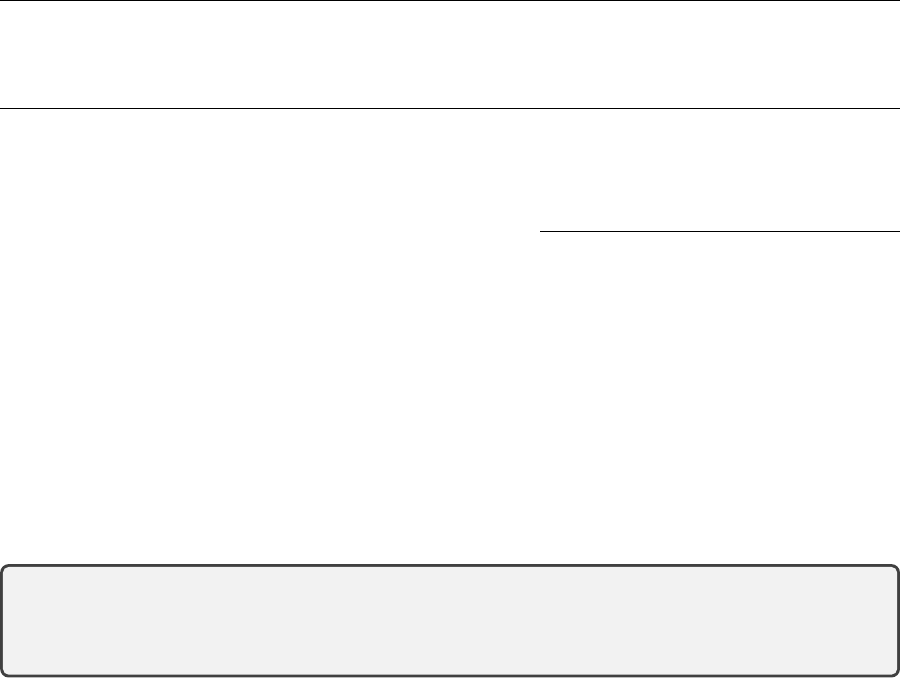
CHAPTER 5

Physical Big Data Integration

"There are two ways of spreading light: to

be the candle or the mirror that reﬂects

it."

Edith Wharton

In this chapter, we focus on our Semantic Data Integration approach, namely physical integ-

ration of heterogeneous data sources using Semantic Technologies. Semantic Data Integration

requires to convert to RDF all data coming from the input data sources, then to query the

uniform output data using SPARQL. We propose an architecture for this integration, which

we term SBDA, for Semantiﬁed Big Data Architecture. This chapter formally introduces the

proposed architecture, suggests a set of requirements that it needs to meet, and describes it in

the form of a reusable blueprint. An implementation of the blueprint is subsequently described

and evaluated comparing it to a baseline native RDF triple store. In particular, we present

our strategies for representing and partitioning the resulted to-be-queried RDF data. In this

chapter, we address the following research question:

RQ2.

Do Semantic Technologies provide ground and strategies for solving Physical

Integration in the context of Big i.e., techniques for the representation, storage and

uniform querying of large and heterogeneous data sources?

Contributions of this chapter can be summarized as follows:

•

The deﬁnition of a blueprint for a Semantiﬁed Big Data Architecture that enables the

ingestion, querying and exposure of heterogeneous data with varying levels of semantics

(hybrid data), while ensuring the preservation of semantics.

•

A proof-of-concept implementation, named SeBiDA, of the architecture using Big Data

components such as Apache Spark and Parquet.

•

Evaluation of the beneﬁts of using Big Data technology for storing and querying hybrid

large-scale data. In particular, we evaluate SeBiDA performance in ingesting and querying

increasing data sizes, while comparing it to a centralized RDF triple store.

This chapter is based on the following publication:

Chapter 5 Physical Big Data Integration

• Mohamed Nadjib Mami

, Simon Scerri, Sören Auer, Maria-Esther Vidal. Towards Seman-

tiﬁcation of Big Data Technology. International Conference on Big Data Analytics and

Knowledge Discovery (DaWaK), 376-390, 2016.

5.1 Semantiﬁed Big Data Architecture

A Semantiﬁed Big Data Architecture, SBDA [183], allows for ingesting and processing heterogen-

eous data on a large scale. In the literature, there has been a separate focus on achieving eﬃcient

ingestion and querying of large RDF data and for other structured types of data. However,

approaches for combining both RDF and non-RDF under one same architecture is overlooked.

Our Semantic Data Integration approach addresses this gap through the introduction of (1)

a uniﬁed data model and storage that is adapted and optimized for ingesting and integrating

heterogeneous data using the RDF model, and (2) uniﬁed querying over all the ingested data.

5.1.1 Motivating Example

In order to facilitate the understanding of subsequent concepts and approaches, we start by

introducing a simple motivating example. Suppose that a municipality is building a citizen-facing

online service to manage the bus network. The municipality got hold of three data sources of

various types, which they need to integrate and query in a uniform manner in order to improve

the mobility service (see Figure 5.1):

Mobility: an RDF graph containing information about Buses circulating around the city,

e.g., matriculation and size. Data is stored in NTriple ﬁles in HDFS.

Regions: JSON-encoded data containing information about the country’s Regions where

buses operate, e.g., name and surface, semantically described using ontology terms in

JSON-LD format. Data is stored in a JSON format in HDFS.

Stop: a tabular data containing information about Stops e.g., names and coordinates,

complying with GTFS speciﬁcation

. Data is stored in a Cassandra database.

The problem to be solved is providing uniaﬁed data model to store and query these datasets,

independently of their dissimilar types. Once done, the three data sources can be queried in

unity. For example, to investigate recurrent complaints about bus delays at a certain stop,

the company suspects driver unpunctuality and retrieves all bus drivers that serve that stop.

Another example, to increase bus frequency near to a recently opened university, the company

tries to relocate certain buses from other regions to the new university region. To do so, the

company retrieves the number of buses serving each region and sorts them in a descendant

order.

5.1.2 SBDA Requirements

In order to fulﬁll its objectives, SBDA should meet the following requirements:

R1: Ingest semantic and non-semantic data.

SBDA must be able to process arbitrary types

of data. We should distinguish between semantic and non-semantic data. Semantic data is all

data that is either originally represented according to the RDF data model or has an associated

https://developers.google.com/transit/gtfs/

5.1 Semantiﬁed Big Data Architecture

"@id": "regionA"

"name": "Ile-de-France",

"population": "12,005"

Stops: Cassandra table (D

)

"@context": {

"name": "plc:name",

"population": {

"@id": "plc:population",

"@type": "xsd:long"

}

Regions: JSON-LD ﬁle (D

)

stop_id stop_name stop_lat stop_long

stopA “Pyramides” 48.8666 2.3344

stopB “Concorde” 48.8656 2.3211

ex:

lat

ex:

stopBy

Mobility: RDF dataset (D

)

ex:

stop1

ex:

bus1

“1234”

“Ost”

ex:

region1

ex:

Bus

ex:

Stop

rdf:type

ex:

name

ex:

locatedIn

ex:

Region

rdf:type

ex:

driver1

ex:

driver

“5678”

ex:

long

Figure 5.1: Motivating Example. Mobility: semantic RDF graph storing information about buses;

Regions: semantically-annotated JSON-LD data about country’s regions; and (3) Stop: non-semantic

data about stops stored in a Cassandra table.

mapping, which allows to convert it to RDF. Non-semantic data is all data that is represented

in other formalisms, e.g., tabular, JSON, XML. SBDA requires to lift non-semantic data to

semantic data, which can be achieved through the integration of mapping techniques e.g.,

R2RM

, CSVW

annotation models or JSON-LD contexts

, RML [169]. This integration can

lead to either a representation of the non-semantic data in RDF or its annotation with semantic

mappings, which enable the conversion to RDF at a later stage. In our example, Mobility and

Regions are semantic data. The former is originally in RDF model, while the latter is not in

RDF model but has mappings associated that enables the conversion to RDF. Stops, on the

other hand, is a non-semantic dataset on which semantic lifting can be applied.

R2: Preserve semantics and metadata in Big Data processing chains.

Once data is prepro-

cessed, semantically enriched and ingested, it is paramount to preserve the semantic enrichment

as much as possible. RDF-based data representations and mappings have the advantage

(e.g., compared to XML) of using ﬁne-grained formalisms (e.g., RDF triples or R2RML triple

maps) that persist even when the data itself is signiﬁcantly altered or aggregated. Semantics

preservation can be reduced as follows:

•

Preserve URIs and literals. The most atomic components of RDF-based data representation

are URIs and literals

. Best practices and techniques to enable the storage and indexing

of URIs (e.g., by separately storing and indexing namespaces and local names) and literals

(along with their XSD or custom datatypes and language tags) need to be deﬁned. In

the dataset Mobility, the Literals "Alex Alion" and "12,005"xsd:long, and the URI

http://www.w3.org/TR/r2rml

http://www.w3.org/2013/csvw/wiki/Main_Page

http://www.w3.org/TR/json-ld

We disregard blank nodes, which can be avoided or replaced by IRIs [184].

Chapter 5 Physical Big Data Integration

‘http://xmlns.com/foaf/0.1/name‘ (shortened foaf:name in the ﬁgure), should be stored in

an optimal way in the big data storage. x2

•

Preserve triple structure. Atomic URI and literal components are organized in triples.

Various existing techniques can be applied to preserve RDF triple structures in SBDA

components (e.g., HBase [185–187]). In the dataset Mobility, the triple (prs:Alex

mb:drives mb:Bus1) should be preserved by adopting a storage scheme that keeps the

connection between the subject prs:Alex, the predicate mb:drives and the object mb:Bus1.

Data may not be in RDF format but annotated using semantic models by means of mapping

rules. The mappings are usually composed of ﬁne-grained rules that deﬁne how a certain

entity, attribute or value can be transformed to RDF. The preservation of such data structures

throughout processing pipelines means that resulting views or query results can also be directly

transformed to RDF. R2RML, RML, JSON-LD contexts, and CSV annotation models are

examples of mapping languages. In Regions dataset of the motivating example (Figure 5.1),

the semantic annotations deﬁned by the JSON object @context would be persisted in association

with the actual data it describes, RegionA.

R3: Scalable and Eﬃcient Query Processing.

Since the SBDA architecture targets large

data sources, Data Management techniques like data caching, partitioning, indexing, query

optimization have to be exploited to ensure the scalable and eﬃcient performance of query

processing. For example, cache in memory the triples that have the most frequently accessed

predicates, partition on disk the data in a certain scheme that minimizes data transfer across

compute nodes, index the data for fast retrieval of RDF objects when subject and predicate are

known, query rewriting to reduce joins, etc.

5.1.3 SBDA Blueprint

We represent the SBDA architecture as a generic blueprint that can be instantiated using

various processing and query technologies. The only ﬁxed decision we made is the choice of

the target data model, which we suggest to be tabular following the prevalence of this model

in Big Data technologies. Historically, the relational data model and RDBMSs backed several

state-of-the-art RDF centralized triple stores [188–190]. The tendency persists with the modern

RDF distributed storage and processing systems, which we will review in the Related Work

of this thesis (Chapter 3). In this section, we provide a formalisation of the various concepts

underlying the SBDA blueprint.

Deﬁnition 1 (Heterogeneous Input Superset)

We deﬁne a heterogeneous input superset HIS, as

the union of the following three types of datasets:

• D

, . . . , d

is a set of non-semantic, structured or semi-structured, datasets in

any format (e.g., relational database, CSV ﬁles, Excel sheets, JSON ﬁles).

• D

. . . , d

is a set of semantically annotated datasets, consisting of pairs of

non-semantic datasets with corresponding semantic mappings (e.g., JSON-LD context,

metadata accompanying CSV).

• D

, . . . , d

is a set of semantic datasets consisting of RDF triples.

5.1 Semantiﬁed Big Data Architecture

In our motivating example, stops, regions, and mobility correspond to

, and

respectively.

Deﬁnition 2 (Dataset Schemata)

Given HIS=

∪ D

, the dataset schemata of

and D

are deﬁned as follows:

• S

, . . . , s

}

is a set of

non-semantic schemata structuring D

, where each

deﬁned as follows:

= {(T, A

) | T is an entity type and A

is the set of all the attributes of T}

• S

, . . . , s

}

is a set of the

semantic schemata behind D

where each

is deﬁned

as follows:

= {(C, P

) | C is an RDF class and P

is the set of all the properties of C

}

• S

, . . . , s

}

is a set of the

semantic schemata annotating D

where each

deﬁned the same way as elements of S

In the motivating example, the semantic schema of the dataset

mobility is:

= {(ex:Bus, {ex:matric, ex:stopsBy}), (ex:Driver, {ex:name, ex:drives})}

Deﬁnition 3 (Semantic Mapping)

A semantic mapping is a relation linking two semantically-

equivalent schema elements. There are two types of semantic mappings:

• m

= (e, c) is a relation mapping an entity type e from S

onto a class c.

• m

= (a, p) is a relation mapping an attribute a from S

onto a predicate p.

SBDA facilitates the lifting of non-semantic data to semantically annotated data by map-

ping non-semantic schemata to RDF vocabularies. The following are possible mappings:

(stop_name, rdfs:label), (stop_lat, geo:lat), (stop_long, geo:long).

Deﬁnition 4 (Semantic Lifting Function)

Given a set of mappings

and a non-semantic data-

set

, a semantic lifting function

returns a semantically-annotated dataset

with semantic

annotations of entities and attributes in d

In the motivating example, dataset Stops can be semantically lifted using the following

set of mappings: {(stop_name, rdfs:label),(stop_lat, geo:lat), (stop_long, geo:long)}, thus a

semantically annotated dataset is generated.

Deﬁnition 5 (Ingestion Function)

Given an element

d ∈ HIS

, an ingestion function

(

)

returns a set of triples of the form (R

, A

, f ), where:

• T an entity type or class for data on d,

• A

is a set of attributes A

, . . . , A

of T ,

A set of properties P

of an RDF class C where: ∀ p ∈ P

(p rdfs:domain C).

Here again, for simplicity, we use the exemplary namespace preﬁx ex, which can denote any given ontology.

Multiple ontology namespace preﬁxes can also be used e.g., ex1, ex2.

Chapter 5 Physical Big Data Integration

• R

⊆ type

(

)

× type

(

)

× · · · × type

(

)

⊆ d

, where

type

(

) =

indicates that

the data type of the attribute A

in d, and

• f

× A

→

∈A

type

(

) such that

(

t, A

) =

indicates that

∈ tuple t

is the value of the attribute A

The result of applying the ingestion function

over all

d ∈ HIS

is the ﬁnal dataset that we

refer to as Final Dataset F D.

F D =

∈HIS

In(d

)}

Deﬁnition 6 (Data Queries)

Let

be a relational query on relations

F D

. We deﬁne a

Querying function R that generates a view v over the transformed dataset

F D

given a query

R(F D, q) = r

n×w

= v

• r

is a matrix containing

rows, which represent the results, and w columns, which

correspond to the query variables.

• r

prov

is a metadata matrix containing provenance information (source dataset(s) links,

acquisition timestamp) for each element of the resulting matrix.

• q is retained as the query generating v.

The set of all views is denoted by V .

These concepts are visually illustrated in Figure 5.2. The SBDA blueprint handles a repres-

entation (

F D

) of the relations resulting from the ingestion of multiple heterogeneous datasets in

HIS

(

, d

). The ingestion (In) generates relations or tables (denoted

) corresponding

to the data, supported by a schema for interpretation (denoted

and

). The ingestion of

semantic (

) and semantically-annotated (

) data is direct (denoted respectively by the solid

and dashed lines), a non-semantic dataset (

) can be semantically lifted (SL) given an input

set of mappings (M). Query processing can then generate a number (

|Q|

) of results over (

F D

5.2 SeBiDA: A Proof-of-Concept Implementation

We validate our blueprint through the description of a proof of concept implementation, called Se-

BiDA (for

mantiﬁed

ata

rchitecture). It comprises the following three main components

(Figure 5.3), which are subsequently detailed:

•

Schema Extractor: It performs schema knowledge extraction from an input data source

and performs semantic lifting based on a provided set of mappings.

•

Data Loader: It creates tables based on the extracted schemata and loads input data

accordingly.

• Data Server: It receives queries and generates results as tuples or RDF triples.

The ﬁrst two components jointly realize the ingestion function

from subsection 5.1.3. The

resulting tables FD can then be queried using the Data Server to generate the required views.

5.2 SeBiDA: A Proof-of-Concept Implementation

Figure 5.2: A Semantiﬁed Big Data Architecture Blueprint.

5.2.1 Schema Extractor

We extract the structure of both semantic and non-semantic data to transform it into the tabular

model, an operation that is commonly called ﬂattening. The schema extraction mechanism

varies from a data source to the other:

(A)

From the semantic or semantically-annotated input datasets (

), we extract classes

and properties describing the data (see Deﬁnition 2). In the presence of RDF schema,

classes and properties can be extracted by querying it. If not, schema information is

extracted by exhaustively parsing the data. For example, this can be achieved by ﬁrst

reformatting RDF data into the following representation:

(class, (subject, (predicate, object)

)

which reads: "Each class has one or more instances where each instance can be described

using one or more (predicate, object) pairs", and then we retain the classes and properties.

The XSD datatypes, if present, are leveraged to type the properties, otherwise

string is

used.

(B)

From each non-semantic input dataset (

), we extract entities and attributes (cf. Deﬁni-

tion 2). For example, in relational and some NoSQL databases, entities and attributes

correspond respectively to tables and columns, which can be retrieved by querying a set of

default metadata tables. Another example, the entity and its attributes can be extracted

from a CSV ﬁle’s name and header, respectively. Whenever possible, attribute data types

When the object is occasionally not typed or is a URL.

Chapter 5 Physical Big Data Integration

Figure 5.3: SeBiDA General Architecture. Data and work ﬂows start from the left to the right. Insets

are input sets: (a) semantic and semantically-annotated data schema, (b) non-semantic data schemata,

are extracted, otherwise, string is used. Schemata that do not natively have a tabular

format (e.g., XML, JSON) also undergo ﬂattening into entity-attributes pairs. Although

principally diﬀerent from the relational/tabular model, it is common to ﬁnd non-tabular

data organized into repeated schema-ﬁxed tuples that can be extracted and saved into

tables. For example, modern processing engines e.g., Apache Spark, do not accept the

conventional single-rooted JSON ﬁles, but a variation called JSON Lines

where each line

is a separate valid JSON value. This enables these engines to load JSON ﬁles and query

them using their regular schema. The same is observed for XML ﬁles, which may contain

a ﬂat ordering of elements from which a regular schema can be extracted. One may not

reinvent the wheel and use oﬀ-the-shelf some of the modern specialized processing engines

that support the extraction of data from various sources. We use in our implementation

Apache Spark

(see Figure 5.3) and it has wrappers

for many popular data sources,

which can be used to extract schema information from JSON, XML, NoSQL databases,

etc.

As depicted in Figure 5.3, schema extraction is performed independently and prior to data

loading. Extracted schema information is saved in an independent metadata store. This is

important because it allows the user to visualize the schema, navigate through it, and formulate

queries accordingly. In our SeBiDA implementation, we use MongoDB

, which is a ﬂexible

schema-less document-based store.

http://jsonlines.org

https://spark.apache.org

https://spark-packages.org

https://www.mongodb.org

5.2 SeBiDA: A Proof-of-Concept Implementation

Source Target Datatype

stop_name http://xmlns.com/foaf/0.1/name String

stop_lat http://www.w3.org/2003/01/geo/wgs84_pos#lat Double

stop_lon http://www.w3.org/2003/01/geo/wgs84_pos#long Double

parent_station http://example.com/sebida/parent_station String

Table 5.1: Mapping data attributes to ontology properties with datatype speciﬁcation.

5.2.2 Semantic Lifter

In this step, SeBiDA targets the lifting of non-semantic entities/attributes to existing ontology

classes/properties. The lifting process is semi-automated. We auto-suggest ontology terms

based on the syntactical similarity with the entities/attributes. If semantic counterparts are

undeﬁned, internal URIs are created by attaching a base URI. Otherwise, the user can adjust

the suggestions or incorporate custom ones. Table 5.1 shows a result of this process, where

four attributes from the entity ’Stop’

have been mapped to existing vocabularies, where the

forth converted to an internal URI. In our implementation, semantic mappings are stored in

the same MongoDB metadata store in the form of simple one-to-one relationships, and thus

can be visually explored. However, RDF-based mapping standards (e.g., R2RML [

das2011r2

RML [169]) can also be used. The latter are even more favorable if more sophisticated mapping

speciﬁcation is required. Being in RDF, these standards also enable the interoperability across

systems or implementations.

5.2.3 Data Loader

This component loads data from the source HIS into the ﬁnal dataset FD. First, it generates

tables following a tailored partitioning scheme. Then, it loads data into the tables accordingly.

Table Generation

Tables are generated following the previously extracted schema (subsection 5.2.1). For each

class, a corresponding table template is created as follows:

(A)

For Semantic Data, a table with the same label is created for each

class

(e.g. a table

`ex:Bus`

from the RDF class ex:Bus). A default column ’ID’ (of type string) is created

to store the triple’s subject. For each

predicate

describing the class, an additional column

is created typed according to the

predicate

extracted data type. This representation

corresponds to the Property Table scheme [55], and more speciﬁcally its class-based

clustering variant. In the latter, triples are distributed into tables based on their RDF

type [189]. This Property Table partitioning scheme is used by traditional centralized triple

stores e.g, Sesame, Jena2, RDFSuite and 4store [189]. A particularity in our approach is

the ability to capture the classes of multi-typed RDF instances. For every table template,

an extra column of array type called "alsoType" is added, which is intended to store every

extra type found attached to one same RDF instance. Further, a boolean column called

type ﬂag column is added to the table template whenever an instance of an otherType is

detected. In the previous example, two type ﬂag columns are added also_Electric and

also_Mini-bus. Observe the schema of the table in Figure 5.4.

developers.google.com/transit/gtfs/reference

Chapter 5 Physical Big Data Integration

(B)

For non-Semantic data, for each

entity

, a table is similarly created as above, taking the

entity label as table name and creating a typed column for each attribute. We assume that

multi-typing is only a prevalent property in semantic data, and thus we do not consider

the problem of scattering data across several tables.

For RDF data, since not all instances have values to all the predicate, the tables may end

up storing lots of null values, and thus reserving unnecessary storage space. However, this

concern has largely been reduced following the emergence of modern NoSQL databases (e.g.,

HBase), and columnar storage formats (e.g., Apache Parquet), where the null values do not

occupy a physical space. The particularity of columnar formats is that tuples are physically

stored column-by-column instead of line-by-line. With this organization, all values of the same

column are of the same type, in contrast to values of the same row that are of diﬀerent types.

This value homogeneity enables eﬃcient compression e.g., by skipping the unnecessary

null

values (run-length encoding [191]). Another advantage of the columnar data layout is schema

projection, whereby only projected columns are read and returned following a query. Using the

columnar format for solving this so-called table sparsity problem is witnessed in the literature

of centralized RDF stores, e.g., in [191]

In our implementation, we use Apache Spark to perform the data loading. We leverage its

numerous wrappers to ingest as many data sources as possible. We only resort to building our

custom reader when no wrapper is available, which is the case of RDF data. For storing the

loaded data, we use the column-oriented tabular format Apache Parquet

, which allows to

overcome the sparsity problem. Parquet is suitable for storing RDF data from other respects.

It also supports composed and nested columns, i.e., saving multiple values in one column and

storing hierarchical data in one table cell. This is a common occurrence in RDF where one

instance may use the same predicate several times, e.g.,

_:authoredBy

predicate. Parquet

also involves state-of-the-art encoding methods, e.g., bit-packing, run-length, and dictionary

encoding. In particular, the latter can be useful to store long strings, which is the case of URIs.

Finally, Parquet ﬁles are saved inside Hadoop Distributed Filesystem (HDFS), which is the de

facto distributed ﬁle system for Big Data applications. This makes it so that other processing

engines can inter-operate and query the same data generated by SeBiDA. This is not a design

choice of ours, but rather a common understanding across modern Big Data applications leading

to the emergence of so-called Hadoop Ecosystem [192]. In the latter, Hadoop Distributed File

System is used as the central data repository from which the various processing frameworks

read raw data.

Table Population

Once the table template is created, the table is populated as follows:

For each RDF extracted class (see subsection 5.2.1) iterate through its instances, a new

row is inserted for each instance into the corresponding table. The instance subject is

stored in the ’ID’ column, whereas the corresponding objects are saved under the column

representing the predicates. Multi-typed instances are stored following the design style

described above (Table Generation). See Figure 5.4 for a visual illustration. If an instance

is of Bus, Electric and Mini-bus types, it is stored in the Bus table, the other types

are added to the alsoType array column, and

true

is set as the value to the type ﬂags

also_Electric and also_Mini-bus.

https://parquet.apache.org

5.2 SeBiDA: A Proof-of-Concept Implementation

ex:bus1

rdf:type

ex:Bus ; ex:Electric ; ex:Mini-bus .

ex:bus1 ex:name "600"^^xsd:integer .

ex:bus1 ex:driver ex:driver1 .

ex:bus2

rdf:type

ex:bus ; ex:Electric .

ex:bus2 ex:name "601"^^xsd:integer .

ex:bus2 ex:driver ex:driver2 .

string

ex:name

int

ex:driver

string

aslo_Electric

boolean

also_Mini-bus

boolean

alsoType

Array[String]

ex:bus1 "600"

ex:driver2 true true

[“ex:Electric”,”ex:Mini-bus”]

ex:bus2 "601"

ex:driver2 true false

[“ex:Electric”]

Table ex:Bus

load

Figure 5.4: Storing two RDF instances into

ex:Bus

table while capturing their multiple types. Data

types are also captured, e.g., xsd:integer (XML Integer type) to table integer type.

In the presence of multiple types, we sort the types lexicographically and use the latest

for the to-be-populated table. This way, instances of similar types end up in the same

table, thus, we reduce data scattering. However, other types can be selected, e.g., the

most used type or, in the presence of schema, the most speciﬁc or generic, etc. The most

and generic types can be extracted from the class hierarchy, provided that an adequate

RDF schema is available. The most and least used types can be obtained by computing

statistics e.g., during the loading process. Each choice has its impact on data distribution

and, thus, query performance. For example, using the most generic type from the class

hierarchy (e.g., Bus) would result in a skewed large table containing potentially too many

instances; however, the table would store all the data of that type and no union is required.

If, however, a less generic class is used (e.g., Mini-bus) to build the table, and if a query

asks for instances from the top-level generic class (e.g., Bus), a union with all the less

generic tables is required.

Table population in the case of non-semantic data varies according to the data type. For

example, we iterate through each CSV line and save its values into the corresponding

column of the corresponding table. XPath and JSONPath [193] can be used to iteratively

select the needed nodes in XML and JSON ﬁles, respectively. Technically, thanks to their

versatility, many modern technologies allow to extract, transform and load (ETL) data.

This makes the overall integration process simpler and more cost-eﬀective since data is read

and written without requiring intermediate data materialization. In our implementation,

Apache Spark enables us to read data from the heterogeneous sources and load it under

our uniﬁed partitioning and storage layout.

5.2.4 Data Server

Data loaded into tables following the uniﬁed tabular layout can be accessed in an ad hoc manner

by means of queries. The Data Server is the component responsible for receiving and performing

query processing and representing the ﬁnal results.

Chapter 5 Physical Big Data Integration

SELECT ?n ?d {

?b ex:driver ?d .

?b ex:name ?n .

FILTER (?n != "500")

}

SELECT ex:name, ex:driver FROM ex:Bus

UNION

SELECT ex:name, ex:driver FROM ex:Mini-bus

UNION

SELECT ex:name, ex:driver FROM ex:Electric

WHERE ex:name != "500"

Figure 5.5: From SPARQL to SQL with SQL Query Expansion to involve instances of the same type

scattered across multiple tables.

Querying Interface

Since our SBDA architecture and implementation propose a tabular-based model for representing

the integrated data, the data itself is accessed using SQL query language. However, semantic

data is more naturally accessed using SPARQL. Therefore, a custom SPARQL-to-SQL conversion

method should be designed to access the data. SPARQL-to-SQL methods exist in the literature,

but they cannot be adopted as-is to our custom data partitioning scheme, i.e., Class-based

Multi-Type-Aware Property Tables. We generally follow a simple direct translation, similarly

to [62], beneﬁting from the analogous semantics of several basic SQL and SPARQL (e.g.,

SELECT

FILTER

ORDER BY

GROUP BY

LIMIT

). We diﬀer from [62], however, in that we apply

UNION

whenever instances of the same type are scattered across multiple tables. To reconcile this

scattered data, we use the Query Expansion algorithm described in Listing 5.1 and illustrated

in Figure 5.5. We call the table addressed in the SQL query (after

FROM

) the Main Table,

e.g.,

ex:Bus

in Figure 5.5. The algorithm aims at performing a query rewriting to include the

other tables where instances of the same type as the Main Table can be found. To decide on

whether a union is needed and what are the complementary tables to union, the Data Server

visits the schema and looks for any table that has the Main Table name as a ﬂag column, i.e.,

also_{MainTable}, (Lines 7 and 8). This is one rationale behind keeping the schema separately

stored as metadata. If a table is found, a

SELECT

query is added as a

UNION

with the

SELECT

of the input SQL query. If other tables are found, they are similarly added as

UNION

to the

previous query, etc. (Lines 9 and 10). In SQL standard, there are two requirements for the

UNION operator that have to be met:

The involved

SELECT

statements should include columns of analogous types. This condition

is met as the user conceptually searches for the columns of the same entity, they are just

physically found in disperse tables. The types are preserved by the Data Loader, which is

the component responsible for populating the various tables containing instances of the

same type.

2. The involved SELECT statements should have the same number of columns. This require-

ment is also met as the rewriting operation is done automatically by the Data Server

without manual user intervention.

5.3 Experimental Study

?n ?d

"600"

ex:driver1

"601"

ex:driver2

SELECT ?n ?d {

?b ex:driver ?d .

?b ex:name ?n .

FILTER (?n != "500")

}

ex:res1 ex:name "600"

ex:res1 ex:driver ex:driver1

ex:res2 ex:name "601"

ex:res2 ex:driver ex:driver2

Query

Results: table Results: triples

Figure 5.6: A SPARQL query (left) returning results represented in tables (middle) or triples (right).

1 Input : query , FD

2 Output : n ewQuery

4 mainT ab le = table ( query )

5 new Query = que ry // i.e . , " SE LEC T ... FROM { m ai nT able } ..."

7 foreach table in FD

8 if s chema_c ol umns ( table ) co ntains also_ { mainTable }

9 newQu er y = newQue ry + " UNION SELECT { co lumns } from { table } " +

10 " WHERE als oO fT ype_ { table }= true "

Listing 5.1: Query Expansion rewriting to include all tables containing all instances of the same type.

Multi-Format Results

The Data Server can return the query results both as a table or as an RDF graph. The table is

the default results representation stemming both from the underlying tabular data model and

from the query engine used, Apache Spark. The process of RDFisation is achieved as follows:

Create a triple from each projected column, using the column name and value as the triple

predicate and object, respectively. For the triple subject, if the results include one table ID

column, use its value as the triple subject. Otherwise, set the subject to <base-URI /res_

{

}

where the base URI is deﬁned by the user, and i is an auto-incrementing integer. See Figure 5.6

for an example of a query and its two result formats, where ex is the preﬁx of an exemplary

base URI https://example.com/data.

5.3 Experimental Study

The goal of this experimental study is to evaluate to what extent SeBiDA

meets the require-

ments

, and

(see subsection 5.1.1). Namely, ingest both semantic and none-semantic

data, preserve data semantics after the ingestion and during query processing, and exploiting

the eﬀect of BDM techniques, in particular caching, on query execution time.

5.3.1 Experimental Setup

Datasets

We use the Berlin Benchmark [194] to generate both semantic and non-semantic data. We use

the formats N-Triple and XML, for semantic and non-semantic data respectively, both produced

https://github.com/EIS-Bonn/SeBiDA

Chapter 5 Physical Big Data Integration

RDF Dataset Size Type Scale Factor (# products)

Dataset

48.9GB RDF 569,600 (200M)

Dataset

98.0GB RDF 1,139,200 (400M)

Dataset

8.0GB XML 284,800 (100M)

Table 5.2: Description of the Berlin Benchmark RDF Datasets. The original RDF data is in plain-text

N-Triple serialization format.

RDF Dataset Loading Time New Size Ratio

Dataset

3960 sec 389MB 1:0.008

Dataset

10440 sec 524MB 1:0.005

Dataset

1800 sec 188MB 1:0.023

Table 5.3: Data Loading performance. Shown are the loading times, the sizes of the obtained data, and

the ratio between the new and the original sizes.

using BSBM data generator

. Table 5.2 describes the generated data in terms of the number of

triples and ﬁle size.

Queries

We evaluate with all 12 BSBM SQL queries, which are slightly adapted to match the SQL

supported syntax of the underlying query engine, Apache Spark. We use

LEFT OUTER JOIN

and inner queries instead of

OPTIONAL

and

NOT IN

sub-queries; the latter being unsupported

We also omit time ﬁlter and RDF object language comparison, which are also not supported.

Filtering based on the language tag is a speciﬁc function to the RDF data model, so not present

at the SQL query.

Metrics

We measure the loading time of the datasets, the size of the datasets after the loading, as well

as the query execution time over the loaded datasets. The queries are run both against a cold

cache and a warm cache. Running on cold cache eliminates the impact of any possible previously

computed intermediate results. Warm cache is running the ﬁve queries after having run the

query once before, which reuses some temporary internal data during the subsequent runs of

the same query. The query execution is run 10 times and the average time is reported, with a

timeout of 300 seconds (5 minutes). Loading timeout is 43200 seconds (12 hours).

Environment

All queries are run on a cluster of three nodes having DELL PowerEdge R815, 2x AMD Opteron

6376 (16 cores) CPU and 256GB RAM, and 3 TB SATA RAID-5 disk. Queries are run in a cold

cache and warm cache. To run on cold cache, we clear the cache before running each query

Using a command line:

./generate -fc -pc [scaling factor] -s [file format] -fn [file name]

, where

ﬁle format is nt for semantic data and xml for non-semantic XML data.

At the time of conducting these evaluations.

Using a dedicated Linux system command: sync; echo 3 > /proc/sys/vm/drop_caches

5.3 Experimental Study

Dataset

Q1 Q2 Q3 Q4 Q5 Q6 Q7 Q8 Q9 Q10 Q11 Q12 Geom. Mean

Cold

Cache 3.00 2.20 1.00 4.00 3.00 0.78 11.3 6.00 16.00 7.00 11.07 11.00 4.45

Warm

Cache 1.00 1.10 1.00 2.00 3.00 0.58 6.10 5.00 14.00 6.00 10.04 9.30 3.14

Diﬀ. 2.00 1.10 0 2.00 0 0.20 5.20 1.00 2.00 1.00 1.03 1.70 1.31

Ratio 3.00 2.00 1.00 2.00 1.00 1.34 1.85 1.20 1.14 1.17 1.10 1.18 1.42

Dataset

∪ Dataset

Q1 Q2 Q3 Q4 Q5 Q6 Q7 Q8 Q9 Q10 Q11 Q12 Geom. Mean

Cold

Cache 3.00 2.94 2.00 5.00 3.00 0.90 11.10 7.00 25.20 8.00 11.00 11.5 5.28

Warm

Cache 2.00 1.10 1.00 5.00 3.00 1.78 8.10 6.00 20.94 7.00 11.00 9.10 4.03

Diﬀ. 1.00 1.84 1.00 0 0 -0.88 3.00 1.00 4.26 1.00 0 2.40 1.22

Ratio 1.50 2.67 2.00 1.00 1.00 0.51 1.37 1.17 1.20 1.14 1.00 1.26 3.70

Table 5.4: Benchmark Query Execution Times (seconds). in Cold and Warm Caches. Signiﬁcant

diﬀerences are highlighted in bold.

5.3.2 Results and Discussions

For data loading time, the results in Table 5.3 show that semantic data loading takes between 1

to 3 hours, whereas non-semantic XML data loading time takes 0.5 hours. In the absence of a

schema, the loading of semantic data requires to exhaustively parse all the data and reorganize

it to correspond with our tabular model (ﬂattening). During this process, an inevitable large

data movement occurs (Spark

collect

function), causing a signiﬁcant network transfer and,

thus, negatively impacting query performance. A small technique that we employed and that

improved the loading time was reversing the URIs of RDF objects. It allowed for faster sorting

and more balanced data distribution. The tables extracted from the semantic data are product,

oﬀer, vendor, review, person and

producer

, which correspond exactly to the main tables of

the BSBM relational representation. Similar tables are retrieved from XML data, which are

accessed using Spark XML reader

by means of XPath calls. However, we achieve a substantial

gain in terms of data size due to the adopted data model that avoids data repetition (in case of

RDF data) and the used ﬁle format (Parquet) that performs very eﬃcient data compression

(see subsection 5.2.3).

Table 5.4 reports on the results of executing Berlin Benchmark 12 queries against

Dataset

(ori-

ginally semantic), alone and in combination with

Dataset

(originally non-semantic). Table 5.5

reports on the same but using

Dataset

(originally semantic) instead of

Dataset

. Queries are

run on cold cache and then on warm cache. The results show that all queries ﬁnished far below

the speciﬁed threshold (300s), with the fastest query being Q6 ﬁnishing in 0.78s cold and 0.58s

warm, and the slowest query being Q9 ﬁnished in 25.2s cold and 20.94s warm. Among the 12

For more details: https://github.com/databricks/spark-xml

Chapter 5 Physical Big Data Integration

Dataset

Q1 Q2 Q3 Q4 Q5 Q6 Q7 Q8 Q9 Q10 Q11 Q12 Geom. Mean

Cold

Cache 5.00 3.20 3.00 8.00 3.00 1.10 20.00 7.00 18.00 7.00 13.00 11.40 6.21

Warm

Cache 4.00 3.10 2.00 7.00 3.00 1.10 18.10 6.00 17.00 6.00 12.04 11.2 5.55

Diﬀ. 1 0.1 1 1 0 0 1.9 1 1 1 0.96 0.2 0.66

Ratio 1.25 1.03 1.50 1.14 1.00 1.00 1.10 1.17 1.06 1.17 1.08 1.02 1.12

Dataset

∪ Dataset

Q1 Q2 Q3 Q4 Q5 Q6 Q7 Q8 Q9 Q10 Q11 Q12 Geom. Mean

Cold

Cache 11.00 3.20 7.20 17.00 3.00 1.10 23.10 16.00 20.72 10.00 14.10 13.20 8.75

Warm

Cache 4.00 3.20 2.00 8.00 3.00 1.10 21.20 8.00 18.59 7.00 12.10 11.10 5.96

Diﬀ. 7 0 5.2 9 0 0 1.9 8 2.13 3 2 2.1 2.79

Ratio 2.75 1.00 3.60 2.13 1.00 1.00 1.09 2.00 1.11 1.43 1.17 1.19 1.47

Table 5.5: Benchmark Query Execution Times (seconds). in Cold and Warm Caches-Signiﬁcant diﬀerences

are highlighted in bold

queries, the most expensive queries are Q7 to Q12. Q7 is the most complex joining the largest

number of tables (four), followed by Q9 and Q12 joining three tables producing a large number

of intermediate results (in the absence of ﬁlters). Q8 and Q10 are similar in that they join two

tables while sorting the ﬁnal results. Q11 accesses the largest table (oﬀer) ﬁltering on a string

value that does not exist in the data. Q1 to Q6 belong to the lower end of query execution time.

Q1 query accesses only one table and has two selective ﬁlters. Q2 joins two tables, but one

table is small in addition to ﬁltering the results to a speciﬁc operand ID. Q3 and Q5 contain

a self-join (one table), but largely limit the intermediate results by incorporating ﬁve and six

ﬁlters, respectively. Q4 contains a union but accesses only one table with two ﬁlters. Q6 is the

simplest and smallest query with only one ﬁlter. Note that for this query, the diﬀerence between

the warm and cold cache execution is negative. This means that the query execution on the

cold cache was faster than that on the warm cache. This is plausible with fast queries ﬁnishing

within a second or two as there might be a variable overhead either from the system or the

query engine that dominates the query execution time.

Further, the results in Table 5.4 and Table 5.5 suggest that caching can signiﬁcantly improve

query performance by up to 3 times saving up to 9 seconds (signiﬁcant diﬀerences highlighted in

bold). Thus, we obtain evidence of the beneﬁts of using the cache stored during previous runs

by the query engine, Spark. Finally, results also show that including data from (originally XML)

Dataset

using

UNION

operator in the 12 queries does not deteriorate query performance. This

is because the data eﬀectively queried is in Parquet format generated during XML ingestion,

which is the same format as

Dataset

and

Dataset

. This is evidence that hybrid semantic and

non-semantic data can be uniformly integrated and queried using a single query (

). Further,

we were able to capture the semantics of the data in our suggested RDF data partitioning

5.4 Summary

RDF Dataset Loading Time New Size Ratio to Parquet S ize

Dataset

93min 21GB 55:1

Dataset

Timed out - -

Table 5.6: Loading Time of RDF-3X.

Engine Q1 Q2 Q3 Q4 Q5 Q6 Q7 Q8 Q9 Q10 Q11 Q12

SeBiDA 3.00 2.20 1.00 4.00 3.00 0.78 11.3 6.00 16.00 7.00 11.07 11.00

RDF-3X 0.01 1.10 29.213 0.145 1175.98 2.68 77.80 610.81 0.23 0.419 0.13 1.58

Table 5.7: SeBiDA vs. RDF-3X Query Execution Times (seconds). Cold Cache only on

Dataset

Signiﬁcant diﬀerences are highlighted in bold.

scheme (

). Finally, the exploitation of caching and columnar-oriented format allowed us to

optimize query performance (Q3).

5.3.3 Centralized vs. Distributed Triple Stores

We can regard SeBiDA as a distributed triple store as it can load and query semantic RDF

data. Therefore, in the next series of evaluation, we compare SeBiDA’s performance against

the performance of a popular RDF store, RDF-3X [195]

. We evaluate both the loading and

querying of semantic data, the results of which are respectively shown in Table 5.6 and Table 5.7.

Loading timeout is 43200 seconds (12 hours).

Loading time shows that RDF-3X loaded

Dataset

within 93 minutes, compared to 66 minutes

in SeBiDA. Loading

Dataset

, RDF-3X exceeded the timeout threshold and took up to 24

hours before we manually terminate it. The witnessed low loading performance in RDF-3X

is attributed to the exhaustive creation of six triple indexes. These indexes also take a much

larger disk footprint in comparison to SeBiDA with a factor of 55. SeBiDA, on the other

hand, generates a much-reduced data thanks to its partitioning scheme and highly-compressed

generated Parquet tables.

For query execution time, Table 5.7 reveals no deﬁnitive winner, but show that SeBiDA in

all queries does not exceed the cap of 20s, while RDF-3X does in four queries (Q3, Q5, Q7,

Q8) and even passes to the order of minutes. We do not report on the query time of

Dataset

using RDF-3X as data was not loaded. This comparison practically supports the proposition

we made in Chapter 2 that modern highly eﬃcient and scalable formats, such as Parquet, can

compensate for the lack of indexes in improving query execution by using optimized internal

data structures and data encoding (R3).

5.4 Summary

The experimental series allows us to draw the following conclusions. The loading phase can be a

bottleneck in the overall Data Integration process. Noticing the loading time of the Semantic

data

Dataset

and

Dataset

, there seems to be a proportionality between the data size and

loading time. Namely, loading

Dataset

took double the time taken by

Dataset

; similarly, the

scale size of

Dataset

is double that of

Dataset

. Loading larger datasets, e.g., billion triples,

https://github.com/gh-rdf3x/gh-rdf3x

Chapter 5 Physical Big Data Integration

would clearly jeopardize the Data Integration process. For non-semantic data, loading the small

XML

Dataset

was also comparatively long. Although it has 16% of

Dataset

size, it took

50% of its loading time. This adds to the price of reintegrating the data when the sources

have received more data after the ﬁrst integration. These costs include schema evolution and

alignment in case the data has changed at the level of schema, data de-duplication to avoid

inserting previously inserted data, synchronization in case the data itself has been altered, etc.

A complex data loading phase hinders the adoption of the Physical Integration in many use

cases, e.g., where data dynamicity and freshness are strong requirements.

Although our Class-based Multi-Type-Aware Property Table partitioning and clustering

scheme optimizes for the loaded data footprint and query execution time, it cannot answer

queries when the predicate is unbound. However, it has been shown in the literature that such

queries are rare [54]; the same choice was made by other similar eﬀorts as reported in the Related

Work (chapter 3).

The data loading bottleneck provides the rationale behind the second part of this thesis,

namely the Virtual Integration of heterogeneous and large data sources. A virtual integration

implies that queries are posed against the original data on demand, without requiring any prior

data transformation and loading. We hypothesize that a Virtual Integration will alleviate the

ingestion overhead, but will shift the overhead to the query processing phase. This is because

the underlying data is dissimilar in nature and disparate across multiple sources, in contrast to

a fully homogeneous and centralized environment in the Physical Integration.

CHAPTER 6

Virtual Big Data Integration - Semantic Data

Lake

"Do not go where the path may lead, go

instead where there is no path and leave a

trail."

Ralph Waldo Emerson

As previously mentioned (Introduction Chapter 1), multiple and diverse data models and

distributed Data Management systems have emerged in recent years to alleviate the limitation

of traditional centralized Data Management. A prominent example is the NoSQL non-relational

family which includes models like Key-value, Document, Columnar, and Graph. Consequently,

organizations are purposely converging towards these new models in order to capitalize on their

individual merits. However, this paradigm shift poses challenges on the way of achieving a pure

Physical Data Integration, such as:

•

It is cumbersome to impossible migrating all the collected heterogeneous data to a single

universal model without incurring data loss, both in structure and semantics. For example,

nested and multi-valued array data in a document format cannot be converted in a ﬂat tabu-

lar format. Similarly, graph data cannot be straightforwardly transformed into a document

format without incorporating variable levels of normalization and denormalization.

•

Data transformation and migration incurs a signiﬁcant cost, both in time and resources.

Migrating very large data volumes requires investing in more storage and network resources,

adding to the already resource-consuming original large data.

•

Many organizations are less likely to sacriﬁce data freshness especially with the advent of

streaming and IoT technologies. Another data source added to the pool adds a complexity

level to the overall Data Integration processes.

Further, we have witnessed some of the issues that arise from exhaustively transforming

data following a purely Physical Data Integration process (reported in section 5.4). In the

Logical Data Integration, heterogeneous data sources are accessed directly in their raw format

without requiring prior data transformation and enforcing centralization. Keeping data in its

raw format not only promises freshness but also makes data available to any type of processing

Chapter 6 Virtual Big Data Integration - Semantic Data Lake

e.g., analytics, ad hoc querying, search, etc. The repository of heterogeneous data sources in

their original formats is commonly referred to as Data Lake [196]. In this chapter, we describe

our approach that leverages Semantic Web techniques to enable the ad hoc querying of Data

Lakes, called Semantic Data Lake. In particular, we address the following research question:

RQ3.

Can Semantic Technologies be used to incorporate an intermediate middleware

that allows to uniformly access original large and heterogeneous data sources on demand?

Contributions of this chapter can be summarized as follows:

•

We provide a thorough description of the concepts and components underlying the Semantic

Data Lake.

•

We suggest six requirements that need to be fulﬁlled by a system implementing the

Semantic Data Lake.

• We detail the distributed query execution aspects of the Semantic Data Lake.

This chapter is based on the following publications:

• Mohamed Nadjib Mami

, Damien Graux, Simon Scerri, Hajira Jabeen, Sören Auer, Jens

Lehmann. Uniform Access to Multiform Data Lakes Using Semantic Technologies. In

Proceeding of the 21st International Conference on Information Integration and Web-based

Applications & Services Proceedings (iiWAS), 2019.

• Mohamed Nadjib Mami

, Damien Graux, Simon Scerri, Hajira Jabeen, Sören Auer, Jens

Lehmann. Squerall: Virtual Ontology-Based Access to Heterogeneous and Large Data

Sources. In Proceeding of the 18th International Semantic Web Conference (ISWC)

229-245, 2019.

• Mohamed Nadjib Mami

, Damien Graux, Simon Scerri, Hajira Jabeen, Sören Auer. Query-

ing Data Lakes using Spark and Presto. In Proceedings of the World Wide Web Conference

(WWW), 3574-3578. Demonstrations Track, 2019.

•

Sören Auer, Simon Scerri, Aaad Versteden, Erika Pauwels,

Mohamed Nadjib Mami

, An-

gelos Charalambidis, et al. The BigDataEurope platform–supporting the variety dimension

of big data. In Proceedings of the 17th International Conference on Web Engineering

(ICWE), 41-59, 2017.

6.1 Semantic Data Lake

The term Data Lake [4] refers to the schema-less pool of heterogeneous and large data sources

residing in their original formats on a horizontally-scalable cluster infrastructure. It typically

consists of scale-out ﬁle/block storage infrastructure (e.g., Hadoop Distributed File System) or

scalable databases (e.g., NoSQL stores). By deﬁnition, it requires dealing with the original data

without requiring a physical transformation or pre-processing. After emerging in the industry,

the concept has increasingly been discussed in the literature [197–199].

The integration of heterogeneous data is the key rationale behind the development of Semantic

Technologies over the past two decades. Local data schemata are mapped to global ontology

6.1 Semantic Data Lake

terms using mapping languages that have been standardized for a number of popular data

representations, e.g., relational data, JSON, CSV, XML, etc. Heterogeneous data can then

be accessed in a uniform manner by means of queries in a standardized query language,

SPARQL [200], employing terms from the ontology. Such data access is commonly referred to

as Ontology-Based Data Access (OBDA) [8]. The application of these Semantic Technologies

over the Data Lake led to the Semantic Data Lake concept, which we introduced in a series

of publications [201–204] and detail in this thesis.

6.1.1 Motivating Example

In order to facilitate the understanding of subsequent deﬁnitions, we will use the SPARQL query

in Listing 6.1 as a reference.

denotes an example ontology where classes and properties are

deﬁned.

1 SELECT DIS TINCT ? price ? page

2 WHERE {

3 ? pro duct a ns : Product .

4 ? pro duct ns : hasTy pe ? type .

5 ? pro duct ns : hasPrice ? price

6 ? pro duct ns : has Produc er ? producer .

7 ? producer a ns : Produce r .

8 ? producer ns : hom epage ? page .

9 FILTER (? price > 1200)

10 } ORDER BY ? type LIMIT 10

Listing 6.1: Example SPARQL Query.

6.1.2 SDL Requirements

The Semantic Data Lake, SDL, is then an extension of the Data Lake supplying it with

a semantic middleware, which allows the uniform access to original heterogeneous large data

sources. Therefore, an SDL-compliant system must meet the following requirements:

• R1. It should be able to access large-scale data sources

. Typical data sources inside a

Data Lake range from large plain ﬁles stored in a scale-out ﬁle/block storage infrastructure

(e.g., Hadoop Distributed File System, Amazon S3) to scalable databases (e.g., NoSQL

stores). Typical applications built to access a Data Lake are data- and compute-intensive.

While a Data Lake may contain small-sized data, the primary focus of the Data Lake is,

by deﬁnition [4], data and computations that grow beyond the capacity of single-machine

deployments.

• R2. It should be able to access heterogeneous sources

. The value of a Data Lake-accessing

system increases with its ability to support as many data sources as possible. Thus, a

SDL system should be able to access data of various forms. This includes plain-text ﬁles

e.g., CSV, JSON, structured ﬁle formats, e.g., Parquet, ORC, databases, e.g., MongoDB,

Cassandra, etc.

• R3. Query execution should be performed in a distributed manner

. The following are

scenarios highlighting this requirement. (1) Queries joining or aggregating only a sub-set

of the data may incur large intermediate results that can only be computed and contained

Chapter 6 Virtual Big Data Integration - Semantic Data Lake

by multiple nodes. (2) As original data is already distributed across multiple nodes, e.g.,

in HDFS or a high-availability MongoDB cluster, query intermediate results can only be

stored distributedly and computed in parallel. (3) Many NoSQL stores, e.g., Cassandra

and MongoDB, dropped the support for certain query operations [205], e.g., join, in favor

of improving storage scalability and query performance. Thus, in order to join entities of

even one same database, e.g., collections in MongoDB, they need to be loaded on-the-ﬂy

into an execution environment that supports join, e.g., Apache Spark [40].

• R4. It should be able to query heterogeneous sources in a uniform manner

. One of the

main purposes of adding a semantic layer on top of the various sources is to abstract away

the structural diﬀerences found across Data Lake sources. This semantic middleware adds

a schema to the originally schema-less repository of data, which can then be uniformly

queried using a unique query language.

• R5. It should query fresh original data without prior processing.

One of the ways the

Data Lake concept contrasts with traditional Data Integration paradigms (e.g., Data

Warehouse [206]) is that it does not enforce centralization by transforming the whole data

into a new format and form. It rather queries directly the original data sources. Querying

transformed data compromises data freshness, i.e., a query returns an outdated response

when data has changed or been added to the Data Lake meanwhile. Such pre-processing

also includes indexing; once new data is added to the Data Lake, queries will no longer

access the original data but excludes the new yet un-indexed data. Besides Data Lake

requirements, index creation in the highly scalable environment of the Data Lake is an

expensive operation that requires both time and space resources.

• R6. It should have a mechanism to enable the cross-source join of heterogeneous sources

Data Lake is often created by dumping silos of data, i.e., data generated using separate

applications but has the potential to be linked to derive new knowledge and drive new

business decisions. As a result, Data Lake-contained data may not be readily joinable but

requires introducing changes at query-time to enable the join operation.

6.1.3 SDL Building Blocks

In this section, we provide a formalisation for SDL underlying building blocks.

Deﬁnition 7 (Data Source)

A data source refers to any data storage medium, e.g., plain ﬁle,

structured ﬁle or a database. We denote a data source by

and the set of all data sources by

D = {d

Deﬁnition 8 (Data Entities and Attributes)

Entities are collections of data that share a similar

form and characteristics. These characteristics are described in the form of attributes. We

denote an entity by

}

, where

is the entity name and

are its attributes. A data

source consists of one or more entities, d = {e

For example, ‘Product’ is an entity of relational form, and is characterized by (Name, Type,

Producer) attributes.

Deﬁnition 9 (Ontology)

An ontology

is a set of terms that describe a common domain con-

ceptualization. It principally deﬁnes classes

of concepts, and properties

about concepts,

O = C ∪ P .

6.1 Semantic Data Lake

For example,

ns:Product

is the class of all products in an e-commerce system (

is an

ontology identiﬁer or namespace), of which

ns:hasType

ns:hasPrice

and

ns:hasProducer

are properties and ns:Book is a sub-class.

Deﬁnition 10 (Semantic Mapping) A semantic mapping is a relation linking two semantically-

equivalent terms. We diﬀerentiate between two types of semantic mappings:

•

Entity mappings:

= (

e, c

) a relation mapping an entity

from

onto an ontology class

. For example, (ProductTable, ns:Product) is mapping the entity

ProductTable

from a

Cassandra database to the class

ns:Product

of the ontology ns.

is the set of all entity

mappings.

•

Attribute mappings:

= (

a, p

) a relation mapping an attribute

from a given

onto an

ontology property p.

For example, (price, ns:hasPrice) is mapping attribute

price

of a Cassandra table to the

Ontology property ns:hasPrice. M

is the set of all attribute mappings.

Deﬁnition 11 (Query)

a query

is a statement in a query language used to extract entities by

means of describing their attributes. We consider SPARQL as a query language, which is used to

query (RDF [6]) triple data (subject, property, object). In particular, we are concerned with the

following fragment: the BGP (Basic Graph Pattern), which is a conjunctive set of triple patterns,

ﬁltering, aggregation and solution modiﬁers (projection, limiting, ordering, and distinct). Triple

patterns are triples that are partially undeﬁned e.g., (a, b, ?object).

Deﬁnition 12 (Query Star)

Query star is a shorthand version of a subject-based star-shaped

sub-BGP, a set of triple patterns sharing the same subject. We denote a star by



= (x, p

, o

) | t ∈ BGP



where

is the shared subject and

BGP

{(s

, p

, o

) | p

∈ O}

i.e., triple patterns of a star (thus of the BGP) use properties from the ontology. We call star

variable the subject shared by the star’s triples. A star is typed if it has a triple with the typing

property (e.g., rdf:type or a).

For example,

(?product rdf:type ns:Product . ?product ns:hasPrice ?price . ?p

ns:hasType ?type . ?product ns:hasProducer ?producer)

is a star that has variable

product and type ns:Product.

Deﬁnition 13 (Query Star Connection)

A star

is connected to another star

has

a tripe pattern (called connection triple) with the object being the variable of star

, i.e.,

connected(st

, st

) → ∃t

= (s

, p

, b) ∈ st

For example, triple

(?product ns:hasProducer ?producer)

product

connects

product

with st

producer

Deﬁnition 14 (Relevant Entities to Star)

An entity

is relevant to a star

if it contains

attributes

mapping to every triple property

of the star i.e.,

relevant

(

e, st

)

→ ∀p

∈

pred

(

)

∃a

∈ e |

(

, a

)

∈ M

, where

pred

is a relation returning the set of properties of a

given star.

Chapter 6 Virtual Big Data Integration - Semantic Data Lake

Deﬁnition 15 (Distributed Execution Environment)

A Distributed Execution Environment,

DEE

is the shared physical space where large data can be transformed, aggregated and joined. It has

an internal data model with which the contained data comply. It is similar to the Staging Area

of Data Warehouses [206], acting as an intermediate homogenization layer.

For example, DEE can be a shared pool of memory in a cluster where data is organized in

large distributed tables.

Deﬁnition 16 (ParSet (Parallel dataSet))

A ParSet is a data structure that is partitioned and

distributed, and that is queried in parallel. ParSet has the following properties:

• It is created by loading the star’s relevant entities into the DEE.

• It has a well-deﬁned data model, e.g., relational, graph, document, key-value, etc.

•

It is populated on-the-ﬂy and not materialized, i.e., used only during query processing then

cleared.

Its main purpose is to abstract away the schema semantic diﬀerences found across the varied

data sources. We denote by

P S

the ParSet corresponding to the star

, the set of all ParSets

is denoted P S.

Deﬁnition 17 (ParSet Schema)

ParSet has a schema that is composed of the properties of its

corresponding star, plus an ID that uniquely identiﬁes ParSet’s individual elements. To refer to

a property p of a ParSet, the following notation is used P S

star

.p.

For example, the schema of

P S

product

is {hasPrice, hasType, hasProducer, ID}, its property

hasPrice is referred to by P S

product

.hasP rice.

Deﬁnition 18 (Joinable ParSets)

Two ParSets are joinable if their respective stars are connected

(by a connection triple), i.e.,

joinable

(

P S

, P S

)

⇐

connected

(

, st

). If the two ParSets

have a relational model for example, two of their attributes may store inter-matching values.

ParSets are incrementally joined following a query, results of which are called Results ParSet,

denoted P S

results

For example, ParSet

P S

product

: {hasPrice, hasType, hasProducer, ID} is joinable with ParSet

P S

producer

: {hasHomepage, ID}, because the query contains the (connection) triple

(?product

ns:hasProducer ?producer).

Deﬁnition 19 (Entity Wrapping)

Entity Wrapping is a function that takes one or more relevant

entities to a star and returns a ParSet. It loads entity elements and organizes them according to

ParSet’s model and schema. wrap(e

) → P S

For example, a collection (entity) of a Document database is adapted (ﬂattened) to a tabular

model by mapping every document property to a table

column.

Complex entities e.g., nested documents, may result in more than one table.

6.1 Semantic Data Lake

?k bibo:isbn ?i .

?k dc:title ?t .

?k schema:author ?a .

?k bibo:editor ?e .

?a foaf:firstName ?fn .

?a foaf:lastName ?ln .

?a rdf:type nlon:Author .

?a drm:worksFor ?in .

?in rdfs:label ?n1 .

?in rdf:type vivo:Institute

?e rdfs:label ?n2 .

?e rdf:type saws:Editor .

?c rdf:type swc:Chair .

?c dul:introduces ?r .

?c foaf:firstName ?cfn .

?r schema:reviews ?k .

PS(a)

PS(c)

PS(k)

PS(in)

PS(e)

PS(a)

PS(k)

PS(e)

PS(r)

PS(k)

PS(r)

PS(c)

ParSet

join pairs

join pair

Results ParSet

Incremental

Join

PS(a)

PS(in)

PS(k)

PS(a)

PS(in)

PS(r)

PS(e)

PS(k)

PS(a)

PS(in)

PS(e)

PS(k)

PS(a)

PS(r)

PS(in)

Figure 6.1: ParSets extraction and join (for clarity ParSet(x) is shortened to PS(x))

6.1.4 SDL Architecture

We envision an SDL architecture to contain four core components (see Figure 6.2): Query

Decomposition, Relevant Source Detection, Data Wrapping and Distributed Query Processing.

It accepts three inputs: the query, semantic mappings and access metadata. In the following,

we describe the techniques and mechanisms underlying the architecture components.

Query Decomposition

Firstly, the input query is validated and analyzed to extract its contained query stars (Deﬁni-

tion 12), as well as the connections between the stars (Deﬁnition 13). Query decomposition is

subject-based (variable subjects) since the aim is bringing and joining entities from diﬀerent

sources. For example, in Figure 6.1 left, six stars have been identiﬁed (shown in distinct colored

boxes) represented by their variables k, a, in, e, c and r. Similar decomposition methods are

commonly found in OBDA and Query Federation systems (e.g., [207]).

Relevant Source Detection

For every star, the mappings are visited to ﬁnd the relevant entities (Deﬁnition 14). If more than

an entity is relevant, they are combined (union). If a star is typed with an ontology class, then

only entities with ’entity mapping’ to that class are extracted. For example, suppose a query

with two joint stars (

?x _:hasAuthor ?y

) and (

?y foaf:firstName ?fn

?y foaf:lastName

?ln

). There exist, in the data, two entities about

authors

and

speakers

, both having the

two attributes mapping to the predicates

foaf:firstName

and

foaf:lastName

, and an entity

about

books

. As star

is untyped, and as both

authors

and

speakers

entities have attributes

mapping to the predicates of star

, both will be identiﬁed as relevant data, and, thus, be joined

with star

about books. Semantically, this yields wrong results as speakers have no relationship

with books. Hence the role of the type in a star.

Chapter 6 Virtual Big Data Integration - Semantic Data Lake

Data Wrapping

Relevant entities are loaded as ParSets, one ParSet per query star. This component implements

the Entity Wrapping function (Deﬁnition 19), namely loading entities under ParSet’s model and

schema, e.g., the ﬂattening of various data into tables. In the classical OBDA, the input SPARQL

query has to be translated to queries in the language of each relevant data source. This is in

practice hard to achieve with the highly heterogeneous Data Lake nature. Therefore, numerous

recent publications (e.g., [89–91]) advocate for the use of an intermediate query language to

interface between the SPARQL query and the data sources. In our case, the intermediate query

language is the query language (e.g., SQL) corresponding to ParSet data model (e.g., tabular).

The Data Wrapper generates data in ParSet model at query-time, which allows for the parallel

execution of expensive query operations, e.g., join, or any unselective queries. There must exist

wrappers to convert data entities from the source to ParSet data model. For each identiﬁed star

by the Query Decomposition, exactly one ParSet is generated by the Data Wrapping. If more

than an entity are relevant, the ParSet is formed as a union. Moreover, not the entirety of the

entities is loaded, but predicate push-down optimization ﬁlters their content already at the data

source level. This means that the only data loaded into ParSets is strictly what is needed to

perform the join, and possibly the aggregations. An auxiliary metadata ﬁle (Conﬁg) is provided

by the user, containing access information to guide the conversion process, e.g., authentication,

deployment speciﬁcations, etc. More details are given in Section 6.2.

Distributed Query Execution

Connections between stars detected by Query Decomposition will be translated into joins

between ParSets. Any operations on star properties (e.g., ﬁltering) or results-wide operations

(e.g., aggregation, sorting) are translated to operations on ParSets. Section 6.2 is reserved for

detailing this component.

6.2 Query Processing in SDL

The pivotal property of SDL distinguishing it from traditional centralized Data Integration and

Federation Systems is its ability to query large-scale data sources in a distributed manner. This

requires the incorporation of adapted or new approaches, which are able to overcome the data

scale barrier. In this section, we detail the various mechanisms and techniques underlying the

distributed query execution in the SDL. Query Processing in SD stars by extracting stars from

the SPARQL query, then forming ParSet from relevant data, then querying the ParSets. In this

section, we ﬁrst describe how ParSets are formed and interacted with (subsection 6.2.1), then

how they are eﬀectively queried (subsection 6.2.2).

6.2.1 Formation of and Interaction with ParSets

ParSets are the unit of computation in the SDL architecture. They are ﬁrst loaded from relevant

data source entities and then ﬁltered, transformed, joined and aggregated as necessary in the

course of a query. They can be seen as views that are populated from underlying data entities

and are (only) available during the query execution time.

6.2 Query Processing in SDL

PS2

PS1 PSn

Join

ParSets

Transformed

ParSets

Relevant

Data Sources

Distributed

Query

Processing

Transformation

PS2

Query

Decomposition

Mappings

Final Results

Data Wrapping

Relevant Entity

Detection

Data Lake

Distribute

Execution

Environment

(DEE)

Union

PS1

Conﬁg

Query

Figure 6.2: Semantic Data Lake Architecture (Mappings, Query and Conﬁg are user inputs).

From Data Source’s Model to PatSet’s Model

Retrieving data from a data source and populating the ParSet is performed by wrappers, which

apply the necessary model transformation or adaptation. For example, if ParSet is of a tabular

model and one data source is of a graph model, the source wrapper creates a tabular version

by ﬂattening the graph data structures. The data is retrieved using the source available access

mechanisms. Several mechanisms were used in the literature ranging from programmatic APIs

(e.g.,

getter

setter

methods, ORM/OGM

, query methods), Web APIs (e.g.,

GET

requests,

query endpoints), connectivity standards (JDBC, ODBC), etc.

ParSets Language as ’Intermediate’ Query Language

ParSets have a speciﬁc data model and, thus, can be interacted with using a speciﬁc query

language, e.g., tabular model and SQL. The query language of the ParSets can then be used as

an intermediate query language. Using the latter, it becomes possible to convert SDL’s unique

query language (SPARQL in our case) to ParSet’s unique query language (e.g., SQL), instead of

the languages of every data source. Solving data integration problems using an intermediate or

meta query language is an established approach in the literature. It has been used in recent

works (e.g., [89, 90]) to access large and heterogeneous data sources.

Interaction Mechanisms with ParSets

Once ParSets are created, they are used in two diﬀerent ways, detailed as follows.

Object-Relational Mappings/Object-Grid Mappings

Chapter 6 Virtual Big Data Integration - Semantic Data Lake

parset = wrapper(entity)

filter(parset)

aggregate(parset)

join(parset,otherParset)

Listing 6.2: ParSets manipulation. The ParSet is created from a data source entity by a specialized

wrapper. The ParSet is then interacted with using a set of manipulation methods, here

filter

, then

aggregate, then join with another ParSet.

SELECT C.type ... FROM cassandra.cdb.product C JOIN

mongo.mdb.producer M ON C.producerID = M.ID

WHERE M.page="www.site.com" ...

Listing 6.3: A self-contained SQL query. The query contains references to the required data sources and

entities: a Cassandra table and a MongoDB collection.

• Manipulated ParSets.

This is the case of wrappers generating ParSets in a format that

users can manipulate. For example, if the model of the ParSet is tabular, the returned

ParSet would be a table that users can interact with by means of SQL-like functions.

This approach is more ﬂexible as users have direct access to and control over the ParSets

using an interaction language (e.g., Java). However, knowledge about the latter is, thus, a

requirement. Listing 6.2 illustrates this mechanism.

• Self-Contained Query.

This is the case where wrappers do not create ParSets in a data

structure that users can control and manipulate. Users can only write one universal

self-contained declarative query (i.e., ask for what is needed and not how to obtain it)

containing direct references to the needed data sources and entities. An example of such a

self-contained query in SQL is presented in Listing 6.3, where

product

and

producer

are

two tables from Cassandra cdb and MongodB mdb databases, respectively.

This classiﬁcation can categorize the various existing query engines that can implement the

ParSet. For example, the ﬁrst mechanism is applicable using Apache Spark or Flink

, the second

mechanism is applicable using Presto

, Impala

, Drill

or Drimio

6.2.2 ParSet Querying

Once ParSets are produced by the wrappers, they are eﬀectively queried to retrieve the sub-

results that collectively form the ﬁnal SPARQL query answer. The operations executed over

ParSets correspond to SPARQL query operations. In the next, we describe how to deduce the

list of operations and how they are executed.

From SPARQL to ParSet Operations

We remind that for every query star a ParSet is created, which has a schema that is composed

of the properties of the corresponding star (Deﬁnition 17). In order to avoid property naming

https://flink.apache.org

https://prestosql.io

https://impala.apache.org

https://drill.apache.org

https://docs.dremio.com

6.2 Query Processing in SDL

conﬂicts across multiple stars, we form the components of ParSet’s schema using the following

template: {star-variable}_{property-name}_{property-namespace}, e.g.,

product_hasType_ns

Then, the SPARQL query is translated into ParSet operations following the algorithm shown

in Listing 6.5; ParSet operations are marked with an underline.

1. For each star, relevant entities are extracted (lines 5 to 7).

For each relevant entity, a ParSet (

oneParSet

) is loaded and changed in the following way.

If the SPARQL query contains conditions on a star property, equivalent ParSet ﬁltering

operations are executed (lines 10 and 11). If there are joinability transformations [85]

(Requirement 6, subsection 6.1.2), also equivalent transformation operations on ParSet are

executed. If more than one entity is relevant, the loaded

oneParSet

is combined with the

other ParSets relevant to the same star (line 14). Finally, add the changed and combined

starParSet to a list of all ParSets (line 15).

Connections between query stars translate into joins between the respective ParSets,

resulting in an array of join pairs e.g., [(Product, Producer),(Product, Review)] (line 17).

As shown in the dedicated algorithm in Listing 6.6 (more detailed in Listing 6.7), results

ParSet (

P S

results

) is created by iterating through the ParSet join pairs and incrementally

join them (line 18).

Finally, if the SPARQL query contains results-wide query operations e.g. aggregations

solution modiﬁers (project, limit, distinct or ordering) equivalent operations are executed

on the results ParSet (lines 19 to 28).

Steps 1–3 are are illustrated in Table 6.1.

ParSet Operations Execution

Once ParSet operations are decided, their executed depends on the interaction mechanism of

the implementing engine described in 6.2.1. For clariﬁcation purposes, we project some of the

concepts on practical terms from current state-of-the-art query engines.

• Manipulated ParSets.

This applies when ParSets are manually

loaded and manipulated

using execution engine functions. This is the case of DataFrames, a possible implementation

of ParSets in Spark, which undergo Spark transformations, e.g.,

map

filter

join

groupByKey

sortByKey

, etc. If we consider

oneParset

of line 9 in Listing 6.5 as a

DataFrame, then every ParSet operation can be implemented using an equivalent Spark

transformation.

• Self-Contained Query.

As in this case, a high-level declarative query is generated, there

are no explicit operations to manually run in a sequence. Rather, ParSet operations

of Listing 6.5 create and gradually augment a query, e.g., SQL query in Presto

. For

example, in the query of Listing 6.1, there is a condition ﬁlter

?price > 1200

, ParSet

operation of line 11 augments the query with

WHERE price > 1200

. Similarly, the query

parts

ORDER BY ?type

and

LIMIT

represented by ParSet operations

order

(line 22) and

By manual we do not mean the direct user interaction, but the implementation of these ParSets in a given SDL

implementation. The only user interaction is via issuing SPARQL query.

https://prestosql.io

Chapter 6 Virtual Big Data Integration - Semantic Data Lake

1 SELECT DI STINCT C . type , C . price

2 FROM cas sa nd ra . cdb . p roduc t C

3 JOIN mongo . mdb . p ro ducer M ON C. producerID = M . ID

4 WHERE C. price > 1200 ORDER BY C . type LIMIT 10

Listing 6.4: Generated self-contained SQL Query.

1 Input : SPARQL query q

2 Output : r esult sP ar Set

4 allParSets = new ParSet ()

5 foreach s in stars ( q)

6 s ta rP ar Se t = new ParSet ()

7 relevant - entiti es = extr act Rel evant Ent iti es (s)

8 foreach e in relevant - entities // one or more rl evant entiti es

9 oneParSet = loadParSet ( e )

10 if co nt ain sC ond ition s (s ,q)

11 parSet = filter ( oneParSet , c on di ti on s (s ))

12 if co nta in s Tr ans for ma t io ns (s , q )

13 parSet = t ransform ( oneParSet , co nd it io ns ( s ))

14 st ar Pa rS et = c ombin e ( starParSet , oneParSe t )

15 a ll Pa rS et s += starParSet

17 pa rS etJ oi nsArr ay = de tectJ oinPo in ts ( allParSets ,q)

18 resu lt sParSet = joinAll ( pa rSe tJ oinsA rray )

19 if cont ainsG ro upBy (b)

20 r esult sP ar Set = aggregate ( resul tsParSet ,q )

21 if cont ainsO rd erBy (q)

22 r esult sP ar Set = order ( resultsParSet ,q )

23 if co nt ain sP roj ectio n ( q)

24 r esult sP ar Set = proj ect ( resu ltsParSet ,q)

25 if co nt ainsD istin ct (q)

26 r esult sP ar Set = distin ct ( results ParSe t ,q)

27 if cont ai ns Limit ( q )

28 r esult sP ar Set = limit ( resultsParSet ,q )

Listing 6.5: ParSet Querying Process (simpliﬁed).

limit

(line 28) augment the query by

ORDER BY C.type LIMIT 10

. Full generated SQL

query of the query in Listing 6.1 is presented in Listing 6.4. Query Augmentation is a

known technique in query translation literature, e.g., [133].

Optimization Strategies

In order to optimize query execution time, we have designed the query processing algorithm

(Listing 6.5) in such a way that we reduce as much data as soon as possible, especially before

the cross-ParSet join is executed. There are three locations where this is applied:

We push the query operations that aﬀect only the elements of a single ParSet to the

ParSet itself, not until obtaining results ParSet. Concretely, we execute the

filter

and

transform

operations before the

join

. Aggregation and the other solution modiﬁers are

left to the ﬁnal results ParSet, as those operations have a results-wide eﬀect.

2. Filter

operation runs before

transform

(line 11 then 13). This is because the transform

6.3 Summary

1 Input : Par SetJo in sAr ra y // Pairs [( ParSet , Par Set )]

2 Output : R esult sP ar Set // ParSet joining all ParS ets

4 Resu lt sParSet = ParS et Joi ns Array [0] // 1 st pair

5 foreach cu rr en tP air in Pa rSe tJ oinsA rray

6 if joi nableWith ( currentPair , Re su ltsParS et )

7 Re su ltsParS et = join ( R esultsPa rSet , cur re nt Pa ir )

8 else

9 Pe ndi ng Joins Queue += c ur re nt Pa ir

10 // Next , i terate thr ough Pendi ngJoi nsQue ue

11 // sim il ar ly to P ar SetJo insAr ra y

Listing 6.6: JoinAll - Iterative ParSets Join.

Star

pr oduct

?product a ns:Product .

?product ns:hasType ?type .

?product ns:hasPrice ?price .

Mappings:

Product → ns:Product

type → ns:hasType

price → ns:hasPrice



P S

P roduct:

SELECT type AS product_hasType_ns, price AS product_hasPrice_ns

Star

pr oducer

?producer a ns:Producer .

?producer ns:homepage ?page .

Mappings:

Producer → ns:Producer

website → ns:homepage



P S

P roducer:

SELECT website AS producer_homepage_ns

Star

pr oduct

(follow up)

?product ns:hasProducer ?producer

P S

r esults:

Product JOIN Producer ON Product.product_hasProducer_ns = Producer.ID

Table 6.1: ParSets generation and join from the SPARQL query and mappings. The join between

Star

P roduct

and

Star

P roducer

enabled by the connection triple (

?product ns:hasProducer ?producer

)

is represented by ParSet(product).(ns:hasProducer) = ParSet(producer).(ID) and translated to the SQL

query shown under P S

results

aﬀects the attribute values (which will later participate in a join), so if they are reduced

by the ﬁlter, fewer data will have to be transformed (then joined).

We leverage ﬁlter push-down optimization of the query engine. Namely, we allow the

data sources themselves to ﬁlter data whenever possible (e.g., possible with Parquet and

not with CSV) before loading them into ParSets. This reduces the data to be joined or

aggregated later on.

6.3 Summary

In this chapter, we provided a formal description of the concepts and principles underlying

the Semantic Data Lake architecture. We suggested six requirements that must be met for

an implementation to be SDL-compliant. Most importantly, such implementation should be

distributed, support joins and access as many original data sources as possible in an ad hoc

Chapter 6 Virtual Big Data Integration - Semantic Data Lake

1 Input : Par SetJo in sAr ra y // Pairs [( ParSet , Par Set )]

2 Output : r esult sP ar Set // ParSet joining all ParS ets

4 ps1 = Par SetJo in sAr ra y [0]. key

5 ps2 = Par SetJo in sAr ra y [0]. value

7 resu lt sParSet = ps1 . join ( ps2 ). on ( ps1 . var = ps2 . var )

8 join ed ParSets . add ( ps1 ). add ( ps2 )

10 foreach cu rr en tP air in Pa rSe tJ oinsA rray

11 ps1 = currentPa ir . key

12 ps2 = currentPa ir . value

14 if j oi nedParS et s . co nt ains ( ps1 ) and ! joi ne dP arSet s . contains ( ps2 )

15 resu lt sP arSet = result sP ar Set . join ( ps2 ). on ( re su ltsParS et .( ps1 . var )= ps2 . var )

16 join ed Pa rSets . add ( ps1 ). add ( ps2 )

17 else if ! j oinedPa rS ets . cont ai ns ( ps1 ) and jo inedP ar Se ts . conta ins ( ps2 )

18 resu lt sP arSet = result sP ar Set . join ( ps1 ). on ( re su ltsParS et .( ps2 . var )= ps1 . var )

19 join ed Pa rSets . add ( ps1 ). add ( ps2 )

20 else if ! j oinedPa rS ets . cont ai ns ( ps1 ) and ! j oi nedParS et s . co nt ains ( ps2 )

21 join ed Pa rSets . enqueue (( ps1 , ps2 ))

23 while pen ding_jo in s . notE mpty do

24 j oin_pair = pen di ng _join . hea

25 ps1 = join_p ai r . key

26 ps2 = join_p ai r . value

27 // Check and join sim il ar il y to lines 14-21

28 j oin_pair = pen di ng _join . tail

Listing 6.7: JoinAll Detailed. Iterating over each join ParSet pair and check (both right and left side

ParSet) if it can join with the previously and incrementally computed results. If a certain pair cannot

join, it is added to a queue. After all pairs have been visited, the queue is iterated over in a simiar way

as previously and the remaining ParSet pairs are joined with the results ParSet, then enqueued. The

algorithm terminates when the queue is empty.

manner. Further, we provided detailed description of the SDL architecture and the various

query execution mechanisms underlying the SDL. In particular, we detail how, given a SPARQL

query, relevant data is organized into ParSets, and how equivalent query operations are derived

from the SPARQL query. We showed the two main mechanisms by which ParSets are formed

and queried. One is by manipulating ParSets in the form of operations on data structures, and

one by augmenting a high-level declarative query in the language of the ParSet data model.

We dedicate the next two separate chapters to describe our implementation of the SDL

(Chapter 7) and report on its empirical evaluation (Chapter 8), respectively.

CHAPTER 7

Semantic Data Lake Implementation: Squerall

"Tell me and I forget. Teach me and I

remember. Involve me and I learn."

Benjamin Franklin

After describing the concepts, architecture and methodologies of the SDL, in this chapter,

we provide details regarding our implementation of the SDL, called Squerall [202]. We focus

on our choice of technologies for declaring mappings and query-time transformations and for

implementing the various layers of the architecture. We also present Squerall-GUI, the graphical

user interface that supports non-technical users in creating the necessary inputs. The GUI

consists of three sub-interfaces for creating SPARQL queries, mappings and access metadata.

Further, we present Squerall extensibility aspects, demonstrating source extensibility in particular

with supporting access to RDF data. Finally, we describe Squerall integration into the SANSA

Stack, a distributed framework for processing large-scale RDF data.

The main contribution of this chapter is then the description of Squerall, an extensible

implementation of the SDL concept that:

•

Allows ad hoc querying of large and heterogeneous data sources virtually without any data

transformation or materialization.

•

Allows the distributed query execution, in particular joining data from disparate hetero-

geneous data sources.

•

Enables users to declare query-time transformations for altering join keys and thus making

data joinable (deﬁnition below).

•

Integrates state-of-the-art Big Data engines Apache Spark and Presto with the Semantic

Technologies RML and FnO.

This chapter is based on the following publications:

• Mohamed Nadjib Mami

, Damien Graux, Simon Scerri, Hajira Jabeen, Sören Auer, Jens

Lehmann. Squerall: Virtual Ontology-Based Access to Heterogeneous and Large Data

Sources. In Proceeding of the 18th International Semantic Web Conference (ISWC)

229-245, 2019.

Chapter 7 Semantic Data Lake Implementation: Squerall

• Mohamed Nadjib Mami

, Damien Graux, Simon Scerri, Hajira Jabeen, Sören Auer, Jens

Lehmann. How to feed the Squerall with RDF and other data nuts?. In Proceeding of the

18th International Semantic Web Conference (ISWC), Demonstrations and Posters Track,

2019.

7.1 Implementation

Squerall

(from

emantically

quer

all

) is our implementation of the Semantic Data Lake

architecture. Squerall makes use of state-of-the-art Big Data technologies Apache Spark [40] and

Presto [208] as query engines. Apache Spark is a general-purpose Big Data processing engine

with modules for general Batch Processing, Stream Processing, Machine Learning and SQL

Querying. Presto is a SQL query engine with a focus on the joint querying of heterogeneous data

sources using a single SQL query. Both engines primarily base their computations in-memory.

In addition to their ability to query large-scale data, Spark and Presto have wrappers allowing

access to a wide array of data sources. Using those wrappers, we are able to avoid reinventing

the wheel and only resort to manually building a wrapper for a data source for which no wrapper

exists. We chose Spark and Presto because they oﬀer a good balance between the number of

connectors, ease of use and performance [209, 210]. For example, at the time of writing, we are

able to easily check that Spark and Presto have the largest number of connectors than similar

distributed SQL query engines by visiting their respective documentations.

Squerall is written using Scala and Java query language with a code base of around 6000 lines.

We brieﬂy list in the following the technologies backing every layer of the SDL architecture,

details are given thereafter.

• Query Decomposition:

We use Apache Jena to validate the syntax of the query and to

extract the various SPARQL query components, e.g., BGP, projected variables, ﬁltering,

grouping, ordering, etc.

• Source Mapping and Query-Time Transformation:

We use RML for mapping declaration

combined with FnO ontology for query-time transformations declaration.

• Data Wrapping and Distributed Query Processing:

We use Apache Spark [40] and

Presto [208] to both retrieve the relevant entities and perform the query.

We provide a Sequence Diagram showing how Squerall is interacted with, what sequence

of actions it takes to execute a query, and what major internal components are involved –

see Figure 7.1.

7.2 Mapping Declaration

We distinguish between Data Mappings and Transformation Mappings. The former map schema

elements to ontology terms and the latter map schema elements to functions altering their

(schema elements) values.

https://eis-bonn.github.io/Squerall

7.2 Mapping Declaration

loop stars: star

iforderingExists

ifaggregationsExist

Run

ﬁndRelevantEntities(star,mappings,conﬁg)

query(sparql,mappings,conﬁg)

Query

Analyzer

getStars(sparql)

stars

Query

Planner

starJoinPlan

Mapper

relevantEntities

getJoinPlan(stars)

Query

Executor

aggregate(resultsParSet)

resultsDataframe

query(star,relevantEntities,ﬁlters,conﬁg)

getFilters(sparql)

ﬁlters

ParSet

join(ParSets,starJoinPlan)

resultsParSet

ordered(resultsDataframe)

resultsDataframe

results

Figure 7.1: A Sequence Diagram of querying Squerall. ParSets in the join() call is a list of all ParSets

accumulated during the preceding loop.

Chapter 7 Semantic Data Lake Implementation: Squerall

7.2.1 Data Mappings

Squerall accepts entity and attribute mappings declared in RML [169], a mapping language

extending the W3C R2RML [211] to allow mapping heterogeneous sources. The following

fragment is used (e.g., #AuthorMap in Listing 7.1):

• rml:logicalsource used to specify the entity source and type.

• rr:subjectMap used (only) to extract the entity ID (in brackets).

• rr:predicateObjectMap

used to map an attribute using

rml:reference

to an ontology

term using rr:predicate.

We complement RML with the property

nosql:store

(line 5) from our NoSQL ontology

, to

enable specifying the entity type, e.g., Cassandra, MongoDB, etc.

NoSQL Ontology.

The ontology is built to ﬁll a gap we found in RML, that is the need to specify

information about NoSQL databases. The ontology namespace is

http://purl.org/db/nosql#

(suggested preﬁx

nosql

). It contains a hierarchy of NoSQL database: KeyValue, Document,

Wide Column, Graph and Multimodal. Each class has several databases in sub-class, e.g., Redis,

MongoDB, Cassandra, Neo4J and ArangoDB, for each class respectively. The ontology has a

broader scope, it also groups the query languages for several NoSQL databases, e.g., CQL, HQL,

AQL and Cypher. Further, miscellaneous categories about how each database calls a speciﬁc

concept (e.g., indexes, primary keys, viewers), what is an entity in each database, .e.g., table,

collection, data bucket, etc.

7.2.2 Transformation Mappings

Sometimes ParSets cannot be readily joined due to a syntactic mismatch between attribute

values. We, therefore, suggest query-time Transformations, which are atomic operations declared

by the user and applied to textual or numeral values. Two requirements should be met:

• TR1.

Transformation speciﬁcation should be decoupled from the technical implementa-

tion. In other words, they only contain high-level function deﬁnitions e.g., name, input

parameters, output type, expected behavior. The implementations can be attached in the

form of methods, modules or plugins.

• TR2.

Transformations should be performed on-the-ﬂy on query-time, not in a pre-

processing phase physically materializing the altered values. This is important to retain

the originality and freshness of the data sources (see SDL Requirement, Chapter 6

subsection 6.1.2).

Therefore, we suggest to declare those transformations at two diﬀerent levels: Mappings Level

and Query Level.

URL: http://purl.org/db/nosql#.

100

7.2 Mapping Declaration

Figure 7.2: A portion of the NoSQL Ontology. It shows several NoSQL store classes under Key-value

(bottom), Document (bottom right), Wide Column (bottom left), and Graph (top) NoSQL classes.

Mappings Level

We incorporate the Function Ontology (FnO, [212]), which allows to declare machine-processable

high-level functions, abstracting from the concrete technology used (

TR1

). We use FnO in

conjunction with RML similarly to the approach in [213] applied to the DBpedia Extraction

Framework. However, we do not physically generate RDF triples but only apply FnO trans-

formations on-the-ﬂy at query-time (

TR2

). Instead of directly referencing an entity attribute

rml:reference

(e.g., line 7 Listing 7.1), we reference an FnO function that alters the values of

the attribute (line 9 Listing 7.1). For example in Listing 7.1, the attribute

InID

(line 18) is

indirectly mapped to the ontology term

drm:worksFor

via the

#FunctionMap

. This implies that

the attribute values are to be transformed using the function represented by the

#FunctionMap

grel:string_toUppercase (line 16). The latter sets the InID attribute values to uppercase.

Query Level

We propose to add a new clause called

TRANSFORM()

at the very end of a SPARQL query with

the following syntax:

TR ANSFORM ([ leftJ oinVa r ][ rightJ oinVar ].[ l|r ].[ transfo rmation ]+))

[leftJoinVar][rightJoinVar]

identiﬁes the join to enable by referencing its two sides (stars).

[l|r]

is a selector to instruct which side of the join (star) is to be transformed. The selector has

101

Chapter 7 Semantic Data Lake Implementation: Squerall

1 <# AuthorMap >

2 rml : log icalSo u rce [

3 rml : source : "../ authors . parq uet " ; nosql : store nosql : parquet ] ;

4 rr : subject Map [

5 rr : tem plate " http :// exam . pl /../{ AID }" ;

6 rr : class nlon : Author

7 ] ;

8 rr : predi c a teObject M a p [

9 rr : predicate foaf : firs tNam e ;

10 rr : objectMap [ rml : reference " Fname "]

11 ] ;

12 rr : predi c a teObject M a p [

13 rr : predicate drm : worksFo r ;

14 rr : objectMap <# FunctionMap >

15 ] .

17 <# FunctionMap >

18 fnml : fun c tionVa lue [

19 rml : log icalSo u rce "../ authors . parquet " ; # Same as above

20 rr : predi c a teObject M a p [

21 rr : predicate fno : execute s ;

22 rr : objectMap [

23 rr : con stant grel : s tring_toU p percase

24 ]

25 ] ;

26 rr : predi c a teObject M a p [

27 rr : predicate grel : input String ;

28 rr : objectMap [ rr : reference " InID "]

29 ]

30 ] . # Transform " InID " attri bute using grel : s t ring_toUp p e rcase

Listing 7.1: Mapping an entity using RML and FnO.

? bk schema : author ? athr .

...

TRANSFORM (? bk ? athr .l. skip (12*) && ? bk ? athr . r . replc ( " id " ," 1 " ))

Listing 7.2: An example of the TRANSFORM clause usage in a SPARQL query.

a special semantics:

refers to the RDF predicate used in the connection triple (Deﬁnition 13)

of the left-hand star;

refers to the ID of the right-side star.

[transformation]+

is the list of

one or many transformations to apply on the selected side to enable the join.

For example, in Listing 7.2

?bk?athr

refers to the join between ParSet(bk) and ParSet(athr).

It translates to the ParSets join ParSet(bk).(schema:author) = ParSet(athr).(ID), where

schema:author is the predicate of the connection triple (

?bk schema:author ?athr

). The

selector

instructs to apply the transformation

skip(12*)

(skip all values beginning with 12)

to the join attribute of ParSet(athr). The selector

instructs to apply the transformation

replc("id","1") (replace string "id" with "1") to the join attribute of ParSet(athr).

102

7.2 Mapping Declaration

The Mappings Level transformation declaration is more encouraged as it makes use of

existing standardized approaches. However, if the transformations are dynamic and change on a

query-to-query basis, then Query Level transformation declaration is more practical.

Transformations to Application

Squerall visits the transformations on query-time and triggers speciﬁc Spark and Presto operations

over the relevant entities. In Spark, a map() transformation is used and in Presto corresponding

string or numeral SQL operations are used. For the uppercase example, in Spark

upper(column)

function inside a map() is used and in Presto the SQL upper() string function is used.

7.2.3 Data Wrapping and Querying

We implement Squerall query engine using two popular frameworks: Apache Spark and Presto.

Spark is a general-purpose processing engine and Presto a distributed SQL query engine for

interactive querying, both base their computations primarily in memory. We leverage Spark’s

and Presto’s connector concept, which is a wrapper able to load data from an external source into

their internal data structure, or ParSet, performing ﬂattening of any non-tabular representations.

ParSet Implementations

Spark implements the Manipulated ParSet interaction mechanism (section 6.2.1). The imple-

mentation of ParSet in Spark is called DataFrame, which is a tabular distributed data structure.

These DataFrames can be manipulated using various specialized Spark SQL-like operations,

e.g.,

filter

groupBy

orderBy

join

, etc. The DataFrame schema corresponds to the ParSet

schema, a column per star predicate. As explained with ParSets, DataFrames are created from the

relevant entities (fully or partially with predicate push-down), and incrementally joined. Presto,

on the other hand, implements the Self-Contained Query interaction mechanism (section 6.2.1).

The implementation of ParSet is an internal data structure that is not accessible by users.

Presto, rather, accepts one self-contained SQL query with references to all the relevant data

sources and entities, e.g.,

SELECT cassandra.cdb.product C JOIN mongo.mdb.producer M

ON C.producerID = M.ID

. ParSets, in this case, are represented by SELECT sub-queries, which

we create, join and optimize similarly to DataFrames.

Wrapping Relevant Data Sources

Spark and Presto make using connectors very convenient, users only provide values to a pre-

deﬁned list of options. Spark DataFrames are created using the following formalism:

spark . read . format ( s o urceType ). options ( options ). load

In Presto, options are added to a simple conﬁguration ﬁle for each data source. Leveraging this

simplicity, Squeral supports out-of-the-box six data sources: Cassandra, MongoDB, Parquet,

CSV JDBC (MySQL tested), and Elasticsearch (experimental).

103

Chapter 7 Semantic Data Lake Implementation: Squerall

Figure 7.3: Conﬁg UI provides users with the list of options they can conﬁgure. Here are the options for

reading a Parquet ﬁle. In the background can be seen other data sources.

7.2.4 User Interfaces

In order to guide non-technical users in providing the necessary inputs to Squerall, we have

built

Squeral-GUI a set of visual interfaces that generate the access metadata, mappings and

SPARQL query respectively described in the following.

Connect UI

This interface receives from users the required options that enable the connection to a given

data source, e.g., credentials, cluster settings, optimization tuning options, etc. These options

are speciﬁc to the query engine used, so in our case Spark and Presto. An example of such

engine-speciﬁc options is

filterPushDown

, which takes

true

false

when using Spark to

query a Parquet ﬁle (see Figure 7.3). To guarantee a persistent reliable storage, conﬁguration

options are internally stored in a lightweight embedded metadata store

. Reading from this

metadata store, this interface produces the Conﬁg ﬁle with all user-provided access metadata,

which will be used to wrap a data entity and load it for querying (see subsection 7.2.3).

Using Play Framework and Scala programming language.

A document database Nitrite https://www.dizitart.org/nitrite-database.html

104

7.3 Squerall Extensibility

Mapping UI

This interface uses the connection options collected using Connect UI to extract schema elements

(entity and attributes) then maps them to ontology terms (class and predicates). The extracted

schema elements are tentatively auto-mapped to ontology classes and predicates retrieved from

the LOV (Linked Open Vocabularies) Catalog API

. If the auto-suggested mappings are not

adequate, users can adjust them by searching for other terms from the same LOV catalog or

introducing custom ones, see Figure 7.4 for an example. For certain data sources, e.g., Cassandra,

Parquet, MySQL, etc, schema information can be extracted by running speciﬁc queries. However,

other data sources do not provide such a facility, simply because NoSQL stores, by deﬁnition,

do not necessarily adhere to a ﬁxed schema. For example, this is the case of the document store

MongoDB. As a workaround, for MongoDB, we have taken a sample of 100 documents and

extracted their properties. When there is a certain regularity in the document properties, or if

the documents have a ﬁxed set of properties, or if there are less than or equal 100 documents

this method suﬃces. If, otherwise, the documents have a deeply mixed schema and there are

more than 100 documents, this method is not reliable. Therefore, we make it possible for users

to manually complement the missing properties. Similarly to Conﬁg UI, mappings are persisted

in the metadata store and can be exported as a ﬁle therefrom.

SPARQL UI

This interface guides non-SPARQL experts to build SPARQL queries by using a set of query

widgets for diﬀerent SPARQL operations,

SELECT

FILTER

GROUP BY

ORDER BY

, etc. Instead

of hand-typing the query, users interact with the widgets and auto-generate a syntactically valid

SPARQL query. The interface guides users to enter triple patterns describing an entity, one

at a time, so they can easily and progressively build an image of the data they want based on

these entities. For example, they star by entering the triple patterns describing a product, then

the triple patterns of a producer, etc. The interface auto-suggests predicates and classes from

the provided mappings. If a predicate or a class is not auto-suggested, users can predict that

the results set will be empty as only mapped entities and attributes are retrievable. Figure 7.6

shows how an entity is described by entering its type (optional) and its predicate-object pairs.

These descriptions generates at the end the query BGP.

7.3 Squerall Extensibility

The value of a Data Lake-accessing system lays in its ability to query as much data as possible.

For this sake, Squerall was built from the ground up with extensibility in consideration. Squerall

can be extended in two ways: supporting more query engines and supporting more data sources.

7.3.1 Supporting More Query Engines

Squerall code is modular by design, so it allows developers to incorporate their query engine of

choice. Figure 7.7 shows Squerall code classes; the developers only implement a Query Executor

(in color), all the other classes remain the same. This is achieved by implementing the set of

common query operations of the Query Executor interface, e.g., projection, ﬁltering, aggregation,

etc. Spark and Presto are representative of two common types of engines. One queries the data

https://lov.linkeddata.es/

105

Chapter 7 Semantic Data Lake Implementation: Squerall

Figure 7.4: Mapping UI auto-suggests classes and properties, but users can adjust. Here we are searching

for an RDF class to map a Person entity. The ﬁrst column of the table contains the entity attributes and

the third column contains the RDF predicates. The middle column contains a checkbox to state which

predicate to use as the entity (later ParSet) ID.

by manipulating internal data structures using an API, and one queries the data using a single

self-contained SQL query. Most other existing engines align with one of the two types, as we

described in section 6.2.1. As a result, developers can largely be guided by Squerall existing

Spark and Presto executors. For example, Flink is similar to Spark, and Drill and Dremio are

similar to Presto.

7.3.2 Supporting More Data Sources

As we recognize the burden of creating wrappers for the variety of data sources, we chose not to

reinvent the wheel and rely on the wrappers often oﬀered by the developers of the data sources

themselves or by specialized experts. The way a connector is used is dependent on the engine:

• Spark:

The connector’s role is to load a speciﬁc data entity into a DataFrame using

Spark SQL API. It only requires providing access information inside a simple connection

template:

spark . read . format ( s o urceType ). options ( options ). load

106

7.3 Squerall Extensibility

Figure 7.5: SPARQL UI, a general overview. Every button opens a query widget that adds a part

(augmentation) to the query. For example, the blue button creates the BGP (

WHERE

) —also illustrated

in Figure 7.6, the green creates the

SELECT

clause, the red creates the

FILTER

clause, etc. We avoid to

use technical terms and substitute them with natural understandable directives, e.g., "limit the number

of results" instead of e.g., "add the LIMIT modiﬁer". The query will be shown in the button and can

downloaded or reset.

sourceType

designates the data source type to access and

options

is a simple key-value

list storing e.g., username, password, host, cluster settings, optimization options, etc. The

template is similar in most data source types. There are connectors

already available for

dozens of data sources.

• Presto:

The connector’s role is to read a speciﬁc data entity into Presto’s internal execution

pipeline. It only requires providing access information in a key-value fashion inside a

conﬁguration text ﬁle. Presto uses directly an SQL query to access the heterogeneous

data sources, e.g.,

SELECT cassandra.cdb.product C JOIN mongo.mdb.producer M ON

C.producerID = M.ID

, i.e., there is no direct interaction with the connectors via APIs.

https://spark-packages.org/

107

Chapter 7 Semantic Data Lake Implementation: Squerall

Figure 7.6: SPARQL UI auto-suggests classes and predicates.

Run Query Analyser

Planner

Mapper

MainQuery Executor

Spark

Executor

Presto

Executor

...

Executor

class call

subclass

Figure 7.7: Squerall classes call hierarchy shows the modular design of Squerall. In color (blue) are the

classes to provide for each query engine, the other classes (grey) remain the same.

Similarly to Spark, there are already several ready-to-use connectors for Presto

To further support developers in extending Sqeruall, an online guide

has been made available

for the exact steps needed with helpful pointers to the code-source.

7.3.3 Supporting a New Data Source: the Case of RDF Data

In case no connector is found for a given data source type, we show in this section the principles

of supporting a new data source. The procedure concerns Spark as query engine, where the

connector’s role is to generate a DataFrame from an underlying data entity. Squerall did not

previously have a wrapper for RDF data. With the wealth of RDF data available today as

part of the Linked Data and Knowledge Graph movements, supporting RDF data is paramount.

The role of our new Spark RDF connector is to ﬂatten RDF data and save it as a DataFrame.

https://prestosql.io/docs/current/connector.html

https://github.com/EIS-Bonn/Squerall/wiki/Extending-Squerall

108

7.3 Squerall Extensibility

RDF Connector

, a, A)

, p

, o

)

, p

, o

)

…

, a, B)

, p

)

, p

n+1

)

...

Type A DataFrame (Relevant)

...

ID: Str

: t1 p

: t2

...

: str

...

S: str P: str 0: str

Type B DataFrame (Irrelevant)

...

ID: Str

: t3 p

n+1

: t4

n+1

...

n+r

: str

...

n+r

n+1

Connector

DataFrame

Joins

Triples Dataset

RDF Triples

Figure 7.8: RDF Connector. A and B are RDF classes, t

denote data types.

Contrary to the previously supported data sources, RDF does not require a schema. As a result,

lots of RDF datasets are generated and published without schema. In this case, it is required to

extract the schema by exhaustively parsing the data on-the-ﬂy during query execution. Also, as

per the Data Lake requirements, it is necessary not to apply any pre-processing and to directly

access the original data. If an entity inside an RDF data is detected as relevant to a query star,

a set of Spark transformations are carried out to ﬂatten the (

subject, property, object

) triples

and extract the schema elements needed to generate a DataFrame. The full procedure is shown

in Figure 7.8 and is described as follows:

Triples are loaded into a Spark tabular distributed dataset (Called RDD

) of the schema

(s: String, p: String, o: String), for subject, predicate and object, respectively.

Using Spark transformations, we generate a new dataset in the following way. We map

(s,p,o) triples to pairs: (s,(p,o)), then group pairs by subject: (s,(p,o)+), then ﬁnd the RDF

class from p (i.e., where p=

rdf:type

) and map the pairs to new pairs: (class,(s,(p,o)+])),

then group them by class (class, (s, (p, o)+)+). The latter is read as follows: each class

has one or more instances identiﬁed by ‘s’ and contains one or more (p, o) pairs.

The new dataset is partitioned into a set of class-based DataFrames, columns of which

are the predicates and tuples are the objects. This corresponds to the so-called Property

Table partitioning [52].

The XSD data types, if present as part of the object, are detected and used to type the

DataFrame attributes, otherwise string is used.

Only the relevant entity/ies (matching their attributes against the query predicates)

detected using the mappings is/are retained, the rest are discarded.

This procedure generates a DataFrame that can join DataFrames generated using other data

connectors from other data sources. The procedure is adapted from the RDF data loaded of

SeBiDa (Chapter 5, section 5.2). We made the usage of the new RDF connector as simple as

the other Spark connectors:

Resilient Distributed Dataset

109

Chapter 7 Semantic Data Lake Implementation: Squerall

Inference

Machine Learning

Query

Data Lake

RDF Read/Write

Figure 7.9: Squerall integrated into the SANSA Stack under SANSA-DataLake API.

val rdf = new NTtoDF ()

df = rdf . options ( options ). read ( filePath , sparkURI ). toDF

NTtoDF

is the connector’s instance,

options

are the access information including RDF ﬁle

path and the speciﬁc RDF class to load into the DataFrame.

7.4 SANSA Stack Integration

SANSA Stack [214] is a distributed framework for the scalable RDF data processing based

on Apache Spark and Flink. It is composed of fours layers in the form of API libraries (used

programmatically):

1. RDF Read/Write Layer.

It allows the access to RDF data stored locally or in Hadoop

Distributed File System. Data is loaded into Spark or Flink distributable data structures,

e.g., RDDs, DataFrames, DataSets, following various partitioning schemes, e.g., Vertical

Partitioning.

2. Query API. It allows to run SPARQL queries over large RDF datasets.

3. Inference API. It allows to apply inference over large-scale RDF data.

4. Machine Learning API.

It allows to perform state-of-the-art Machine Learning algorithm

on top of large-scale RDF data.

Squerall has been integrated as a sub-layer called SANSA-DataLake API under the SANSA-

Query API. SANSA-DataLake broadens the scope of SANSA-Query, and thus SANSA itself,

to also query heterogeneous non-RDF data sources. Figure 7.9 presents the SANSA Stack

architecture including the SANSA-DataLake API.

7.5 Summary

In this chapter, we presented Squerall —a framework realizing the Semantic Data Lake, i.e.,

querying original large and heterogeneous data sources using Semantic We technologies. In

particular, Squerall performs distributed query processing including cross-source join operation.

It allows users to declare transformations that enable joinability on-the-ﬂy at query-time.

Squerall is built using state-of-the-art Big Data technologies Spark and Presto, and Semantic

Web technologies SPARQL, (RML and FnO) mappings and ontologies. Relying on the query

110

7.5 Summary

engines connectors, Squerall relieves users from handcrafting wrappers —a major bottleneck

in supporting data Variety throughout the literature. Thanks to its modular design, Squerall

can also be extended to support a new query engine. As query and mappings creation can be

a tedious task, we built a set of helping user interfaces to guide non-experts to generate the

SPARQL query and the needed mappings.

111

CHAPTER 8

Squerall Evaluation and Use Cases

"The only impossible journey is the one

you never begin."

Tony Robbins

In order to evaluate Squerall’s query execution performance, we conduct an experimental study

using both syntactic and real-world data. For the former, we base on the Berlin benchmark,

where its data generator is used to populate ﬁve heterogeneous data sources, and its queries are

adapted to access the populated data. For the latter, we evaluate the usage of Squerall in an

internal use case of a manufacturing company, where both internal data and queries are used.

In this chapter, we address the following research question:

RQ4. Can Semantic Data Lake principles and their implementation Squerall be applied

to both synthetic and real-world use cases?

The chapter provides quantiﬁable measures for the applicability of Squerall on both synthetic

and real-world use cases. In particular, we make the following contributions:

•

Evaluate Squerall’s performance over synthetic data using the Berlin Benchmark, BSBM,

where both its Spark and Presto engines are used.

• Report on the query execution time broken down into its constituting sub-phases.

• Assess the impact of the number of joins on the overall query execution time.

• Evaluate Squerall performance on a real-world data in an industrial use case.

This chapter is based on the following publications:

• Mohamed Nadjib Mami

, Damien Graux, Simon Scerri, Hajira Jabeen, Sören Auer, Jens

Lehmann. Squerall: Virtual Ontology-Based Access to Heterogeneous and Large Data

Sources. In Proceeding of the 18th International Semantic Web Conference (ISWC)

229-245, 2019.

• Mohamed Nadjib Mami

, Irlán Grangel-González, Damien Graux, Enkeleda Elezi, Felix

Lösch. Semantic Data Integration for the SMT Manufacturing Process using SANSA

Stack. Extended Semantic Web Conference (ESWC) Industry Track, 2020.

113

Chapter 8 Squerall Evaluation and Use Cases

8.1 Evaluation Over Syntactic Data

In this section, we examine the performance of Squerall when applied to synthetic data. We set

to answer the following questions:

• Q1:

What is the query performance when Spark and Presto are used as the underlying

query engine?

• Q2:

What is the time proportion of query analysis and relevant source detection times to

the overall query execution time?

• Q3: What is the performance of Squerall when increasing data sizes are queried?

• Q4: What is the impact of involving more data sources in a join query?

• Q5:

What is the resource consumption (CPU, memory, data transfer) of Squerall running

the various queries?

In the following, we describe the experimental protocol then discuss the experimental results.

8.1.1 Experimental Setup

Data

As we have explored in [85], there is still no dedicated benchmark for evaluating SDL imple-

mentations, i.e., querying original large and heterogeneous data sources in a uniform way using

SPARQL, mappings and ontologies. Therefore, we resort to using and adapting the BSBM

Benchmark [194], which is originally designed to evaluate the performance of RDF triple stores

with SPARQL-to-SQL rewriters. As Squerall currently supports ﬁve data sources, Cassandra,

MongoDB, Parquet, CSV, and JDBC, we have chosen to load ﬁve BSBM-generated tables into

these data sources as shown in Table 8.1. The ﬁve data sources allow us to run queries of up to

four joins between ﬁve distinct data sources. We generate three scales: 500k, 1.5M and 5M (in

terms of number of products), which we will refer to in the following as Scale 1, Scale 2 and

Scale 3, respectively.

Queries

We have adapted the original BSBM queries, so they involve only the tables we have eﬀectively

used (e.g., Vendor table was not populated) and do not include unsupported SPARQL constructs

e.g.,

DESCRIBE

CONSTRUCT

. This resulted in nine queries

, listed in Table 8.2, joining diﬀerent

tables and involving various SPARQL query operations.

Metrics

Our main objective is to evaluate the Query Execution time. In particular, we observe Squerall’s

performance with (1) increasing data sizes, (2) increasing data sources. We evaluate the eﬀect

of Query Analyses and Relevant Source Detection on the overall query execution time. We leave

time markers at the beginning and end of each phase. Considering the distributed nature of

Squerall, we also include a set of system-related metrics, following the framework presented

Available at: https://github.com/EIS-Bonn/Squerall/tree/master/evaluation/input_files/queries

114

8.1 Evaluation Over Syntactic Data

Product Oﬀer Review Person Producer

Scale Factor Cassandra MongoDB Parquet CSV MySQL

Scale 1 0.5M 0.5M 10M 5M ~26K ~10K

Scale 2 1.5M 1.5M 30M 15M ~77K ~30K

Scale 3 5M 5M 100M 50M ~2.6M ~100K

Table 8.1: Data loaded and the corresponding number of tuples. Scales factor is in number of products.

Q1 Q2 Q3 Q4 Q5 Q6 Q7 Q8 Q10

Tables joined

Product

Oﬀer

Review

Person

Producer

Query operations involved

FILTER 1 2 1 3 1r 2 1 3

ORDER BY

LIMIT

DISTINCT

Table 8.2: Adapted BSBM Queries. The tick signiﬁes that the query joins with the corresponding table

or contains the corresponding query operation. Near to

FILTER

is the number of conditions involved, and

r denotes a regex type of ﬁlter.

in [215], e.g., average CPU consumption and spikes, memory usage, data read from disk and

transferred across the network. We run every query three times on a cold cache, clearing the

cache before each run. As we report on the impact of every phase on the total query time, we

cannot calculate the average of the recorded times. Rather, we calculate the sum of the overall

query times of the nine queries of the three runs and take the run with the median sum value.

Timeout is set to 3600s.

Environment

All queries are run on a cluster of three nodes having DELL PowerEdge R815, 2x AMD Opteron

6376 (16 cores) CPU and 256GB RAM, and 3 TB SATA RAID-5 disk. No caching or engine

optimizations tuning were exploited.

8.1.2 Results and Discussions

Our extensive literature review reveals no single work that was openly available and that

supported all the ﬁve sources and the SPARQL fragment that we support. Thus, we compare

the performance of Squerall with both Spark and Presto as the underlying query engines. We

also monitor and report on resource consumption by Squerall running the various queries.

115

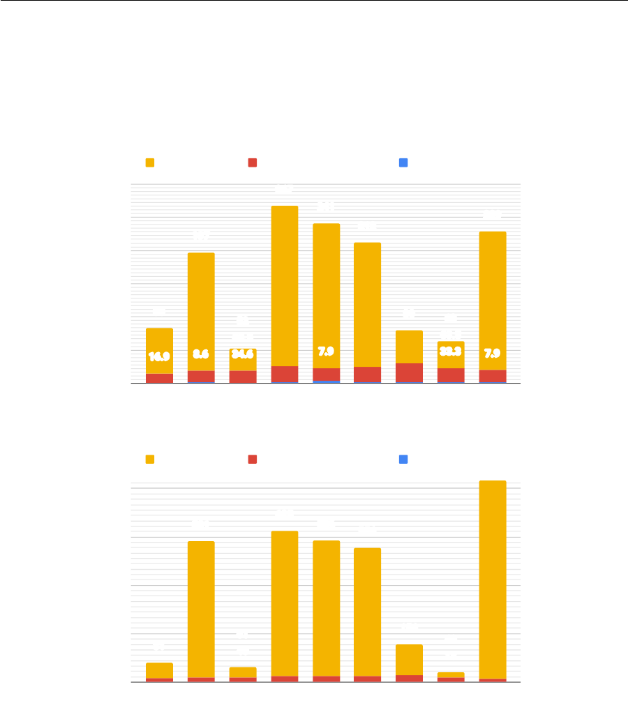
Chapter 8 Squerall Evaluation and Use Cases

16.9

8.6 34.6

9.0

7.9

10.8

35.0

33.3

7.9

81.9

90.4

63.5

90.3

90.5

88.2

62.5

63.5

91.3

197

267

241

212

229

100

150

200

250

300

Q1 Q2 Q3 Q4 Q5 Q6 Q7 Q8 Q10

Query Execution Relevant Source Detection Query Analysis

(a) Spark Scale 1.

520

624

560

575

134

818

581

625

586

556

156

832

200

400

600

800

Q1 Q2 Q3 Q4 Q5 Q6 Q7 Q8 Q10

Query Execution Relevant Source Detection Query Analysis

(b) Spark Scale 2.

Figure 8.1: Stacked view of the execution time phases on Presto (seconds). Bottom-up: Query Analyses,

Relevant Source Detection, and Query Execution, the sum of which is the total Execution Time shown

above the bars. Very low numbers are omitted for clarity.

116

8.1 Evaluation Over Syntactic Data

299

123

120

252

302

132

128

124

283

100

150

200

250

300

350

Q1 Q2 Q3 Q4 Q5 Q6 Q7 Q8 Q10

Query Execution Relevant Source Detection Query Analysis

(a) Presto Scale 1.

16.9

8.6 34.6

9.0

7.9

10.8

35.0

33.3

7.9

81.9

90.4

63.5

90.3

90.5

88.2

62.5

63.5

91.3

197

267

241

212

229

100

150

200

250

300

Q1 Q2 Q3 Q4 Q5 Q6 Q7 Q8 Q10

Query Execution Relevant Source Detection Query Analysis

(b) Presto Scale 2.

Figure 8.2: Stacked view of the execution time phases on Presto (seconds). Bottom-up: Query Analyses,

Relevant Source Detection, and Query Execution, the sum of which is the total Execution Time shown

above the bars. Very low numbers are omitted for clarity.

117

Chapter 8 Squerall Evaluation and Use Cases

100

200

300

Q1 Q2 Q3 Q4 Q5 Q6 Q7 Q8 Q10

Presto Spark

(a) Scale 1.

200

400

600

800

Q1 Q2 Q3 Q4 Q5 Q6 Q7 Q8 Q10

Presto Spark

(b) Scale 2.

500

1000

1500

2000

2500

Q1 Q2 Q3 Q4 Q5 Q6 Q7 Q8 Q10

Presto Spark

Figure 8.3: Query execution time (seconds). Comparing Spark-based vs. Presto-based Squerall.

118

8.1 Evaluation Over Syntactic Data

Performance

The columns in Figure 8.1 and Figure 8.2 show the query execution times divided into three

phases (each with distinct color):

1. Query Analysis:

Time taken to extract the stars, joins between stars, and the various

query operations linked to every star e.g., ﬁltering, ordering, aggregation, etc.

2. Relevant Source Detection:

Time taken to visit the mappings and ﬁnd relevant entities

by matching SPARQL star types and predicates against source entities and attributes.

3. Query Execution:

Time taken by the underlying engine (Spark or Presto) to eﬀectively

query the (relevant) data sources and collect the results. This includes loading the relevant

entities into ParSets (or a subset if ﬁlters are pushed down to the sources), performing

query operations e.g., ﬁltering, executing joins between ParSets, and ﬁnally performing

results-wide operations e.g., order, aggregate, limit, etc.

The results

presented in Figures 8.1, 8.2 and 8.3 suggest the following:

•

Presto-based Squarall is faster than Spark-based in most cases except for Q3 and Q10

at Scale 1. It has comparable to slightly lower performance in Q1 and Q8 at Scale 2.

This superiority can be explained by Presto’s nature that is precisely built and optimized

for running cross-source interactive SQL queries. Spark, on the other hand, is a general-

purpose engine with a SQL layer, which builds on Spark’s core in-memory structures that

are not originally designed for ad hoc querying. Unlike Spark, Presto does not load entities

in blocks but streams them through a query execution pipeline [208]. However, Presto’s

speed comes at the cost of weaker query resiliency. Spark, on the other hand, is more

optimized for fault tolerance and query recovery, making it more suitable for long-running

complex queries. The latter are, however, not the case of our benchmark queries. (Q1)

•

Query Analysis time is negligible; in all the cases it did not exceed 4 seconds, ranging

from < 1% to 8% of the total execution time. Relevant Source Detection time varies with

the query and scale. It ranges from 0.3% (Q3 Presto Scale 1) to 38.6% (Q8 Spark Scale 2).

It is, however, homogeneous across the queries of the same scale and query engine. Query

Execution time is what dominates the total query execution time in all the cases. It ranges

from %42.9 (Q8 Presto Scale 1) to 99% (Q3 Spark Scale 2), with most percentages being

about or above 90%, regardless of the total execution time. Both Query Analysis and

Relevant Source Detection depend on the query and not the data, so their performance is

not aﬀected by the data size (hence the absence of numbers for Scale 3). (Q2)

•

Increasing the size of the queried data did not deteriorate query performance. Co-relating

query time and data scale indicates that performance is proprietorial to data size. Besides,

all the queries ﬁnished within the threshold. (Q3)

•

The number of joins did not have a decisive impact on query performance, it rather should

be taken in combination with other factors, e.g., the size of involved data, the presence of

ﬁlters, etc. For example, Q2 joins only two data sources but has comparable performance

with Q5 and Q6 that join three data sources. This may be due to the presence of ﬁltering

in Q5 and Q6. Q7 and Q8 involve four data sources, yet they are among the fastest queries.

Also available online at:https://github.com/EIS-Bonn/Squerall/tree/master/evaluation

119

Chapter 8 Squerall Evaluation and Use Cases

Metrics Spark Presto

Node 1 Node 2 Node 3 Node 1 Node 2 Node 3

CPU Average (%) 4.327 7.141 4.327 2.283 2.858 2.283

Time Above 90% CPU (s) 9 71 9 0 2 0

Time Above 80% CPU (s) 19 119 19 0 5 0

Max Memory (GB) 98.4 100 98.4 99.5 99.7 99.5

Data Sent (GB) 4.5 6.3 4.5 5.4 8.5 5.4

Data Received (GB) 3.5 3.0 3.5 8.4 4.6 8.4

Data Read (GB) 9.6 5.6 9.6 1.9 0.2 1.9

Table 8.3: Resource Consumption by Spark and Presto across the three nodes on Scale 2.

This is because they involve the small entities Person and Producer, which signiﬁcantly

reduce the intermediate results to join. With four data sources, Q4 is among the most

expensive. This can be attributed to the fact that the ﬁlter on products is not selective

(

?p1 > 630

), in contrast to Q7 and Q8 (

?product = 9

). Although, the three-source join

Q10 involves the small entity Producer, it is the most expensive; this can be attributed to

the very unselective product ﬁlter it has (?product > 9). (Q4)

Resource Consumption

Resource consumption is visually represented in Figure 8.4 and reported in Table 8.3. We

recorded (1) CPU utilization by calculating its average percentage usage as well as the number

of times it reached 80% and 90%, (2) memory used in GB, (3) data sent across the network in

GB, and (4) data read from disk in GB. We make the following observations (Q5):

•

Although the average CPU is low (below 10%), monitoring the 90% and 80% spikes shows

that there were many instants where the CPU was almost fully used. The latter applies

to Spark only, as Presto had far less 80%, 90% and average CPU usage, making it a lot

less CPU-greedy than Spark.

•

From the CPU average, it still holds that the queries overall are not CPU-intensive. CPU

is in most of the time idle; the query time is rather used by the loading and transfer

(shuﬄing) of the data between the nodes.

•

The total memory reserved, 250GB per node, was not fully utilized; at most

≈

100GB was

used by both Spark and Presto.

•

Presto reads less data from disk (Data Read), which can be due to one of the following.

Presto does not read the data in full blocks but rather streams it through its execution

pipelines. Presto might also be more eﬀective at ﬁltering irrelevant data and already

starting query processing with reduced intermediate results.

Moreover, in Figure 8.4, we represent as a function of time the CPU utilization (in orange,

top), the memory usage (in dashed red, bottom) and the data sent over the network

(in light

blue, bottom) second by second during the complete run of the benchmark at Scale 2 with Spark.

The noticed curve stresses correspond to the nine evaluated queries. We notice the following:

For clarity reasons, we do not include Data Received traﬃc, since it is completely synchronized with Data Sent.

120

8.2 Evaluation Over Real-World Data

•

CPU utilization curves change simultaneously with Data Sent curve, which implies that

there is a constant data movement throughout query processing. Data movement is mainly

due to the join operation that exists in all queries.

•

Changes in all the three represented metrics are almost synchronized throughout all query

executions, e.g., there is no apparent delay between Data Sent or Memory usage and the

beginning of the CPU computation.

•

Memory activity is correlated with the data activities (received and sent), all changes in

memory usage levels are correlated with high network activity.

•

Unexpectedly, the memory usage seems to remain stable between two consecutive query

executions, which is in contradiction with our experimental protocol that applies cache

clearing between each query. In practice, this can be attributed to the fact that even if

some blocks of memory are freed, they remain shown as used as long as they are not used

again

8.2 Evaluation Over Real-World Data

Squerall has been evaluated internally in a large manufacturing industry

. An internal technology,

called Surface-Mount Technology, generates ﬁne-grained manufacturing data in a streaming

fashion and stores it in local log ﬁles. Consequently, the resulted size of the data is considerable.

Squerall is used to query this data joining distinct subsets thereof and computing aggregations

over time intervals. In this section, we ﬁrst describe the use case and technology involved, then

detail how Squerall is used, then ﬁnally report on its querying performance.

8.2.1 Use Case Description

Surface-Mount Technology, SMT, is a process for mounting electronic components, e.g., micro-

chips, resistors, capacitors, on print-circuit boards, PCBs. Several sub-processes are involved

in producing these PCBs and are executed by specialized machines. We are interested in two

sub-processes in particular: Surface Mount Devices, SMD, and Automatic Optical Inspection,

AOI. The SMD places the electronic components on top of the PCBs, and the AOI inspects

the boards for any error that could have occurred, e.g., misplaced or bad solder components.

To be able to improve the SMT process in general and the error detection process at the end

of the SMT line in particular, the semantics of the data generated by the machines should be

harmonized. This can be achieved by posing a semantic model that uniﬁes the interpretation

of the diﬀerent concepts. This allows to run ad hoc queries over the data generated by the

two sub-processes in a uniform way. SMT and AOI data is available in Parquet format, other

sub-processes generate data in CSV format, etc. In order to be able to access these heterogeneous

data sources uniformly, Squerall has been used.

The SMT use case has the following requirements that need to be met by the access solution,

which is Squerall in our case:

For more details, see following the common UNIX strategy of memory manage-

ment

https://git.kernel.org/pub/scm/linux/kernel/git/torvalds/linux.git/commit/?id=

34e431b0ae398fc54ea69ff85ec700722c9da773

We are abide by not revealing identity, data or ontology.

121

Chapter 8 Squerall Evaluation and Use Cases

200

400

600

800

1,000

1,200

1,400

1,600

1,800

2,000

2,200

2,400

2,600

2,800

3,000

3,200

3,400

100

CPU (%)

200

400

600

800

1,000

1,200

1,400

1,600

1,800

2,000

2,200

2,400

2,600

2,800

3,000

3,200

3,400

Time (seconds)

Data Sent (B)

0.4

0.5

0.6

0.7

0.8

0.9

·10

Memory (B)

Figure 8.4: Resource consumption recorded on one cluster node (which we observed was representative of

the other nodes) with Spark as query engine on Scale 2. Top is CPU percentage utilization. Bottom left

dashed is RAM (in Bytes) recorded at instant t, e.g., 0

4x10

B ≈

. Bottom right is Data Sent

across the network (in Bytes) at instant t, e.g., 10

B ≈ 95M B.

122

8.2 Evaluation Over Real-World Data

SMD Tables AOI Data Tables

Event aoiEvent

Machine aoiFailures

ProcessedPanel aoiProcessedPanel

ProcessedComponents aoiComponents

Feeder aoiComponentsPin

Nozzle aoiClassiﬁcations

smdBoard aoiMesLocation

Head

Table 8.4: SMD and AOI provided tables.

• R1.

Querying the data uniformly using SPARQL as query language exploiting data

semantics that is encoded in the SMT ontology.

• R2. Querying should be scalable accessing the various provided data sizes.

• R3.

Querying should support temporal queries (i.e.,

FILTER

on the time), and aggregation

queries (i.e. GROUP BY with aggregate functions, e.g., sum, average).

SMT-generated Data.

SMT use case data consists of ﬁfteen tables, eight pertaining to SMD

sub-process and seven to AOI sub-process (see Table 8.4). For SMT, Event is the action performed

(e.g. pick, place), Machine is the machine performing the action, ProcessedComponents are

the components being moved (e.g., picked, placed), Feeder is a device from which the machine

picks a component, ProcessedPanel and Board are respectively the panel and board where

components get placed, Head is the mechanical arm moving the component, Nozzle is the

end used to handle a speciﬁc type of component. For AOI, Event is the action during which

the failure happened, Failure is the failure speciﬁcation, Component and ProcessedPanel are

respectively which component and panel the failure concerns, MesLocation is the panel location,

and CompoenentstPin is the component connector on which the error was detected.

8.2.2 Squerall Usage

Thanks to Squerall’s internal abstraction component (ParSets), data in its format heterogeneity

can be represented and queried in a uniform manner. The target data of SMT use case is SMD

and AOI, which both being stored in Parquet format. As such, data itself is not heterogeneous by

nature, however, it beneﬁts from Squerall mediation mechanism that supports the simultaneous

access to multiple data sources. In other words, the query is run against the abstraction

layer regardless of where data was originated from; all data being of Parquet format or other

heterogeneous formats. The use case also principally beneﬁts from Squerall scalability at

querying large data sources, thanks to leveraging Big Data technologies. Limited to the available

infrastructure at the premises of the use case company, only Apache Spark is used and not

Presto.

As the data generated belongs to the same domain, the SMT use case does not require

query-time transformation (to enable joinability). Hence, we omit query-time transformations

from Squerall architecture and suggest a simpliﬁed version, which is presented in Figure 8.5.

To interact with Squerall, the user issues a query on the command line where the results are

123

Chapter 8 Squerall Evaluation and Use Cases

DF2

DF1 DF

Join

DataFrames

Filtered

DataFrames

Relevant

Data Sources

Distributed

Query

Processor

Filtering

Query

Decomposer

Mappings

Final Results

Data Wrapper

Relevant Entity

Extractor

Data Lake

Distributed

Execution

Environment

(DEE)

Union

DF1

Conﬁg

Query

Aggregate

and/or order

Figure 8.5: Squerall architecture variation excluding query-time transformations. ParSet is replaced by

its implementation in Spark, namely DataFrame.

subsequently shown, see Figure 8.6. The output returned in the console ﬁrst shows the query

that is being executed, then the schema of the results table, then the results table itself, then

the number of results and ﬁnally the time taken by the query execution.

8.2.3 Evaluation

In the following, we will report on the empirical study, which we have conducted to evaluate

Squerall’s performance querying SMT data. The research questions addressed are reduced to

the following:

• RQ1:

What is the performance of Spark-based Squerall accessing SMT data by means of

join, aggregation and temporal queries?

• RQ2:

What is the performance of Spark-based Squerall when increasing data sizes are

queried?

Data and queries

Three sizes of SMT data are used for the evaluation, as shown in Table 8.5. SMT use case involves

thirteen (13) queries, which have been evaluated using Squerall and reported in Table 8.6.

124

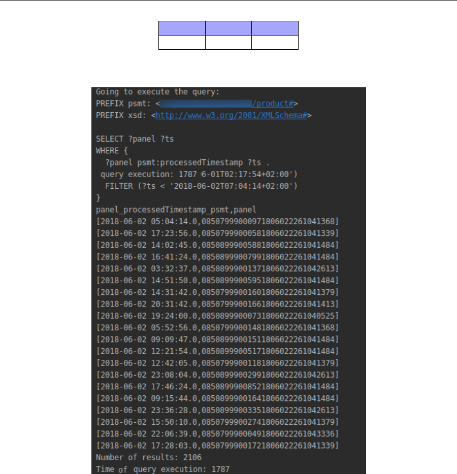
8.2 Evaluation Over Real-World Data

Scale 1 Scale 2 Scale 3

439M 3.8G 7.7G

Table 8.5: The sizes of the three data scales.

Figure 8.6: An example of the console output returned by Squerall running a query. It shows the issued

query then the results then the execution time (seconds).

Discussion

Table 8.6 shows all the queries, along with their support status (supported by Squerall or not),

their query execution time across the three data scales and a description of their content. All

queries ﬁnished within the threshold of 300 seconds (5 minutes) in the three data scales, with

no empty results set. Query times range from 0.25s minimum (Scale 1) to 129s maximum (Scale

3). Q1 and Q2 are the fastest queries; Q1 does not contain any join and ﬁlters the results to

only one day of data. Q2 contains two joins but the ﬁlter signiﬁcantly reduces the results to

one speciﬁc

panelId

. Q5 and Q13 are the slowest queries as they involve two joins including

both SMD and AOI data with no ﬁlter. Q13 is slower than Q5 with a factor of 2, as it does

125

Chapter 8 Squerall Evaluation and Use Cases

Query Supported? Scl 1 Scl 2 Scl 3 Description

Q1 1.28 2.15 2.02 No join, time ﬁlter

Q2 0.27 3.26 3.74 2 joins, ID ﬁlter

Q3 (sub-q) / / / /

Q4 (sub-q) / / / /

Q5 7.17 36.16 68.79 2 joins, SMT & AOI, ID ﬁlter

Q6 (sub-q) / / / /

Q7 (obj-obj join) / / / /

Q8 2.78 9.85 29.98 1 join, time ﬁlter

Q9 (agg sub) / / / /

Q10 2.98 4.74 5.38 1 join, SMD & AOI, time ﬁlter, agg.

Q11 4.68 5.34 11.77 2 joins, SMD & AOI, time ﬁlter, agg.

Q12 (agg sub) / / / /

Q13 14.51 79.52 129.59 2 joins, SMD & AOI

Table 8.6: Query Execution times (seconds). sub-q refers to a query containing a sub-query, obj-obj join

refers to a query that contains joins at the object position, and agg obj refers to a query that contains

an aggregation on the subject. Under Description, ’time ﬁlter’ means that the query contains ﬁlter

restricting the results inside a speciﬁc time interval, ’ID ﬁlter’ means that the query contains a ﬁlter on a

very speciﬁc panelID.

not contain any ﬁlter in contrast to Q5. Q10 and Q11 both involve join plus an aggregation,

however, they are relatively fast as they involve ﬁltering on a timestamp ﬁeld limiting the results

to only ten days worth of data. Q11 is slower than Q10 as it joins between three tables in

contrast to two in Q10. Finally, Q8 falls in the middle of the query time range; although it

contains a join, it ﬁlters the results to one day worth of data.

Table 8.6 also points to what queries are not supported. Squerall at the time of conducting

the evaluation did not support SPARQL queries containing a sub-query, an object to object

join, a ﬁlter between object variables, and aggregation on the subject position. See Figure 8.7

for unsupported query examples and explanations. This aﬀects Q3 and Q6 (sub-query), Q7 and

Q4 (object-object join), and Q9 and Q12 (aggregation on the subject position). When there is a

ﬁlter comparing two object variables, the case of Q2 and Q4, the query is executed with the

unsupported ﬁlter omitted.

8.3 Summary

In this chapter, we reported on our experience evaluating Squerall performance using both

synthetic and real-world use cases. In the synthetic use case, we used Berlin Benchmark, both

data and query. We used a subset of the data (tables) to populate the data sources that Squerall

supports. We also used a subset of the queries (nine out of twelve) excluding unsupported query

types (e.g.,

DESCRIBE

). We evaluated Squerall accuracy, performance and query execution time

breakdown into sub-phases: query analysis, relevant source detection and query execution. The

results suggested that all queries exhibited 100% accuracy and that all queries were successful

ﬁnishing within the threshold. The results also showed that query execution time was in the

worst case proportional to the increasing data sizes. In the real-world use case, Squerall executed

126

8.3 Summary

?f fsmt:isFailureOf ?pin ;

fsmt:failureType ?type .

?c psmt:hasPin ?pin .

psmt:referenceDesignator ?r .

psmt:hasSMDHead ?h .

(a) An example of object-object join from Q7 on variable ?pin between the two stars ?f and ?c.

SELECT (COUNT(?failure) as ?failuresShape) ?shape

WHERE {

?component psmt:hasPin ?pin ;

psmt:componentShape ?shape .

?failure a fsmt:Tombstoning ;

fsmt:isFailureOf ?pin .

(b) An example of aggregation on object from Q12, COUNT on ?failure object variable.

FILTER (?ts2 > ?ts)

FILTER (?panelId = "08507999002521806222261041592")

Figure 8.7: Examples of unsupported SPARQL queries. The red font color highlights the unsupported

operations. In (a) object-object join, in (b) aggregation on the abject variable, (c) ﬁlter including two

variables. Queries (a) and (b) are discarded, query (c) is executed excluding the unsupported ﬁlter

(strikethrough).

queries withing the threshold of ﬁve minutes along the three data sizes used. The use case

included queries with unsupported SPARQL constructs e.g., sub-queries, in which case the

queries were not executed. Supporting this constructs is planned for Squerall’s next release.

127

CHAPTER 9

Conclusion

"A person who never made a mistake

never tried anything new."

Albert Einstein

In this thesis, we investigated the problem of providing an ad hoc uniform access to large and

heterogeneous data sources using Semantic Web techniques and technologies. We examined the

applicability of existing Semantic-based Data Integration principles, notably, Ontology-Based

Data Access, to the Big Data Management technology space. We studied both the Physical

and Logical approaches of Data Integration, with more emphasis on the latter. We deﬁned the

tackled problem, challenges and contributions in Chapter 1. We presented the background and

the necessary preliminaries in Chapter 2. We gave a state-of-the-art overview of the related

eﬀorts in Chapter 3. As model and query conversion was an integral part of our envisioned Data

Integration approaches, we conducted a survey on the Query Translation approaches, reported

in Chapter 4. The survey also supported us in the diﬀerent design and optimization decisions

we have made. Chapter 5 was dedicated to describing our Physical Data Integration approach,

including the Semantiﬁed Big Data Architecture deﬁnition, its requirements, implementation

and empirical evaluation. Chapter 6 was dedicated to describing our Logical Data Integration

approach, including the Semantic Data Lake deﬁnition, its architecture as well as a set of

requirements for its implementation. Our implementation of the Semantic Data Lake was

detailed in Chapter 7. Finally, Chapter 8 presented two use cases of the latter implementation,

one based on a synthetic benchmark and one based on a real-world industrial application.

9.1 Revisiting the Research Questions

In the introduction of the thesis (Chapter 1), we have deﬁned four research questions that

were intended to frame our core contributions of the thesis. In this conclusion, it is important

to retrospectively revisit every research question and make a brief summary about how it

was tackled. In particular, how our Physical and Logical approaches for Data Integration of

heterogeneous and large data sources were conceptually deﬁned and practically implemented.

RQ1.

What are the criteria that lead to deciding which query language can be most

suitable as the basis for Data Integration?

129

Chapter 9 Conclusion

We have tackled this question by conducting an extensive literature review on the topic of

Query Translation, reported in Chapter 4. As the topic was of a general interest and pertained

to an essential aspect of data retrieval in general, the review was enriching and proﬁtable. It

covered both the syntactic and semantic considerations of query translation, query rewriting

and optimization, and the diﬀerent strategies of transitioning from an input to a target query,

e.g., direct, via intermediate phase, using an (abstract) meta-language, etc. The survey had

several motivations, summarized as follows. First, as model and query conversion is at the

core of data integration, it was necessary to have a general overview of the existing query

translation approaches. This helped us support the choices we made for the external query

language (SPARQL), underlying meta query language (SQL), as well as the transition between

the two in a query execution middleware. For example, SPARQL and SQL were the most

translated to and from query languages, which makes them very suitable to act as a universal

query language. Second, the feasibility and eﬃciency of a query translation method can only be

evaluated within an operable data translation or migration system, which we wanted to leverage

to make sound design decisions in our diﬀerent integration approaches. As examples, the use of a

meta-language, as well as query augmentation starting from iteratively analyzing the input query

were both prevalent techniques from the literature, which we adopted. A side motivation was

that, at the time of reviewing, there was no published survey addressing the query translation

across multiple query languages. All that existed was aiming at pair-wise methods involving

only two query languages. We reviewed more than forty query translation eﬀorts, including tools

only available in source hosting services with accompanying description. The survey allowed us

to detect patterns and criteria, against which we classiﬁed the reviewed eﬀorts. The criteria

included translation type (direct, indirect), schema-aware or mappings-dependent translation,

commonly used optimization techniques, query coverage as well as community adoption. Finally,

through the survey, we were able to detect the translation paths for which there existed a few

to no publications, as well as to learn some lessons for future research on the topic.

RQ2.

Do Semantic Technologies provide ground and strategies for solving Physical

Integration in the context of Big Data Management i.e., techniques for the representation,

storage and uniform querying of large and heterogeneous data sources?

This question was addressed by the Semantic-based Physical Data Integration, detailed in

Chapter 5. In the presence of heterogeneous data sources, classiﬁed as semantic and non-

semantic, the aim was to access the data in a uniform way. First, we suggested a generic

blueprint called SBDA, for Semantiﬁed Big Data Architecture, that supports the integration of

hybrid semantic and non-semantic data, and the access to the integrated data. The architecture

leveraged Semantic Web techniques and technologies, such as the RDF data model and SPARQL

query language. RDF was used as the underlying data model under which all input data of

diﬀerent types is represented and physically converted. Data is then naturally queried in a

uniform way using SPARQL. As we target the integration of large datasets, we proposed a

data model and storage that is both space-eﬃcient and scalable, i.e., accommodating increasing

data sizes while keeping reasonable query performance. We suggested a partitioning scheme

that is based on the popular Property Table under which RDF instances are stored into tables

containing columns corresponding to the instance predicates, e.g., ﬁrst name, last name and

birth date of a person. The tables are clustered by type (RDF class), where all instances of the

same type are stored in the same dedicated table. Further, multi-typed instances are captured

within the same table via incorporating an extra column storing a list of all types that the

130

9.1 Revisiting the Research Questions

instance belongs to. The table also contains a column for every detected other type, which

indicates whether or not (ﬂag) an instance is also of that type. At the physical level, the tables

are stored in a columnar-format where data is organized by columns instead of rows. This

organization makes it very eﬃcient to store tuples of a large number of columns while accessing

only a subset of them. It also enables eﬃcient compression as the data of the same column

is homogeneous. These characteristics make this format particularly useful for storing RDF

data under our scheme. A SPARQL query typically involves only a subset of the instance

predicates. We also beneﬁt from the compression eﬃciency as we target the integration of large

datasets. Under this data partitioning and clustering scheme, input SPARQL query needs to

be transparently rewritten to involve the other tables where instances of the same type can be

found. A proof-of-concept implementation of the architecture was presented and evaluated for

performance and generated data size. Both semantic data (RDF) and non-semantic data (XML)

were integrated and queried. In particular, the implementation was compared against a popular

RDF triple store and showed its superiority in terms of space usage and query performance when

queries large data. State-of-the-art Big Data technologies, namely Apache Spark (ingestion and

querying) and Parquet (columnar storage) were used.

RQ3.

Can Semantic Technologies be used to incorporate an intermediate middleware

that allows to uniformly access original large and heterogeneous data sources on demand?

This question was addressed by the Semantic-based Logical Data Integration, detailed in

Chapter 6. Conversely to the Physical Integration, the aim here was to query the original data

sources, without a prior transformation to a unique model. In this case, the complexity is

shifted from the data ingestion to query processing. Given a query, it is required to detect the

relevant data sources, retrieve the intermediate results and combine them to form the ﬁnal query

answer. We proposed an architecture called SDL, for Semantic Data Lake, which is based on

the OBDA (Ontology-based Data Access) principles. We suggested a set of requirements that

should be met when implementing the SDL. For example, the implementation should execute

the queries, including multi-source joins, in a distributed manner to cope with data volume.

In SDL, data schemata (organized into entities and attributes) are mapped to ontology terms

(classes and predicates) creating a virtual semantic middleware against which SPARQL queries

can uniformly be posed. The input query is analyzed to extract all the triple pattern groups

that share the same subject. Additionally, the connections between these groups as well as any

involved query operations (e.g., sorting, grouping, solution modiﬁers) are detected. The triple

pattern predicates, assumed bound, are matched against the mappings to ﬁnd the entities that

have attributes matching every predicate. In distributed large-scale settings, two strategies of

accessing the detected relevant data entities were described. In the ﬁrst, the entities are loaded

into distributed data structures that can be manipulated by the user. The data structures can

be joined following the triple pattern group connections. As optimization, predicate push-down

is applied to ﬁlter the entity at the data source level. The second strategy is when the SPARQL

query is internally converted into an intermediate query language, e.g., SQL. The intermediate

query is constructed in augmentation steps, by analyzing the input query (SPARQL). Once fully

constructed, the query is submitted to a query engine that accesses the relevant entities. We

presented an extensible implementation of the SDL, which uses RML and FnO for the mappings

and Apache Spark and Presto for query execution. The two engines provide the data structures

required to distribute the query processing, as well as many readily usable wrappers to enable

the loading of data into their internal data structures. The implementation is built following a

131

Chapter 9 Conclusion

modular design allowing it to be extended to support more data sources and incorporate new

query engines. The implementation is detailed in a dedicated Chapter 7.

RQ4.

Can Virtual Semantic Data Integration principles and their implementation be

applied to both synthetic and real-world use cases?

Our SDL implementation was evaluated in two use cases based respectively on a synthetic

benchmark and a real-world application from the Industry 4.0 domain. We described the

evaluation framework and presented the results in Chapter 8. In the synthetic use case, we

used the Berlin Benchmark, BSBM. We generated ﬁve datasets and loaded them into the ﬁve

supported data sources: MongoDB, Cassandra, Parquet CSV, and MySQL. We adapted ten

queries to use only the data we ingested and the supported SPARQL fragment. The queries

have various numbers of joins, to which we paid special attention to assess the eﬀect of joining

multiple heterogeneous data sources. We reported on the query execution time, broken down

into query analysis, relevant source detection and actual query execution time. We also examined

the implementation scalability by running the queries against three increasing data scales. We

reported on the query evaluation by, ﬁrst, comparing the results cardinality against the results

of loading and querying the same benchmark data into MySQL. For data sizes that are beyond

MySQL limits, we resorted to comparing the cardinality when Spark and Presto are used as

query engines. For the industrial use case, we have experimented with real-world data generated

using a so-called Surface-Mount Technology. To evaluate the query performance and scalability,

we ran the queries against three data scales. The use case involved thirteen SPARQL queries,

which we ran and reported. Some queries involved unsupported constructs e.g., sub-queries and

aggregation on the object position.

9.2 Limitations and Future Work

Data Integration poses challenges at various levels, from query analysis to data extraction

to results reconciliation and representation. Thus, there are several avenues for improvement

as well as for extending the current state of the work. In the following, we list a number of

directions that the current work could take in the future, classiﬁed into Semantic-based Physical

Integration and Semantic-based Logical Integration.

9.2.1 Semantic-based Physical Integration

Optimizing the Data Ingestion

In the Semantic-based Physical Integration, we focused our eﬀort more on providing data model

and storage schemes that support the integration of large amounts of data under the RDF

standard. The most signiﬁcant lesson learned was that the ingestion of the heterogeneous

datasets under a chosen partitioning scheme is a laborious and costly task. The cost increases

with the complexity of the partition scheme used. When we assume the absence of an RDF

schema, which is not uncommon, the ingestion of RDF data requires exhaustively processing

data triple by triple. With large RDF data, this operation becomes severely resource and

time-consuming. Most of the existing work that we have reviewed had also incorporated a

heavy data ingestion phase in order to pre-compute various joins optimizing for diﬀerent query

shapes and patterns. However, it is usually understated that the improved results were only

132

9.2 Limitations and Future Work

possible due to an intensive data ingestion phase, thus little to no attention was dedicated to its

optimization. While we recognize the value of collecting statistics, indexing and partitioning the

data during the loading time, we deem that a heavy data ingestion phase should be addressed

with adequate optimization techniques. The problem is more apparent in our context of large-

scale data-intensive environments. For example, statistics calculations could be done in a lazy

fashion after data has been loaded. Data indexing can also be performed in a similar fashion. In

distributed systems, the notion of eventual consistency [216] can be ported to having eventual

statistics or eventual indexing. With this, the ﬁrst queries may be slow but future runs of

the same or other queries will eventually have an improved execution time. Data partitioning

can also become challenging. If the data has to undergo fundamental model conversion or

signiﬁcant data transformation or adaptation, partitioning optimization possibilities become

limited. One may beneﬁt from applying traditional partitioning and scheduling algorithms at

the data ingestion phase, e.g., Range partitioning, Hash partitioning, List partitioning, etc.

For example, distributing RDF triples into compute nodes based on RDF subject or property.

The latter can be useful for Vertical Partitioning schemes. However, this requires a deeper

level of customization, which is not always evident if an existing processing engine is used,

e.g. Hadoop MapReduce, Spark. In this regard, it is not always recommended to manipulate

the underlying distribution primitives and data structures, as this may possibly conﬂict with

the default ingestion and optimization strategies. For example in Hadoop MapReduce, a

dedicated programming interface called

Partitioner

oﬀers the possibility to impose a custom

data distribution across the cluster nodes. Exploring these avenues is a viable future next-step

for this thesis.

Expanding the Scope of Query Patterns

Our suggested Class-based Multi-Type-Aware Property Table scheme has some drawbacks. First,

it not allow to answer SPARQL queries where the predicate is unbound. Although it has been

reported that unbound predicates are uncommon in SPARQL queries [54], it is still a valid

extension of the current querying coverage. This could be implemented by additionally storing

the data under the Triple Table scheme (subject, predicate, object). This, however, would add to

both the data ingestion time and ingested data size. However, we could use the same columnar

format (Parquet) to store this table and thus beneﬁt from its eﬃcient compression capability.

Incorporating Provenance Retention

In a Physical Integration environment, it comes naturally to think of incorporating provenance

retention both at the data and query level. Provenance information includes the original source

from which a data item was retrieved, the time of retrieval, the person or agent retrieving the

information, the sources involved in the query results, the person or agent issuing the query, the

query execution time, etc. At the data level, since the data ingestion is a supervised operation,

one can easily record, for each ingested item, which data source it was retrieved from, when and

by whom. For example, while ingesting RDF triples, it is possible to capture the provenance

information at the triple level. It can accompany the triple itself, e.g., (triple, source, time, user),

or similarly if other partitioning schemes are used e.g., in Predicate-based Vertical Partitioning

(subject, object, source, time, user). Provenance information can also be saved in form of an

auxiliary index where every triple is assigned an identiﬁer (e.g., based on a hash function)

and mapped to the provenance information e.g., e.g., (recordID, source, time, user). An RDF

133

Chapter 9 Conclusion

technique called reiﬁcation could alternatively be used, whereby provenance information is

encoded in the form of RDF statements about RDF statements.

At the query level, it is particularly important to record the query execution time and

cardinality. This allows following how the results to the same query evolve over time. The

results are timestamped once obtained and saved along with the query statement, the person or

agent issuing the query, etc. If provenance information is attached to individual data elements,

the query engine can automatically retrieve the provenance information along with the query

results. Alternatively, a hash map can be populated during data ingestion, so it is possible to

ﬁnd the original data source by mapping data elements appearing in the results. Technically,

distributed Key-value in-memory stores (e.g., Redis

) can be used to implement these hash maps.

As the provenance information can escalate in size, such distributed Key-value stores can also be

leveraged to optimize for disk usage by sharding (dividing) the provenance data across multiple

nodes. Finally, Specialized provenance ontologies (e.g., W3C recommendation PROV-O [217])

accompanied with data catalog ontologies (e.g., W3C recommendation DCAT [218]) can be

used to capture provenance information in the RDF model.

Diversifying Query Results Representation

The default SPARQL query answer is tabular, where every column corresponds to the projected

RDF variable. However, when the query is of analytical nature, i.e., computing statistics using

aggregation functions (

MAX

MIN

AVG

, etc.), the query results can also be represented using the

W3C recommended Data Cube vocabulary [219]. In addition to enabling interoperability and

contributing statistical RDF data that can be linked to or from, results can also be visualized

using specialized tools e.g., CubeViz [220]

. Consider the query "Give me the number of buses

per region and driver gender", each aggregation column (region and gender) corresponds to a

dimension, the column of the computed statistical value (bus_number) is the measure, and

the computed values themselves are the observations. Exposing various result formats is also a

natural extension of the current Data Integration work.

9.2.2 Semantic-based Logical Integration

Supporting a Larger SPARQL Fragment

The SPARQL fragment that our SDL implementation, Squerall, supports has evolved thanks

to the projects it was used in (raised by SANSA users and the I4.0 use case). However, there

are still a few query patterns and operations that we ﬁnd important to cover in the future.

For example, sub-queries were common in the industrial use case we described in Chapter 8.

Object-object join and aggregation on object variables were also requested. We also see

UNION

and

OPTIONAL

frequently discussed in the literature. While supporting nested sub-queries is

challenging given that we map every query star to a ParSet (implemented in tabular format),

the other features can be relatively straightforwardly addressed. In other words, the addressable

operations and constructs are those that do not interfere with our start-to-ParSet principle. In

our tabular-based implementation, this requirement is translated to keeping the query shape

ﬂat. For example,

UNION

can be addressable because it just requires combining two separate

entities, and both our used engines Spark and Presto support an equivalent

UNION

operation.

https://redis.io

https://github.com/AKSW/cubeviz.ontowiki

134

9.2 Limitations and Future Work

OPTIONAL

was less common in the use cases we were involved in, but it is generally translated to

SQL LEFT OUTER JOIN. It is noteworthy, however, that we did not envision Squerall to be or

become a fully-ﬂedged RDF store. The use of SPARQL was more motivated by bridging between

the query and the heterogeneous data sources, passing by the mappings. RDF-speciﬁc query

operations and types such as blank nodes, named graphs, isURI, isLiteral,

ASK

CONSTRUCT

, etc.

are considered out-of-the-scope.

Improving Extensibility

Reﬂected in both our suggested SDL architecture and our implementation of the architecture,

we paid special attention to allowing for extension opportunities. In Squerall, we showcased

how it can (programmatically) be extended to support more data sources and use other query

engines along with the currently-used Spark and Presto. In the ﬁrst extensibility aspect, our

current work advocated for the reuse of data source wrappers from the existing underlying query

engines, and thus avoid to each time reinvent the wheel as noticed in the literature. Not only

creating wrappers is a laborious error-prone task, it was also observed in several eﬀorts that

the wrappers were limited in their ability to match data from the source to the data structure

of the query engine. We had our own experience creating wrappers, e.g. MongoDB, and we

faced similar diﬃculties. However, it is remained to state that there might well be other sources

for which no wrapper exists. This means that the support for source heterogeneity of our

default implementation is limited by the number of wrappers the adopted query engine supports.

Although we demonstrated in this thesis the extensibility methodology for supporting new data

sources (applied to RDF data), it is still an important manual work involvement, which we aim

to partially alleviate by providing specialized guiding user interfaces and suggesting a set of

best practices.

The second extensibility aspect is adding another query engine. In subsection 6.2.2 we

showed that data can be queried either by manipulating ParSets or augmenting a self-contained

internal query submitted as-is to the underlying query engine. The former strategy requires the

implementation of common programmatic interfaces. As previously, programmatic challenges

can be alleviated by providing graphical interfaces or recommended best practices. The latter

strategy, on the other hand, has an intrinsic characteristic that can be levered to support more

query engines straightforwardly. That is accepting self-contained queries not requiring any

programmatic work. There exist other SQL query engines that can be interacted with using

this strategy e.g., Drill, Dremio, Impala. In the future, we can extend our implementation to all

these query engines using the exact same methods we have established for submitting queries to

Presto. These methods generate a self-contained query, which can be submitted as-is to the

other SQL query engines.

Comparing our SDL Implementation and Establishing an SDL Benchmark

We have not conducted any comparative evaluation against related eﬀorts. We rather self-

compared our strategies when both Spark and Presto are used. While we had interesting

results for the community, not comparing to another related eﬀort limits the value delivered by

the conducted evaluation. In fact, there was no existing SDL implementation or similar that

supported all or most of our supported sources. We found only two related eﬀorts both of which

supported a few data sources having only one data source in common with our implementation.

Eﬀorts for providing a SQL interface on top of NoSQL stores were also either limited in terms

135

Chapter 9 Conclusion

of data sources supported or lack crucial query operations like join. We will continue reviewing

the literature for any similar comparable work published. Alternatively, we might alter our

benchmarking framework as to compare against single-source approaches (thus eliminating

joins), or against SQL-based approaches by creating equivalent SQL queries to our SPARQL

queries. Nonetheless, this would not be a valuable comparison for the community and the results

would not advance the topic of the work in any signiﬁcant way.

On the other hand, there is still no benchmark dedicated to comparing SDL implementations.

Such a benchmark should be able to generate data that can be loaded into various heterogeneous

data sources and generate a set of SPARQL queries. The data can be generated in a canonical

format, e.g., relational, which can be saved into the diﬀerent heterogeneous data sources. This

can be achieved by leveraging the wrappers of existing distributed query engines, e.g., Spark.

This is the method we have followed to generate BSBM relational data (SQL dumps) and save

it into Cassandra, MongoDB, Parquet, CSV and MySQL. This method is straightforward and

can exploit the available wrappers of dozens of data source types. The benchmark should also

generate a set of mappings linking data schemata elements to ontology terms. The latter could

be user-deﬁned as they could be exemplary, which users can later adjust.

9.3 Closing Remark

In the scope of modern Big Data technologies, the topic of Semantic Data Integration, especially

the Virtual Integration, is still in its infancy. At the time of writing, there is no production-ready

openly-available solution that can be used for real-world use cases. For example, as mentioned

previously, the eﬀorts that are embarking on this domain lack a common ground that would allow

them to be evenly compared. This can also be attributed to the high dynamicity of many of these

systems that makes it very challenging to provide sustainable access mechanisms. To the same

argument, the substantial model diﬀerences between many of the so-called NoSQL stores makes it

virtually impossible to establish a standardized way to interface with these stores. This is a widely

recognized issue that is a source of active ongoing research. Moreover, from our own experience

during this thesis work, dealing with these modern storage and data management systems is a

technically tedious task involving a lot of trial-and-error due to the lack of documentation and

suﬃcient previous experiences. On the other hand, adopting the traditional OBDA systems

may seem a reasonable direction given their maturity in processing RDF data and dealing with

SPARQL speciﬁcities. However, Big Data has come with fundamentally diﬀerent semantics and

assumptions that would deeply alter the architecture of these traditional centralized OBDA

systems. These range from dealing with large distributed data requiring parallel processing

(e.g. distributed join) to supporting data sources that are very dissimilar in terms of their data

model, query syntax and access modality.

The Physical and Logical Data Integration are two diﬀerent approaches, which are also

opposite in certain respects. They both have their application scope, merits and challenges. The

Physical Data Integration is favored when it is explicitly desired to transform all input data into

a unique data model and, thus, beneﬁt from model uniformity advantages, e.g. improved query

performance. However, data transformation and centralization is a challenge that worsens with

the increased data volume and variety. The Logical Data Integration is favored if data freshness

and originality are not to be compromised. However, disparate data needs to be individually

accessed then, on-the-ﬂy, homogenized and reconciled. This lowers the time-to-query (i.e., data

is accessed directly) but raises the time-to-results (i.e., longer execution time). Our focus on the

136

9.3 Closing Remark

Logical Data Integration in this thesis gives no recommendation for the latter over the former.

It is a choice that we made after balancing between the technical challenge (a one that promises

faster progress based on our practical experience) and scientiﬁc impact and signiﬁcance (a one

that is more recent and, thus, with more open issues and innovation opportunities).

In the end, it is our hope that this thesis will serve as a reference for future students and

researchers in the topic of ‘Semantic Web for Big Data Integration’, setting foundations for

future research and development in the topic.

137

Bibliography

[1] D. Laney, Deja VVVu: others claiming Gartner’s construct for big data,

Gartner Blog, Jan 14 (2012) (cit. on p. 1).

[2] E. F. Codd, A relational model of data for large shared data banks,

Communications of the ACM 13 (1970) 377 (cit. on pp. 1, 42).

[3] S. Baškarada and A. Koronios, Unicorn data scientist: the rarest of breeds,

Program (2017).

[4] J. Dixon, Pentaho, Hadoop, and Data Lakes, Online; accessed 27-January-2019, 2010,

url: https://jamesdixon.wordpress.com/2010/10/14/pentaho-hadoop-and-data-

lakes (cit. on pp. 22, 42, 84, 85).

[5] D. Borthakur et al., HDFS architecture guide, Hadoop Apache Project 53 (2008) 2

(cit. on pp. 3, 18).

[6] O. Lassila, R. R. Swick et al.,

Resource description framework (RDF) model and syntax speciﬁcation, (1998)

(cit. on pp. 6, 14, 87).

[7] E. Prud’hommeaux and A. Seaborne, SPARQL Query Language for RDF,

W3C Recommentation, W3C, 2008, url:

http://www.w3.org/TR/rdf-sparql-query/

(cit. on pp. 6, 16).

[8] A. Poggi, D. Lembo, D. Calvanese, G. De Giacomo, M. Lenzerini and R. Rosati,

“Linking data to ontologies”, Journal on Data Semantics X, Springer, 2008

(cit. on pp. 8, 16, 25, 45, 85).

[9]

T. J. Berners-Lee, Information management: A proposal, tech. rep., 1989 (cit. on p. 13).

[10] J. Conklin, Hypertext: An introduction and survey, computer (1987) 17 (cit. on p. 13).

[11] T. J. Berners-Lee and R. Cailliau, WorldWideWeb: Proposal for a HyperText project,

(1990) (cit. on p. 13).

[12] T. Berners-Lee, J. Hendler, O. Lassila et al., The semantic web,

Scientiﬁc american 284 (2001) 28 (cit. on p. 13).

[13] M. Arenas, C. Gutierrez and J. Pérez, “Foundations of RDF databases”,

Reasoning Web International Summer School, Springer, 2009 158 (cit. on p. 14).

[14] T. Berners-Lee, R. Fielding, L. Masinter et al.,

Uniform resource identiﬁers (URI): Generic syntax, 1998 (cit. on p. 15).

[15] D. Fensel, “Ontologies”, Ontologies, Springer, 2001 11 (cit. on p. 15).

[16] M. Uschold and M. Gruninger, Ontologies: Principles, methods and applications,

The knowledge engineering review 11 (1996) 93 (cit. on p. 15).

139

Bibliography

[17] P. Agarwal, Ontological considerations in GIScience,

International Journal of Geographical Information Science

(2005) 501 (cit. on p. 15).

[18] T. Berners-Lee, Linked data-design issues,

http://www. w3. org/DesignIssues/LinkedData. html (2006) (cit. on p. 16).

[19] N. Guarino, D. Oberle and S. Staab, “What is an ontology?”, Handbook on ontologies,

Springer, 2009 1 (cit. on p. 16).

[20] J. Bailey, F. Bry, T. Furche and S. Schaﬀert,

“Web and semantic web query languages: A survey”,

Proceedings of the First international conference on Reasoning Web,

Springer-Verlag, 2005 35 (cit. on p. 16).

[21] P. Haase, J. Broekstra, A. Eberhart and R. Volz,

“A comparison of RDF query languages”, International Semantic Web Conference,

Springer, 2004 502 (cit. on pp. 16, 47).

[22] E. Prud’hommeaux and A. Seaborne, eds.,

SPARQL Query Language for RDF, W3C Recommendation, 2008,

url: http://www.w3.org/TR/rdf-sparql-query/ (cit. on p. 16).

[23] J. Pérez, M. Arenas and C. Gutierrez, Semantics and complexity of SPARQL,

ACM Transactions on Database Systems (TODS) 34 (2009) 16 (cit. on pp. 16, 43).

[24] J. P. Fry, S. Bramson, D. C. Fried, W. P. Grabowsky and J. Jeﬀries Jr,

Data management systems survey, tech. rep., MITRE CORP MCLEAN VA, 1969

(cit. on p. 17).

[25] J. P. Fry and E. H. Sibley, Evolution of data-base management systems,

ACM Computing Surveys (CSUR) 8 (1976) 7 (cit. on p. 17).

[26] F. Almeida and C. Calistru, The main challenges and issues of big data management,

International Journal of Research Studies in Computing 2 (2013) 11 (cit. on p. 17).

[27] J. Chen, Y. Chen, X. Du, C. Li, J. Lu, S. Zhao and X. Zhou,

Big data challenge: a data management perspective,

Frontiers of Computer Science 7 (2013) 157 (cit. on p. 17).

[28] M. Xiaofeng and C. Xiang,

Big data management: concepts, techniques and challenges [J],

Journal of computer research and development 1 (2013) 146 (cit. on p. 17).

[29] A. Siddiqa, I. A. T. Hashem, I. Yaqoob, M. Marjani, S. Shamshirband, A. Gani and

F. Nasaruddin, A survey of big data management: Taxonomy and state-of-the-art,

Journal of Network and Computer Applications 71 (2016) 151 (cit. on p. 17).

[30] D. D. Chamberlin and R. F. Boyce, “SEQUEL: A structured English query language”,

Proceedings of the 1974 ACM SIGFIDET (now SIGMOD) workshop on Data description,

access and control, ACM, 1974 249 (cit. on pp. 18, 42, 43, 63).

[31] T. J. W. I. R. C. R. Division and G. Denny,

An introduction to SQL, a structured query language, 1977 (cit. on p. 18).

[32]

J. Gray et al., “The transaction concept: Virtues and limitations”, VLDB, vol. 81, 1981

144 (cit. on p. 18).

140

[33] T. Haerder and A. Reuter, Principles of transaction-oriented database recovery,

ACM computing surveys (CSUR) 15 (1983) 287 (cit. on p. 18).

[34] T. White, Hadoop: The deﬁnitive guide, " O’Reilly Media, Inc.", 2012

(cit. on pp. 18, 26).

[35] E. Hewitt, Cassandra: the deﬁnitive guide, " O’Reilly Media, Inc.", 2010 (cit. on p. 19).

[36] A. H. Team, Apache HBase reference guide, Apache, version 2 (2016) (cit. on p. 19).

[37] C. Gormley and Z. Tong,

Elasticsearch: the deﬁnitive guide: a distributed real-time search and analytics engine,

" O’Reilly Media, Inc.", 2015 (cit. on p. 19).

[38] J. Dean and S. Ghemawat, MapReduce: simpliﬁed data processing on large clusters,

Communications of the ACM 51 (2008) 107 (cit. on p. 19).

[39] P. Carbone, A. Katsifodimos, S. Ewen, V. Markl, S. Haridi and K. Tzoumas,

Apache ﬂink: Stream and batch processing in a single engine, Bulletin of the IEEE

Computer Society Technical Committee on Data Engineering 36 (2015) (cit. on p. 19).

[40] M. Zaharia, M. Chowdhury, M. J. Franklin, S. Shenker and I. Stoica,

Spark: Cluster computing with working sets, HotCloud 10 (2010) 95

(cit. on pp. 19, 86, 98).

[41] D. Pritchett, Base: An acid alternative, Queue 6 (2008) 48 (cit. on p. 20).

[42] E. Hewitt, Cassandra: the deﬁnitive guide, " O’Reilly Media, Inc.", 2010 (cit. on p. 22).

[43] P. J. Sadalage and M. Fowler,

NoSQL distilled: a brief guide to the emerging world of polyglot persistence,

Pearson Education, 2013 (cit. on pp. 22, 42).

[44] M. Lenzerini, “Data integration: A theoretical perspective”,

Proceedings of the twenty-ﬁrst ACM SIGMOD-SIGACT-SIGART symposium on

Principles of database systems, ACM, 2002 233 (cit. on p. 23).

[45] G. Wiederhold, Mediators in the architecture of future information systems,

Computer 25 (1992) 38 (cit. on p. 24).

[46] M. J. Carey, L. M. Haas, P. M. Schwarz, M. Arya, W. F. Cody, R. Fagin, M. Flickner,

A. W. Luniewski, W. Niblack, D. Petkovic et al.,

“Towards heterogeneous multimedia information systems: The Garlic approach”,

Proceedings RIDE-DOM’95. Fifth International Workshop on Research Issues in Data

Engineering-Distributed Object Management, IEEE, 1995 124 (cit. on p. 24).

[47] M.-E. Vidal, L. Raschid and J.-R. Gruser,

“A meta-wrapper for scaling up to multiple autonomous distributed information sources”,

Proceedings. 3rd IFCIS International Conference on Cooperative Information Systems

(Cat. No. 98EX122), IEEE, 1998 148 (cit. on p. 24).

[48] Y. Papakonstantinou, H. Garcia-Molina and J. Widom,

“Object exchange across heterogeneous information sources”,

Proceedings of the eleventh international conference on data engineering, IEEE, 1995 251

(cit. on p. 24).

[49] A. Y. Halevy, Answering queries using views: A survey,

The VLDB Journal 10 (2001) 270 (cit. on p. 25).

141

Bibliography

[50] D. Calvanese, G. De Giacomo, D. Lembo, M. Lenzerini, R. Rosati and G. A. Ruberti,

Ontology-Based Data Access and Integration. 2018 (cit. on p. 25).

[51] G. Xiao, D. Calvanese, R. Kontchakov, D. Lembo, A. Poggi, R. Rosati and

M. Zakharyaschev, “Ontology-based data access: A survey”, IJCAI, 2018

(cit. on pp. 25, 38).

[52] K. Wilkinson, C. Sayers, H. Kuno and D. Reynolds,

“Eﬃcient RDF storage and retrieval in Jena2”,

Proceedings of the First International Conference on Semantic Web and Databases,

Citeseer, 2003 120 (cit. on pp. 26, 109).

[53] D. J. Abadi, A. Marcus, S. R. Madden and K. Hollenbach,

“Scalable semantic web data management using vertical partitioning”,

Proceedings of the 33rd international conference on Very large data bases,

VLDB Endowment, 2007 411 (cit. on p. 26).

[54] M. Arias, J. D. Fernández, M. A. Martínez-Prieto and P. de la Fuente,

An empirical study of real-world SPARQL queries, arXiv preprint arXiv:1103.5043 (2011)

(cit. on pp. 26, 31, 82, 133).

[55] K. Wilkinson, Jena Property Table Implementation, SSWS (2006) (cit. on pp. 26, 73).

[56] Z. Nie, F. Du, Y. Chen, X. Du and L. Xu, “Eﬃcient SPARQL query processing in

MapReduce through data partitioning and indexing”,

Web Technologies and Applications, Springer, 2012 628 (cit. on p. 30).

[57] A. Schätzle, M. Przyjaciel-Zablocki, T. Hornung and G. Lausen,

“PigSPARQL: A SPARQL Query Processing Baseline for Big Data.”,

International Semantic Web Conference (Posters & Demos), 2013 241 (cit. on p. 30).

[58] J.-H. Du, H.-F. Wang, Y. Ni and Y. Yu,

“HadoopRDF: A scalable semantic data analytical engine”,

Intelligent Computing Theories and Applications, Springer, 2012 633 (cit. on p. 30).

[59] F. Goasdoué, Z. Kaoudi, I. Manolescu, J. Quiané-Ruiz and S. Zampetakis,

“CliqueSquare: eﬃcient Hadoop-based RDF query processing”,

BDA’13-Journées de Bases de Données Avancées, 2013 (cit. on pp. 30, 31).

[60] D. Graux, L. Jachiet, P. Geneves and

N. Layaı*************************************da,

“Sparqlgx: Eﬃcient distributed evaluation of sparql with apache spark”,

International Semantic Web Conference, Springer, 2016 80 (cit. on pp. 30–32).

[61] Z. Kaoudi and I. Manolescu, RDF in the clouds: a survey,

The VLDB Journal—The International Journal on Very Large Data Bases

(2015) 67

(cit. on pp. 31, 34).

[62] A. Schätzle, M. Przyjaciel-Zablocki, A. Neu and G. Lausen,

“Sempala: Interactive SPARQL Query Processing on Hadoop”,

The Semantic Web–ISWC 2014, Springer, 2014 164 (cit. on pp. 30, 31, 76).

[63] M. Kornacker, A. Behm, V. Bittorf, T. Bobrovytsky, C. Ching, A. Choi, J. Erickson,

M. Grund, D. Hecht, M. Jacobs et al.,

“Impala: A Modern, Open-Source SQL Engine for Hadoop.”, Cidr, vol. 1, 2015 9

(cit. on p. 31).

142

[64] A. Schätzle, M. Przyjaciel-Zablocki, S. Skilevic and G. Lausen,

S2RDF: RDF querying with SPARQL on spark,

Proceedings of the VLDB Endowment 9 (2016) 804 (cit. on pp. 30–32).

[65] C. Stadler, G. Sejdiu, D. Graux and J. Lehmann, “Sparklify: A Scalable Software

Component for Eﬃcient evaluation of SPARQL queries over distributed RDF datasets”,

International Semantic Web Conference, Springer, 2019 293 (cit. on pp. 30, 32).

[66] O. Curé, H. Naacke, M. A. Baazizi and B. Amann,

“HAQWA: a Hash-based and Query Workload Aware Distributed RDF Store.”,

International Semantic Web Conference (Posters & Demos), 2015 (cit. on pp. 30, 32).

[67] L. H. Z. Santana and R. dos Santos Mello, “Workload-Aware RDF Partitioning and

SPARQL Query Caching for Massive RDF Graphs stored in NoSQL Databases.”, SBBD,

2017 184 (cit. on p. 32).

[68] M. Cossu, M. Färber and G. Lausen,

PRoST: distributed execution of SPARQL queries using mixed partitioning strategies,

arXiv preprint arXiv:1802.05898 (2018) (cit. on p. 32).

[69] M. Wylot and P. Cudré-Mauroux,

Diplocloud: Eﬃcient and scalable management of rdf data in the cloud,

IEEE Transactions on Knowledge and Data Engineering 28 (2015) 659 (cit. on p. 32).

[70] M. Mammo and S. K. Bansal, “Presto-rdf: Sparql querying over big rdf data”,

Australasian Database Conference, Springer, 2015 281 (cit. on p. 32).

[71]

I. Abdelaziz, R. Harbi, Z. Khayyat and P. Kalnis, A survey and experimental comparison

of distributed SPARQL engines for very large RDF data,

Proceedings of the VLDB Endowment 10 (2017) 2049 (cit. on p. 32).

[72] M. Wylot, M. Hauswirth, P. Cudré-Mauroux and S. Sakr,

RDF data storage and query processing schemes: A survey,

ACM Computing Surveys (CSUR) 51 (2018) 84 (cit. on pp. 32, 34).

[73] R. Punnoose, A. Crainiceanu and D. Rapp,

“Rya: a scalable RDF triple store for the clouds”,

Proceedings of the 1st International Workshop on Cloud Intelligence, ACM, 2012 4

(cit. on pp. 30, 33).

[74] R. Punnoose, A. Crainiceanu and D. Rapp, SPARQL in the cloud using Rya,

Information Systems 48 (2015) 181 (cit. on pp. 30, 33).

[75] N. Papailiou, I. Konstantinou, D. Tsoumakos and N. Koziris,

“H2RDF: adaptive query processing on RDF data in the cloud.”,

Proceedings of the 21st International Conference on World Wide Web, 2012 397

(cit. on pp. 30, 33).

[76] R. Mutharaju, S. Sakr, A. Sala and P. Hitzler,

D-SPARQ: distributed, scalable and eﬃcient RDF query engine, (2013)

(cit. on pp. 30, 33, 47, 51, 57, 59, 61).

[77] C. Hu, X. Wang, R. Yang and T. Wo,

“ScalaRDF: a distributed, elastic and scalable in-memory RDF triple store”, 2016 IEEE

22nd International Conference on Parallel and Distributed Systems (ICPADS),

IEEE, 2016 593 (cit. on pp. 30, 33).

143

Bibliography

[78] G. Ladwig and A. Harth,

“CumulusRDF: linked data management on nested key-value stores”,

The 7th International Workshop on Scalable Semantic Web Knowledge Base Systems

(SSWS 2011), 2011 30 (cit. on pp. 30, 33).

[79] F. Priyatna, O. Corcho and J. Sequeda, “Formalisation and experiences of

R2RML-based SPARQL to SQL query translation using morph”,

Proceedings of the 23rd international conference on World wide web, ACM, 2014 479

(cit. on pp. 30, 34, 47, 54, 57, 58, 61, 63).

[80] F. Bugiotti, J. Camacho-Rodríguez, F. Goasdoué, Z. Kaoudi, I. Manolescu and

S. Zampetakis, SPARQL Query Processing in the Cloud. 2014 (cit. on pp. 30, 34).

[81] F. Bugiotti, F. Goasdoué, Z. Kaoudi and I. Manolescu,

“RDF data management in the Amazon cloud”,

Proceedings of the 2012 Joint EDBT/ICDT Workshops, ACM, 2012 61

(cit. on pp. 30, 34).

[82] P. Cudré-Mauroux, I. Enchev, S. Fundatureanu, P. Groth, A. Haque, A. Harth,

F. L. Keppmann, D. Miranker, J. F. Sequeda and M. Wylot,

“NoSQL databases for RDF: an empirical evaluation”,

International Semantic Web Conference, Springer, 2013 310 (cit. on p. 34).

[83] N. M. Elzein, M. A. Majid, I. A. T. Hashem, I. Yaqoob, F. A. Alaba and M. Imran,

Managing big RDF data in clouds: Challenges, opportunities, and solutions,

Sustainable Cities and Society 39 (2018) 375 (cit. on p. 34).

[84] M. N. Mami, D. Graux, H. Thakkar, S. Scerri, S. Auer and J. Lehmann,

The query translation landscape: a survey, arXiv preprint arXiv:1910.03118 (2019)

(cit. on p. 35).

[85] M. N. Mami, D. Graux, S. Scerri, H. Jabeen, S. Auer and J. Lehman,

Squerall: Virtual Ontology-Based Access to Heterogeneous and Large Data Sources,

Proceedings of 18th International Semantic Web Conference (2019)

(cit. on pp. 35, 93, 114).

[86] M. Giese, A. Soylu, G. Vega-Gorgojo, A. Waaler, P. Haase, E. Jiménez-Ruiz, D. Lanti,

M. Rezk, G. Xiao, Ö. Özçep et al., Optique: Zooming in on big data,

Computer 48 (2015) 60 (cit. on pp. 35, 36).

[87] K. M. Endris, P. D. Rohde, M.-E. Vidal and S. Auer,

“Ontario: Federated Query Processing Against a Semantic Data Lake”,

International Conference on Database and Expert Systems Applications, Springer, 2019

379 (cit. on pp. 35, 36).

[88] O. Curé, F. Kerdjoudj, D. Faye, C. Le Duc and M. Lamolle,

On the potential integration of an ontology-based data access approach in NoSQL stores,

International Journal of Distributed Systems and Technologies (IJDST) 4 (2013) 17

(cit. on pp. 35, 36).

[89] J. Unbehauen and M. Martin,

“Executing SPARQL queries over Mapped Document Stores with SparqlMap-M”,

12th International Conference on Semantic Systems Proceedings (SEMANTiCS 2016),

SEMANTiCS ’16, 2016 (cit. on pp. 35, 36, 47, 54, 57, 61, 63, 90, 91).

144

[90] E. Botoeva, D. Calvanese, B. Cogrel, J. Corman and G. Xiao,

“A Generalized Framework for Ontology-Based Data Access”,

International Conference of the Italian Association for Artiﬁcial Intelligence,

Springer, 2018 166 (cit. on pp. 35, 37, 90, 91).

[91] O. Curé, R. Hecht, C. Le Duc and M. Lamolle,

“Data integration over NoSQL stores using access path based mappings”,

International Conference on Database and Expert Systems Applications, Springer, 2011

481 (cit. on pp. 35, 37, 90).

[92] Á. Vathy-Fogarassy and T. Hugyák,

Uniform data access platform for SQL and NoSQL database systems,

Information Systems 69 (2017) 93 (cit. on pp. 35, 37).

[93] R. Sellami, S. Bhiri and B. Defude,

“ODBAPI: a uniﬁed REST API for relational and NoSQL data stores”,

2014 IEEE International Congress on Big Data, IEEE, 2014 653 (cit. on pp. 35, 37).

[94] R. Sellami, S. Bhiri and B. Defude,

Supporting Multi Data Stores Applications in Cloud Environments.,

IEEE Trans. Services Computing 9 (2016) 59 (cit. on pp. 35, 37).

[95] B. Kolev, P. Valduriez, C. Bondiombouy, R. Jiménez-Peris, R. Pau and J. Pereira,

CloudMdsQL: querying heterogeneous cloud data stores with a common language.,

Distributed and Parallel Databases 34 (2016) 463 (cit. on pp. 35, 38).

[96] P. Atzeni, F. Bugiotti and L. Rossi,

“Uniform Access to Non-relational Database Systems: The SOS Platform.”, In CAiSE,

ed. by J. Ralyté, X. Franch, S. Brinkkemper and S. Wrycza, vol. 7328, Springer, 2012

160, isbn: 978-3-642-31094-2 (cit. on pp. 35, 38).

[97] K. W. Ong, Y. Papakonstantinou and R. Vernoux,

The SQL++ unifying semi-structured query language, and an expressiveness benchmark

of SQL-on-Hadoop, NoSQL and NewSQL databases, CoRR, abs/1405.3631 (2014)

(cit. on pp. 35, 38).

[98] R. Sellami and B. Defude, Complex Queries Optimization and Evaluation over

Relational and NoSQL Data Stores in Cloud Environments.,

IEEE Trans. Big Data 4 (2018) 217 (cit. on p. 37).

[99] D. Spanos, P. Stavrou and N. Mitrou,

Bringing relational databases into the semantic web: A survey, Semantic Web (2010) 1

(cit. on p. 38).

[100] V. Gadepally, P. Chen, J. Duggan, A. Elmore, B. Haynes, J. Kepner, S. Madden,

T. Mattson and M. Stonebraker, “The bigdawg polystore system and architecture”,

High Performance Extreme Computing Conference, IEEE, 2016 1 (cit. on p. 38).

[101] M. Vogt, A. Stiemer and H. Schuldt, Icarus: Towards a multistore database system,

2017 IEEE International Conference on Big Data (Big Data) (2017) 2490 (cit. on p. 38).

[102] V. Giannakouris, N. Papailiou, D. Tsoumakos and N. Koziris,

“MuSQLE: Distributed SQL query execution over multiple engine environments”,

2016 IEEE International Conference on Big Data (Big Data), IEEE, 2016 452

(cit. on p. 38).

145

Bibliography

[103] R. Krishnamurthy, R. Kaushik and J. F. Naughton,

“XML-to-SQL query translation literature: The state of the art and open problems”,

International XML Database Symposium, Springer, 2003 1 (cit. on pp. 42, 48).

[104] F. Michel, J. Montagnat and C. F. Zucker,

A survey of RDB to RDF translation approaches and tools, PhD thesis: I3S, 2014

(cit. on p. 42).

[105] D.-E. Spanos, P. Stavrou and N. Mitrou,

Bringing relational databases into the semantic web: A survey,

Semantic Web 3 (2012) 169 (cit. on p. 42).

[106] S. S. Sahoo, W. Halb, S. Hellmann, K. Idehen, T. Thibodeau Jr, S. Auer, J. Sequeda

and A. Ezzat,

A survey of current approaches for mapping of relational databases to RDF,

W3C RDB2RDF Incubator Group Report 1 (2009) 113 (cit. on p. 42).

[107] J. Michels, K. Hare, K. Kulkarni, C. Zuzarte, Z. H. Liu, B. Hammerschmidt and

F. Zemke, The New and Improved SQL: 2016 Standard,

ACM SIGMOD Record 47 (2018) 51 (cit. on p. 43).

[108] R. Angles, M. Arenas, P. Barceló, A. Hogan, J. Reutter and D. Vrgoč,

Foundations of modern query languages for graph databases,

ACM Computing Surveys (CSUR) 50 (2017) 68 (cit. on p. 43).

[109] A. Mahmoud, No more joins: An Overview of Graph Database Query Language,

Accessed: 06-08-2019, 2017, url: https:

//developer.ibm.com/dwblog/2017/overview-graph-database-query-languages/

(cit. on p. 43).

[110] P. Gearon, A. Passant and A. Polleres, SPARQL 1.1 Update,

W3C recommendation 21 (2013) (cit. on p. 43).

[111] J. Pérez, M. Arenas and C. Gutierrez, “Semantics and Complexity of SPARQL”,

International semantic web conference, Springer, 2006 30 (cit. on p. 43).

[112] E. Prudhommeaux, SPARQL query language for RDF,

http://www. w3. org/TR/rdf-sparql-query/ (2008) (cit. on pp. 43, 63).

[113] A. Green, M. Junghanns, M. Kiessling, T. Lindaaker, S. Plantikow and P. Selmer,

openCypher: New Directions in Property Graph Querying, (2018) (cit. on p. 43).

[114]

N. Francis, A. Green, P. Guagliardo, L. Libkin, T. Lindaaker, V. Marsault, S. Plantikow,

M. Rydberg, P. Selmer and A. Taylor,

“Cypher: An evolving query language for property graphs”,

Proceedings of the 2018 International Conference on Management of Data, ACM, 2018

1433 (cit. on pp. 43, 53).

[115] D.-E. Ranking, DB-Engines Ranking, Accessed: 06-08-2019, 2019,

url: https://db-engines.com/en/ranking (cit. on pp. 43, 44).

[116] M. A. Rodriguez, “The gremlin graph traversal machine and language (invited talk)”,

Proceedings of the 15th Symposium on Database Programming Languages, ACM, 2015 1

(cit. on p. 44).

146

[117] T. Bray, J. Paoli, C. M. Sperberg-McQueen, E. Maler and F. Yergeau,

Extensible Markup Language (XML)., World Wide Web Journal 2 (1997) 27

(cit. on p. 44).

[118] M. Dyck, J. Robie, J. Snelson and D. Chamberlin, XML Path Language (XPath) 3.1,

Accessed: 06-08-2019, 2017, url: https://www.w3.org/TR/xpath-31/ (cit. on p. 44).

[119] S. Boag, D. Chamberlin, M. F. Fernández, D. Florescu, J. Robie, J. Siméon and

M. Stefanescu, XQuery 1.0: An XML query language, (2002) (cit. on pp. 44, 63).

[120] J. S. Jonathan Robie Michael Dyck, XQuery 3.1: An XML Query Language,

Accessed: 06-08-2019, 2017, url: https://www.w3.org/TR/xquery-31/ (cit. on p. 44).

[121] J. S. K. T. G. He and C. Z. D. D. J. Naughton,

Relational databases for querying XML documents: Limitations and opportunities,

Very Large Data Bases: Proceedings 25 (1999) 302 (cit. on p. 45).

[122] S. Melnik, Storing RDF in a relational database, 2001 (cit. on p. 45).

[123] E. Prud’hommeaux, Optimal RDF access to relational databases, 2004 (cit. on p. 45).

[124] N. F. Noy, Semantic integration: a survey of ontology-based approaches,

ACM Sigmod Record 33 (2004) 65 (cit. on p. 45).

[125] M. Hausenblas, R. Grossman, A. Harth and P. Cudré-Mauroux,

Large-scale Linked Data Processing-Cloud Computing to the Rescue?.,

CLOSER 20 (2012) 246 (cit. on p. 45).

[126] J. Rachapalli, V. Khadilkar, M. Kantarcioglu and B. Thuraisingham,

RETRO: a framework for semantics preserving SQL-to-SPARQL translation,

The University of Texas at Dallas 800 (2011) 75080 (cit. on pp. 47, 52, 56, 61, 63).

[127] S. Ramanujam, A. Gupta, L. Khan, S. Seida and B. Thuraisingham,

“R2D: A bridge between the semantic web and relational visualization tools”,

2009 IEEE International Conference on Semantic Computing, IEEE, 2009 303

(cit. on pp. 47, 52, 56, 60, 61, 63).

[128] S. Ramanujam, A. Gupta, L. Khan, S. Seida and B. Thuraisingham,

“R2D: Extracting relational structure from RDF stores”,

Proceedings of the 2009 IEEE/WIC/ACM International Joint Conference on Web

Intelligence and Intelligent Agent Technology-Volume 01, IEEE Computer Society, 2009

361 (cit. on pp. 47, 52, 56, 60, 61).

[129] M. Rodriguez-Muro and M. Rezk, Eﬃcient SPARQL-to-SQL with R2RML mappings.,

J. Web Sem. 33 (2015) 141, url:

http://dblp.uni-trier.de/db/journals/ws/ws33.html#Rodriguez-%20MuroR15

(cit. on pp. 47, 51, 54, 57, 58, 61).

[130] A. Chebotko, S. Lu, H. M. Jamil and F. Fotouhi,

Semantics preserving SPARQL-to-SQL query translation for optional graph patterns,

tech. rep., 2006 (cit. on pp. 47, 49, 54, 55, 57, 59, 61).

[131] C. Stadler, J. Unbehauen, J. Lehmann and S. Auer,

Connecting Crowdsourced Spatial Information to the Data Web with Sparqlify, tech. rep.,

Technical Report, University of Leipzig, Leipzig, 2013. Available at

http://sparqlify.org/downloads/documents/2013-Sparqlify-Technical-Report.pdf, 2013

(cit. on pp. 47, 61).

147

Bibliography

[132] S. Kiminki, J. Knuuttila and V. Hirvisalo,

“SPARQL to SQL translation based on an intermediate query language”,

The 6th International Workshop on Scalable Semantic Web Knowledge Base Systems

(SSWS2010), 2010 32 (cit. on pp. 47, 50, 57, 60, 61, 63).

[133] B. Elliott, E. Cheng, C. Thomas-Ogbuji and Z. M. Ozsoyoglu,

“A complete translation from SPARQL into eﬃcient SQL”,

Proceedings of the 2009 International Database Engineering & Applications Symposium,

ACM, 2009 31 (cit. on pp. 47, 49, 57, 58, 61, 63, 94).

[134] J. Unbehauen, C. Stadler and S. Auer,

“Accessing relational data on the web with sparqlmap”,

Joint International Semantic Technology Conference, Springer, 2012 65

(cit. on pp. 47, 54, 57, 58, 61, 63).

[135] J. Lu, F. Cao, L. Ma, Y. Yu and Y. Pan,

“An eﬀective sparql support over relational databases”,

Semantic web, ontologies and databases, Springer, 2008 57

(cit. on pp. 47, 49, 57, 58, 60, 61, 63).

[136] J. F. Sequeda and D. P. Miranker, Ultrawrap: SPARQL execution on relational data,

Web Semantics: Science, Services and Agents on the World Wide Web 22 (2013) 19

(cit. on pp. 47, 54, 57, 58, 61, 63).

[137] N. Bikakis, C. Tsinaraki, I. Stavrakantonakis, N. Gioldasis and S. Christodoulakis,

The SPARQL2XQuery interoperability framework, World Wide Web 18 (2015) 403

(cit. on pp. 47, 53, 57, 61, 63).

[138] N. Bikakis, N. Gioldasis, C. Tsinaraki and S. Christodoulakis,

“Querying xml data with sparql”,

International Conference on Database and Expert Systems Applications, Springer, 2009

372 (cit. on pp. 47, 53, 57, 61, 63).

[139] N. Bikakis, N. Gioldasis, C. Tsinaraki and S. Christodoulakis,

“Semantic based access over xml data”, World Summit on Knowledge Society,

Springer, 2009 259 (cit. on pp. 47, 53, 57, 61, 63).

[140] P. M. Fischer, D. Florescu, M. Kaufmann and D. Kossmann,

Translating SPARQL and SQL to XQuery, XML Prague (2011) 81

(cit. on pp. 47, 50, 57, 61, 63).

[141] S. Groppe, J. Groppe, V. Linnemann, D. Kukulenz, N. Hoeller and C. Reinke,

“Embedding sparql into XQuery/XSLT”,

Proceedings of the 2008 ACM symposium on Applied computing, ACM, 2008 2271

(cit. on pp. 47, 49, 57, 59, 61).

[142] M. Droop, M. Flarer, J. Groppe, S. Groppe, V. Linnemann, J. Pinggera, F. Santner,

M. Schier, F. Schöpf, H. Staﬄer et al., “Translating xpath queries into sparql queries”,

OTM Confederated International Conferences" On the Move to Meaningful Internet

Systems", Springer, 2007 9 (cit. on pp. 47, 50, 55, 61, 63).

[143] R. Krishnamurthy, R. Kaushik and J. F. Naughton,

“Eﬃcient XML-to-SQL query translation: Where to add the intelligence?”,

Proceedings of the Thirtieth international conference on Very large data bases-Volume 30,

VLDB Endowment, 2004 144 (cit. on pp. 47, 52, 55, 58, 61, 63).

148

[144] T.-l. Hu and G. Chen, Adaptive XML to relational mapping: an integrated approach,

Journal of Zhejiang University-SCIENCE A 9 (2008) 758 (cit. on pp. 47, 55, 61, 63).

[145] M. Mani, S. Wang, D. Dougherty and E. A. Rundensteiner,

Join minimization in XML-to-SQL translation: an algebraic approach,

ACM SIGMOD Record 35 (2006) 20 (cit. on pp. 47, 52, 55, 58, 61, 63).

[146] W. Fan, J. X. Yu, H. Lu, J. Lu and R. Rastogi,

“Query translation from XPath to SQL in the presence of recursive DTDs”,

Proceedings of the 31st international conference on Very large data bases,

VLDB Endowment, 2005 337 (cit. on pp. 47, 52, 55, 58, 61, 63).

[147] H. Georgiadis and V. Vassalos,

“Xpath on steroids: exploiting relational engines for xpath performance”,

Proceedings of the 2007 ACM SIGMOD international conference on Management of data,

ACM, 2007 317 (cit. on pp. 47, 55, 58, 61, 63).

[148] J.-K. Min, C.-H. Lee and C.-W. Chung,

XTRON: An XML data management system using relational databases,

Information and Software Technology 50 (2008) 462 (cit. on pp. 47, 51, 55, 58, 61, 63).

[149] A. Halverson, V. Josifovski, G. Lohman, H. Pirahesh and M. Mörschel,

“ROX: relational over XML”,

Proceedings of the Thirtieth international conference on Very large data bases-Volume 30,

VLDB Endowment, 2004 264 (cit. on pp. 47–49, 56, 58, 60, 61, 63).

[150] P. Vidhya and P. Samuel, “Insert queries in XML database”, Computer Science and

Information Technology (ICCSIT), 2010 3rd IEEE International Conference on, vol. 1,

IEEE, 2010 9 (cit. on pp. 47, 49, 56, 61, 63).

[151] P. Vidhya and P. Samuel, “Query translation from SQL to XPath”,

Nature & Biologically Inspired Computing, 2009. NaBIC 2009. World Congress on,

IEEE, 2009 1749 (cit. on pp. 47, 49, 56, 61, 63).

[152] S. Jigyasu, S. Banerjee, V. Borkar, M. Carey, K. Dixit, A. Malkani and S. Thatte,

“SQL to XQuery translation in the aqualogic data services platform”,

Data Engineering, 2006. ICDE’06. Proceedings of the 22nd International Conference on,

IEEE, 2006 97 (cit. on pp. 47, 52, 56, 61).

[153]

H. Thakkar, D. Punjani, Y. Keswani, J. Lehmann and S. Auer, A Stitch in Time Saves

Nine–SPARQL Querying of Property Graphs using Gremlin Traversals,

arXiv preprint arXiv:1801.02911 (2018) (cit. on pp. 47, 50, 57, 61, 63).

[154] H. Thakkar, D. Punjani, J. Lehmann and S. Auer,

“Two for One: Querying Property Graph Databases using SPARQL via Gremlinator”,

Proceedings of the 1st ACM SIGMOD Joint International Workshop on Graph Data

Management Experiences & Systems (GRADES) and Network Data Analytics (NDA),

ACM, 2018 12 (cit. on pp. 47, 50, 57, 61, 63).

[155] T. Wilmes, SQL-Gremlin, Accessed: 06-08-2019, 2016,

url: https://github.com/twilmes/sql-gremlin (cit. on pp. 47, 52, 56, 61).

149

Bibliography

[156] W. Sun, A. Fokoue, K. Srinivas, A. Kementsietsidis, G. Hu and G. Xie,

“SQLGraph: an eﬃcient relational-based property graph store”, Proceedings of the 2015

ACM SIGMOD International Conference on Management of Data, ACM, 2015 1887

(cit. on pp. 47, 50, 59–61, 63).

[157] B. A. Steer, A. Alnaimi, M. A. Lotz, F. Cuadrado, L. M. Vaquero and J. Varvenne,

“Cytosm: Declarative property graph queries without data migration”, Proceedings of the

Fifth International Workshop on Graph Data-management Experiences & Systems,

ACM, 2017 4 (cit. on pp. 47, 53, 55, 61, 63).

[158] L. Carata, Cyp2SQL: Cypher to SQL Translation, Accessed: 06-08-2019, 2017,

url: https://github.com/DTG-FRESCO/cyp2sql (cit. on pp. 47, 51, 55, 59, 61).

[159] QueryMongo, Query Mongo: MySQL to MongoDB Query Translator,

Accessed: 06-08-2019, 2019, url: http://www.querymongo.com

(cit. on pp. 47, 49, 56, 60, 61).

[160] R. Reddy, MongoDB Translator - Teiid 9.0 (draft), Accessed: 06-08-2019, 2015,

url: https://docs.jboss.org/author/display/TEIID/MongoDB+Translator

(cit. on pp. 47, 52, 56, 61).

[161] UnityJDBC, UnityJDBC - JDBC Driver for MongoDB, Accessed: 06-08-2019, 2017,

url: http://unityjdbc.com/mongojdbc/mongo_jdbc.php (cit. on pp. 47, 52, 56, 61).

[162] T. H. D. Araujo, B. T. Agena, K. R. Braghetto and R. Wassermann,

“OntoMongo- Ontology-Based Data Access for NoSQL.”, ONTOBRAS,

ed. by M. Abel, S. R. Fiorini and C. Pessanha, vol. 1908, CEUR Workshop Proceedings,

CEUR-WS.org, 2017 55, url: http://dblp.uni-

trier.de/db/conf/ontobras/%20ontobras2017.html#AraujoABW17

(cit. on pp. 47, 53, 55, 57, 61).

[163] E. Botoeva, D. Calvanese, B. Cogrel, M. Rezk and G. Xiao,

“OBDA beyond relational DBs: A study for MongoDB”,

CEUR Workshop Proceedings, 2016 (cit. on pp. 47, 53, 57, 59, 61).

[164]

F. Michel, C. F. Zucker and J. Montagnat, “A generic mapping-based query translation

from SPARQL to various target database query languages”, 12th International

Conference on Web Information Systems and Technologies (WEBIST’16), 2016

(cit. on pp. 47, 51, 59, 61).

[165] S. Das, R2RML: RDB to RDF mapping language,

http://www. w3. org/TR/r2rml/ (2011) (cit. on pp. 47, 63).

[166] V. Russell, sql-to-mongo-db-query-converter, Accessed: 15-10-2018, 2016,

url: https://github.com/vincentrussell/sql-to-mongo-db-query-converter

(cit. on pp. 49, 56).

[167] H. Thakkar, D. Punjani, S. Auer and M.-E. Vidal,

“Towards an Integrated Graph Algebra for Graph Pattern Matching with Gremlin”,

International Conference on Database and Expert Systems Applications, Springer, 2017

81 (cit. on p. 50).

[168] A. Polleres and J. P. Wallner,

On the relation between SPARQL1. 1 and answer set programming,

Journal of Applied Non-Classical Logics 23 (2013) 159 (cit. on p. 51).

150

[169] A. Dimou, M. Vander Sande, P. Colpaert, R. Verborgh, E. Mannens and

R. Van de Walle,

“RML: A Generic Language for Integrated RDF Mappings of Heterogeneous Data.”,

LDOW, 2014 (cit. on pp. 51, 67, 73, 100).

[170] SQL2Gremlin, SQL2Gremlin, Accessed: 06-08-2019, 2018,

url: http://sql2gremlin.com (cit. on p. 52).

[171] N. Website, For Relational Database Developers: A SQL to Cypher Guide,

Accessed: 06-08-2019, 2019,

url: https://neo4j.com/developer/guide-sql-to-cypher (cit. on p. 56).

[172] N. Bikakis, C. Tsinaraki, I. Stavrakantonakis and S. Christodoulakis,

Supporting SPARQL update queries in RDF-XML integration,

arXiv preprint arXiv:1408.2800 (2014) (cit. on pp. 57, 63).

[173] G. dos Santos Ferreira, A. Calil and R. dos Santos Mello,

“On providing DDL support for a relational layer over a document NoSQL database”,

Proceedings of International Conference on Information Integration and Web-based

Applications & Services, ACM, 2013 125 (cit. on pp. 60, 63).

[174] G. A. Schreiner, D. Duarte and R. dos Santos Mello,

“SQLtoKeyNoSQL: a layer for relational to key-based NoSQL database mapping”,

Proceedings of the 17th International Conference on Information Integration and

Web-based Applications & Services, ACM, 2015 74 (cit. on p. 60).

[175] R. Lawrence, “Integration and virtualization of relational SQL and NoSQL systems

including MySQL and MongoDB”, Computational Science and Computational

Intelligence (CSCI), 2014 International Conference on, vol. 1, IEEE, 2014 285

(cit. on pp. 60, 63).

[176]

A. Berglund, S. Boag, D. Chamberlin, M. F. Fernández, M. Kay, J. Robie and J. Siméon,

Xml path language (xpath), World Wide Web Consortium (W3C) (2003) (cit. on p. 63).

[177] R. Krishnamurthy, V. T. Chakaravarthy, R. Kaushik and J. F. Naughton,

“Recursive XML schemas, recursive XML queries, and relational storage: XML-to-SQL

query translation”, null, IEEE, 2004 42 (cit. on p. 63).

[178] W. Fan, J. X. Yu, J. Li, B. Ding and L. Qin,

Query translation from XPath to SQL in the presence of recursive DTDs,

The VLDB Journal 18 (2009) 857 (cit. on p. 63).

[179] M. Atay and A. Chebotko,

“Schema-based XML-to-SQL query translation using interval encoding”, Information

Technology: New Generations (ITNG), 2011 Eighth International Conference on,

IEEE, 2011 84 (cit. on p. 63).

[180] M. Rodrıguez-Muro, J. Hardi and D. Calvanese,

“Quest: eﬃcient SPARQL-to-SQL for RDF and OWL”,

11th International Semantic Web Conference ISWC, Citeseer, 2012 53 (cit. on p. 63).

151

Bibliography

[181] R. Angles, H. Thakkar and D. Tomaszuk,

“RDF and Property Graphs Interoperability: Status and Issues”,

Proceedings of the 13th Alberto Mendelzon International Workshop on Foundations of

Data Management, Asunción, Paraguay, June 3-7, 2019. 2019,

url: http://ceur-ws.org/Vol-2369/paper01.pdf (cit. on p. 62).

[182] T. Lindaaker, An overview of the recent history of Graph Query Languages, 2018

(cit. on p. 62).

[183] M. N. Mami, S. Scerri, S. Auer and M.-E. Vidal,

“Towards semantiﬁcation of big data technology”,

International Conference on Big Data Analytics and Knowledge Discovery,

Springer, 2016 376 (cit. on p. 66).

[184] A. Hogan, “Skolemising Blank Nodes while Preserving Isomorphism”,

24th Int. Conf. on World Wide Web, WWW 2015, 2015,

url: http://doi.acm.org/10.1145/2736277.2741653 (cit. on p. 67).

[185] V. Khadilkar, M. Kantarcioglu, B. Thuraisingham and P. Castagna,

“Jena-HBase: A distributed, scalable and eﬃcient RDF triple store”,

11th Int. Semantic Web Conf. Posters & Demos, ISWC-PD, 2012 (cit. on p. 68).

[186] J. Sun and Q. Jin, “Scalable rdf store based on hbase and mapreduce”,

3rd Int. Conf. on Advanced Computer Theory and Engineering, IEEE, 2010

(cit. on p. 68).

[187] C. Franke, S. Morin, A. Chebotko, J. Abraham and P. Brazier,

“Distributed semantic web data management in HBase and MySQL cluster”,

Cloud Computing (CLOUD), 2011, IEEE, 2011 105 (cit. on p. 68).

[188] S. Sakr and G. Al-Naymat, Relational processing of RDF queries: a survey,

ACM SIGMOD Record 38 (2010) 23 (cit. on p. 68).

[189] D. C. Faye, O. Cure and G. Blin, A survey of RDF storage approaches, (2012)

(cit. on pp. 68, 73).

[190] Z. Ma, M. A. Capretz and L. Yan,

Storing massive Resource Description Framework (RDF) data: a survey,

The Knowledge Engineering Review 31 (2016) 391 (cit. on p. 68).

[191] D. J. Abadi et al., “Column Stores for Wide and Sparse Data.”, CIDR, vol. 2007, 2007

292 (cit. on p. 74).

[192]

J. Y. Monteith, J. D. McGregor and J. E. Ingram, “Hadoop and its evolving ecosystem”,

5th International Workshop on Software Ecosystems (IWSECO 2013), vol. 50,

Citeseer, 2013 (cit. on p. 74).

[193] J. Friesen, Java XML and JSON, Springer, 2016 (cit. on p. 75).

[194] C. Bizer and A. Schultz, The Berlin SPARQL benchmark,

International Journal on Semantic Web and Information Systems (IJSWIS) 5 (2009) 1

(cit. on pp. 77, 114).

[195] T. Neumann and G. Weikum, RDF-3X: a RISC-style engine for RDF,

Proceedings of the VLDB Endowment 1 (2008) 647 (cit. on p. 81).

152

[196] J. Dixon, Pentaho, Hadoop, and Data Lakes, Online; accessed 27-January-2019, 2010,

url: https://jamesdixon.wordpress.com/2010/10/14/pentaho-hadoop-and-data-

lakes (cit. on p. 84).

[197] C. Quix, R. Hai and I. Vatov,

“GEMMS: A Generic and Extensible Metadata Management System for Data Lakes.”,

CAiSE Forum, 2016 129 (cit. on p. 84).

[198] N. Miloslavskaya and A. Tolstoy, “Application of Big Data, Fast Data, and Data Lake

Concepts to Information Security Issues”,

International Conference on Future Internet of Things and Cloud Workshops,

IEEE, 2016 148 (cit. on p. 84).

[199] C. Walker and H. Alrehamy, “Personal data lake with data gravity pull”,

5th International Conf. on Big Data and Cloud Computing, IEEE, 2015 160

(cit. on p. 84).

[200] S. Harris, A. Seaborne and E. Prud’hommeaux, SPARQL 1.1 query language,

W3C recommendation 21 (2013) (cit. on p. 85).

[201] M. N. Mami, D. Graux, S. Scerri, H. Jabeen, S. Auer and J. Lehman,

Squerall: Virtual Ontology-Based Access to Heterogeneous and Large Data Sources,

Proceedings of 18th International Semantic Web Conference (2019) (cit. on p. 85).

[202] M. N. Mami, D. Graux, S. Scerri, H. Jabeen and S. Auer,

“Querying Data Lakes using Spark and Presto”, The World Wide Web Conference,

ACM, 2019 3574 (cit. on pp. 85, 97).

[203] S. Auer, S. Scerri, A. Versteden, E. Pauwels, S. Konstantopoulos, J. Lehmann,

H. Jabeen, I. Ermilov, G. Sejdiu, M. N. Mami et al.,

“The BigDataEurope platform–supporting the variety dimension of big data”,

International Conference on Web Engineering, Springer, 2017 41 (cit. on p. 85).

[204] M. N. Mami, D. Graux, S. Scerri, H. Jabeen, S. Auer and J. Lehman,

How to feed the Squerall with RDF and other data nuts?, Proceedings of 18th

International Semantic Web Conference (Poster & Demo Track) (2019) (cit. on p. 85).

[205] F. Michel, C. Faron-Zucker and J. Montagnat,

“A mapping-based method to query MongoDB documents with SPARQL”,

International Conference on Database and Expert Systems Applications, Springer, 2016

52 (cit. on p. 86).

[206] R. Kimball and J. Caserta, The data warehouse ETL toolkit: practical techniques for

extracting, cleaning, conforming, and delivering data, John Wiley & Sons, 2011

(cit. on pp. 86, 88).

[207] K. M. Endris, M. Galkin, I. Lytra, M. N. Mami, M.-E. Vidal and S. Auer,

“MULDER: querying the linked data web by bridging RDF molecule templates”,

Int. Conf. on Database and Expert Systems Applications, Springer, 2017 3 (cit. on p. 89).

[208]

R. Sethi, M. Traverso, D. Sundstrom, D. Phillips, W. Xie, Y. Sun, N. Yegitbasi, H. Jin,

E. Hwang, N. Shingte et al., “Presto: SQL on Everything”,

2019 IEEE 35th International Conference on Data Engineering (ICDE), IEEE, 2019

1802 (cit. on pp. 98, 119).

153

Bibliography

[209] M. S. Wiewiórka, D. P. Wysakowicz, M. J. Okoniewski and T. Gambin, Benchmarking

distributed data warehouse solutions for storing genomic variant information,

Database 2017 (2017) (cit. on p. 98).

[210] A. Kolychev and K. Zaytsev,

Research of The Eﬀectiveness of SQL Engines Working in HDFS.,

Journal of Theoretical & Applied Information Technology 95 (2017) (cit. on p. 98).

[211] S. Das, S. Sundara and R. Cyganiak, R2RML: RDB to RDF Mapping Language.

Working Group Recommendation, W3C, Sept. 2012 (cit. on p. 100).

[212] B. De Meester, A. Dimou, R. Verborgh and E. Mannens,

“An ontology to semantically declare and describe functions”, ISWC, Springer, 2016 46

(cit. on p. 101).

[213] B. De Meester, W. Maroy, A. Dimou, R. Verborgh and E. Mannens,

“Declarative data transformations for Linked Data generation: the case of DBpedia”,

European Semantic Web Conference, Springer, 2017 33 (cit. on p. 101).

[214] J. Lehmann, G. Sejdiu, L. Bühmann, P. Westphal, C. Stadler, I. Ermilov, S. Bin,

N. Chakraborty, M. Saleem, A.-C. N. Ngomo et al.,

“Distributed semantic analytics using the sansa stack”,

International Semantic Web Conference, Springer, 2017 147 (cit. on p. 110).

[215] D. Graux, L. Jachiet, P. Geneves and N. Layaida,

“A Multi-Criteria Experimental Ranking of Distributed SPARQL Evaluators”,

2018 IEEE International Conference on Big Data (Big Data), IEEE, 2018 693

(cit. on p. 115).

[216] S. Burckhardt et al., Principles of eventual consistency,

Foundations and Trends® in Programming Languages 1 (2014) 1 (cit. on p. 133).

[217] T. Lebo, S. Sahoo, D. McGuinness, K. Belhajjame, J. Cheney, D. Corsar, D. Garijo,

S. Soiland-Reyes, S. Zednik and J. Zhao, Prov-o: The prov ontology,

W3C recommendation 30 (2013) (cit. on p. 134).

[218] F. Maali, J. Erickson and P. Archer, Data catalog vocabulary (DCAT),

W3c recommendation 16 (2014) (cit. on p. 134).

[219] R. Cyganiak, D. Reynolds and J. Tennison, The RDF data cube vocabulary,

World Wide Web Consortium (2014) (cit. on p. 134).

[220] M. Martin, K. Abicht, C. Stadler, A.-C. Ngonga Ngomo, T. Soru and S. Auer,

“Cubeviz: Exploration and visualization of statistical linked data”,

Proceedings of the 24th International Conference on World Wide Web, 2015 219

(cit. on p. 134).

[221] J. Volz, C. Bizer, M. Gaedke and G. Kobilarov,

Silk-A Link Discovery Framework for the Web of Data., LDOW 538 (2009).

[222] A.-C. N. Ngomo and S. Auer,

Limes-a time-eﬃcient approach for large-scale link discovery on the web of data,

integration 15 (2011) 3.

[223] N. Marz and J. Warren,

Big Data Principles and best practices of scalable realtime data systems, April 2015.

154

[224] L. Douglas, 3d data management: Controlling data volume, velocity and variety,

Gartner. Retrieved 6 (2001) 6.

[225] D. L. Gartner, The Importance of ’Big Data’: A Deﬁnition,

= https://www.gartner.com/doc/2057415/importance-big-data-deﬁnition.

[226] N. Partners, Big Data Executive Survey, Survey, 2014: NewVantage Partners.

[227] C. Consulting, Big Data Survey, Survey, November 2014: Capgemini Consulting.

[228] D. of the Secretary of State - State of Main, ed.,

Net Licenses In Force by type, gender and age, 2012.

[229] N. L. Steve Harris and N. Shadbolt,

4store: The Design and Implementation of a Clustered RDF Store, SSWS (2009).

[230]

A. S. Alisdair Owens and N. Gibbins, Clustered TDB: A Clustered Triple Store for Jena,

WWW (2009).

[231] O. Erling and I. Mikhailov, Towards web scale RDF, SSWS (2008).

[232] A. Schätzle, M. Przyjaciel-Zablocki, C. Dorner, T. Hornung and G. Lausen,

Cascading map-side joins over HBase for scalable join processing,

SSWS+ HPCSW (2012) 59.

[233] A. Gangemi, S. Leonardi and A. Panconesi, eds.,

24th Int. Conf. on World Wide Web, WWW 2015, ACM, 2015, isbn: 978-1-4503-3469-3,

url: http://dl.acm.org/citation.cfm?id=2736277.

[234] M. Martin, K. Abicht, C. Stadler, A.-C. N. Ngomo, T. Soru and S. Auer,

“CubeViz: Exploration and Visualization of Statistical Linked Data”,

24th Int. Conf. on World Wide Web, 2015,

url: http://doi.acm.org/10.1145/2740908.2742848.

[235] Proceedings of the 24th International Conference on World Wide Web Companion,

WWW 2015, Florence, Italy, May 18-22, 2015 - Companion Volume, ACM, 2015,

isbn: 978-1-4503-3473-0, url: http://dl.acm.org/citation.cfm?id=2740908.

[236] J. Euzenat, C. Meilicke, H. Stuckenschmidt, P. Shvaiko and C. Trojahn,

“Ontology alignment evaluation initiative”, Journal on data semantics XV,

Springer, 2011.

[237] S. Ota, A. Morishima, N. Shinagawa and T. Amagasa, “C-Mapping: a ﬂexible

XML-RDB mapping method based on functional and inclusion dependencies.”, SAC,

ACM, 2012, isbn: 978-1-4503-0857-1,

url: http://dblp.uni-trier.de/db/conf/sac/sac2012.html#OtaMSA12.

[238] M. A. Martinez-Prieto, C. E. Cuesta, M. Arias and J. D. Fernández,

The Solid architecture for real-time management of big semantic data,

Future Generation Computer Systems 47 (2015) 62.

[239] N. Papailiou, I. Konstantinou, D. Tsoumakos, P. Karras and N. Koziris,

“H 2 RDF+: High-performance distributed joins over large-scale RDF graphs”,

2013 IEEE International Conference on Big Data, IEEE, 2013 255.

[240] O. Hartig and J. Zhao,

“Publishing and consuming provenance metadata on the web of linked data”,

Provenance and annotation of data and processes, Springer, 2010 78.

155

Bibliography

[241] J. Debattista, C. Lange, S. Scerri and S. Auer,

“Linked’Big’Data: Towards a Manifold Increase in Big Data Value and Veracity”,

Big Data Computing (BDC), 2015 IEEE/ACM 2nd International Symposium on,

IEEE, 2015 92.

[242] M. Burzańska,

New Query Rewriting Methods for Structured and Semi-Structured Databases,

Praca doktorska, Warsaw University, Department of Mathematics, Informatics and

Mechanics, Warsaw, Poland 10 (2011) 125.

[243] R. Cyganiak, A relational algebra for SPARQL,

Digital Media Systems Laboratory HP Laboratories Bristol. HPL-2005-170 35 (2005).

[244] N. Bikakis, C. Tsinaraki, N. Gioldasis, I. Stavrakantonakis and S. Christodoulakis,

“The XML and semantic web worlds: technologies, interoperability and integration: a

survey of the state of the art”, Semantic Hyper/Multimedia Adaptation, Springer, 2013

319.

[245] J. Clark, S. DeRose et al., XML path language (XPath) version 1.0, 1999.

[246] M. Dyck, J. Robie, J. Snelson and D. Chamberlin, XML Path Language (XPath) 2.0,

2009.

[247] A. Buccella, A. Cechich and N. R. Brisaboa, “Ontology-Based Data Integration”,

Encyclopedia of Database Technologies and Applications, IGI Global, 2005 450.

[248] E. Prud’Hommeaux, A. Seaborne et al., SPARQL query language for RDF,

W3C recommendation 15 (2008), www.w3.org/TR/rdf-sparql-query/.

[249] W. S. W. Group et al., SPARQL 1.1 Overview,

W3C Recommendation. W3C (2013), http://www.w3.org/TR/sparql11-overview/.

[250]

C. Tsinaraki and S. Christodoulakis, “Interoperability of XML schema applications with

OWL domain knowledge and semantic web tools”, OTM Confederated International

Conferences" On the Move to Meaningful Internet Systems", Springer, 2007 850.

[251] D. Laney, Deja VVVu: others claiming Gartner’s construct for big data,

Gartner Blog, Jan 14 (2012).

[252] O. Curé, H. Naacke, M. A. Baazizi and B. Amann,

“HAQWA: a Hash-based and Query Workload Aware Distributed RDF Store.”,

International Semantic Web Conference (Posters & Demos), 2015.

[253] O. Lassila, R. R. Swick et al.,

Resource description framework (RDF) model and syntax speciﬁcation, (1998).

[254] B. Elliott, E. Cheng, C. Thomas-Ogbuji and Z. M. Ozsoyoglu,

“A complete translation from SPARQL into eﬃcient SQL”,

Proceedings of the International Database Engineering & Applications Symposium,

ACM, 2009 31.

[255] J. Lehmann, G. Sejdiu, L. Bühmann, P. Westphal, C. Stadler, I. Ermilov, S. Bin,

N. Chakraborty, M. Saleem and A.-C. N. Ngomo,

“Distributed Semantic Analytics using the SANSA Stack”, ISWC, Springer, 2017 147.

[256] M. Saleem and A.-C. N. Ngomo,

“Hibiscus: Hypergraph-based source selection for SPARQL endpoint federation”,

Ext. Semantic Web Conf. Springer, 2014.

156

[257] M. Gorman, Understanding the Linux virtual memory manager,

Prentice Hall Upper Saddle River, 2004.

[258] R. Sellami and B. Defude, Complex Queries Optimization and Evaluation over

Relational and NoSQL Data Stores in Cloud Environments.,

IEEE Trans. Big Data 4 (2018) 217.

[259] O. Curé, R. Hecht, C. Le Duc and M. Lamolle,

“Data integration over NoSQL stores using access path based mappings”,

International Conference on Database and Expert Systems Applications, Springer, 2011

481.

[260] M. Zaharia, M. Chowdhury, M. J. Franklin, S. Shenker and I. Stoica,

Spark: Cluster computing with working sets, HotCloud 10 (2010) 95.

[261] N. Garg, Apache Kafka, Packt Publishing Ltd, 2013.

[262] D. E. O’Leary, Embedding AI and crowdsourcing in the big data lake,

IEEE Intelligent Systems 29 (2014) 70.

[263] P. P. Khine and Z. S. Wang, “Data lake: a new ideology in big data era”,

ITM Web of Conferences, vol. 17, EDP Sciences, 2018 03025.

[264] J. Lehmann, G. Sejdiu, L. Bühmann, P. Westphal, C. Stadler, I. Ermilov, S. Bin,

N. Chakraborty, M. Saleem and A.-C. N. Ngomo,

“Distributed Semantic Analytics using the SANSA Stack”, ISWC, Springer, 2017 147.

[265] Y. Jiang, G. Li, J. Feng and W.-S. Li,

String Similarity Joins: An Experimental Evaluation., PVLDB 7 (2014) 625.

[266] Y. Jiang, G. Li, J. Feng and W.-S. Li,

String similarity joins: An experimental evaluation,

Proceedings of the VLDB Endowment 7 (2014) 625.

[267] S. Chaudhuri and U. Dayal, An overview of data warehousing and OLAP technology,

ACM Sigmod record 26 (1997) 65.

[268] A. Cassandra, Apache Cassandra, Google Scholar (2015).

[269] C. Bizer and A. Schultz, The Berlin SPARQL benchmark,

International Journal on Semantic Web and Information Systems (IJSWIS) 5 (2009) 1.

[270]

F. Chang, J. Dean, S. Ghemawat, W. C. Hsieh, D. A. Wallach, M. Burrows, T. Chandra,

A. Fikes and R. E. Gruber,

“Bigtable: A Distributed Storage System for Structured Data”, OSDI, 2006 205.

[271]

F. Chang, J. Dean, S. Ghemawat, W. C. Hsieh, D. A. Wallach, M. Burrows, T. Chandra,

A. Fikes and R. E. Gruber, Bigtable: A distributed storage system for structured data,

ACM Transactions on Computer Systems (TOCS) 26 (2008) 4.

[272] A. Poggi, D. Lembo, D. Calvanese, G. De Giacomo, M. Lenzerini and R. Rosati,

“Linking data to ontologies”, Journal on Data Semantics X, Springer, 2008.

[273] P. Hayes and B. McBride, RDF Semantics, W3C Rec. (2004).

[274] D. Calvanese, G. De Giacomo, D. Lembo, M. Lenzerini, A. Poggi, M. Rodriguez-Muro,

R. Rosati, M. Ruzzi and D. F. Savo,

The MASTRO system for ontology-based data access, Semantic Web 2 (2011) 43.

157

Bibliography

[275] C. Stadler, J. Unbehauen, P. Westphal, M. A. Sherif and J. Lehmann,

“Simpliﬁed RDB2RDF Mapping.”, LDOW@ WWW, 2015.

[276] H. Garcia-Molina, J. Ullman and J. Widom, Database Systems – The Complete Book,

Prentice Hall, 2002.

[277] F. Michel, C. Faron-Zucker and J. Montagnat,

“A mapping-based method to query MongoDB documents with SPARQL”,

International Conference on Database and Expert Systems Applications, Springer, 2016

52.

[278] V. Gadepally, P. Chen, J. Duggan, A. Elmore, B. Haynes, J. Kepner, S. Madden,

T. Mattson and M. Stonebraker, “The bigdawg polystore system and architecture”,

High Performance Extreme Computing Conference, IEEE, 2016 1.

[279] M. Schmidt, T. Hornung, G. Lausen and C. Pinkel,

“SP

Bench: A SPARQL Performance Benchmark”, IEEE ICDE, 2009.

[280] Y. Guo, Z. Pan and J. Heﬂin, LUBM: A benchmark for OWL knowledge base systems,

Web Semantics 3 (2005) 158.

[281] M. Chevalier, M. E. Malki, A. Kopliku, O. Teste and R. Tournier,

“Benchmark for OLAP on NoSQL technologies comparing NoSQL multidimensional data

warehousing solutions”, RCIS, IEEE, 2015 480, isbn: 978-1-4673-6630-4.

[282] B. F. Cooper, A. Silberstein, E. Tam, R. Ramakrishnan and R. Sears,

“Benchmarking cloud serving systems with YCSB”, Symposium on Cloud computing,

ACM, 2010 143.

[283] J. Klein, I. Gorton, N. Ernst, P. Donohoe, K. Pham and C. Matser,

“Performance evaluation of NoSQL databases: a case study”,

Proceedings of the 1st Workshop on Performance Analysis of Big Data Systems,

ACM, 2015 5.

[284] A. Gandini, M. Gribaudo, W. J. Knottenbelt, R. Osman and P. Piazzolla,

“Performance evaluation of NoSQL databases”,

European Workshop on Performance Engineering, Springer, 2014 16.

[285] V. Abramova, J. Bernardino and P. Furtado,

Experimental evaluation of NoSQL databases,

International Journal of Database Management Systems 6 (2014) 1.

[286] S. Auer, C. Bizer, G. Kobilarov, J. Lehmann, R. Cyganiak and Z. Ives,

“DBpedia: A nucleus for a web of open data”, The semantic web, Springer, 2007 722.

[287] D. Spanos, P. Stavrou and N. Mitrou,

Bringing relational databases into the semantic web: A survey, Semantic Web (2010) 1.

[288] G. Xiao, D. Calvanese, R. Kontchakov, D. Lembo, A. Poggi, R. Rosati and

M. Zakharyaschev, “Ontology-based data access: A survey”, IJCAI, 2018.

[289] Á. Vathy-Fogarassy and T. Hugyák,

Uniform data access platform for SQL and NoSQL database systems,

Information Systems 69 (2017) 93.

158

[290] E. Botoeva, D. Calvanese, B. Cogrel, J. Corman and G. Xiao,

“A Generalized Framework for Ontology-Based Data Access”,

International Conference of the Italian Association for Artiﬁcial Intelligence,

Springer, 2018 166.

[291] O. Curé, F. Kerdjoudj, D. Faye, C. Le Duc and M. Lamolle,

On the potential integration of an ontology-based data access approach in NoSQL stores,

International Journal of Distributed Systems and Technologies (IJDST) 4 (2013) 17.

[292] P. Atzeni, F. Bugiotti and L. Rossi,

“Uniform Access to Non-relational Database Systems: The SOS Platform.”, In CAiSE,

ed. by J. Ralyté, X. Franch, S. Brinkkemper and S. Wrycza, vol. 7328, Springer, 2012

160, isbn: 978-3-642-31094-2.

[293] B. Kolev, P. Valduriez, C. Bondiombouy, R. Jiménez-Peris, R. Pau and J. Pereira,

CloudMdsQL: querying heterogeneous cloud data stores with a common language.,

Distributed and Parallel Databases 34 (2016) 463.

[294] M. Saleem and A.-C. N. Ngomo,

“Hibiscus: Hypergraph-based source selection for SPARQL endpoint federation”,

Ext. Semantic Web Conf. Springer, 2014.

[295] J. Roijackers and G. H. L. Fletcher,

“On Bridging Relational and Document-Centric Data Stores.”, BNCOD,

ed. by G. Gottlob, G. Grasso, D. Olteanu and C. Schallhart, vol. 7968,

Lecture Notes in Computer Science, Springer, 2013 135, isbn: 978-3-642-39466-9.

[296] M. Giese, A. Soylu, G. Vega-Gorgojo, A. Waaler, P. Haase, E. Jiménez-Ruiz, D. Lanti,

M. Rezk, G. Xiao, Ö. Özçep et al., Optique: Zooming in on big data,

Computer 48 (2015) 60.

[297] J. Unbehauen and M. Martin,

“Executing SPARQL queries over Mapped Document Stores with SparqlMap-M”,

12th Int. Conf. on Semantic Systems, 2016.

[298] K. W. Ong, Y. Papakonstantinou and R. Vernoux,

The SQL++ unifying semi-structured query language, and an expressiveness benchmark

of SQL-on-Hadoop, NoSQL and NewSQL databases, CoRR (2014).

[299] K. W. Ong, Y. Papakonstantinou and R. Vernoux,

The SQL++ unifying semi-structured query language, and an expressiveness benchmark

of SQL-on-Hadoop, NoSQL and NewSQL databases, CoRR, abs/1405.3631 (2014).

[300] M. Vogt, A. Stiemer and H. Schuldt, Icarus: Towards a multistore database system,

2017 IEEE International Conference on Big Data (Big Data) (2017) 2490.

[301] S. Auer, S. Scerri, A. Versteden, E. Pauwels, A. Charalambidis, S. Konstantopoulos,

J. Lehmann, H. Jabeen, I. Ermilov, G. Sejdiu et al.,

“The BigDataEurope platform–supporting the variety dimension of big data”,

International Conference on Web Engineering, Springer, 2017 41.

[302] B. Reichert,

Franz’s CEO, Jans Aasman to Present at the Smart Data Conference in San Jose,

Online; accessed 20-July-2018, 2015,

url: https://franz.com/about/press_room/smart-data_5-22-2015.html.

159

Bibliography

[303] M. Zaharia, M. Chowdhury, T. Das, A. Dave, J. Ma, M. McCauley, M. J. Franklin,

S. Shenker and I. Stoica, “Resilient distributed datasets: A fault-tolerant abstraction for

in-memory cluster computing”, Proceedings of the 9th USENIX conference on Networked

Systems Design and Implementation, USENIX Association, 2012 2.

[304] G. G. Dodd, Elements of data management systems,

ACM Computing Surveys (CSUR) 1 (1969) 117.

[305] R. Ramakrishnan and J. Gehrke, Database management systems, McGraw Hill, 2000.

[306] K. M. Endris, M. Galkin, I. Lytra, M. N. Mami, M.-E. Vidal and S. Auer,

“Querying interlinked data by bridging RDF molecule templates”,

Transactions on Large-Scale Data-and Knowledge-Centered Systems XXXIX,

Springer, 2018 1.

160

Curriculum Vitae

Personal Details

Name Mohamed Nadjib Mami

Date of Birth 06.12.1990

Email [email protected]onn.de

Family status Married

Education

2008–2011 BSc in Computer Science, University of Saad Dahleb, Blida, Algeria.

2011–2013 MSc in Computer Science, University of Saad Dahleb, Blida, Algeria.

2013–2014 MSc in Computer Science, University of Dauphine, Paris, France.

2015–2020

PhD in Computer Science, Rheinische Friedrich-Wilhelms-Universität, Bonn,

Germany.

Professional Experience

2020–present Data Engineer at Deutsche Post DHL Group, Bonn, Germany

2016–2020 Research Associate at Fraunhofer IAIS, Sankt Augustin, Germany.

2015–2016

Doctoral Candidate at Rheinische Friedrich-Wilhelms-Universität, Germany.

2014–2014 Big Data Intern at Karmiksoft, Paris, France.

2013–2014 Web Developer at Kadik2i, Médéa, Algeria & Paris, France.

2012–2013 Freelance Web Developer.

Languages

English Fluent

French Fluent

German Limited Proﬁciency

Arabic Mother tongue

Technical Skills

Desktop Dev. Java, Scala, Python, C(++/C#).

Web Dev.

Spring Framework (Java EE) , Play Framework (Scala), Symfony Framework

(PHP), JavaScript, JQuery, Node.js, CSS.

Big Data

Tech.

Spark, Hadoop MapReduce, Presto, Flink, Kafka, Livy, Cassandra, MongoDB,

Couchbase, Elasticsearch, HDFS, Parquet, Neo4j.

Semantic

Tech.

RDF(S), SPARQL, RML, OBDI/OBDA, Jena ARQ.

Deployment. Kubernetes, Google Cloud Platform, Microsoft Azure, Terraform.

List of Figures

1.1

General overview. For Physical Integration (right side), all data is transformed

then queried. For Virtual Integration (left side), data is not transformed; the

query accesses (only) the relevant original data sources. . . . . . . . . . . . . . . 3

2.1

An example of RDF triples forming an RDF graph. Resources are denoted by

circles and literals are denoted by rectangles. Instance resource circles are located

on the lower box, and Schema resources are located on the upper box. . . . . . . 14

2.2 A categorization of the NoSQL database family. . . . . . . . . . . . . . . . . . . . 22

2.3 Mediatore Wrapper Architecture . . . . . . . . . . . . . . . . . . . . . . . . . . . 25

2.4 RDF Partitioning Schemes. . . . . . . . . . . . . . . . . . . . . . . . . . . . . . . 27

3.1 A visual representation of the reviewed related eﬀorts. . . . . . . . . . . . . . . . 36

4.1 Query translation paths found and studied. . . . . . . . . . . . . . . . . . . . . . 47

5.1

Motivating Example. Mobility: semantic RDF graph storing information about

buses; Regions: semantically-annotated JSON-LD data about country’s regions;

and (3) Stop: non-semantic data about stops stored in a Cassandra table. . . . 67

5.2 A Semantiﬁed Big Data Architecture Blueprint. . . . . . . . . . . . . . . . . . . . 71

5.3

SeBiDA General Architecture. Data and work ﬂows start from the left to the

right. Insets are input sets: (a) semantic and semantically-annotated data schema,

(b) non-semantic data schemata, (c) semantic mappings, (d) Final Dataset table

schemata. . . . . . . . . . . . . . . . . . . . . . . . . . . . . . . . . . . . . . . . . 72

5.4

Storing two RDF instances into

ex:Bus

table while capturing their multiple types.

Data types are also captured, e.g.,

xsd:integer

(XML Integer type) to table

integer type. . . . . . . . . . . . . . . . . . . . . . . . . . . . . . . . . . . . . . . . 75

5.5

From SPARQL to SQL with SQL Query Expansion to involve instances of the

same type scattered across multiple tables. . . . . . . . . . . . . . . . . . . . . . 76

5.6

A SPARQL query (left) returning results represented in tables (middle) or triples

(right). . . . . . . . . . . . . . . . . . . . . . . . . . . . . . . . . . . . . . . . . . . 77

6.1 ParSets extraction and join (for clarity ParSet(x) is shortened to PS(x)) . . . . . 89

6.2 Semantic Data Lake Architecture (Mappings, Query and Conﬁg are user inputs). 91

7.1

A Sequence Diagram of querying Squerall. ParSets in the join() call is a list of

all ParSets accumulated during the preceding loop. . . . . . . . . . . . . . . . . . 99

7.2

A portion of the NoSQL Ontology. It shows several NoSQL store classes under

Key-value (bottom), Document (bottom right), Wide Column (bottom left), and

Graph (top) NoSQL classes. . . . . . . . . . . . . . . . . . . . . . . . . . . . . . . 101

163

List of Figures

7.3

Conﬁg UI provides users with the list of options they can conﬁgure. Here are

the options for reading a Parquet ﬁle. In the background can be seen other data

sources. . . . . . . . . . . . . . . . . . . . . . . . . . . . . . . . . . . . . . . . . . 104

7.4

Mapping UI auto-suggests classes and properties, but users can adjust. Here

we are searching for an RDF class to map a Person entity. The ﬁrst column of

the table contains the entity attributes and the third column contains the RDF

predicates. The middle column contains a checkbox to state which predicate to

use as the entity (later ParSet) ID. . . . . . . . . . . . . . . . . . . . . . . . . . . 106

7.5

SPARQL UI, a general overview. Every button opens a query widget that adds a

part (augmentation) to the query. For example, the blue button creates the BGP

(

WHERE

) —also illustrated in Figure 7.6, the green creates the

SELECT

clause, the

red creates the

FILTER

clause, etc. We avoid to use technical terms and substitute

them with natural understandable directives, e.g., "limit the number of results"

instead of e.g., "add the LIMIT modiﬁer". The query will be shown in the button

and can downloaded or reset. . . . . . . . . . . . . . . . . . . . . . . . . . . . . . 107

7.6 SPARQL UI auto-suggests classes and predicates. . . . . . . . . . . . . . . . . . . 108

7.7

Squerall classes call hierarchy shows the modular design of Squerall. In color

(blue) are the classes to provide for each query engine, the other classes (grey)

remain the same. . . . . . . . . . . . . . . . . . . . . . . . . . . . . . . . . . . . . 108

7.8 RDF Connector. A and B are RDF classes, t

denote data types. . . . . . . . . . 109

7.9 Squerall integrated into the SANSA Stack under SANSA-DataLake API. . . . . . 110

8.1

Stacked view of the execution time phases on Presto (seconds). Bottom-up:

Query Analyses, Relevant Source Detection, and Query Execution, the sum of

which is the total Execution Time shown above the bars. Very low numbers are

omitted for clarity. . . . . . . . . . . . . . . . . . . . . . . . . . . . . . . . . . . . 116

8.2

Stacked view of the execution time phases on Presto (seconds). Bottom-up:

Query Analyses, Relevant Source Detection, and Query Execution, the sum of

which is the total Execution Time shown above the bars. Very low numbers are

omitted for clarity. . . . . . . . . . . . . . . . . . . . . . . . . . . . . . . . . . . . 117

8.3

Query execution time (seconds). Comparing Spark-based vs. Presto-based Squerall.

118

8.4

Resource consumption recorded on one cluster node (which we observed was

representative of the other nodes) with Spark as query engine on Scale 2. Top is

CPU percentage utilization. Bottom left dashed is RAM (in Bytes) recorded at

instant t, e.g., 0

4x10

B ≈

. Bottom right is Data Sent across the network

(in Bytes) at instant t, e.g., 10

B ≈ 95MB. . . . . . . . . . . . . . . . . . . . . . 122

8.5

Squerall architecture variation excluding query-time transformations. ParSet is

replaced by its implementation in Spark, namely DataFrame. . . . . . . . . . . . 124

8.6

An example of the console output returned by Squerall running a query. It shows

the issued query then the results then the execution time (seconds). . . . . . . . 125

8.7

Examples of unsupported SPARQL queries. The red font color highlights the

unsupported operations. In (a) object-object join, in (b) aggregation on the abject

variable, (c) ﬁlter including two variables. Queries (a) and (b) are discarded,

query (c) is executed excluding the unsupported ﬁlter (strikethrough). . . . . . . 127

164

List of Tables

3.1

Reviewed eﬀorts by their category. For the SQL Query Engine approaches, the

adopted SQ engine is listed. Similarly for the NoSQL-based approaches, the

adopted NoSQL framework is listed. . . . . . . . . . . . . . . . . . . . . . . . . . 30

3.2

Information summary about reviewed eﬀorts. Question mark (

) is used when

information is absent or unclear. / under ’Manual Wrapper’ means that

wrappers are by default not manually created, but certain wrappers may be

manually created. ’Distributed Support’ means whether the work support the

distributed processing of query operations. ’Nb. of Sources’ is the number of

supported data sources. . . . . . . . . . . . . . . . . . . . . . . . . . . . . . . . . 35

4.1

SQL features supported in SQL-to-X query translations. is supported, is

not supported,

not (clearly) mentioned supported. Others are features provided

only by individual eﬀorts. . . . . . . . . . . . . . . . . . . . . . . . . . . . . . . . 56

4.2

SPARQL features supported in SPARQL-to-X query translations. See Table 4.1

for ?. Others are features provided only by individual eﬀorts. . . . . . . . . 57

4.3

Query Translation relationship. The number of destination queries generated

from one input query, one or many. . . . . . . . . . . . . . . . . . . . . . . . . . . 60

4.4

Community Factors.

year of ﬁrst release,

year of last release,

number of releases,

number of citations (from Google Scholar). If

= 1 it

is the ﬁrst release and last release is last update. . . . . . . . . . . . . . . . . . . 61

4.5

Publication years Timeline of the considered query languages and translation

methods. . . . . . . . . . . . . . . . . . . . . . . . . . . . . . . . . . . . . . . . . 63

5.1 Mapping data attributes to ontology properties with datatype speciﬁcation. . . . 73

5.2

Description of the Berlin Benchmark RDF Datasets. The original RDF data is in

plain-text N-Triple serialization format. . . . . . . . . . . . . . . . . . . . . . . . 78

5.3

Data Loading performance. Shown are the loading times, the sizes of the obtained

data, and the ratio between the new and the original sizes. . . . . . . . . . . . . 78

5.4

Benchmark Query Execution Times (seconds). in Cold and Warm Caches.

Signiﬁcant diﬀerences are highlighted in bold. . . . . . . . . . . . . . . . . . . . . 79

5.5

Benchmark Query Execution Times (seconds). in Cold and Warm Caches-

Signiﬁcant diﬀerences are highlighted in bold . . . . . . . . . . . . . . . . . . . . 80

5.6 Loading Time of RDF-3X. . . . . . . . . . . . . . . . . . . . . . . . . . . . . . . . 81

5.7

SeBiDA vs. RDF-3X Query Execution Times (seconds). Cold Cache only on

Dataset

. Signiﬁcant diﬀerences are highlighted in bold. . . . . . . . . . . . . . . 81

165

List of Tables

6.1

ParSets generation and join from the SPARQL query and mappings. The join

between

Star

P roduct

and

Star

P roducer

enabled by the connection triple (

?product

ns:hasProducer ?producer

) is represented by ParSet(product).(ns:hasProducer)

= ParSet(producer).(ID) and translated to the SQL query shown under

P S

results

8.1

Data loaded and the corresponding number of tuples. Scales factor is in number

of products. . . . . . . . . . . . . . . . . . . . . . . . . . . . . . . . . . . . . . . . 115

8.2

Adapted BSBM Queries. The tick signiﬁes that the query joins with the corres-

ponding table or contains the corresponding query operation. Near to

FILTER

the number of conditions involved, and r denotes a regex type of ﬁlter. . . . . . . 115

8.3 Resource Consumption by Spark and Presto across the three nodes on Scale 2. . 120

8.4 SMD and AOI provided tables. . . . . . . . . . . . . . . . . . . . . . . . . . . . . 123

8.5 The sizes of the three data scales. . . . . . . . . . . . . . . . . . . . . . . . . . . . 125

8.6

Query Execution times (seconds). sub-q refers to a query containing a sub-query,

obj-obj join refers to a query that contains joins at the object position, and agg obj

refers to a query that contains an aggregation on the subject. Under Description,

’time ﬁlter’ means that the query contains ﬁlter restricting the results inside a

speciﬁc time interval, ’ID ﬁlter’ means that the query contains a ﬁlter on a very

speciﬁc panelID. . . . . . . . . . . . . . . . . . . . . . . . . . . . . . . . . . . . . 126

166