Random Forests, Decision Trees, and Categorical Predictors: The

Journal of Machine Learning Research 19 (2018) 1-30 Submitted 9/16; Revised 7/18; Published 9/18

Random Forests, Decision Trees, and Categorical Predictors:

The “Absent Levels” Problem

Timothy C. Au [email protected]

Google LLC

1600 Amphitheatre Parkway

Mountain View, CA 94043, USA

Editor: Sebastian Nowozin

Abstract

One advantage of decision tree based methods like random forests is their ability to natively

handle categorical predictors without having to ﬁrst transform them (e.g., by using feature

engineering techniques). However, in this paper, we show how this capability can lead to

an inherent “absent levels” problem for decision tree based methods that has never been

thoroughly discussed, and whose consequences have never been carefully explored. This

problem occurs whenever there is an indeterminacy over how to handle an observation that

has reached a categorical split which was determined when the observation in question’s

level was absent during training. Although these incidents may appear to be innocuous, by

using Leo Breiman and Adele Cutler’s random forests FORTRAN code and the randomForest

R package (Liaw and Wiener, 2002) as motivating case studies, we examine how overlooking

the absent levels problem can systematically bias a model. Furthermore, by using three real

data examples, we illustrate how absent levels can dramatically alter a model’s performance

in practice, and we empirically demonstrate how some simple heuristics can be used to help

mitigate the eﬀects of the absent levels problem until a more robust theoretical solution is

found.

Keywords: absent levels, categorical predictors, decision trees, CART, random forests

1. Introduction

Since its introduction in Breiman (2001), random forests have enjoyed much success as one

of the most widely used decision tree based methods in machine learning. But despite

their popularity and apparent simplicity, random forests have proven to be very diﬃcult

to analyze. Indeed, many of the basic mathematical properties of the algorithm are still

not completely well understood, and theoretical investigations have often had to rely on

either making simplifying assumptions or considering variations of the standard framework

in order to make the analysis more tractable—see, for example, Biau et al. (2008), Biau

(2012), and Denil et al. (2014).

One advantage of decision tree based methods like random forests is their ability to

natively handle categorical predictors without having to ﬁrst transform them (e.g., by using

feature engineering techniques). However, in this paper, we show how this capability can

lead to an inherent “absent levels” problem for decision tree based methods that has, to the

best of our knowledge, never been thoroughly discussed, and whose consequences have never

been carefully explored. This problem occurs whenever there is an indeterminacy over how

2018 Timothy C. Au.

License: CC-BY 4.0, see https://creativecommons.org/licenses/by/4.0/. Attribution requirements are provided

at http://jmlr.org/papers/v19/16-474.html.

to handle an observation that has reached a categorical split which was determined when

the observation in question’s level was absent during training—an issue that can arise in

three diﬀerent ways:

1. The levels are present in the population but, due to sampling variability, are absent

in the training set.

2. The levels are present in the training set but, due to bagging, are absent in an indi-

vidual tree’s bootstrapped sample of the training set.

3. The levels are present in an individual tree’s training set but, due to a series of earlier

node splits, are absent in certain branches of the tree.

These occurrences subsequently result in situations where observations with absent levels

are unsure of how to proceed further down the tree—an intrinsic problem for decision tree

based methods that has seemingly been overlooked in both the theoretical literature and in

much of the software that implements these methods.

Although these incidents may appear to be innocuous, by using Leo Breiman and Adele

Cutler’s random forests FORTRAN code and the randomForest R package (Liaw and Wiener,

2002) as motivating case studies,

we examine how overlooking the absent levels problem

can systematically bias a model. In addition, by using three real data examples, we il-

lustrate how absent levels can dramatically alter a model’s performance in practice, and

we empirically demonstrate how some simple heuristics can be used to help mitigate their

eﬀects.

The rest of this paper is organized as follows. In Section 2, we introduce some notation

and provide an overview of the random forests algorithm. Then, in Section 3, we use

Breiman and Cutler’s random forests FORTRAN code and the randomForest R package to

motivate our investigations into the potential issues that can emerge when the absent levels

problem is overlooked. And although a comprehensive theoretical analysis of the absent

levels problem is beyond the scope of this paper, in Section 4, we consider some simple

heuristics which may be able to help mitigate its eﬀects. Afterwards, in Section 5, we

present three real data examples that demonstrate how the treatment of absent levels can

signiﬁcantly inﬂuence a model’s performance in practice. Finally, we oﬀer some concluding

remarks in Section 6.

2. Background

In this section, we introduce some notation and provide an overview of the random forests

algorithm. Consequently, the more knowledgeable reader may only need to review Sec-

tions 2.1.1 and 2.1.2 which cover how the algorithm’s node splits are determined.

2.1 Classiﬁcation and Regression Trees (CART)

We begin by discussing the Classiﬁcation and Regression Trees (CART) methodology since

the random forests algorithm uses a slightly modiﬁed version of CART to construct the

Breiman and Cutler’s random forests FORTRAN code is available online at:

https://www.stat.berkeley.edu/

breiman/RandomForests/

The “Absent Levels” Problem

individual decision trees that are used in its ensemble. For a more complete overview of

CART, we refer the reader to Breiman et al. (1984) or Hastie et al. (2009).

Suppose that we have a training set with N independent observations

, y

) , n = 1, 2, . . . , N,

where x

= (x

, x

, . . . , x

) and y

denote, respectively, the P -dimensional feature vector

and response for observation n. Given this initial training set, CART is a greedy recursive

binary partitioning algorithm that repeatedly partitions a larger subset of the training set

⊆ {1, 2, . . . , N} (the “mother node”) into two smaller subsets N

and N

(the “left”

and “right” daughter nodes, respectively). Each iteration of this splitting process, which

can be referred to as “growing the tree,” is accomplished by determining a decision rule that

is characterized by a “splitting variable” p ∈ {1, 2, . . . , P } and an accompanying “splitting

criterion” set S

which deﬁnes the subset of predictor p’s domain that gets sent to the left

daughter node N

. In particular, any splitting variable and splitting criterion pair (p, S

)

will partition the mother node N

into the left and right daughter nodes which are deﬁned,

respectively, as

(p, S

) = {n ∈ N

: x

∈ S

} and N

(p, S

) =



n ∈ N

: x

∈ S



, (1)

where S

denotes the complement of the splitting criterion set S

with respect to predictor

p’s domain. A simple model useful for making predictions and inferences is then subse-

quently ﬁt to the subset of the training data that is in each node.

This recursive binary partitioning procedure is continued until some stopping rule is

reached—a tuning parameter that can be controlled, for example, by placing a constraint on

the minimum number of training observations that are required in each node. Afterwards,

to help guard against overﬁtting, the tree can then be “pruned”—although we will not

discuss this further as pruning has not traditionally been done in the trees that are grown

in random forests (Breiman, 2001). Predictions and inferences can then be made on an

observation by ﬁrst sending it down the tree according to the tree’s set of decision rules,

and then by considering the model that was ﬁt in the furthest node of the tree that the

observation is able to reach.

The CART algorithm will grow a tree by selecting, from amongst all possible splitting

variable and splitting criterion pairs (p, S

), the optimal pair



∗

, S

∗



which minimizes

some measure of “node impurity” in the resulting left and right daughter nodes as deﬁned

in (1). However, the speciﬁc node impurity measure that is being minimized will depend

on whether the tree is being used for regression or classiﬁcation.

In a regression tree, the responses in a node N are modeled using a constant which,

under a squared error loss, is estimated by the mean of the training responses that are in

the node—a quantity which we denote as:

ˆc(N ) = ave(y

| n ∈ N ) . (2)

Therefore, the CART algorithm will grow a regression tree by partitioning a mother node

on the splitting variable and splitting criterion pair



∗

, S

∗



which minimizes the

squared error resulting from the two daughter nodes that are created with respect to a

(p, S

) pair:



∗

, S

∗



= arg min

(p,S

)





n∈N

(p,S

)

− ˆc(N

(p, S

))]

n∈N

(p,S

)

− ˆc(N

(p, S

))]





, (3)

where the nodes N

(p, S

) and N

(p, S

) are as deﬁned in (1).

Meanwhile, in a classiﬁcation tree where the response is categorical with K possible

response classes which are indexed by the set K = {1, 2, . . . , K}, we denote the proportion

of training observations that are in a node N belonging to each response class k as:

ˆπ

(N ) =

|N |

n∈N

I(y

= k), k ∈ K,

where |·| is the set cardinality function and I(·) is the indicator function. Node N will then

classify its observations to the majority response class

k(N ) = arg max

k∈K

ˆπ

(N ) , (4)

with the Gini index

G(N ) =

k=1

[ˆπ

(N ) · (1 − ˆπ

(N ))]

providing one popular way of quantifying the node impurity in N . Consequently, the

CART algorithm will grow a classiﬁcation tree by partitioning a mother node N

on the

splitting variable and splitting criterion pair



∗

, S

∗



which minimizes the weighted Gini

index resulting from the two daughter nodes that are created with respect to a (p, S

) pair:



∗

, S

∗



= arg min

(p,S

)



(p, S

)| · G(N

(p, S

)) + |N

(p, S

)| · G(N

(p, S

))

(p, S

)| + |N

(p, S



, (5)

where the nodes N

(p, S

) and N

(p, S

) are as deﬁned in (1).

Therefore, the CART algorithm will grow both regression and classiﬁcation trees by

partitioning a mother node N

on the splitting variable and splitting criterion pair (p

∗

, S

∗

)

which minimizes the requisite node impurity measure across all possible (p, S

) pairs—a task

which can be accomplished by ﬁrst determining the optimal splitting criterion S

∗

for every

predictor p ∈ {1, 2, . . . , P }. However, the speciﬁc manner in which any particular predictor

p’s optimal splitting criterion S

∗

is determined will depend on whether p is an ordered or

categorical predictor.

2.1.1 Splitting on an Ordered Predictor

The splitting criterion S

for an ordered predictor p is characterized by a numeric “split

point” s

∈ R that deﬁnes the half-line S

= {x ∈ R : x ≤ s

}. Thus, as can be observed

from (1), a (p, S

) pair will partition a mother node N

into the left and right daughter

nodes that are deﬁned, respectively, by

(p, S

) = {n ∈ N

: x

≤ s

} and N

(p, S

) = {n ∈ N

: x

> s

} .

The “Absent Levels” Problem

Therefore, determining the optimal splitting criterion S

∗



x ∈ R : x ≤ s

∗



for an ordered

predictor p is straightforward—it can be greedily found by searching through all of the

observed training values in the mother node in order to ﬁnd the optimal numeric split

point s

∗

∈ {x

∈ R : n ∈ N

} that minimizes the requisite node impurity measure which

is given by either (3) or (5).

2.1.2 Splitting on a Categorical Predictor

For a categorical predictor p with Q possible unordered levels which are indexed by the set

Q = {1, 2, . . . , Q}, the splitting criterion S

⊂ Q is deﬁned by the subset of levels that gets

sent to the left daughter node N

, while the complement set S

= Q \ S

deﬁnes the subset

of levels that gets sent to the right daughter node N

. For notational simplicity and ease of

exposition, in the remainder of this section we assume that all Q unordered levels of p are

present in the mother node N

during training since it is only these present levels which

contribute to the measure of node impurity when determining p’s optimal splitting criterion

∗

. Later, in Section 3, we extend our notation to also account for any unordered levels of

a categorical predictor p which are absent from the mother node N

during training.

Consequently, there are are 2

Q−1

−1 non-redundant ways of partitioning the Q unordered

levels of p into the two daughter nodes, making it computationally expensive to evaluate

the resulting measure of node impurity for every possible split when Q is large. However,

this computation simpliﬁes in certain situations.

In the case of a regression tree with a squared error node impurity measure, a categorical

predictor p’s optimal splitting criterion S

∗

can be determined by using a procedure described

in Fisher (1958). Speciﬁcally, the training observations in the mother node are ﬁrst used to

calculate the mean response within each of p’s unordered levels:

(q) = ave(y

| n ∈ N

and x

= q) , q ∈ Q. (6)

These means are then used to assign numeric “pseudo values” ˜x

∈ R to every training

observation that is in the mother node according to its observed level for predictor p:

˜x

= γ

), n ∈ N

. (7)

Finally, the optimal splitting criterion S

∗

for the categorical predictor p is determined

by doing an ordered split on these numeric pseudo values ˜x

—that is, a corresponding

optimal “pseudo splitting criterion”

∗



˜x ∈ R : ˜x ≤ ˜s

∗



is greedily chosen by scanning

through all of the assigned numeric pseudo values in the mother node in order to ﬁnd

the optimal numeric “pseudo split point” ˜s

∗

∈ {˜x

∈ R : n ∈ N

} which minimizes the

resulting squared error node impurity measure given in (3) with respect to the left and right

daughter nodes that are deﬁned, respectively, by

(p,

∗

) =



n ∈ N

: ˜x

≤ ˜s

∗



and N

(p,

∗

) =



n ∈ N

: ˜x

> ˜s

∗



. (8)

Meanwhile, in the case of a classiﬁcation tree with a weighted Gini index node impurity

measure, whether the computation simpliﬁes or not is dependent on the number of response

classes. For the K > 2 multiclass classiﬁcation context, no such simpliﬁcation is possible,

although several approximations have been proposed (Loh and Vanichsetakul, 1988). How-

ever, for the K = 2 binary classiﬁcation situation, a similar procedure to the one that was

just described for regression trees can be used. Speciﬁcally, the proportion of the training

observations in the mother node that belong to the k = 1 response class is ﬁrst calculated

within each of categorical predictor p’s unordered levels:

(q) =

|{n ∈ N

: x

= q and y

= 1}|

|{n ∈ N

: x

= q}|

, q ∈ Q, (9)

and where we note here that γ

(q) ≥ 0 for all q since these proportions are, by deﬁnition,

nonnegative. Afterwards, and just as in equation (7), these k = 1 response class proportions

are used to assign numeric pseudo values ˜x

∈ R to every training observation that is in the

mother node N

according to its observed level for predictor p. And once again, the optimal

splitting criterion S

∗

for the categorical predictor p is then determined by performing an

ordered split on these numeric pseudo values ˜x

—that is, a corresponding optimal pseudo

splitting criterion

∗



x ∈ R : x ≤ ˜s

∗



is greedily found by searching through all of the

assigned numeric pseudo values in the mother node in order to ﬁnd the optimal numeric

pseudo split point ˜s

∗

∈ {˜x

∈ R : n ∈ N

} which minimizes the weighted Gini index node

impurity measure given by (5) with respect to the resulting two daughter nodes as deﬁned

in (8). The proof that this procedure gives the optimal split in a binary classiﬁcation tree

in terms of the weighted Gini index amongst all possible splits can be found in Breiman

et al. (1984) and Ripley (1996).

Therefore, in both regression and binary classiﬁcation trees, we note that the optimal

splitting criterion S

∗

for a categorical predictor p can be expressed in terms of the criterion’s

associated optimal numeric pseudo split point ˜s

∗

and the requisite means or k = 1 response

class proportions γ

(q) of the unordered levels q ∈ Q of p as follows:

• The unordered levels of p that are being sent left have means or k = 1 response class

proportions γ

(q) that are less than or equal to ˜s

∗



q ∈ Q : γ

(q) ≤ ˜s

∗



. (10)

• The unordered levels of p that are being sent right have means or k = 1 response class

proportions γ

(q) that are greater than ˜s

∗



q ∈ Q : γ

(q) > ˜s

∗



. (11)

As we later discuss in Section 3, equations (10) and (11) lead to inherent diﬀerences in

the left and right daughter nodes when splitting a mother node on a categorical predictor

in CART—diﬀerences that can have signiﬁcant ramiﬁcations when making predictions and

inferences for observations with absent levels.

2.2 Random Forests

Introduced in Breiman (2001), random forests are an ensemble learning method that cor-

rects for each individual tree’s propensity to overﬁt the training set. This is accomplished

through the use of bagging and a CART-like tree learning algorithm in order to build a

large collection of “de-correlated” decision trees.

The “Absent Levels” Problem

2.2.1 Bagging

Proposed in Breiman (1996a), bagging is an ensembling technique for improving the accu-

racy and stability of models. Speciﬁcally, given a training set

Z = {(x

, y

), (x

, y

), . . . , (x

, y

)} ,

this is achieved by repeatedly sampling N

observations with replacement from Z in order to

generate B bootstrapped training sets Z

, Z

, . . . , Z

, where usually N

= N . A separate

model is then trained on each bootstrapped training set Z

, where we denote model b’s

prediction on an observation x as

(x). Here, showing each model a diﬀerent bootstrapped

sample helps to de-correlate them, and the overall bagged estimate

f(x) for an observation

x can then be obtained by averaging over all of the individual predictions in the case of

regression

f(x) =

b=1

(x),

or by taking the majority vote in the case of classiﬁcation

f(x) = arg max

k∈K

b=1



(x) = k



One important aspect of bagging is the fact that each training observation n will only

appear “in-bag” in a subset of the bootstrapped training sets Z

. Therefore, for each training

observation n, an “out-of-bag” (OOB) prediction can be constructed by only considering

the subset of models in which n did not appear in the bootstrapped training set. Moreover,

an OOB error for a bagged model can be obtained by evaluating the OOB predictions for

all N training observations—a performance metric which helps to alleviate the need for

cross-validation or a separate test set (Breiman, 1996b).

2.2.2 CART-Like Tree Learning Algorithm

In the case of random forests, the model that is being trained on each individual boot-

strapped training set Z

is a decision tree which is grown using the CART methodology,

but with two key modiﬁcations.

First, as mentioned previously in Section 2, the trees that are grown in random forests are

generally not pruned (Breiman, 2001). And second, instead of considering all P predictors

at a split, only a randomly selected subset of the P predictors is allowed to be used—a

restriction which helps to de-correlate the trees by placing a constraint on how similarly

they can be grown. This process, which is known as the random subspace method, was

developed in Amit and Geman (1997) and Ho (1998).

3. The Absent Levels Problem

In Section 1, we deﬁned the absent levels problem as the inherent issue for decision tree based

methods occurring whenever there is an indeterminacy over how to handle an observation

that has reached a categorical split which was determined when the observation in question’s

level was absent during training, and we described the three diﬀerent ways in which the

absent levels problem can arise. Then, in Section 2.1.2, we discussed how the levels of a

categorical predictor p which were present in the mother node N

during training were

used to determine its optimal splitting criterion S

∗

. In this section, we investigate the

potential consequences of overlooking the absent levels problem where, for a categorical

predictor p with Q unordered levels which are indexed by the set Q = {1, 2, . . . , Q}, we now

also further denote the subset of the levels of p that were present or absent in the mother

node N

during training, respectively, as follows:

= {q ∈ Q : |{n ∈ N

: x

= q}| > 0} ,

= {q ∈ Q : |{n ∈ N

: x

= q}| = 0} .

(12)

Speciﬁcally, by documenting how absent levels have been handled by Breiman and Cutler’s

random forests FORTRAN code and the randomForest R package, we show how failing to

account for the absent levels problem can systematically bias a model in practice. However,

although our investigations are motivated by these two particular software implementations

of random forests, we emphasize that the absent levels problem is, ﬁrst and foremost, an

intrinsic methodological issue for decision tree based methods.

3.1 Regression

For regression trees using a squared error node impurity measure, recall from our discussions

in Section 2.1.2 and equations (6), (10), and (11), that the split of a mother node N

on a

categorical predictor p can be characterized in terms of the splitting criterion’s associated

optimal numeric pseudo split point ˜s

∗

and the means γ

(q) of the unordered levels q ∈ Q

of p as follows:

• The unordered levels of p being sent left have means γ

(q) that are less than or equal

to ˜s

∗

• The unordered levels of p being sent right have means γ

(q) that are greater than ˜s

∗

Furthermore, recall from (2), that a node’s prediction is given by the mean of the training

responses that are in the node. Therefore, because the prediction of each daughter node can

be expressed as a weighted average over the means γ

(q) of the present levels q ∈ Q

that

are being sent to it, it follows that the left daughter node N

will always give a prediction

that is smaller than the right daughter node N

when splitting on a categorical predictor p

in a regression tree that uses a squared error node impurity measure.

In terms of execution, both the random forests FORTRAN code and the randomForest R

package employ the pseudo value procedure for regression that was described in Section 2.1.2

when determining the optimal splitting criterion S

∗

for a categorical predictor p. However,

the code that is responsible for calculating the mean γ

(q) within each unordered level q ∈ Q

as in equation (6) behaves as follows:

(q) =

(

ave(y

| n ∈ N

and x

= q) if q ∈ Q

0 if q ∈ Q

where Q

and Q

are, respectively, the present and absent levels of p as deﬁned in (12).

The “Absent Levels” Problem

Although this “zero imputation” of the means γ

(q) for the absent levels q ∈ Q

inconsequential when determining the optimal numeric pseudo split point ˜s

∗

during training,

it can be highly inﬂuential on the subsequent predictions that are made for observations

with absent levels. In particular, by (10) and (11), the absent levels q ∈ Q

will be sent left

if ˜s

∗

≥ 0, and they will be sent right if ˜s

∗

< 0. But, due to the systematic diﬀerences that

exist amongst the two daughter nodes, this arbitrary decision of sending the absent levels

left versus right can signiﬁcantly impact the predictions that are made on observations with

absent levels—even though the model’s ﬁnal predictions will also depend on any ensuing

splits which take place after the absent levels problem occurs, observations with absent

levels will tend to be biased towards smaller predictions when they are sent to the left

daughter node, and they will tend to be biased towards larger predictions when they are

sent to the right daughter node.

In addition, this behavior also implies that the random forest regression models which

are trained using either the random forests FORTRAN code or the randomForest R package

are sensitive to the set of possible values that the training responses can take. To illustrate,

consider the following two extreme cases when splitting a mother node N

on a categorical

predictor p:

• If the training responses y

> 0 for all n, then the pseudo numeric split point ˜s

∗

> 0

since the means γ

(q) > 0 for all of the present levels q ∈ Q

. And because the

“imputed” means γ

(q) = 0 < ˜s

∗

for all q ∈ Q

, the absent levels will always be sent

to the left daughter node N

which gives smaller predictions.

• If the training responses y

< 0 for all n, then the pseudo numeric split point ˜s

∗

< 0

since the means γ

(q) < 0 for all of the present levels q ∈ Q

. And because the

“imputed” means γ

(q) = 0 > ˜s

∗

for all q ∈ Q

, the absent levels will always be sent

to the right daughter node N

which gives larger predictions.

And although this sensitivity to the training response values was most easily demonstrated

through these two extreme situations, the reader should not let this overshadow the fact

that the absent levels problem can also heavily inﬂuence a model’s performance in more

general circumstances (e.g., when the training responses are of mixed signs).

3.2 Classiﬁcation

For binary classiﬁcation trees using a weighted Gini index node impurity measure, recall

from our discussions in Section 2.1.2 and equations (9), (10), and (11), that the split of a

mother node N

on a categorical predictor p can be characterized in terms of the splitting

criterion’s associated optimal numeric pseudo split point ˜s

∗

and the k = 1 response class

proportions γ

(q) of the unordered levels q ∈ Q of p as follows:

• The unordered levels of p being sent left have k = 1 response class proportions γ

(q)

that are less than or equal to ˜s

∗

• The unordered levels of p being sent right have k = 1 response class proportions γ

(q)

that are greater than ˜s

∗

In addition, recall from (4), that a node’s classiﬁcation is given by the response class that

occurs the most amongst the training observations that are in the node. Therefore, because

the response class proportions of each daughter node can be expressed as a weighted average

over the response class proportions of the present levels q ∈ Q

that are being sent to it,

it follows that the left daughter node N

is always less likely to classify an observation to

the k = 1 response class than the right daughter node N

when splitting on a categorical

predictor p in a binary classiﬁcation tree that uses a weighted Gini index node impurity

measure.

In terms of implementation, the randomForest R package uses the pseudo value pro-

cedure for binary classiﬁcation that was described in Section 2.1.2 when determining the

optimal splitting criterion S

∗

for a categorical predictor p with a “large” number of un-

ordered levels.

However, the code that is responsible for computing the k = 1 response

class proportion γ

(q) within each unordered level q ∈ Q as in equation (9) executes as

follows:

(q) =

(

|{n ∈ N

: x

= q and y

= 1}|

|{n ∈ N

: x

= q}|

if q ∈ Q

0 if q ∈ Q

Therefore, the issues that arise here are similar to the ones that were described for regression.

Even though this “zero imputation” of the k = 1 response class proportions γ

(q) for the

absent levels q ∈ Q

is unimportant when determining the optimal numeric pseudo split

point ˜s

∗

during training, it can have a large eﬀect on the subsequent classiﬁcations that are

made for observations with absent levels. In particular, since the proportions γ

(q) ≥ 0 for

all of the present levels q ∈ Q

, it follows from our discussions in Section 2.1.2 that the

numeric pseudo split point ˜s

∗

≥ 0. And because the “imputed” proportions γ

(q) = 0 ≤ ˜s

∗

for all q ∈ Q

, the absent levels will always be sent to the left daughter node. But,

due to the innate diﬀerences that exist amongst the two daughter nodes, this arbitrary

choice of sending the absent levels left can signiﬁcantly aﬀect the classiﬁcations that are

made on observations with absent levels—although the model’s ﬁnal classiﬁcations will also

depend on any successive splits which take place after the absent levels problem occurs,

the classiﬁcations for observations with absent levels will tend to be biased towards the

k = 2 response class. Moreover, this behavior also implies that the random forest binary

classiﬁcation models which are trained using the randomForest R package may be sensitive

to the actual ordering of the response classes: since observations with absent levels are

always sent to the left daughter node N

which is more likely to classify them to the k = 2

response class than the right daughter node N

, the classiﬁcations for these observations

can be inﬂuenced by interchanging the indices of the two response classes.

Meanwhile, for cases where the pseudo value procedure is not or cannot be used, the

random forests FORTRAN code and the randomForest R package will instead adopt a more

brute force approach that either exhaustively or randomly searches through the space of

possible splits. However, to understand the potential problems that absent levels can cause

in these situations, we must ﬁrst brieﬂy digress into a discussion of how categorical splits

are internally represented in their code.

Speciﬁcally, in their code, a split on a categorical predictor p is both encoded and

decoded as an integer whose binary representation identiﬁes which unordered levels go left

The exact condition for using the pseudo value procedure for binary classiﬁcation in version 4.6-12 of

the randomForest R package is when a categorical predictor p has Q > 10 unordered levels. Meanwhile,

although the random forests FORTRAN code for binary classiﬁcation references the pseudo value procedure, it

does not appear to be implemented in the code.

The “Absent Levels” Problem

(the bits that are “turned on”) and which unordered levels go right (the bits that are

“turned oﬀ”). To illustrate, consider the situation where a categorical predictor p has four

unordered levels, and where the integer encoding of the split is 5. In this case, since 0101

is the binary representation of the integer 5 (because 5 = [0] · 2

+ [1] · 2

+ [0] · 2

+ [1] · 2

levels 1 and 3 get sent left while levels 2 and 4 get sent right.

Now, when executing an exhaustive search to ﬁnd the optimal splitting criterion S

∗

for a categorical predictor p with Q unordered levels, the random forests FORTRAN code

and the randomForest R package will both follow the same systematic procedure:

all

Q−1

− 1 possible integer encodings for the non-redundant partitions of the unordered levels

of predictor p are evaluated in increasing sequential order starting from 1 and ending at

Q−1

− 1 , with the choice of the optimal splitting criterion S

∗

being updated if and only if

the resulting weighted Gini index node impurity measure strictly improves.

But since the absent levels q ∈ Q

are not present in the mother node N

during

training, sending them left or right has no eﬀect on the resulting weighted Gini index. And

because turning on the bit for any particular level q while holding the bits for all of the

other levels constant will always result in a larger integer, it follows that the exhaustive

search that is used by these two software implementations will always prefer splits that send

all of the absent levels right since they are always checked before any of their analogous Gini

index equivalent splits that send some of the absent levels left.

Furthermore, in their exhaustive search, the leftmost bit corresponding to the Q

in-

dexed unordered level of a categorical predictor p is always turned oﬀ since checking the

splits where this bit is turned on would be redundant—they would amount to just swap-

ping the “left” and “right” daughter node labels for splits that have already been evaluated.

Consequently, the Q

indexed level of p will also always be sent to the right daughter node

and, as a result, the classiﬁcations for observations with absent levels will tend to be biased

towards the response class distribution of the training observations in the mother node N

that belong to this Q

indexed level. Therefore, although it may sound contradictory, this

also implies that the random forest multiclass classiﬁcation models which are trained using

either the random forests FORTRAN code or the randomForest R package may be sensitive

to the actual ordering of a categorical predictor’s unordered levels—a reordering of these

levels could potentially interchange the “left” and “right” daughter node labels, which could

then subsequently aﬀect the classiﬁcations that are made for observations with absent levels

since they will always be sent to whichever node ends up being designated as the “right”

daughter node.

Finally, when a categorical predictor p has too many levels for an exhaustive search to

be computationally eﬃcient, both the random forests FORTRAN code and the randomForest

R package will resort to approximating the optimal splitting criterion S

∗

with the best split

that was found amongst a large number of randomly generated splits.

This is accomplished

by randomly setting all of the bits in the binary representations of the splits to either a

The random forests FORTRAN code will use an exhaustive search for both binary and multiclass classi-

ﬁcation whenever Q < 25. In version 4.6-12 of the randomForest R package, an exhaustive search will be

used for both binary and multiclass classiﬁcation whenever Q < 10.

The random forests FORTRAN code will use a random search for both binary and multiclass classiﬁcation

whenever Q ≥ 25. In version 4.6-12 of the randomForest R package, a random search will only be used when

Q ≥ 10 in the multiclass classiﬁcation case.

0 or a 1—a procedure which ultimately results in each absent level being randomly sent

to either the left or right daughter node with equal probability. As a result, although the

absent levels problem can still occur in these situations, it is diﬃcult to determine whether

it results in any systematic bias. However, it is still an open question as to whether or not

such a treatment of absent levels is suﬃcient.

4. Heuristics for Mitigating the Absent Levels Problem

Although a comprehensive theoretical analysis of the absent levels problem is beyond the

scope of this paper, in this section we brieﬂy consider several heuristics which may be able to

help mitigate the issue. Later, in Section 5, we empirically evaluate and compare how some

of these heuristics perform in practice when they are applied to three real data examples.

4.1 Missing Data Heuristics

Even though absent levels are fully observed and known, the missing data literature for

decision tree based methods is still perhaps the area of existing research that is most closely

related to the absent levels problem.

4.1.1 Stop

One straightforward missing data strategy for dealing with absent levels would be to simply

stop an observation from going further down the tree whenever the issue occurs and just

use the mother node for prediction—a missing data approach which has been adopted

by both the rpart R package for CART (Therneau et al., 2015) and the gbm R package

for generalized boosted regression models (Ridgeway, 2013). Even with this missing data

functionality already in place, however, the gbm R package has still had its own issues in

readily extending it to the case of absent levels—serving as another example of a software

implementation of a decision tree based method that has overlooked and suﬀered from the

absent levels problem.

4.1.2 Distribution-Based Imputation (DBI)

Another potential missing data technique would be to send an observation with an absent

level down both daughter nodes—perhaps by using the distribution-based imputation (DBI)

technique which is employed by the C4.5 algorithm for growing decision trees (Quinlan,

1993). In particular, an observation that encounters an infeasible node split is ﬁrst split

into multiple pseudo-instances, where each instance takes on a diﬀerent imputed value

and weight based on the distribution of observed values for the splitting variable in the

mother node’s subset of the training data. These pseudo-instances are then sent down

their appropriate daughter nodes in order to proceed down the tree as usual, and the

ﬁnal prediction is derived from the weighted predictions of all the terminal nodes that are

subsequently reached (Saar-Tsechansky and Provost, 2007).

See, for example, https://code.google.com/archive/p/gradientboostedmodels/issues/7

The “Absent Levels” Problem

4.1.3 Surrogate Splits

Surrogate splitting, which the rpart R package also supports, is arguably the most popular

method of handling missing data in CART, and it may provide another workable approach

for mitigating the eﬀects of absent levels. Speciﬁcally, if



∗

, S

∗



is found to be the optimal

splitting variable and splitting criterion pair for a mother node N

, then the ﬁrst surrogate

split is the (p

, S

) pair where p

6= p

∗

that yields the split which most closely mimics the

optimal split’s binary partitioning of N

, the second surrogate split is the (p

, S

) pair

where p

6∈ {p

∗

, p

} resulting in the second most similar binary partitioning of N

as the

optimal split, and so on. Afterwards, when an observation reaches an indeterminate split,

the surrogates are tried in the order of decreasing similarity until one of them becomes

feasible (Breiman et al., 1984).

However, despite its extensive use in CART, surrogate splitting may not be entirely

appropriate for ensemble tree methods like random forests. As pointed out in Ishwaran

et al. (2008):

Although surrogate splitting works well for trees, the method may not be well

suited for forests. Speed is one issue. Finding a surrogate split is computation-

ally intensive and may become infeasible when growing a large number of trees,

especially for fully saturated trees used by forests. Further, surrogate splits may

not even be meaningful in a forest paradigm. [Random forests] randomly selects

variables when splitting a node and, as such, variables within a node may be

uncorrelated, and a reasonable surrogate split may not exist. Another concern

is that surrogate splitting alters the interpretation of a variable, which aﬀects

measures such as [variable importance].

Nevertheless, surrogate splitting is still available as a non-default option for handling missing

data in the partykit R package (Hothorn and Zeileis, 2015), which is an implementation of a

bagging ensemble of conditional inference trees that correct for the biased variable selection

issues which exist in several tree learning algorithms like CART and C4.5 (Hothorn et al.,

2006).

4.1.4 Random/Majority

The partykit R package also provides some other functionality for dealing with missing

data that may be applicable to the absent levels problem. These include the package’s de-

fault approach of randomly sending the observations to one of the two daughter nodes with

the weighting done by the number of training observations in each node or, alternatively,

by simply having the observations go to the daughter node with more training observa-

tions. Interestingly, the partykit R package does appear to recognize the possibility of

absent levels occurring, and chooses to handle them as if they were missing—its reference

manual states that “Factors in test samples whose levels were empty in the learning sample

are treated as missing when computing predictions.” Whether or not such missing data

heuristics adequately address the absent levels problem, however, is still unknown.

4.2 Feature Engineering Heuristics

Apart from missing data methods, feature engineering techniques which transform the cat-

egorical predictors may also be viable approaches to mitigating the eﬀects of absent levels.

However, feature engineering techniques are not without their own drawbacks. First,

transforming the categorical predictors may not always be feasible in practice since the fea-

ture space may become computationally unmanageable. And even when transformations are

possible, they may further exacerbate variable selection issues—many popular tree learn-

ing algorithms such as CART and C4.5 are known to be biased in favor of splitting on

ordered predictors and categorical predictors with many unordered levels since they oﬀer

more candidate splitting points to choose from (Hothorn et al., 2006). Moreover, by recod-

ing a categorical predictor’s unordered levels into several diﬀerent predictors, we forfeit a

decision tree based method’s natural ability to simultaneously consider all of the predictor’s

levels together at a single split. Thus, it is not clear whether feature engineering techniques

are preferable when using decision tree based methods.

Despite these potential shortcomings, transformations of the categorical predictors is

currently required by the scikit-learn Python module’s implementation of random forests

(Pedregosa et al., 2011). There have, however, been some discussions about extending

the module so that it can support the native categorical split capabilities used by the

random forests FORTRAN code and the randomForest R package.

But, needless to say, such

eﬀorts would also have the unfortunate consequence of introducing the indeterminacy of

the absent levels problem into another popular software implementation of a decision tree

based method.

4.2.1 One-Hot Encoding

Nevertheless, one-hot encoding is perhaps the most straightforward feature engineering

technique that could be applied to the absent levels problem—even though some unordered

levels may still be absent when determining a categorical split during training, any uncer-

tainty over where to subsequently send these absent levels would be eliminated by recoding

the levels of each categorical predictor into separate dummy predictors.

5. Examples

Although the actual severity of the absent levels problem will depend on the speciﬁc data

set and task at hand, in this section we present three real data examples which illustrate

how the absent levels problem can dramatically alter the performance of decision tree based

methods in practice. In particular, we empirically evaluate and compare how the seven

diﬀerent heuristics in the set

H = {Left, Right, Stop, Majority, Random, DBI, One-Hot}

perform when confronted with the absent levels problem in random forests.

In particular, the ﬁrst two heuristics that we consider in our set H are the systematically

biased approaches discussed in Section 3 which have been employed by both the random

See, for example, https://github.com/scikit-learn/scikit-learn/pull/3346

The “Absent Levels” Problem

forests FORTRAN code and the randomForest R package due to having overlooked the absent

levels problem:

• Left: Sending the observation to the left daughter node.

• Right: Sending the observation to the right daughter node.

Consequently, these two “naive heuristics” have been included in our analysis for compar-

ative purposes only.

In our set of heuristics H, we also consider some of the missing data strategies for

decision tree based methods that we discussed in Section 4:

• Stop: Stopping the observation from going further down the tree and using the

mother node for prediction.

• Majority: Sending the observation to the daughter node with more training obser-

vations, with any ties being broken randomly.

• Random: Randomly sending the observation to one of the two daughter nodes, with

the weighting done by the number of training observations in each node.

• Distribution-Based Imputation (DBI): Sending the observation to both daughter

nodes using the C4.5 tree learning algorithm’s DBI approach.

Unlike the two naive heuristics, these “missing data heuristics” are all less systematic in

their preferences amongst the two daughter nodes.

Finally, in our set H, we also consider a “feature engineering heuristic” which transforms

all of the categorical predictors in the original data set:

• One-Hot: Recoding every categorical predictor’s set of possible unordered levels into

separate dummy predictors

Under this heuristic, although unordered levels may still be absent when determining a cat-

egorical split during training, there is no longer any uncertainty over where to subsequently

send observations with absent levels.

Code for implementing the naive and missing data heuristics was built on top of version

4.6-12 of the randomForest R package. Speciﬁcally, the randomForest R package is used

to ﬁrst train the random forest models as usual. Afterwards, each individual tree’s in-bag

training data is sent back down the tree according to the tree’s set of decision rules in

order to record the unordered levels that were absent at each categorical split. Finally,

when making predictions or inferences, our code provides some functionality for carrying

out each of the naive and missing data heuristics whenever the absent levels problem occurs.

Each of the random forest models that we consider in our analysis is trained “oﬀ-the-

shelf” by using the randomForest R package’s default settings for the algorithm’s tuning

We also investigated an alternative “unweighted” version of the Random heuristic which randomly sends

observations with absent levels to either the left or right daughter node with equal probability (analogous

to the random search procedure that was described at the end of Section 3.2). However, because this

unweighted version was found to be generally inferior to the “weighted” version described in our analysis,

we have omitted it from our discussions for expositional clarity and conciseness.

0.00 0.25 0.50 0.75 1.00

1985 Auto Imports

0.00 0.25 0.50 0.75 1.00

PROMESA

0.00 0.25 0.50 0.75 1.00

Pittsburgh Bridges

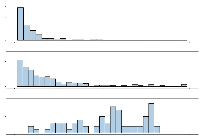
OOB Absence Proportion

Frequency

Figure 1: Histograms for each example’s distribution of OOB absence proportions.

parameters. Moreover, to account for the inherent randomness in the random forests al-

gorithm, we repeat each of our examples 1000 times with a diﬀerent random seed used to

initialize each experimental replication. However, because of the way in which we have

structured our code, we note that our analysis is able to isolate the eﬀects of the naive

and missing data heuristics on the absent levels problem since, within each experimental

replication, their underlying random forest models are identical with respect to each tree’s

in-bag training data and diﬀer only in terms of their treatment of the absent levels. As a

result, the predictions and inferences obtained from the naive and missing data heuristics

will be positively correlated across the 1000 experimental replications that we consider for

each example—a fact which we exploit in order to improve the precision of our comparisons.

Recall from Section 4, however, that the random forest models which are trained on fea-

ture engineered data sets are intrinsically diﬀerent from the random forest models which are

trained on their original untransformed data set counterparts. Therefore, although we use

the same default randomForest R package settings and the same random seed to initialize

each of the One-Hot heuristic’s experimental replications, we note that its predictions and

inferences will be essentially uncorrelated with the naive and missing data heuristics across

each example’s 1000 experimental replications.

5.1 1985 Auto Imports

For a regression example, we consider the 1985 Auto Imports data set from the UCI Machine

Learning Repository (Lichman, 2013) which, after discarding observations with missing

data, contains 25 predictors that can be used to predict the prices of 159 cars. Categorical

predictors for which the absent levels problem can occur include a car’s make (18 levels),

The “Absent Levels” Problem

Statistic 1985 Auto Imports PROMESA Pittsburgh Bridges

Min 0.003 0.001 0.080

1st Quartile 0.021 0.020 0.368

Median 0.043 0.088 0.564

Mean 0.076 0.162 0.526

3rd Quartile 0.093 0.206 0.702

Max 0.498 0.992 0.820

Table 1: Summary statistics for each example’s distribution of OOB absence proportions.

body style (5 levels), drive layout (3 levels), engine type (5 levels), and fuel system (6 levels).

Furthermore, because all of the car prices are positive, we know from Section 3.1 that the

random forests FORTRAN code and the randomForest R package will both always employ the

Left heuristic when faced with absent levels for this particular data set.

The top panel in Figure 1 depicts a histogram of this example’s OOB absence propor-

tions, which we deﬁne for each training observation as the proportion of its OOB trees

across all 1000 experimental replications which had the absent levels problem occur at least

once when using the training set with the original untransformed categorical predictors.

Meanwhile, Table 1 provides a more detailed summary of this example’s distribution of

OOB absence proportions. Consequently, although there is a noticeable right skew in the

distribution, we see that most of the observations in this example had the absent levels

problem occur in less than 5% of their OOB trees.

Let ˆy

(h)

denote the OOB prediction that a heuristic h makes for an observation n

in an experimental replication r. Then, within each experimental replication r, we can

compare the predictions that two diﬀerent heuristics h

, h

∈ H make for an observation

n by considering the diﬀerence ˆy

)

− ˆy

)

. We summarize these comparisons for all

possible pairwise combinations of the seven heuristics in Figure 2, where each panel plots

the mean and middle 95% of these diﬀerences across all 1000 experimental replications as

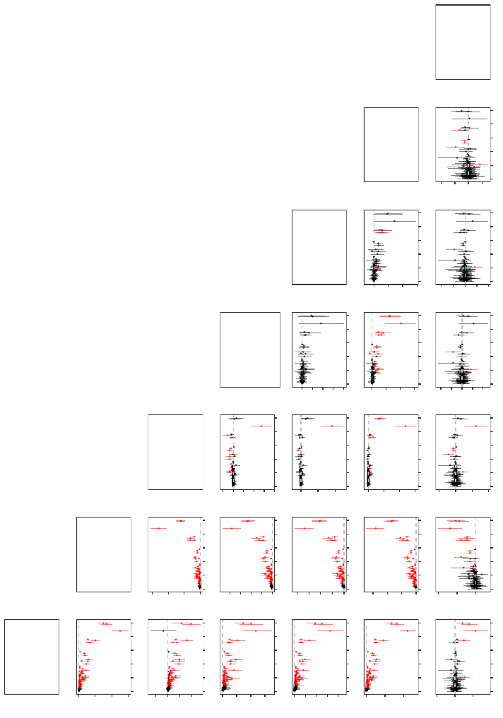
a function of the OOB absence proportion. From the red intervals in Figure 2, we see

that signiﬁcant diﬀerences in the predictions of the heuristics do exist, with the magnitude

of the point estimates and the width of the intervals tending to increase with the OOB

absence proportion—behavior that agrees with our intuition that the distinctive eﬀects of

each heuristic should become more pronounced the more often the absent levels problem

occurs.

In addition, we can evaluate the overall performance of each heuristic h ∈ H within an

experimental replication r in terms of its root mean squared error (RMSE):

RMSE

(h)

n=1



− ˆy

(h)



This is the case for versions 4.6-7 and earlier of the randomForest R package. Beginning in version 4.6-9,

however, the randomForest R package began to internally mean center the training responses prior to ﬁtting

the model, with the mean being subsequently added back to the predictions of each node. Consequently, the

Left heuristic isn’t always used in these versions of the randomForest R package since the training responses

that the model actually considers are of mixed sign. Nevertheless, such a strategy still fails to explicitly

address the underlying absent levels problem.

Left

−6000

−4000

−2000

0.0 0.1 0.2 0.3 0.4 0.5

Right

−1000

−500

500

0.0 0.1 0.2 0.3 0.4 0.5

2000

4000

6000

0.0 0.1 0.2 0.3 0.4 0.5

Stop

−1500

−1000

−500

0.0 0.1 0.2 0.3 0.4 0.5

1000

2000

3000

4000

0.0 0.1 0.2 0.3 0.4 0.5

−2000

−1500

−1000

−500

500

0.0 0.1 0.2 0.3 0.4 0.5

Majority

−2000

−1500

−1000

−500

0.0 0.1 0.2 0.3 0.4 0.5

1000

2000

3000

4000

0.0 0.1 0.2 0.3 0.4 0.5

−2000

−1000

0.0 0.1 0.2 0.3 0.4 0.5

−1000

−750

−500

−250

0.0 0.1 0.2 0.3 0.4 0.5

Random

−2000

−1000

0.0 0.1 0.2 0.3 0.4 0.5

1000

2000

3000

0.0 0.1 0.2 0.3 0.4 0.5

−3000

−2000

−1000

0.0 0.1 0.2 0.3 0.4 0.5

−1500

−1000

−500

0.0 0.1 0.2 0.3 0.4 0.5

−1200

−800

−400

0.0 0.1 0.2 0.3 0.4 0.5

DBI

−2000

2000

0.0 0.1 0.2 0.3 0.4 0.5

2000

4000

0.0 0.1 0.2 0.3 0.4 0.5

−4000

−2000

2000

0.0 0.1 0.2 0.3 0.4 0.5

−2000

−1000

1000

2000

0.0 0.1 0.2 0.3 0.4 0.5

−2000

−1000

1000

2000

0.0 0.1 0.2 0.3 0.4 0.5

−1000

1000

2000

0.0 0.1 0.2 0.3 0.4 0.5

One−Hot

OOB Absence Proportion

Difference in OOB Prediction

Figure 2: Pairwise diﬀerences in the OOB predictions as a function of the OOB absence proportions in the 1985 Auto Imports

data set. Each panel plots the mean and middle 95% of the diﬀerences across all 1000 experimental replications when the

OOB predictions of the heuristic that is labeled at the right of the panel’s row is subtracted from the OOB predictions

of the heuristic that is labeled at the top of the panel’s column. Diﬀerences were taken within each experimental

replication in order to account for the positive correlation that exists between the naive and missing data heuristics.

Intervals containing zero (the horizontal dashed line) are in black, while intervals not containing zero are in red.

The “Absent Levels” Problem

●

1900

2000

2100

2200

Left Right Stop Majority Random DBI One−Hot

RMSE

●

●●

●

−5

Left Right Stop Majority Random DBI One−Hot

Relative RMSE (%)

Absent Levels Heuristic

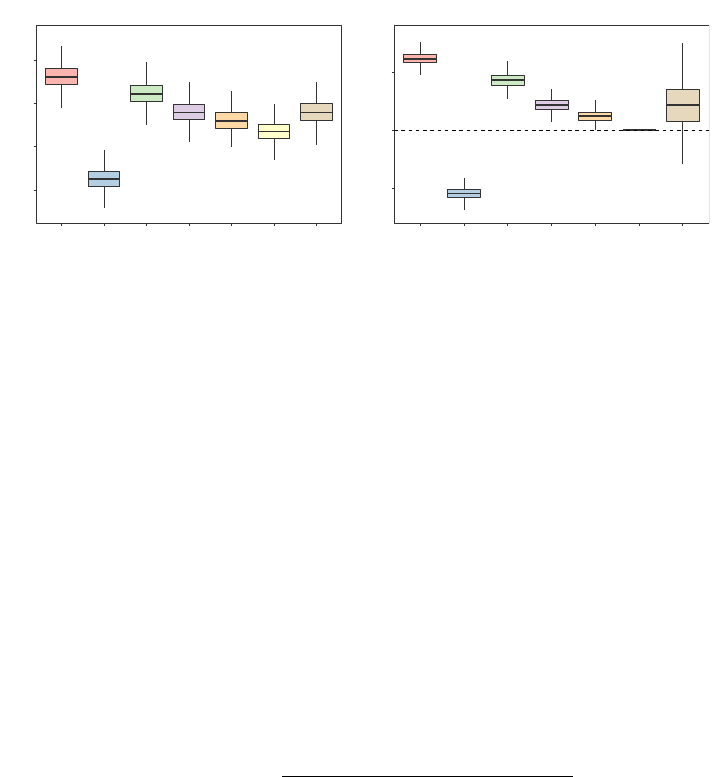
Figure 3: RMSEs for the OOB predictions of the seven heuristics in the 1985 Auto Imports

data set. The left panel shows boxplots of each heuristic’s marginal distribution of

RMSEs across all 1000 experimental replications, which ignores the positive corre-

lation that exists between the naive and missing data heuristics. The right panel

accounts for this positive correlation by comparing the RMSEs of the heuristics

relative to the best RMSE that was obtained amongst the missing data heuristics

within each of the 1000 experimental replications as in (13).

Boxplots displaying each heuristic’s marginal distribution of RMSEs across all 1000 ex-

perimental replications are shown in the left panel of Figure 3. However, these marginal

boxplots ignore the positive correlation that exists between the naive and missing data

heuristics. Therefore, within every experimental replication r, we also compare the RMSE

for each heuristic h ∈ H relative to the best RMSE that was achieved amongst the missing

data heuristics H

= {Stop, Majority, Random, DBI }:

RMSE

(hkH

)

RMSE

(h)

− min

h∈H

RMSE

(h)

min

h∈H

RMSE

(h)

. (13)

Here we note that the Left and Right heuristics were not considered in the deﬁnition of the

best RMSE achieved within each experimental replication r due to the issues discussed in

Section 3, while the One-Hot heuristic was excluded from this deﬁnition since it is essentially

uncorrelated with the other six heuristics across all 1000 experimental replications. Boxplots

of these relative RMSEs are shown in the right panel of Figure 3.

5.1.1 Naive Heuristics

Relative to all of the other heuristics and consistent with our discussions in Section 3.1, we

see from Figure 2 that the Left and Right heuristics have a tendency to severely underpredict

and overpredict, respectively. Furthermore, for this particular example, we notice from

Figure 3 that the random forests FORTRAN code and the randomForest R package’s behavior

of always sending absent levels left in this particular data set substantially underperforms

relative to the other heuristics—it gives an RMSE that is, on average, 6.2% worse than

the best performing missing data heuristic. And although the Right heuristic appears to

perform exceptionally well, we again stress the misleading nature of this performance—its

tendency to overpredict just coincidentally happens to be beneﬁcial in this speciﬁc situation.

5.1.2 Missing Data Heuristics

As can be seen from Figure 2, the predictions obtained from the four missing data heuristics

are more aligned with one another than they are with the Left, Right, and One-Hot heuris-

tics. Considerable disparities in their predictions do still exist, however, and from Figure 3

we note that amongst the four missing data heuristics, the DBI heuristic clearly performs the

best. And although the Majority heuristic fares slightly worse than the Random heuristic,

they both perform appreciably better than the Stop heuristic.

5.1.3 Feature Engineering Heuristic

Recall that the One-Hot heuristic is essentially uncorrelated with the other six heuristics

across all 1000 experimental replications—a fact which is reﬂected in its noticeably wider

intervals in Figure 2 and in its larger relative RMSE boxplot in Figure 3. Nevertheless, it

can still be observed from Figure 3 that although the One-Hot heuristic’s predictions are

sometimes able to outperform the other heuristics, on average, it yields an RMSE that is

2.2% worse than than the best performing missing data heuristic.

5.2 PROMESA

For a binary classiﬁcation example, we consider the June 9, 2016 United States House of

Representatives vote on the Puerto Rico Oversight, Management, and Economic Stability

Act (PROMESA) for addressing the Puerto Rican government’s debt crisis. Data for this

vote was obtained by using the Rvoteview R package to query the Voteview database (Lewis,

2015). After omitting those who did not vote on the bill, the data set contains four predictors

that can be used to predict the binary “No” or “Yes” votes of 424 House of Representative

members. These predictors include a categorical predictor for a representative’s political

party (2 levels), a categorical predictor for a representative’s state (50 levels), and two

ordered predictors which quantify aspects of a representative’s political ideological position

(McCarty et al., 1997).

The “No” vote was taken to be the k = 1 response class in our analysis, while the “Yes”

vote was taken to be the k = 2 response class. Recall from Section 3.2, that this ordering of

the response classes is meaningful in a binary classiﬁcation context since the randomForest

R package will always use the Left heuristic which biases predictions for observations with

absent levels towards whichever response class is indexed by k = 2 (corresponding to the

“Yes” vote in our analysis).

From Figure 1 and Table 1, we see that the absent levels problem occurs much more

frequently in this example than it did in our 1985 Auto Imports example. In particular, the

seven House of Representative members who were the sole representatives from their state

had OOB absence proportions that were greater than 0.961 since the absent levels problem

occurred for these observations every time they reached an OOB tree node that was split

on the state predictor.

For random forest classiﬁcation models, the predicted probability that an observation

belongs to a response class k can be estimated by the proportion of the observation’s trees

The “Absent Levels” Problem

Left

0.00

0.25

0.50

0.75

1.00

0.00 0.25 0.50 0.75 1.00

Right

−0.1

0.0

0.1

0.2

0.3

0.4

0.00 0.25 0.50 0.75 1.00

−0.75

−0.50

−0.25

0.00

0.00 0.25 0.50 0.75 1.00

Stop

0.0

0.2

0.4

0.6

0.00 0.25 0.50 0.75 1.00

−0.6

−0.4

−0.2

0.0

0.00 0.25 0.50 0.75 1.00

0.0

0.2

0.4

0.00 0.25 0.50 0.75 1.00

Majority

0.0

0.2

0.4

0.00 0.25 0.50 0.75 1.00

−0.6

−0.4

−0.2

0.0

0.00 0.25 0.50 0.75 1.00

0.0

0.2

0.4

0.00 0.25 0.50 0.75 1.00

−0.1

0.0

0.1

0.00 0.25 0.50 0.75 1.00

Random

0.0

0.2

0.4

0.00 0.25 0.50 0.75 1.00

−0.8

−0.6

−0.4

−0.2

0.0

0.00 0.25 0.50 0.75 1.00

−0.1

0.0

0.1

0.2

0.3

0.00 0.25 0.50 0.75 1.00

−0.2

−0.1

0.0

0.00 0.25 0.50 0.75 1.00

−0.2

−0.1

0.0

0.1

0.00 0.25 0.50 0.75 1.00

DBI

−0.50

−0.25

0.00

0.25

0.50

0.00 0.25 0.50 0.75 1.00

−0.75

−0.50

−0.25

0.00

0.25

0.00 0.25 0.50 0.75 1.00

−0.50

−0.25

0.00

0.25

0.00 0.25 0.50 0.75 1.00

−0.50

−0.25

0.00

0.25

0.00 0.25 0.50 0.75 1.00

−0.4

−0.2

0.0

0.2

0.00 0.25 0.50 0.75 1.00

−0.50

−0.25

0.00

0.25

0.00 0.25 0.50 0.75 1.00

One−Hot

OOB Absence Proportion

Difference in OOB Prediction

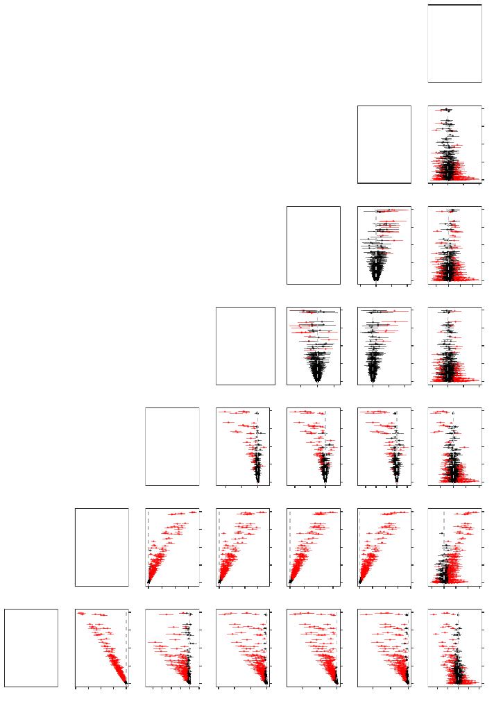
Figure 4: Pairwise diﬀerences in the OOB predicted probabilities of voting “Yes” as a function of the OOB absence proportion

in the PROMESA data set. Each panel plots the mean and middle 95% of the pairwise diﬀerences across all 1000

experimental replications when the OOB predicted probabilities of the heuristic that is labeled at the right of the

panel’s row is subtracted from the OOB predicted probabilities of the heuristic that is labeled at the top of the panel’s

column. Diﬀerences were taken within each experimental replication to account for the positive correlation that exists

between the naive and missing data heuristics. Intervals containing zero (the horizontal dashed line) are in black, while

intervals not containing zero are in red.

which classify it to class k.

Let ˆp

(h)

nkr

denote the OOB predicted probability that a heuristic

h assigns to an observation n of belonging to a response class k in an experimental replication

r. Then, within each experimental replication r, we can compare the predicted probabilities

that two diﬀerent heuristics h

, h

∈ H assign to an observation n by considering the

diﬀerence ˆp

)

nkr

− ˆp

)

nkr

. We summarize these diﬀerences in the predicted probabilities of

voting “Yes” for all possible pairwise combinations of the seven heuristics in Figure 4, where

each panel plots the mean and middle 95% of these diﬀerences across all 1000 experimental

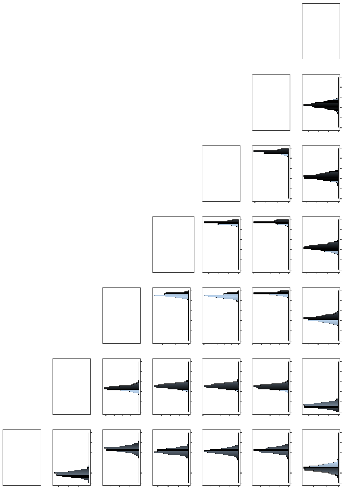
replications as a function of the OOB absence proportion.

The large discrepancies in the predicted probabilities that are observed in Figure 4 are

particularly concerning since they can lead to diﬀerent classiﬁcations. If we let ˆy

(h)

denote

the OOB classiﬁcation that a heuristic h makes for an observation n in an experimental

replication r, then Cohen’s kappa coeﬃcient (Cohen, 1960) provides one way of measuring

the level of agreement between two diﬀerent heuristics h

, h

∈ H:

)

− e

)

1 − e

)

, (14)

where

)

n=1



ˆy

)

= ˆy

)



is the observed probability of agreement between the two heuristics, and where

)

k=1

n=1



ˆy

)

= k



n=1



ˆy

)

= k



is the expected probability of the two heuristics agreeing by chance. Therefore, within an

experimental replication r, we will observe κ

)

= 1 if the two heuristics are in com-

plete agreement, and we will observe κ

)

≈ 0 if there is no agreement amongst the two

heuristics other than what would be expected by chance. In Figure 5, we plot histograms

of the Cohen’s kappa coeﬃcient for all possible pairwise combinations of the seven heuris-

tics across all 1000 experimental replications when the random forests algorithm’s default

majority vote discrimination threshold of 0.5 is used.

More generally, the areas underneath the receiver operating characteristic (ROC) and

precision-recall (PR) curves can be used to compare the overall performance of binary

classiﬁers as the discrimination threshold is varied between 0 and 1. Speciﬁcally, as the dis-

crimination threshold changes, the ROC curve plots the proportion of positive observations

that a classiﬁer correctly labels as a function of the proportion of negative observations

that a classiﬁer incorrectly labels, while the PR curve plots the proportion of a classiﬁer’s

positive labels that are truly positive as a function of the proportion of positive observations

that a classiﬁer correctly labels (Davis and Goadrich, 2006).

This is the approach that is used by the randomForest R package. The scikit-learn Python module

uses an alternative method of calculating the predicted response class probabilities which takes the average

of the predicted class probabilities over the trees in the random forest, where the predicted probability of

a response class k in an individual tree is estimated using the proportion of a node’s training samples that

belong to the response class k.

The “Absent Levels” Problem

Left

100

150

0.5 0.6 0.7 0.8 0.9 1.0

Right

100

150

0.5 0.6 0.7 0.8 0.9 1.0

100

150

200

0.5 0.6 0.7 0.8 0.9 1.0

Stop

100

150

0.5 0.6 0.7 0.8 0.9 1.0

100

150

0.5 0.6 0.7 0.8 0.9 1.0

100

200

0.5 0.6 0.7 0.8 0.9 1.0

Majority

100

150

0.5 0.6 0.7 0.8 0.9 1.0

100

150

200

0.5 0.6 0.7 0.8 0.9 1.0

100

150

200

250

0.5 0.6 0.7 0.8 0.9 1.0

100

200

300

0.5 0.6 0.7 0.8 0.9 1.0

Random

100

150

0.5 0.6 0.7 0.8 0.9 1.0

100

150

0.5 0.6 0.7 0.8 0.9 1.0

100

200

300

400

0.5 0.6 0.7 0.8 0.9 1.0

100

200

300

400

0.5 0.6 0.7 0.8 0.9 1.0

100

200

300

0.5 0.6 0.7 0.8 0.9 1.0

DBI

100

0.5 0.6 0.7 0.8 0.9 1.0

100

150

0.5 0.6 0.7 0.8 0.9 1.0

100

150

0.5 0.6 0.7 0.8 0.9 1.0

100

150

0.5 0.6 0.7 0.8 0.9 1.0

100

150

0.5 0.6 0.7 0.8 0.9 1.0

100

150

0.5 0.6 0.7 0.8 0.9 1.0

One−Hot

Cohen's Kappa

Frequency

Figure 5: Pairwise Cohen’s kappa coeﬃcients for the seven diﬀerent heuristics as deﬁned in (14) when the random forests algo-

rithm’s default majority vote discrimination threshold of 0.5 is used in the PROMESA data set. Each panel plots the

histogram of coeﬃcients across all 1000 experimental replications when the OOB classiﬁcations of the heuristic that

is labeled at the right of the panel’s row are compared against the OOB classiﬁcations of the heuristic that is labeled

at the top of the panel’s column. Cohen’s kappa coeﬃcients were calculated within each of the 1000 experimental

replications to account for the positive correlation between the naive and missing data heuristics.

Taking the “Yes” vote to be the positive response class in our analysis, we calculate the

areas underneath the ROC and PR curves for each heuristic h ∈ H within each experimental

replication r. Boxplots depicting each heuristic’s marginal distribution of these two areas

across all 1000 experimental replications are shown in the left panels of Figure 6. However,

these marginal boxplots ignore the positive correlation that exists between the naive and

missing data heuristics. Therefore, within every experimental replication r and similar to

what was previously done in our 1985 Auto Imports example, we also compare the areas

for each heuristic h ∈ H relative to the best area that was achieved amongst the missing

data heuristics H

= {Stop, Majority, Random, DBI }:

AUC

(hkH

)

AUC

(h)

− max

h∈H

AUC

(h)

max

h∈H

AUC

(h)

, (15)

where, depending on the context, AUC

(h)

denotes the area that is underneath either the

ROC or PR curve for heuristic h in experimental replication r. Boxplots of these relative

areas across all 1000 experimental replications are displayed in the right panels of Figure 6.

5.2.1 Naive Heuristics

As expected given our discussions in Section 3.2 and how we have chosen to index the

response classes in our analysis, we see from Figure 4 that the Left heuristic results in sig-

niﬁcantly higher predicted probabilities of voting “Yes” than the other heuristics, while the

Right heuristic yields predicted probabilities of voting “Yes” that are substantially lower.

The consequences of this behavior in terms of making classiﬁcations can be observed in

Figure 5, where we note that both the Left and Right heuristics tend to exhibit a high level

of disagreement when compared against any other heuristic’s classiﬁcations. Moreover, Fig-

ure 6 illustrates that the randomForest R package’s practice of always sending absent levels

left in binary classiﬁcation is noticeably detrimental here—relative to the best performing

missing data heuristic, it gives areas underneath the ROC and PR curves that are, on av-

erage, 1.5% and 3.7% worse, respectively. And although the Right heuristic appears to do

well in terms of the area underneath the PR curve, we once again emphasize the spurious

nature of this performance and caution against taking it at face value.

5.2.2 Missing Data Heuristics

Similar to what was previously seen in our 1985 Auto Imports example, Figures 4 and 5

show that the four missing data heuristics tend to exhibit a higher level of agreement with

one another than they do with the Left, Right, and One-Hot heuristics. However, signiﬁcant

diﬀerences do still exist, and we see from Figure 6 that the relative performances of the

heuristics will vary depending on the speciﬁc task at hand—the Majority heuristic slightly

outperforms the three other missing data heuristics in terms of the area underneath the

ROC curve, while the Random heuristic does considerably better than all of its missing

data counterparts with respect to the area underneath the PR curve.

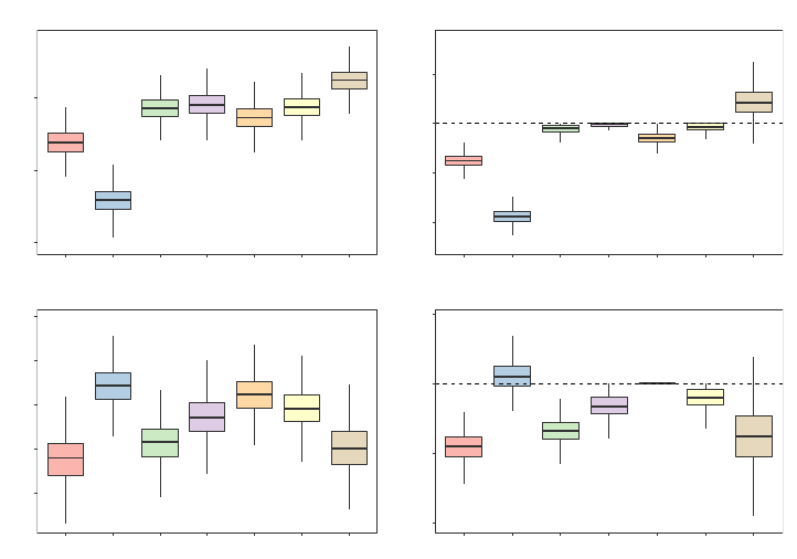
The “Absent Levels” Problem

●

0.68

0.70

0.72

Left Right Stop Majority Random DBI One−Hot

Receiver Operating Characteristic (ROC) Curve

●

0.76

0.78

0.80

0.82

0.84

Left Right Stop Majority Random DBI One−Hot

Precision−Recall (PR) Curve

Area

●

−4

−2

Left Right Stop Majority Random DBI One−Hot

Receiver Operating Characteristic (ROC) Curve

●

−8

−4

Left Right Stop Majority Random DBI One−Hot

Precision−Recall (PR) Curve

Relative Area (%)

Absent Levels Heuristic

Figure 6: Areas underneath the ROC and PR curves for the seven heuristics in the

PROMESA data set. The left panels show boxplots of each heuristic’s marginal

distribution of areas across all 1000 experimental replications, which ignores the

positive correlation that exists between the naive and missing data heuristics.

The right panels account for this positive correlation by comparing the areas of

the heuristics relative to the best area that was obtained amongst the missing

data heuristics within each of the 1000 experimental replications as in (15).

5.2.3 Feature Engineering Heuristic

Although it is essentially uncorrelated with the other six heuristics across all 1000 exper-

imental replications, Figures 4 and 5 still suggest that the One-Hot heuristic’s predicted

probabilities and classiﬁcations can greatly diﬀer from the other six heuristics. Further-

more, Figure 6 shows that even though the One-Hot heuristic may appear to perform well

in terms of the area underneath its ROC curve relative to the missing data heuristics, its

performance in the PR context is rather lackluster.

5.3 Pittsburgh Bridges

For a multiclass classiﬁcation example, we consider the Pittsburgh Bridges data set from

the UCI Machine Learning Repository which, after removing observations with missing

data, contains seven predictors that can be used to classify 72 bridges to one of seven

diﬀerent bridge types. The categorical predictors in this data set for which the absent levels

problem can occur include a bridge’s river (3 levels), purpose (3 levels), and location (46

levels). Consequently, recall from Section 3.2, that the random forests FORTRAN code and

randomForest R package will both employ an exhaustive search that always sends absent

levels right when splitting on either the river or purpose predictors, and that they will

both resort to using a random search that sends absent levels either left or right with equal

probability when splitting on the location predictor since it has too many levels for an

exhaustive search to be computationally eﬃcient. The OOB absence proportions for this

example are summarized in the bottom panel of Figure 1 and in Table 1.

Within each experimental replication r, we can use the log loss

LogLoss

(h)

= −

n=1

k=1

I(y

= k) · log



ˆp

(h)

nkr

i

to evaluate the overall performance of each heuristic h ∈ H, where we once again let

ˆp

(h)

nkr

denote the OOB predicted probability that a heuristic h assigns to an observation

n of belonging to a response class k in an experimental replication r. The left panel of

Figure 7 displays the marginal distribution of each heuristic’s log losses across all 1000

experimental replications. However, to once again account for the positive correlation that

exists amongst the naive and missing data heuristics, within every experimental replication

r, we also compare the log losses for each heuristic h ∈ H relative to the best log loss that

was achieved amongst the missing data heuristics H

= {Stop, Majority, Random, DBI }:

LogLoss

(hkH

)

LogLoss

(h)

− min

h∈H

LogLoss

(h)

min

h∈H

LogLoss

(h)

. (16)

Boxplots of these relative log losses are depicted in the right panel of Figure 7.

5.3.1 Naive Heuristics

Although we once again stress the systematically biased nature of the Left and Right heuris-

tics, we note from Figure 7 that the two naive heuristics are sometimes able to outperform

the missing data heuristics. Nevertheless, on average, the Left and Right heuristics resulted

in log losses that are 0.7% and 1.9% worse than the best performing missing data heuristic,

respectively.

5.3.2 Missing Data Heuristics

Figure 7 shows that for this particular example, the Majority and Random heuristics per-

form roughly on par with one another, and that they both also signiﬁcantly outperform

the Stop and DBI heuristics—the smallest log loss amongst all of the missing data heuris-

tics was achieved by either the Majority or the Random heuristic in 999 out of the 1000

experimental replications.

5.3.3 Feature Engineering Heuristic

It can also be observed from Figure 7 that, although the One-Hot heuristic can occasionally

outperform the missing data heuristics, on average, it yields a log loss that is 4.5% worse

than the best performing missing data heuristic.

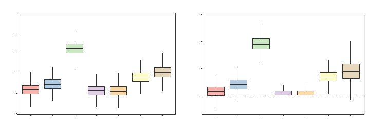
The “Absent Levels” Problem

●

1.10

1.15

1.20

1.25

1.30

Left Right Stop Majority Random DBI OneHot

Log Loss

●

●●

●

Left Right Stop Majority Random DBI OneHot

Relative Log Loss (%)

Absent Levels Heuristic

Figure 7: Log losses for the OOB predicted response class probabilities of the seven heuris-

tics in the Pittsburgh Bridges data. The left panel shows boxplots of each heuris-

tic’s marginal distribution of log losses set across all 1000 experimental replica-

tions, which ignores the positive correlation that exists between the naive and

missing data heuristics. The right panel accounts for this positive correlation by

comparing the log losses of the heuristics relative to the best log loss that was ob-

tained amongst the missing data heuristics within each of the 1000 experimental

replications as in (16).

6. Conclusion

In this paper, we introduced and investigated the absent levels problem for decision tree

based methods. In particular, by using Breiman and Cutler’s random forests FORTRAN code

and the randomForest R package as motivating case studies, we showed how overlooking the

absent levels problem could systematically bias a model. Furthermore, we presented three

real data examples which illustrated how absent levels can dramatically alter a model’s

performance in practice.

Even though a comprehensive theoretical analysis of the absent levels problem was

beyond the scope of this paper, we empirically demonstrated how some simple heuristics

could be used to help mitigate the eﬀects of absent levels. And although none of the missing

data and feature engineering heuristics that we considered performed uniformly better than

all of the others, they were all shown to be superior to the biased naive approaches that

are currently being employed due to oversights in the software implementations of decision

tree based methods.

Consequently, until a more robust theoretical solution is found, we encourage the soft-

ware implementations which support the native categorical split capabilities of decision trees

to incorporate the Random heuristic as a provisional measure given its reliability—in all of

our examples, the Random heuristic was always competitive in terms of its performance.

Moreover, based on our own personal experiences, we note that the Random heuristic was

one of the easier heuristics to implement on top of the randomForest R package. In the

meantime, while waiting for these mitigations to materialize, we also urge users who rely

on decision tree based methods to feature engineer their data sets when possible in order to

circumvent the absent levels problem—although our empirical results suggest that this may

sometimes be detrimental to a model’s performance, we believe this to still be preferable

to the alternative of having to rely on biased approaches which do not adequately address

absent levels.

Finally, although this paper primarily focused on the absent levels problem for random

forests and a particular subset of the types of analyses in which random forests have been

used, it is important to recognize that the issue of absent levels applies much more broadly.

For example, decision tree based methods have also been employed for clustering, detecting

outliers, imputing missing values, and generating variable importance measures (Breiman,

2003)—tasks which also depend on the terminal node behavior of the observations. In ad-

dition, several extensions of decision tree based methods have been built on top of software

which currently overlook absent levels—such as the quantile regression forests algorithm

(Meinshausen, 2006, 2012) and the inﬁnitesimal jackknife method for estimating the vari-

ance of bagged predictors (Wager et al., 2014), which are both implemented on top of the

randomForest R package. Indeed, given how extensively decision tree based methods have

been used, a sizable number of these models have almost surely been signiﬁcantly and un-

knowingly aﬀected by the absent levels problem in practice—further emphasizing the need

for the development of both theory and software that accounts for this issue.

Acknowledgements

The author is extremely grateful to Art Owen for numerous valuable discussions and in-

sightful comments which substantially improved this paper. The author would also like to

thank David Chan, Robert Bell, the action editor, and the anonymous reviewers for their

helpful feedback. Finally, the author would like to thank Jim Koehler, Tim Hesterberg,

Joseph Kelly, Iv´an D´ıaz, Jingang Miao, and Aiyou Chen for many interesting discussions.

References

Yali Amit and Donald Geman. Shape quantization and recognition with randomized trees.

Neural Computation, 9:1545–1588, 1997.

G´erard Biau. Analysis of a random forests model. Journal of Machine Learning Research,

13(1):1063–1095, 2012.

G´erard Biau, Luc Devroye, and G´abor Lugosi. Consistency of random forests and other

averaging classiﬁers. Journal of Machine Learning Research, 9(1):2015–2033, 2008.

Leo Breiman. Bagging predictors. Machine Learning, 24(2):123–140, 1996a.

Leo Breiman. Out-of-bag estimation. Technical report, Department of Statistics, U.C.

Berkeley, 1996b. URL https://www.stat.berkeley.edu/

breiman/OOBestimation.

pdf.

Leo Breiman. Random forests. Machine Learning, 45(1):5–32, 2001.

Leo Breiman. Manual—setting up, using, and understanding random forest v4.0. 2003.

URL https://www.stat.berkeley.edu/

breiman/Using_random_forests_v4.0.pdf.

The “Absent Levels” Problem

Leo Breiman, Jerome. H. Friedman, Richard. A. Olshen, and Charles J. Stone. Classiﬁcation

and Regression Trees. Wadsworth, 1984. ISBN 0-534-98053-8.

Jacob Cohen. A coeﬃcient of agreement for nominal scales. Educational and Psychological

Measurement, 20:37–46, 1960.

Jesse Davis and Mark Goadrich. The relationship between precision-recall and ROC curves.

In ICML ’06: Proceedings of the 23rd international conference on Machine learning, pages

233–240, 2006.

Misha Denil, David Matheson, and Nando de Freitas. Narrowing the gap: Random forests

in theory and in practice. In Proceedings of the 31th International Conference on Machine

Learning, pages 665–673, 2014.

Walter D. Fisher. On grouping for maximum homogeneity. Journal of the American Sta-

tistical Association, 53(284):789–798, 1958.

Trevor J Hastie, Robert J. Tibshirani, and Jerome H. Friedman. The Elements of Statistical

Learning: Data Mining, Inference, and Prediction, Second Edition. Springer Series in

Statistics. Springer, New York, 2009.

Tin Kam Ho. The random subspace method for constructing decision forests. IEEE Trans-

actions on Pattern Analysis and Machine Intelligence, 20(8):832–844, 1998.

Torsten Hothorn and Achim Zeileis. partykit: A modular toolkit for recursive partytioning

in R. Journal of Machine Learning Research, 16:3905–3909, 2015.

Torsten Hothorn, Kurt Hornik, and Achim Zeileis. Unbiased recursive partitioning: A

conditional inference framework. Journal of Computational and Graphical Statistics, 15

(3):651–674, 2006.

Hemant Ishwaran, Udaya B. Kogalur, Eugene H. Blackstone, and Michael S. Lauer. Random

survival forests. Annals of Applied Statistics, 2(3):841–860, 2008.

Jeﬀ Lewis. Rvoteview: Voteview Data in R, 2015. https://github.com/JeffreyBLewis/

Rvoteview, http://voteview.polisci.ucla.edu, http://voteview.com.

Andy Liaw and Matthew Wiener. Classiﬁcation and regression by randomForest. R News,

2(3):18–22, 2002.

Moshe Lichman. UCI machine learning repository, 2013. URL http://archive.ics.uci.

edu/ml.

Wei-Yin Loh and Nunta Vanichsetakul. Tree-structured classiﬁcation via generalized dis-

criminant analysis. Journal of the American Statistical Association, 83(403):715–725,

1988.

Nolan M. McCarty, Keith T. Poole, and Howard Rosenthal. Income Redistribution and

the Realignment of American Politics. AEI Press, publisher for the American Enterprise

Institute, 1997.

Nicolai Meinshausen. Quantile regression forests. Journal of Machine Learning Research,

7:983–999, 2006.

Nicolai Meinshausen. quantregForest: Quantile Regression Forests, 2012. URL http://

CRAN.R-project.org/package=quantregForest. R package version 0.2-3.

Fabian Pedregosa, Ga¨el Varoquaux, Alexandre Gramfort, Vincent Michel, Bertrand

Thirion, Olivier Grisel, Mathieu Blondel, Peter Prettenhofer, Ron Weiss, Vincent

Dubourg, Jake Vanderplas, Alexandre Passos, David Cournapeau, Matthieu Brucher,

Matthieu Perrot, and

Edouard Duchesnay. Scikit-learn: Machine learning in Python.

Journal of Machine Learning Research, 12:2825–2830, 2011.

John R. Quinlan. C4.5: Programs for Machine Learning. Morgan Kaufmann Publishers

Inc., 1993.

Greg Ridgeway. gbm: Generalized Boosted Regression Models, 2013. URL http://CRAN.

R-project.org/package=gbm. R package version 2.1.

Brian D. Ripley. Pattern Recognition and Neural Networks. Cambridge University Press,

Cambridge, 1996. ISBN 0-521-46086-7.

Maytal Saar-Tsechansky and Foster Provost. Handling missing values when applying clas-

siﬁcation models. Journal of Machine Learning Research, 8:1623–1657, 2007.

Terry Therneau, Beth Atkinson, and Brian Ripley. rpart: Recursive Partitioning and Re-

gression Trees, 2015. URL http://CRAN.R-project.org/package=rpart. R package

version 4.1-10.

Stefan Wager, Trevor Hastie, and Bradley Efron. Conﬁdence intervals for random forests:

The jackknife and the inﬁnitesimal jackknife. Journal of Machine Learning Research, 15

(1):1625–1651, 2014.