Privately Evaluating Decision Trees and Random Forests

(Extended Version)

David J. Wu

∗

Tony Feng

∗

Michael Naehrig

†

Kristin Lauter

†

Abstract

Decision trees and random forests are common classiﬁers with widespread use. In this paper,

we develop two protocols for privately evaluating decision trees and random forests. We operate

in the standard two-party setting where the server holds a model (either a tree or a forest),

and the client holds an input (a feature vector). At the conclusion of the protocol, the client

learns only the model’s output on its input and a few generic parameters concerning the model;

the server learns nothing. The ﬁrst protocol we develop provides security against semi-honest

adversaries. We then give an extension of the semi-honest protocol that is robust against

malicious adversaries. We implement both protocols and show that both variants are able to

process trees with several hundred decision nodes in just a few seconds and a modest amount

of bandwidth. Compared to previous semi-honest protocols for private decision tree evaluation,

we demonstrate a tenfold improvement in computation and bandwidth.

1 Introduction

In recent years, machine learning has been successfully applied to many areas, such as spam clas-

siﬁcation, credit-risk assessment, cancer diagnosis, and more. With the transition towards cloud-

based computing, this has enabled many useful services for consumers. For example, there are

many companies that provide automatic medical assessments and risk proﬁles for various diseases

by evaluating a user’s responses to an online questionnaire, or by analyzing a user’s DNA proﬁle.

In the personal ﬁnance area, there exist automatic tools and services that provide valuations for a

user’s car or property based on information the user provides. In most cases, these services require

access to the user’s information in the clear. Many of these situations involve potentially sensitive

information, such as a user’s medical or ﬁnancial data. A natural question to ask is whether one

can take advantage of cloud-based machine learning, and still maintain the privacy of the user’s

data. On the ﬂip side, in many situations, we also require privacy for the model. For example,

in scenarios where companies leverage learned models for providing product recommendations, the

details of the underlying model often constitute an integral part of the company’s “secret sauce,”

and thus, eﬀorts are taken to guard the precise details. In other scenarios, the model might have

been trained on sensitive information such as the results from a medical study or patient records

from a hospital; here, revealing the model can compromise sensitive information as well as violate

certain laws and regulations.

∗

Stanford University - [email protected], [email protected]. Work done while at Microsoft Research.

†

Microsoft Research - {mnaehrig, klauter}@microsoft.com.

In this work, we focus on one commonly used class of classiﬁers: decision trees and random

forests [43, 19]. Decision trees are simple classiﬁers that consist of a collection of decision nodes

arranged in a tree structure. As the name suggests, each decision node is associated with a pred-

icate or test on the query (for example, a possible predicate could be “age > 55”). Decision tree

evaluation simply corresponds to tree traversal. These models are often favored by users for their

ease of interpretability. In fact, there are numerous web APIs [2, 1] that enable users to both train

and query decision trees as part of a machine learning as a service platform. In spite of their simple

structure, decision trees are widely used in machine learning, and have been successfully applied to

many scenarios such as disease diagnosis [62, 5] and credit-risk assessment [49].

In this work, we develop practical protocols for private evaluation of decision trees and random

forests. In our setting, the server has a decision tree (or random forest) model and the client holds

an input to the model. Abstractly, our desired security property is that at the end of the protocol

execution, the server should not learn anything about the client’s input, and the client should not

learn anything about the server’s model other than what can be directly inferred from the output

of the model. This is a natural setting in cases where we are working with potentially sensitive

and private information on the client’s side and where we desire to protect the server’s model,

which might contain proprietary or conﬁdential information. To motivate the need for privacy, we

highlight one such application of using decision trees for automatic medical diagnosis.

Application to medical diagnosis. Decision trees are used by physicians for both automatic

medical diagnosis and medical decision making [62, 5]. A possible deployment scenario is for a

hospital consortium or a government agency to provide automatic medical diagnosis services for

other physicians to use. To leverage such a service, a physician (or even a patient) would take a

set of measurements (as speciﬁed by the model) and submit those to the service for classiﬁcation.

Of course, to avoid compromising the patient’s privacy, we require that at the end of the protocol,

the service does not learn anything about the client’s input. On the ﬂip side, there is also a need

to protect the server’s model from the physician (or patient) that is querying the service. In recent

work, Fredrikson et al. [34] showed that white-box access to a decision tree model can be eﬃciently

exploited to compromise the privacy of the users whose data was used to train the decision tree.

In this case, this means that the medical details of the patients whose medical proﬁles were used

to develop the model are potentially compromised by revealing the model in the clear. Not only

is this a serious privacy concern, in the case of medical records, this can be a violation of HIPAA

regulations. Thus, in this scenario, it is critical to provide privacy for both the input to the

classiﬁer, as well as the internal details of the classiﬁer itself. We note that even though black-box

access to a model can still be problematic, combining our private model evaluation protocol with

“privacy-aware” decision tree training algorithms [34, §6] can signiﬁcantly mitigate this risk.

1.1 Our Contributions

We begin by constructing a decision tree evaluation protocol with security against semi-honest

adversaries (i.e., adversaries that behave according to the protocol speciﬁcation). We then show how

to extend the semi-honest protocol to provide robustness against malicious adversaries. Speciﬁcally,

we show that a malicious client cannot learn additional information about the server’s model, and

that a malicious server cannot learn anything about the client’s input. Note that it is possible

for a malicious server to cause the client to obtain a corrupted or wrong output; however, even

in this case, it does not learn anything about the client’s input. This model is well-suited for

cloud-based applications where we assume the server is trying to provide a useful service, and thus,

not incentivized to give corrupt or nonsensical output to the client. In fact, because the server has

absolute control over the model in the private decision tree evaluation setting, privacy of the client’s

input is the strongest property we can hope for in the presence of a malicious server. We describe our

threat model formally in Section 2.3. Our protocols leverage two standard cryptographic primitives:

additive homomorphic encryption and oblivious transfer.

As part of our construction for malicious security, we show how a standard comparison protocol

based on additively homomorphic encryption [28] can be used to obtain an eﬃcient conditional

oblivious transfer protocol [11, 27] for the less-than predicate.

To assess the practicality of our protocols, we implement both the semi-honest protocol as well

as the extended protocol with protection against malicious adversaries using standard libraries. We

conduct experiments with decision trees with depth up to 20, as well as decision trees with over

10,000 decision nodes to assess the scalability of our protocols. We also compare the performance

of our semi-honest secure protocol against the protocols of [17, 7, 20], and demonstrate over 10x

reduction in client computation and bandwidth, or both, while operating at a higher security level

(128 bits of security as opposed to 80 bits of security in past works). We conclude our experimental

analysis by evaluating our protocols on decision trees trained on several real datasets from the

UCI repository [6]. In most cases, our semi-honest decision tree protocol completes on the order

of seconds and requires bandwidth ranging from under 100 KB to several MB. This represents

reasonable performance for a cloud-based service.

This work provides the ﬁrst implementation of a private decision tree evaluation protocol with

security against malicious adversaries. In our benchmarks, we additionally show that even with

the extensions for malicious security, our protocol still outperforms existing protocols that achieve

only semi-honest security.

Related work. This problem of privately evaluating decision trees falls under the general um-

brella of multiparty computation. One approach is based on homomorphic encryption [35, 59],

where the client sends the server an encryption of its input, and the server evaluates the function

homomorphically and sends the encrypted response back to the client. The client decrypts to learn

the output. While these methods have been successfully applied to several problems in privacy-

preserving data mining [39, 16], the methods are limited to simple functionalities. Another general

approach is based on Yao’s garbled circuits [63, 53, 51, 10, 9], where one party prepares a garbled

circuit representing the joint function they want to compute and the other party evaluates the cir-

cuit. These methods typically have large communication costs; we provide some concrete estimates

based on state-of-the-art tools in Section 6. We survey additional related work in Section 7.

2 Preliminaries

We begin with some notation. Let [n] be the set of integers {1, . . . , n}, and Z

be the ring of

integers modulo p. For two k-bit strings x, y ∈ {0, 1}

, we write x ⊕ y for their bitwise xor. For a

distribution D, we write x ← D to denote a sample s from D. For a ﬁnite set S, we write x

←− S

to denote a uniform draw x from S. We say that two distributions D

and D

are computationally

indistinguishable (denoted D

≈ D

) if no eﬃcient (that is, probabilistic polynomial time) algorithm

can distinguish them except with negligible probability. We write D

≈ D

to denote that the two

distributions D

and D

are statistically close. A function f(λ) is negligible in a parameter λ if for

all positive integers c, f = o(1/λ

). For a predicate P we write 1 {P(x)} to denote the indicator

function for the predicate P—that is, 1 {P(x)} = 1 if and only if P(x) holds, and 0 otherwise.

2.1 Cryptographic Primitives

In this section, we introduce the primitives we require.

Homomorphic encryption. A semantically secure public-key encryption system with message

space R (we model R as a ring) is speciﬁed by three algorithms KeyGen, Enc

, Dec

(for key

generation, encryption, decryption, respectively). The key-generation algorithm outputs a public-

private key pair (pk, sk). For a message m, we write Enc

(m; r) to denote an encryption of m

with randomness r. The security requirement is the standard notion of semantic security [37].

In an additively homomorphic encryption [59, 28, 29] system, we require an additional public-key

operation that takes encryptions of two messages m

, m

and outputs an encryption of m

+ m

Additionally, we require that the scheme supports scalar multiplication: given an encryption of

m ∈ R, there is a public-key operation that produces an encryption of km for all k ∈ Z.

Oblivious Transfer. Oblivious transfer (OT) [60, 56, 57, 4] is a primitive commonly employed

in cryptographic protocols. In standard 1-out-of-n OT, there are two parties, denoted the sender

and the receiver. The sender holds a database x

, . . . , x

∈ {0, 1}

and the client holds a selection

bit i ∈ [n]. At the end of the protocol, the client learns x

and nothing else about the contents of

the database; the server learns nothing.

2.2 Decision Trees and Random Forests

Decision trees are frequently encountered in machine learning and can be used for classiﬁcation

and regression. A decision tree T : Z

→ Z implements a function on an n-dimensional feature

space (the feature space is typically R

, so we use a ﬁxed-point encoding of the values). We refer to

elements x ∈ Z

as feature vectors. Each internal node v

in the tree is associated with a Boolean

function f

(x) = 1 {x

< t

}, where i

∈ [n] is an index into a feature vector x ∈ Z

, and t

a threshold. Each leaf node ` is associated with an output value z

. To evaluate the decision tree

on an input x ∈ Z

, we start at the root node, and at each internal node v

, we evaluate f

(x).

Depending on whether f

(x) evaluates to 0 or 1, we take either the left or right branch of the tree.

We repeat this process until we reach a leaf node `. The output T (x) is the value z

of the leaf

node.

The depth of a decision tree is the length of the longest path from the root to a leaf. The i

layer of the tree is the set of nodes of distance exactly i from the root. A binary tree with depth d

is complete if for 0 ≤ i ≤ d, the i

layer contains exactly 2

nodes.

Complete binary trees. In general, decision trees need not be binary or complete. However,

all decision trees can be transformed into a complete binary decision tree by increasing the depth

of the tree and introducing “dummy” internal nodes. In particular, all leaves in the subtree of a

dummy internal node have the same value. We associate each dummy node with the trivial Boolean

function f(x) = 0. Without loss of generality, we only consider complete binary decision trees in

this work.

Node indices. We use the following indexing scheme to refer to nodes in a complete binary

tree. Let T be a decision tree with depth d. Set v

to be the root node. We label the remaining

nodes inductively: if v

is an internal node, let v

be its left child and v

2i+1

be its right child. For

convenience, we also deﬁne a separate index from 0 to 2

− 1 for the leaf nodes. Speciﬁcally, if v

the parent of a leaf node, then we denote its left and right children by z

2i−m−1

and z

2i−m

, where

m is the number of internal nodes in T . With this indexing scheme, the leaves of the tree, when

read from left-to-right, correspond with the ordering z

, . . . , z

−1

Paths in a binary tree. We associate paths in a complete binary tree with bit strings. Speciﬁ-

cally, let T be a complete binary tree with depth d. We specify a path by a bit string b = b

· · · b

∈

{0, 1}

, where b

denotes whether we visit the left child or the right child when we are at a node at

level i − 1. Starting at the root node (level 0), and traversing according to the bits b, this process

uniquely deﬁnes a path in T . We refer to this path as the path induced by b in T .

Similarly, we deﬁne the notion of a decision string for an input x on a tree T . Let m be the

number of internal nodes in a complete binary tree T . The decision string is the concatenation

(x) · · · f

(x) of the value of each predicate f

on the input x. Thus, the decision string encodes

information regarding which path the evaluation would have taken at every internal node, and

thus, uniquely identiﬁes the evaluation path of x in T . Thus, we also refer to the path induced

by a decision string s in T . In specifying the path s, the decision string also speciﬁes the index

of the leaf node at the end of the path. We let φ : {0, 1}

→ {0, . . . , m} be the function that

maps a decision string s for a complete binary tree with m decision nodes onto the index of the

corresponding leaf node in the path induced by s in T .

Random forests. One way to improve the performance of decision tree classiﬁers is to combine

responses from many decision trees. In a random forest [19], we train many decision trees, where

each tree is trained using a random subset of the features. This has the eﬀect of decorrelating the

individual trees in the forest. More concretely, we can describe a random forest F by an ensemble of

decision trees F = {T

}

i∈[n]

. If the random forest operates by computing the mean of the individual

decision tree outputs, then F(x) =

i∈[n]

(x).

2.3 Security Model

Our security deﬁnitions follow the real-world/ideal-world paradigm of [36, 22, 23, 44]. Speciﬁcally,

we compare the protocol execution in the real world, where the parties interact according to the

protocol speciﬁcation π, to an execution in an ideal world, where the parties have access to a trusted

party that evaluates the decision tree. Similar to [22], we view the protocol execution as occurring

in the presence of an adversary A and coordinated by an environment E = {E

}

λ∈N

(modeled as

a family of polynomial-size circuits parameterized by a security parameter λ). The environment

chooses the inputs to the protocol execution and plays the role of distinguisher between the real

and ideal experiments.

Leakage and public parameters. Our protocols reveal several meta-parameters about the

decision tree: a bound d on the depth of the tree, the dimension n of a feature vector, and a

bound t on the number of bits needed to represent each component of the feature vector. For the

semi-honest protocol, there is a performance-privacy trade-oﬀ where the protocol also reveals the

number ` of non-dummy internal nodes in the tree. In our security analysis, we assume that these

parameters are public and known to the client and server.

Real model of execution. In the real-world, the protocol execution proceeds as follows:

1. Inputs: The environment E chooses a feature vector x ∈ Z

for the client and a decision

tree T for the server. Each component in x is represented by at most t bits, and the tree T

has depth at most d. In the semi-honest setting where the number ` of non-dummy internal

nodes in T is public, we impose the additional requirement that T has ` non-dummy internal

nodes. The environment gives the input of the corrupted party to the adversary.

2. Protocol Evaluation: The parties begin executing the protocol. All honest parties behave

according to the protocol speciﬁcation π. The adversary A has full control over the behavior

of the corrupted party and sees all messages received by the corrupted party. If A is semi-

honest, then A directs the corrupted party to follow the protocol as speciﬁed.

3. Output: The honest party computes and gives its output to the environment E. The adver-

sary computes a function of its view and gives it to E.

At the end of the protocol execution, the environment E outputs a bit b ∈ {0, 1}. Let REAL

π,A,E

(λ)

be the random variable corresponding to the value of this bit.

Ideal model of execution. In the ideal-world execution, the parties have access to a trusted

third party (TTP) that evaluates the decision tree. We now describe the ideal-world execution:

1. Inputs: Same as in the real model of execution.

2. Submission to Trusted Party: If a party is honest, it gives its input to the trusted party.

If a party is corrupt, then it can send any input of its choosing to the trusted party, as directed

by A. If A is semi-honest, it submits the input it received from the environment to the TTP.

3. Response from Trusted Party: On input x and T from the client and server, respectively,

the TTP computes and gives T (x) to the client.

4. Output: An honest party gives the message (if any) it received from the TTP to E. The

adversary computes a function of its view of the protocol execution and gives it to E.

At the end of the protocol execution, the environment E outputs a bit b ∈ {0, 1}. Let IDEAL

A,E

(λ)

be the random variable corresponding to the value of this bit. Informally, we say that a two-

party protocol π is a secure decision tree evaluation protocol if for all eﬃcient adversaries A in the

real world, there exists an adversary S in the ideal world (sometimes referred to as a simulator )

such that the outputs of the protocol executions in the real and ideal worlds are computationally

indistinguishable. More formally, we have the following:

Deﬁnition 2.1 (Security). Let π be a two-party protocol. Then, π securely evaluates the decision

tree functionality in the presence of malicious (resp., semi-honest) adversaries if for all eﬃcient

adversaries (resp., semi-honest adversaries) A, there exists an eﬃcient adversary (resp., semi-honest

adversary) S such that for every polynomial-size circuit family E = {E

}

λ∈N

REAL

π,A,E

(λ)

≈ IDEAL

S,E

(λ).

In this work, we also consider the weaker notion of privacy, which captures the notion that an

adversary does not learn anything about the inputs of the other parties beyond what is explicitly

leaked by the computation and its inputs/outputs. We use the deﬁnitions from [46]. Speciﬁcally,

deﬁne the random variable REAL

π,A,E

(λ) exactly as REAL

π,A,E

(λ), except in the ﬁnal step of the

protocol execution, the environment E only receives the output from the adversary (and not the

output from the honest party). Deﬁne IDEAL

A,E

(λ) similarly. Then, we can deﬁne the notion for

a two-party protocol to privately compute a functionality f:

Deﬁnition 2.2 (Privacy). Let π be a two-party protocol. Then, π privately computes the decision

tree functionality in the presence of malicious (resp., semi-honest) adversaries if for all eﬃcient

adversaries (resp., semi-honest adversaries) A, there exists an eﬃcient adversary (resp., semi-honest

adversary) S such that for every polynomial-size circuit family E = {E

}

λ∈N

REAL

π,A,E

(λ)

≈ IDEAL

S,E

(λ).

3 Semi-honest Protocol

In this section, we describe our two-party protocol for privately evaluating decision trees in the

semi-honest model. We show how to generalize these protocols to random forests in Section 5. In

our scenarios, we assume the client holds a feature vector and the server holds a model (either

a decision tree or a random forest). The protocol we describe is secure assuming a semantically

secure additively homomorphic encryption scheme and a semi-honest secure OT protocol.

3.1 Setup

We make the following assumptions about our model:

• The client has a well-formed public-private key-pair for an additively homomorphic encryption

scheme.

• The client’s private data consists of a feature vector x = (x

, . . . , x

) ∈ Z

, where x

≥ 0 for

all i. Let t be the bit-length of each entry in the feature vector.

• The server holds a complete binary decision tree T with m (possibly dummy) internal nodes.

Leakage. As noted in Section 2.3, we assume that the dimension n, the precision t, the depth

d of the decision tree and the number ` of non-dummy internal nodes are public in the protocol

execution.

3.2 Building Blocks

In this section, we describe the construction of our decision tree evaluation protocol in the semi-

honest setting. Before presenting its full details (Figure 1), we provide a high level survey of our

methods. As stated in Section 3.1, the decision trees we consider have a very simple structure

known to the client: a complete binary tree T with depth d. Let z

, . . . , z

−1

be the leaf values of

T . Suppose also that we allow the client to learn the index i ∈



0, . . . , 2

− 1



of the leaf node in

the path induced in T by x. If the client knew the index i, it can then privately obtain the value

= T (x) by engaging in a 1-out-of-2

OT with the server. In this case, the server’s “database” is

the set



, . . . , z

−1



The problem with this scheme is that revealing the index of the leaf node to the client reveals

information about the structure of the tree. We address this by having the server ﬁrst permute

the nodes of the tree. After this randomization process, we can show that the decision string

corresponding to the client’s query is uniform over all bit strings with length 2

− 1. Thus, it is

acceptable for the client to learn the decision string corresponding to its input on the permuted

tree. The basic idea for our semi-honest secure decision tree evaluation protocol is thus as follows:

1. The server randomly permutes the tree T to obtain an equivalent tree T

2. The client and server engage in a comparison protocol for each decision node in T

. At the

end of this phase, the client learns the result of each comparison in T

, and therefore, the

decision string corresponding to its input in T

3. Using the decision string, the client determines the index i that contains its value z

= T (x).

The client engages in an OT protocol with the server to obtain the value z

Comparison protocol. The primary building block we require for private decision tree evalua-

tion is a comparison protocol. We use a variant of the two-round comparison protocol from [28, 32,

17] based on additive homomorphic encryption. In the protocol, the client and server each have a

value x and y, respectively. At the end of the protocol, the client and server each possess a share

of the comparison bit 1 {x < y}. Neither party learns anything else about the other party’s input.

We give a high-level sketch of the protocol. Suppose the binary representations of x and y

are x

· · · x

and y

· · · y

, respectively. Then, x < y if and only if there exists some index

i ∈ [t] where x

< y

, and for all j < i, x

= y

. As observed in [28], this latter condition is

equivalent to there existing an index i such that z

= x

− y

+ 1 + 3

j<i

⊕ y

) = 0. In the

basic comparison protocol, the client encrypts each bit of its input x

, . . . , x

using an additively

homomorphic encryption scheme (with plaintext space Z

). The server homomorphically computes

encryptions of r

, . . . , r

where r

, . . . , r

←− Z

, and sends the ciphertexts back to the client in

random order. To learn if x < y, the client checks whether any of the ciphertexts decrypt to 0.

Note that if z

6= 0, then the value r

is uniformly random in Z

. Thus, depending on the value

of the comparison bit, the client’s view either consists of t encryptions of random nonzero values,

or t − 1 encryptions of random nonzero values and one encryption of 0.

For our decision tree evaluation protocol, we do not reveal the actual comparison bit to the

client. Instead, we secret share the comparison bit across the client and server. This is achieved by

having the server “ﬂip” the direction of each comparison with probability 1/2. At the beginning

of the protocol, the server chooses b

←− {0, 1}, sets γ = 1 − 2 · b, and computes encryptions of

= x

− y

+ γ + 3

j<i

⊕ y

). Let b

= 1 if there is some i ∈ [t] where z

= 0. Then,

b ⊕ b

= 1 {x < y}.

Decision tree randomization. As mentioned at the beginning of Section 3.2, we apply a tree

randomization procedure to hide the structure of the tree. For each decision node v, we interchange

its left and right subtrees with equal probability. Moreover, to preserve correctness, if we inter-

changed the left and right subtrees of v, we replace the boolean function f

at v with its negation

(x) := f

(x) ⊕ 1. More precisely, on input a decision tree T with m internal nodes v

, . . . , v

, we

construct a permuted tree T

as follows:

1. Initialize T

← T and choose s

←− {0, 1}

. Let v

, . . . , v

denote the internal nodes of T

and let f

, . . . , f

be the corresponding boolean functions.

2. For i ∈ [m], set f

(x) ← f

(x) ⊕ s

. If s

= 1, then swap the left and right subtrees of v

. Do

not reindex the nodes of T

during this step.

3. Reindex the nodes v

, . . . , v

in T

according to the standard indexing scheme described in

Section 2.2. Output the permuted tree T

In the above procedure, we obtain a new tree T

by permuting the nodes of T according to a

bit-string s ∈ {0, 1}

. We denote this process by T

← π

(T ). By construction, for all x ∈ Z

and all s ∈ {0, 1}

, we have that T (x) = π

(T )(x). Moreover, we deﬁne the permutation τ

that

corresponds to the permutation on the nodes of T eﬀected by π

. In other words, the node indexed

i in T is indexed τ(i) in T

. Then, if σ ∈ {0, 1}

is the decision string of T on input x, τ(σ ⊕ s) is

the decision string of π

(T ) on x.

3.3 Semi-honest Decision Tree Evaluation

The protocol for evaluating a decision tree with security against semi-honest adversaries is given

in Figure 1. Just to reiterate, in the ﬁrst part of the protocol (Steps 1-4), the client and server

participate in an interactive comparison protocol that ultimately reveals to the client a decision

string for a permuted tree. Given the decision string, the client obtains the response via an OT

protocol. We show that this protocol is correct and state the corresponding security theorem. We

give the formal security proof in Appendix A.

Theorem 3.1. If the client and server follow the protocol in Figure 1, then at the end of the

protocol, the client learns T (x).

Proof. Appealing to the analysis of the comparison protocol from [28, §4.1], we have that for all

k ∈ [`], b

⊕ b

= 1(x

≤ t

) = f

(x). Since f

(x) = 0 for the dummy nodes v, we conclude that σ

is the decision string of x on T . Then, as noted in Section 3.2, τ

(σ ⊕ s) = σ

is the corresponding

decision string of x on π

(T ) = T

. By correctness of the OT protocol, the client learns the value

of z

φ(σ

)

= T

(x) at the end of Step 5. Since the tree randomization process preserves the function,

it follows that z

φ(σ

)

= T

(x) = T (x).

Theorem 3.2. The protocol in Figure 1 is a decision tree evaluation protocol with security against

semi-honest adversaries (Deﬁnition 2.1).

Asymptotic analysis. We now brieﬂy characterize the asymptotic performance of the protocol

in Figure 1. In our analysis, we only count the number of cryptographic operations the client and

server perform. Let d be the depth of the tree, n be the dimension of the feature space, ` be

the number of non-dummy internal nodes, and t be the precision (the number of bits needed to

represent each component of the feature vector).

For the client, encrypting the feature vector requires O(nt) public-key operations; processing the

comparisons require O(`t) operations; computing the leaf node and the OT require O(d) operations.

Let (pk, sk) be a public-private key-pair for an additively homomorphic encryption scheme over Z

. The client

holds the secret key sk. Fix a precision t ≤ blog

pc.

• Client input: A feature vector x ∈ Z

where each x

is at most t bits. Let x

i,j

denote the j

bit of x

• Server input: A complete, binary decision tree T with m internal nodes. Let q

, . . . , q

be the indices of the

non-dummy nodes, and let f

(x) = 1 {x

≤ t

}, where i

∈ [n] and t

∈ Z

. For the dummy nodes v, set

(x) = 0. Let z

, . . . , z

∈ {0, 1}

∗

be the values of the leaves of T . See Section 3.1 for more details.

1. Client: For each i ∈ [n] and j ∈ [t], compute and send Enc

i,j

) to the server.

2. Server: The server chooses b

←− {0, 1}

. Then, for each k ∈ [`], set γ

= 1 − 2 · b

. For each k ∈ [`] and

j ∈ [t], choose r

k,j

←− Z

∗

and homomorphically compute the ciphertext

k,j

= Enc

k,j

− t

k,w

+ γ

+ 3 ·

w<j

⊕ t

k,w

)

. (1)

For each k ∈ [`], the server sends the client the ciphertexts (ct

k,1

, . . . , ct

k,t

) in random order. Note that the

server is able to homomorphically compute ct

k,j

for all k ∈ [`] and j ∈ [t] because it has the encryptions of

and the plaintext values of r

k,j

, γ

, and t

. To evaluate the xor, the server uses the fact that for a bit

x ∈ {0, 1}, x ⊕ 0 = x and x ⊕ 1 = 1 − x. Since the server knows the value of t

in the clear, this computation

only requires additive homomorphism.

3. Client: The client obtains a set of ` tuples of the form (

k,1

, . . . ,

k,t

) from the server. For each k ∈ [`], it

sets b

= 1 if there exists j ∈ [t] such that

k,j

is an encryption of 0. Otherwise, it sets b

= 0. The client

replies with Enc

), . . . , Enc

4. Server: The server chooses s

←− {0, 1}

and constructs the permuted tree T

= π

(T ), where π

is the

permutation associated with the bit-string s (see Section 3.2). Initialize σ = 0

. For k ∈ [`], update

= b

⊕b

. Let τ

be the permutation on the node indices of T eﬀected by π

, and compute σ

← τ

(σ ⊕ s).

The server homomorphically computes Enc

(σ

) (each bit is encrypted individually) and sends the result to

the client. This computation only requires additive homomorphism because the server knows the plaintext

values of b

and s

and has the encryptions of b

for all k ∈ [`].

5. Client and Server: The client decrypts the server’s message to obtain σ

and then computes the index i

of the leaf node containing the response (the client computes i ← φ(σ

), with φ(·) as deﬁned in Section 2.2).

Next, it engages in a 1-out-of-(m + 1) OT with the server to learn a value ˜z. In the OT protocol, the client

supplies the index i and the server supplies the permuted leaf values z

, . . . , z

of T

. The client outputs ˜z

and the server outputs nothing.

Figure 1: Decision tree evaluation protocol with security against semi-honest adversaries.

The total number of cryptographic operations the client has to perform is thus O (t(n + `) + d).

For the server, evaluating the comparisons requires O(`t) public-key operations. After receiving

the comparison responses, the server constructs the decision string, which has length 2

− 1, so this

step requires O(2

) operations. The 1-out-of-2

OT at the end also requires O(2

) computation on

the server’s side, for a total complexity of O



`t + 2



4 Handling Malicious Adversaries

Next, we describe an extension of our proposed decision tree evaluation protocol that achieves

stronger security against malicious adversaries. Speciﬁcally, we describe a protocol that is fully

secure against a malicious client and private against a malicious server. This is the notion of one-

sided security (see [44, §2.6.2] for a more thorough discussion). To motivate the construction of the

extended protocol, we highlight two ways a malicious client might attack the protocol in Figure 1:

• In the ﬁrst step of the protocol, a malicious client might send encryptions of plaintexts that

are not in {0, 1}. The server’s response could reveal information about the thresholds in the

decision tree.

• When the client engages in OT with the server, it can request an arbitrary index i

of its

choosing and learn the value z

of an arbitrary leaf node, independent of its query.

In the following sections, we develop tools that prevent these two particular attacks on the protocol.

In turn, the resulting protocol will provide security against malicious clients and privacy against

malicious servers.

4.1 Building Blocks

To protect against malicious adversaries, we leverage two additional cryptographic primitives:

proofs of knowledge and an adaptation of conditional OT. In this section, we give a brief sur-

vey of these methods.

Proofs of knowledge. At the beginning of Section 4, we noted that a malicious client can deviate

from the protocol and submit encryptions of non-binary values as its query. To protect against

this malicious behavior, we require that the client includes a zero-knowledge proof [38] to certify

that it is submitting encryptions of bits. In our experiments, we use the exponential variant of the

ElGamal encryption scheme [26, §2.5] for the additively homomorphic encryption scheme. In this

case, proving that a ciphertext encrypts a bit can be done using the Chaum-Pedersen protocol [24] in

conjunction with the OR proof transformation in [25, 45]. Moreover, we can apply the Fiat-Shamir

heuristic [33] to make these proofs non-interactive in the random oracle model.

To show security against a malicious client in our security model (Section 2.3), the ideal-world

simulator needs to be able to extract a malicious client’s input in order to submit it to the trusted

third party (ideal functionality). This is enabled using a zero-knowledge proof of knowledge. In our

exposition, we use the notation introduced in [21] to specify these proofs. We write statements of the

form PoK {(r) : c

= Enc

(0; r) ∨ c

= Enc

(1; r)} to denote a zero-knowledge proof-of-knowledge

of a value r where either c

= Enc

(0; r) or c

= Enc

(1; r). All values not enclosed in parenthesis

are assumed to be known to the veriﬁer. We refer readers to [38, 8] for a more complete treatment

of these topics.

Conditional oblivious transfer. The second problem with the semi-honest protocol is that the

client can OT for the value of an arbitrary leaf independent of its query. To address this, we modify

the protocol so the client can only learn the value that corresponds to its query. We use a technique

similar to conditional oblivious transfer introduced in [27, 11]. Like OT, (strong) conditional OT is

a two-party protocol between a sender and a receiver. The receiver holds an input x and the sender

holds two secret keys κ

, κ

and an input y. At the conclusion of the protocol, the receiver learns

if (x, y) satisﬁes a predicate Q, and κ

otherwise. For instance, a “less-than” predicate would

be Q(x, y) = 1 {x < y}. As in OT, the server learns nothing at the conclusion of the protocol.

Neither party learns Q(x, y). In Section 4.2, we describe how to modify the comparison protocol

from Figure 1 to obtain a conditional OT protocol for the less-than predicate.

4.2 Secure Decision Tree Evaluation

We now describe how we extend our decision tree evaluation protocol to protect against malicious

adversaries.

Modiﬁed comparison protocol. Recall from Section 3.2 that the basic comparison protocol

exploits the fact that x < y if and only if there exists some index i ∈ [t] where z

= x

− y

1 + 3

j<i

⊕ y

) = 0. In the comparison protocol, the server homomorphically computes an

encryption of c

= r

for a random r

∈ Z

and the client decrypts each ciphertext to learn whether

= 0 for some i. Suppose the server wants to transmit a key κ

∈ Z

if and only if x < y. It can

do this by including an additional set of ciphertexts Enc

+ κ

) in addition to Enc

) for

each i ∈ [t], and where ρ

is a uniformly random blinding factor from Z

. Certainly, if all of the

6= 0, then ρ

is uniform and perfectly hides κ

. On the other hand, if for some i, c

= 0, then the

client is able to recover the secret key κ

. Thus, this gives a conditional key transfer protocol for

the less-than predicate: the client is able to learn the key κ

if its input x is less than the server’s

input y. Similarly, the server can construct another set of ciphertexts such that κ

is revealed if

x > y.

Finally, the same trick described in Section 3.2 can be used to ensure the client learns only

a share of the comparison bit (and correspondingly, the key associated with its share).

Decision tree evaluation. Our two-round decision tree evaluation protocol with security against

malicious adversaries is given in Figure 2. As in the semi-honest protocol, the client begins by

sending a bitwise encryption of its feature vector to the server. In addition to the ciphertexts, the

client also sends zero-knowledge proofs that each of its ciphertexts encrypts a single bit. Next,

the server randomizes the tree in the same manner as in the semi-honest protocol (Section 3.2).

Moreover, the server associates a randomly chosen key with each edge in the permuted tree. The

server blinds each leaf value using the keys along the path from the root to the leaf.

The server

sends the blinded response vector to the client. In addition, for each internal node in the decision

tree, the server prepares a response that allows the client to learn the key associated with the

comparison bit between the corresponding element in its feature vector and the threshold associated

with the node. Using these keys, the client unblinds the value (and only this value) at the index

corresponding to its query.

Remark 4.1. In the ﬁnal step of the protocol in Figure 2, the client computes the index of the

leaf node based on the complete decision string b

it obtains by decrypting each ciphertext in the

server’s response. At the same time, we note that the path induced by b

in the decision tree can be

fully speciﬁed by just d = dlog

me bits in b

. This gives a way to reduce the client’s computation

in the decision tree evaluation protocol. Speciﬁcally, after the client receives the m messages from

the server in Step 3 of the protocol, it only computes the d bits in the decision string needed to

specify the path through the decision tree. To do so, the client ﬁrst computes the decision value at

the root node to learn the ﬁrst node in the path. It then iteratively computes the next node in the

We can assume without loss of generality that x 6= y in our protocol. Instead of comparing x with y, we compare

2x against 2y + 1. Observe that x ≤ y if and only if 2x < 2y + 1. Thus, it suﬃces to only consider when x > y and

x < y.

There is a small technicality here since the values are elements of {0, 1}

, while the keys are elements in G. However,

as long as |G| > 2

, we can obtain a (nearly) uniform key in {0, 1}

by hashing the group element using a pairwise

independent family of hash functions and invoking the leftover hash lemma [42].

Let (pk, sk) be a public-secret key-pair for an additively homomorphic encryption scheme over Z

. We assume

the client holds the secret key. Fix a precision t ≤ blog

pc.

• Client input: A feature vector x ∈ Z

where each x

is at most t bits. Let x

i,j

denote the j

bit of x

• Server input: A complete, binary decision tree T with decision nodes v

, . . . , v

. For all k ∈ [m], the

predicate f

associated with decision node v

is of the form f

(x) = 1 {x

≤ t

}, where i

∈ [n] is an index

and t

∈ Z

is a threshold. Let z

, . . . , z

∈ {0, 1}

be the values of the leaves of T .

1. Client: For each i ∈ [n] and j ∈ [t], the client chooses r

i,j

←− Z

, and constructs ciphertexts

i,j

= Enc

i,j

; r

i,j

) and proofs π

i,j

= PoK {(r

i,j

) : ct

i,j

= Enc

(0; r

i,j

) ∨ ct

i,j

= Enc

(1; r

i,j

)}. It sends

{(ct

i,j

, π

i,j

)}

i∈[n],j∈[t]

to the server.

2. Server: Let



(

i,j

, ˜π

i,j

)



i∈[n],j∈[t]

be the ciphertexts and proofs the server receives from the client. For

i ∈ [n] and j ∈ [t], the server veriﬁes the proof ˜π

i,j

. If ˜π

i,j

fails to verify, it aborts the protocol. Otherwise,

the server does the following:

(a) It chooses s

←− {0, 1}

and computes T

← π

(T ), where π

is the permutation associated with the

bit-string s (see Section 3.2). Let τ be the permutation eﬀected by π

on the nodes of T . Let s

· · · s

τ (s

· · · s

). Similarly, deﬁne the permuted node indices i

, . . . , i

and thresholds t

, . . . , t

in T

(b) For each k ∈ [m], it chooses keys κ

k,0

, κ

k,1

←− Z

. Let γ

= 1 − 2 · s

. Then, for each k ∈ [m] and j ∈ [t],

it chooses blinding factors r

(0)

k,j

, r

(1)

k,j

, ρ

(0)

k,j

, ρ

(1)

k,j

←− Z

∗

, and deﬁnes

(0)

k,j

= r

(0)

k,j

˜x

− t

k,j

− γ

+ 3

w<j



˜x

⊕ t

k,w



(1)

k,j

= r

(1)

k,j

˜x

− t

k,j

+ γ

+ 3

w<j



˜x

⊕ t

k,w



Finally, it computes the following vectors of ciphertexts for each k ∈ [m]:

(0)



Enc

(0)

k,1

), . . . , Enc

(0)

k,t

)



(0)



Enc

(0)

k,1

(0)

k,1

+ κ

k,0

), . . . , Enc

(0)

k,t

(0)

k,t

+ κ

k,0

)



(1)



Enc

(1)

k,1

), . . . , Enc

(1)

k,t

)



(1)



Enc

(1)

k,1

(1)

k,1

+ κ

k,1

), . . . , Enc

(1)

k,t

(1)

k,t

+ κ

k,1

)



For each k ∈ [m], it randomly permutes the entries in A

(0)

and applies the same permutation to B

(0)

Similarly, it randomly permutes the entries in A

(1)

and applies the same permutation to B

(1)

. In the

above description, we write ˜x

i,j

to denote the value that ˜c

i,j

decrypts to under the client’s secret key sk.

While the server does not know ˜x

i,j

in the clear, it can still construct encryptions of each c

(0)

k,j

and c

(1)

k,j

by relying on additive homomorphism of the underlying encryption scheme (the xor can be evaluated

using the same procedure as in the semi-honest protocol of Figure 1).

(m + 1) be the depth of T

. For each leaf node z

in T

, let b

· · · b

be the binary

representation of i, and let i

, . . . , i

be the indices of the nodes along the path from the root to the leaf

in T

. It computes ˆz

= z

⊕



j∈[d]

h(κ

)



, where h : Z

→ {0, 1}

is a hash function (drawn from

a pairwise independent family).

(d) It sends the ciphertexts A

(0)

, A

(1)

, B

(0)

, B

(1)

for all k ∈ [m] and the blinded response vector [ˆz

, . . . , ˆz

]

to the client.

Figure 2: Decision tree evaluation protocol with security against malicious clients and privacy

against malicious servers. The protocol description continues on the next page.

3. Client: Let

(0)

(1)

(0)

(1)

(for k ∈ [m]) be the vectors of ciphertexts and [˜z

, . . . , ˜z

] be the blinded

response vector the client receives. For each k ∈ [m], the client decrypts each entry

(0)

k,j

for j ∈ [t]. If for

some j ∈ [t],

(0)

k,j

decrypts to 0 under sk, then it sets κ

= Dec

(

(0)

k,j

) and b

= 0. Otherwise, it decrypts

each entry

(1)

k,j

for j ∈ [t]. If

(1)

k,j

decrypts to 0 for some j ∈ [t], it sets κ

= Dec

(

(1)

k,j

) and b

= 1. If

neither condition holds, the client aborts the protocol. Finally, let i

, . . . , i

be the indices of the internal

nodes in the path induced by b

= b

· · · b

in a complete binary tree of depth d, and let i

∗

be the index of

the leaf node at the end of the path. The client computes and outputs ˜z = ˜z

∗

⊕



j∈[d]

h(κ

)



Figure 2 (Continued): Decision tree evaluation protocol with security against malicious clients and

privacy against malicious servers.

path by decrypting the set of ciphertexts associated with that node from the private comparison

protocol. The client’s computation is thus reduced to O(t · log

m).

Security. We now state the security theorem for the protocol in Figure 2. We give the formal

proof in Appendix B.

Theorem 4.1. The protocol in Figure 2 is a decision tree evaluation protocol with security against

malicious clients (Deﬁnition 2.1) and privacy against malicious servers (Deﬁnition 2.2).

Asymptotic analysis. We perform a similar analysis of the asymptotic performance for the

one-sided secure protocol as we did for the semi-honest secure protocol. If we apply the improve-

ment from Remark 4.1, the client’s computation requires O (t(n + d)) operations and the server’s

computation requires O





operations.

5 Extensions

In this section, we describe two extensions to our private decision tree evaluation protocol. First,

we describe a simple extension to support private evaluation of random forests (Section 2.2). Then,

we describe how to provide support for decision trees over feature spaces that contain categorical

variables.

Random forest evaluation. As mentioned in Section 2.2, a random forest classiﬁer is an en-

semble classiﬁer that aggregates the responses of multiple decision trees in order to obtain a more

robust response. Typically, response aggregation is done by taking a majority vote of the individual

decision tree outputs, or taking the average of the responses. A simple, but na¨ıve method for gener-

alizing our protocol to a random forest F = {T

}

i∈[n]

is to run the decision tree evaluation protocol

n times, once for each decision tree T

. At the end of the n protocol executions, the client learns

the values T

(x), . . . , T

(x), and can then compute the mean, majority, or some other function of

the individual decision tree outputs.

The problem is that this simple protocol reveals to the client the values T

(x) for all i ∈ [n].

In the case where the output of the random forest is the average (or any aﬃne function) of the

individual classiﬁcations, we can do better by using additive secret sharing. Speciﬁcally, suppose

that the value of each leaf of T

(for all i) is an element of Z

. Then, at the beginning of the protocol,

the server chooses blinding values r

, . . . , r

←− Z

. For each tree T

, the server blinds each of its

leaf values v ∈ Z

by computing v ← v + r

. Since r

is uniform over Z

, v is now uniformly

random over Z

. The protocol execution proceeds as before, except that the server also sends

the client the value r ←

i∈[n]

. At the conclusion of the protocol, the client learns the values

+ r

}

i∈[n]

where v

= T

(x). In order to compute the mean of v

, . . . , v

, the client computes

the sum

i∈[n]

+ r

) − r =

i∈[n]

which is suﬃcient for computing the mean provided the

client knows the number of trees in the forest. We note that this protocol generalizes naturally

to evaluating any aﬃne function of the individual responses with little additional overhead. The

leakage in the case of aﬃne functions is the total number of comparisons, the depth of each decision

tree in the model (or a bound on the depth if all the trees are padded to the maximum depth), and

the total number of trees. No information about the response value of any single decision tree in

the forest is revealed.

Equality testing and categorical variables. In practice, feature vectors might contain cate-

gorical variables in addition to numeric variables. When branching on the value of a categorical

variable, the natural operation is testing for set membership. For instance, if x

is a categorical

variable that can take on values from a set S = {s

, . . . , s

}, then a branching criterion is more

naturally phrased in the form 1 {x

∈ S

} for some S

⊆ S. We leverage this observation to de-

velop a method for testing for set inclusion based on private equality testing when the number of

attributes is small. More precisely, to determine whether x

∈ S

, we test whether x = s for each

s ∈ S

We use the two-party equality testing protocol of [58]. Fix a group G with generator P and let

(pk, sk) be a key-pair for an additively homomorphic encryption scheme where the client holds the

secret key sk. Let Z

be the plaintext space for the encryption scheme. Let x, y ∈ Z

denote the

client and server’s input to the equality testing protocol, respectively. To test whether x = y, the

client sends Enc

(x) to the server. The server then chooses a random r

←− Z

∗

and homomorphically

computes Enc

(r(x − y)) and sends it to the client. The key observation is that r(x − y) is 0 if

x = y, and otherwise, is uniform in Z

We now extend the decision tree evaluation protocol to support categorical variables with up

to t classes, where t is the number of bits needed to encode a numeric component in the feature

vector. To evaluate a decision function of the form 1 {x

∈ S

}, where S

= {y

, . . . , y

}, the server

constructs the ciphertexts Enc

− y

)) for each y

∈ S

as above and additional dummy

ciphertexts Enc

j+1

), . . . , Enc

), for r

j+1

, . . . , r

←− Z

∗

. The server sends these ciphertexts to

the client in random order. Clearly, x

∈ S

if and only if one of these ciphertexts is an encryption of

0. Moreover, this set of ciphertexts is computationally indistinguishable from the set of ciphertexts

the client would receive for a comparison node. Finally, in the decision tree evaluation protocol,

we require that the client learns only a share of the value of the decision variable. This is also

possible for set membership testing: depending on the value of the server’s share of the decision

variable, the server can test membership in S

or in its complement S

. Since



∪ S



≤ t, the

decision tree evaluation protocols can support these tests with almost no modiﬁcation. The only

diﬀerence in the semi-honest setting is that the client encrypts categorical variables directly rather

than bitwise. In the one-sided secure setting, the client additionally needs to prove that it sent

an encryption of a valid categorical value. To facilitate this, we number the categories from 1 to

|S| ≤ n, where S is the set of all possible categories for a given variable. Then, in addition to

providing the encryption c ← Enc

(x; r) of a value x ∈ {1, . . . , |S|}, the client also includes a proof

PoK {(x, r) : (c = Enc

(x; r)) ∧ (1 ≤ x ≤ |S|)}. Since |S| is small, this can be done using the same

OR proof transformation of Chaum-Pedersen proofs.

6 Experimental Evaluation

We implemented the decision tree evaluation protocol secure against semi-honest adversaries (Fig-

ure 1) as well as the protocol with protection against malicious adversaries (Figure 2). In the latter

case, we also implement the optimization from Remark 4.1. Additionally, we implemented both the

extension for random forest evaluation and in the semi-honest setting, the extension for supporting

categorical variables from Section 5.

Our implementation is written in C++. For the additively homomorphic encryption scheme

in our protocols, we use the exponential variant of the ElGamal encryption scheme [26, §2.5]

(based on the DDH assumption [13]), and implement it using the MSR-ECC library [14, 15]. In

the semi-honest protocol, we instantiated the 1-out-of-n OT with the Naor-Pinkas OT [56], and

implemented it using the the OT library of Asharov et al. [4]. In the malicious setting, we use

Chaum-Pedersen [24] proofs to prove that the encryptions the client submits are encryptions of

bits. We apply the Fiat-Shamir heuristic [33] to make the proofs non-interactive in the random

oracle model. We instantiate the random oracle with SHA-256, and leverage the implementation

in OpenSSL. We use NTL [61] over GMP [40] for the ﬁnite ﬁeld arithmetic needed for the Chaum-

Pedersen proofs. We compile our code using g++ 4.8.2 on a machine running Ubuntu 14.04.1. In

our experiments, we run the client-side code on a commodity laptop with a multicore 2.30 GHz

Intel Core i7-4712HQ CPU and 16 GB of RAM. We run the server on a compute-optimized Amazon

EC2 instance with a dual-core 2.60GHz Intel Xeon E5-2666 v3 processor and 3.75 GB of RAM. We

do not leverage parallelism in our benchmarks. The network speed in our experiments is around

40-50 Mbps.

We conduct all experiments at a 128-bit security level. For our implementation of exponential

ElGamal, we use the 256-bit elliptic curve numsp256d1. We instantiate the OT scheme at the

128-bit security level using the parameters in [4]. For our ﬁrst set of benchmarks, we compare our

performance against the protocols in [17, 7] on the ECG classiﬁcation tree from [7] and the Nursery

dataset from the UCI Machine Learning Repository [6]. Since the decision tree used in [17] for the

Nursery dataset is not precisely speciﬁed, we test our protocol against a tree with the same depth

and number of comparison nodes as in [17]. In our benchmarks we measure the computation and

total communication between the client and the server. We also perform some heuristic analysis

to estimate the communication needed if we were to use a generic two-party secure computation

protocol based on Yao’s garbled circuits [63, 53] for private decision tree evaluation. We describe

this analysis in greater detail at the end of this section.

Our results are summarized in Table 1. The numbers we report for the performance of [17, 7]

are taken from [17, Table 4]. While our test environment is not identical to that in [17], it is similar:

Bost et al. conduct their experiments on a machine with a 2.66 GHz Intel Core i7 processor with 8

GB of RAM. Our results show that despite running at a higher security level (128 bits vs. 80 bits),

our protocol is over 19x faster for the client and over 5x faster for the server compared to the

protocols in [17] based on somewhat homomorphic encryption (SWHE). Moreover, our protocol is

more than 25x more eﬃcient in terms of communication. Compared to the protocol in [7] based

on homomorphic encryption and garbled circuits, of Barni et al. [7], our protocol is almost 20x

Dataset n d m Method

Security End-to-End Computation (s)

Bandwidth (KB)

Level Time (s) Client Server

ECG 6 4 6

Barni et al. [7] 80 - 2.609 6.260 112.2

Bost et al. [17] 80 - 2.297 1.723 3555.0

Generic 2PC

†

128 - - - ≥ 180.5

Our protocol 128 0.344 0.136 0.162 101.9

Nursery 8 4 4

Bost et al. 80 - 1.579 0.798 2639.0

Generic 2PC

†

128 - - - ≥ 240.5

Our protocol 128 0.269 0.113 0.126 101.7

†

Estimated bandwidth from directly applying Yao’s protocol [63, 53] for private decision

tree evaluation. Note that the estimated numbers are only a lower bound, since we only

estimate the size of the garbled circuit, and not the OTs. See the discussion at end of

Section 6 for more information on these estimates.

Table 1: Performance of protocols for semi-honest secure decision tree evaluation. The decision

trees have m decision nodes and depth d. The feature vectors are n-dimensional. The “End-to-End

Time” column gives the total time for the protocol execution, as measured by the client (including

network communication). Performance numbers for the Barni et al. and Bost et al. methods are

taken from [17], which use a similar evaluation environment.

faster for both the client and the server, and requires slightly less communication. For these small

trees, our protocols also require less communication compared to generic two-party computation

protocols.

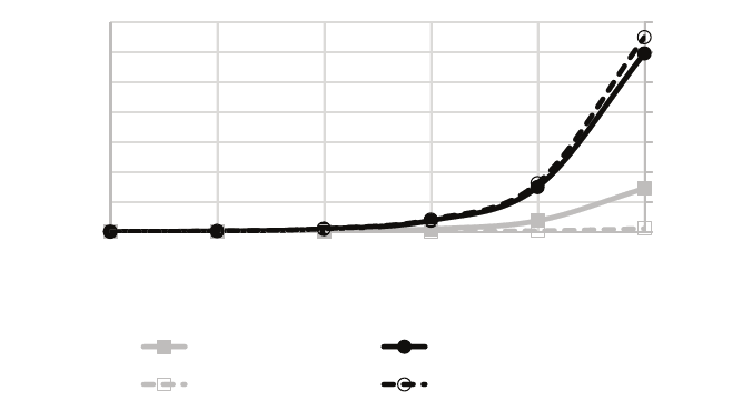
Scalability and sparsity. To understand the scalability of our protocols on large decision trees,

we perform a series of experiments on synthetic decision trees with diﬀerent depths and densities.

We ﬁrst consider complete decision trees, which serve as a “worst-case” bound on the protocol’s

performance for trees of a certain depth. In our experiments, we ﬁx the dimension of the feature

space to n = 16 and the precision to t = 64. We measure both the computation time and the total

communication between the client and server. Our results are shown in Figure 3. We note that

even for large trees with over ten thousand decision nodes, our protocol still operates on the order

of minutes.

We also compare our protocol against the private decision tree evaluation protocol of Brickell et

al. [20]. Their protocol can evaluate a 1100 node tree in around 5 minutes and 25 MB of communi-

cation. On a similarly sized tree over an equally large feature space, our protocol completes in 30

seconds and requires about 10 MB of communication, representing a 10x and a 2.5x improvement

in computation and bandwidth, respectively.

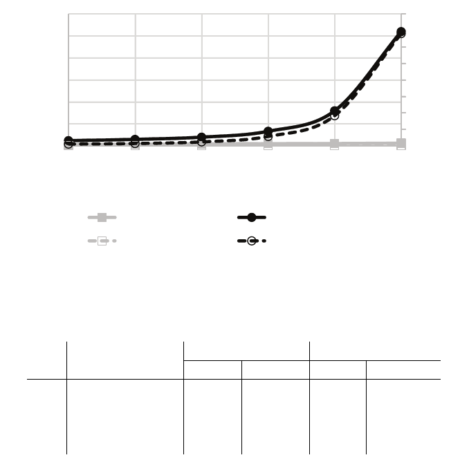
We also perform a set of experiments on “sparse” trees where the number m of decision nodes is

linear in the depth d of the tree. Here, we set m = 25d. We present the results of these experiments

in Figure 4. The important observation here is that the client’s computation now grows linearly,

rather than exponentially in the depth of the tree. Unfortunately, because the server computes a

decision string for the complete tree, the server’s computation increases exponentially in the depth.

However, since the cost of the homomorphic operations in the comparison protocol is greater than

the cost of computing the decision string, the protocol still scales to deeper trees and maintains

100

120

140

100

150

200

250

300

350

4 6 8 10 12 14

Bandwidth (MB)

Computaon Time (s)

Depth of Decision Tree

Client Computaon Server Computaon

Client Upload Server Upload

Figure 3: Client and server computation (excluding network communication) and total bandwidth

for semi-honest protocol on complete decision trees.

runtimes on the order of minutes. The limiting factor in this case is the exponential growth in

the size of the server’s response. Even though the tree is sparse, because the decision string

communicated by the server encodes information about every node in the padded tree, the amount

of communication from the server to the client is mostly unchanged. The communication upstream

from the client to the server, though, is signiﬁcantly reduced (linear rather than exponential in the

depth).

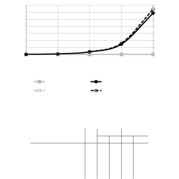
Handling malicious adversaries. Next, we consider the performance of the protocol from Fig-

ure 2 that provides protection against malicious adversaries. Since this protocol does not distinguish

between dummy and non-dummy nodes, the performance is independent of the number of actual

decision nodes in the tree. Thus, we only consider the benchmark for complete trees. Again, we

ﬁx the dimension n = 16 and the precision t = 64. The results are shown in Figure 5. Here,

the client’s computation grows linearly in the depth of the tree, and thus, is virtually constant in

these experiments. In all experiments in Figure 5, the total client-side computation is under half

a second. Moreover, the amount of communication from the client to the server depends only on

n, t, and is independent of the size of the model. Thus, the client’s computation is very small. This

means that the protocol is suitable for scenarios where the client’s computational power is limited.

The trade-oﬀ is that the server now performs more work. Nonetheless, even for trees of depth 12

(with more than 4000 decision nodes), the protocol completes in a few minutes. It is also worth

noting that this protocol is almost non-interactive (i.e., the client does not have to remain online

during the server’s computation).

As a ﬁnal note, we also benchmarked the protocol in Figure 2 on the ECG and Nursery datasets.

On the ECG dataset, the client’s and server’s computation took 0.191 s and 0.948 s, respectively,

with a total communication of 660 KB. On the Nursery dataset, the client’s and server’s compu-

tation took 0.216 s and 0.937 s, respectively, with a total communication of 720 KB. Even in spite

of the higher security level and the stronger security guarantees, our protocol remains 2x faster

100

120

140

160

100

120

10 12 14 16 18 20

Bandwidth (MB)

Computaon Time (s)

Depth of Decision Tree

Client Computaon Server Computaon

Client Upload

Server Upload

Figure 4: Client and server computation (excluding network communication) and total bandwidth

for semi-honest protocol on “sparse” trees.

k End-to-End (s)

Computation (s) Bandwidth (MB)

Client Server Client Server

10 26.161 4.652 19.069 0.247 9.106

25 65.067 11.343 47.756 0.430 22.761

50 130.496 22.252 95.133 0.736 45.520

100 256.362 44.759 190.196 1.346 91.037

Table 2: Semi-honest random forest evaluation benchmarks. Each forest consists of k trees (each

tree has depth at most 10 and exactly 100 comparisons). The “End-to-End” measurements include

the time for network communication.

than that of [17] in total computation time and requires 3.5x less communication. Thus, even the

protocol secure against malicious adversaries is practical, and for the reasons mentioned above (low

client overhead and only two rounds of interaction), might, in some cases, be more suitable than

the semi-honest secure protocol.

Random forests. As described in Section 5, we generalize our decision tree evaluation protocol

to support random forests with an aﬃne aggregation function with almost no additional overhead

than the cost of evaluating each decision tree privately. The computational and communication

complexity of the random forest evaluation protocol is just the complexity of the decision tree eval-

uation protocol scaled up by the number of trees in the forest. We give some example performance

numbers for evaluating a random forest with diﬀerent number of trees. Each tree in the forest

has depth at most 10 and contains exactly 100 comparisons. As before, we take n = 16 for the

dimension and t = 64 for the precision. Our results are summarized in Table 2.

100

120

140

100

150

200

250

300

350

4 6 8 10 12

Bandwidth (MB)

Computaon Time (s)

Depth of Decision Tree

Client Computaon Server Computaon

Client Upload Server Upload

Figure 5: Client and server computation (excluding network communication) and total bandwidth

for one-sided secure protocol for decision tree evaluation.

Dataset n

Tree Forest

d m d m

breast-cancer 9 8 12 11 276

heart-disease 13 3 5 8 178

housing 13 13 92 12 384

credit-screening 15 4 5 9 349

spambase 57 17 58 16 603

Table 3: Parameters for decision trees and random forests trained on UCI datasets [6]: n is the

dimension of the data, m is the number of decision nodes in the model, d is the depth of the tree(s)

in the model.

Performance on real datasets. We conclude our analysis by describing experiments on decision

trees and random forests trained on real datasets. We benchmark our protocol on ﬁve datasets

from the UCI repository [6] spanning application domains such as breast cancer diagnosis and

credit rating classiﬁcation. We train our trees using standard Matlab tools (classregtree and

TreeBagger). To obtain more robust models, we introduce a hyperparameter α ≥ 1 that speciﬁes

the minimum number of training examples that must be associated with each leaf node in the tree.

We choose α by running 10-fold cross validation [43] for several candidate values of α. In most

cases, α > 1, which has an added beneﬁt of reducing the depth of the resulting model. Additionally,

for two of the datasets (housing and spambase), we choose the best value for α such that the depth

of the resulting trees and forests is within 20. The size and depth of the resulting trees and forests,

along with the dimension of the feature space for each of the datasets is given in Table 3.

Of the ﬁve datasets we use for the benchmarks, four are binary classiﬁcation tasks. The excep-

tion is the housing dataset which is a regression problem. The heart-disease and credit-screening

datasets incorporate a mix of categorical and numeric variables. In our experiments, we operate

Dataset

Total Bandwidth (KB)

Time (s) Upload Download

breast-cancer 0.545 73.7 132.0

heart-disease 0.370 73.3 43.9

housing 4.081 115.7 1795.2

credit-screening 0.551 49.9 45.0

spambase 16.595 463.4 17363.3

Table 4: Performance (with network communication) of semi-honest decision tree evaluation pro-

tocol on UCI datasets.

Dataset

Total Bandwidth (KB)

Time (s) Upload Download

breast-cancer 9.671 106.7 4853.1

heart-disease 4.691 94.9 1758.2

housing 15.152 152.2 8357.4

credit-screening 8.737 92.9 3456.5

spambase 93.276 531.6 89310.7

Table 5: Performance (with network communication) of semi-honest random forest evaluation

protocol on UCI datasets [6].

at a 128-bit security level, and use 64 bits of precision to represent each component of the feature

vector. For the random forest experiments, we train a random forest consisting of 10 decision trees,

again choosing α via 10-fold cross-validation. The performance of the semi-honest decision tree

evaluation protocol on each of the ﬁve datasets is summarized in Table 4 and the performance

of the semi-honest random forest evaluation protocol is summarized in Table 5. We remark that

while our random forest extension only applies to aﬃne aggregation functions which are suitable

for regression problems and not classiﬁcation problems in general, our classiﬁcation examples are

all examples of binary classiﬁcation, in which case, taking the mean response is appropriate.

The performance benchmarks demonstrate that our semi-honest secure protocols are suitable

for evaluating trees and forests that could arise in practice. Even for relatively deep trees over high-

dimensional features spaces such as the spam classiﬁcation (spambase) dataset, our semi-honest

protocol completes in under 20 seconds. In all cases, the client’s computation time in the semi-

honest setting is under a second. For all but the largest tree (spambase), the total bandwidth is

under 2 MB. For smaller trees, the bandwidth is usually on the order of 100-200 KB. With random

forest evaluation, both the client and server have to perform additional computation and there is

more data exchanged. Nonetheless, the amount of computation required from the client is on the

order of a few seconds, and the server’s computation is also on the order of seconds (except in

the case of spambase where the computation took over a minute). Excluding spambase, the total

amount of communication is small.

Because we did not implement the extension to categorical variables for the protocol robust

against malicious adversaries, we do not have complete benchmarks for all ﬁve datasets. We

do have concrete results for the housing and breast-cancer datasets. On the breast-cancer

dataset, end-to-end decision tree evaluation using the protocol completes in 12.3 s including network

communication (client computation of just 0.263 s) and 8.2 MB of total communication. For the

housing dataset, the decision tree evaluation completes in 357.0 s (client computation of 0.384

s) and 256 MB of communication. These results indicate that for low-depth trees (d < 10), the

protocol in Figure 2 remains viable, but the amount of communication does grow rapidly in the

depth of the tree.

Comparison to generic methods. Private decision tree evaluation falls under the general

umbrella of secure two-party computation. While secure two-party computation protocols based

on Yao’s garbled circuits [63, 53] have seen numerous optimizations in the last several years [50, 51,

9, 64], a key limitation of these protocols has been bandwidth. We now describe a simple protocol

for private decision tree evaluation based on garbled circuits. In typical two-party computation

protocols, the function that is being evaluated is assumed to be public. In our setting, however, we

want to hide the structure of the decision tree from the client. Thus, we instead securely evaluate

a general decision tree evaluation circuit, which takes as input a description of a decision tree T

(from the server) and a feature vector x (from the client), and outputs T (x). This approach can

be viewed as securely evaluating a universal circuit for decision trees of up to depth d.

To compare our protocols to a generic protocol, we provide an estimate on the size of the

decision tree evaluation circuit. In the actual protocol execution, the server would send the client

a garbled version of this circuit together with the encodings of its input (the description of the

decision tree). The client then OTs for the encodings of its input wires (its feature vector), and

evaluates the circuit to learn the output. Because the decision tree evaluation circuit must support

evaluation of arbitrary trees of depth d, its size is lower bounded by the size of the circuit needed

to evaluate on a worst-case input (a complete decision tree of depth d). Using the state-of-the-art

free-XOR [51] and half-gate [64] optimizations for garbled circuits, the communicate required to

securely evaluate a garbled circuit depends only on the number of AND gates.

The circuit needed to evaluate a tree with depth d must perform 2

− 1 comparisons between

two t-bit values. Moreover, each comparison requires indexing into a feature vector of dimension

n (to select the value to be compared). Using the optimized comparison circuit from [50, §3.2],

comparing two t-bit integers can be performed using a circuit with exactly t AND gates. Using the

multiplexer circuits from [50, §C], selecting a t-bit value from a vector containing n such t-bit values

can be done using a circuit with (n − 1) · t AND gates. Thus, each comparison can be computed

with a circuit containing t + (n − 1) · t = n · t gates. Evaluating all of the comparisons in a complete

tree of depth d requires a circuit with at least (2

− 1) · n · t AND gates. Finally, computing the

output requires selecting one of 2

possible output values. If each output value has `-bits and using

the same multiplexer circuit as above, this step requires another (2

− 1) · ` AND gates. These

components give a conservative lower bound of (2

− 1)(nt + `) on the number of AND gates in the

circuit needed to generically evaluate a complete decision tree of depth d.

Using the half-gates optimization [64], each garbled AND gate requires sending a table that

contains exactly two rows, each λ bits long (where λ is the security parameter). At a 128-bit

security level, this means the size of a garbled circuit containing N AND gates is 32N bytes. Note

that the size of the garbled circuit provides only a lower bound on the total required communication

in Yao’s protocol. We neglect the interaction between the client and the server for the OTs. We

compare the communication required in our protocol with our estimates in Table 6 (with the

conservative estimate ` = 1).

In all cases, our semi-honest decision tree evaluation protocol requires less communication com-

Dataset

Bandwidth (KB)

Our Protocol Generic 2PC

breast-cancer 205.7 ≥ 4598.0

heart-disease 117.2 ≥ 182.2

housing 1910.9 ≥ 2.1 × 10

credit-screening 94.9 ≥ 450.5

spambase 17826.7 ≥ 1.5 × 10

Table 6: Bandwidth comparison between our proposed semi-honest protocol and estimated band-

width using a generic two-party computation protocol on trees trained from UCI datasets.

pared to our estimates for the bandwidth required by a generic Yao-based approach. This is because

in order to hide the structure of the tree, the generic approach necessarily incurs the worst-case

performance. As a result, the communication grows much more rapidly in the depth of the tree, and

quickly becomes infeasible. However, the generic solution does not reveal the number of internal

comparison nodes in the tree, while our semi-honest protocol does. It is worth noting that even for

complete decision trees, the bandwidth requirements of our protocol is still less than that required

by the generic solution.

In recent years, other generic two-party computation frameworks have been introduced that

combine Yao’s protocol with methods such as homomorphic encryption or secret sharing tech-

niques [12, 30]. Like Yao’s protocol, these generic tools can be leveraged for private decision tree

evaluation. However, as our above analysis shows, even for shallow decision trees, a generic circuit

for private decision tree evaluation is large and deep (due to the numerous comparison and multi-

plexing operations). Thus, direct application of these methods would likely lead to protocols with

higher bandwidth or require additional rounds of interaction.

7 Related Work

The earliest work for private decision tree evaluation focused on training decision trees in a privacy-

preserving manner [3, 52, 31]. In the case of [52, 31] multiple parties each have their own individual

datasets, and the objective is to compute a decision tree on their joint data without revealing their

individual datasets.

On the contrary, this work focuses on the problem of privately evaluating decision trees, where

it is assumed that one of the parties holds a trained decision tree or random forest. In [7, 20],

the authors develop protocols for privately evaluating linear branching programs (of which decision

trees are a special case) based on a combination of homomorphic encryption and garbled circuits.

Because these protocols solve a more general problem of evaluating linear branching programs,

they are not as competitive in performance in comparison to our protocol which exploits the simple

structure of decision trees. More recently, the work of [17] describes a fairly generic protocol for

decision tree evaluation that also splits up the decision tree evaluation protocol into two components:

a comparison phase followed by an evaluation phase. In [17], Bost et al. view the decision tree as a

polynomial in the decision variable and evaluate the polynomial using a SWHE scheme [35, 18, 41].

In all of these works, the authors achieve semi-honest security, although [20, 7] note that their

protocols can be made secure in the malicious setting without much diﬃculty. Nonetheless, we

do not know of any existing implementations of a private decision tree evaluation protocol that

achieves stronger security.

On the theoretical side, private decision tree evaluation falls into the category of private function

evaluation (where we view the decision tree as the underlying private function to be evaluated). In

the last few years, several generic approaches for private function evaluation have been proposed [47,

55] which are asymptotically very eﬃcient and can be made robust against malicious adversaries.

Restricting to private decision tree evaluation, Mohassel et al. describe a protocol for evaluating

oblivious decision programs based on OT in [54]. They provide an abstract method for evaluating

decision programs in both the semi-honest and malicious setting. However, it is unclear how to

integrate comparisons eﬃciently into their protocol, which would be necessary for evaluating the

particular kind of decision trees considered in this work. While the protocols of [47, 55, 54] apply

to our setting, we are not aware of any existing implementations of these methods.

8 Conclusion

In this work, we presented two protocols for privately evaluating decision trees and random forests.

The ﬁrst protocol based on additive homomorphic encryption and oblivious transfer is secure against

semi-honest adversaries. Then, using a novel conditional OT protocol, we showed how to modify

the protocol to obtain security against malicious adversaries. We implemented both protocols

and evaluated their performance on decision trees trained on several real-world datasets. Our

experiments demonstrate that our protocol is more eﬃcient in terms of both computation and

communication compared to existing protocols [7, 17]. A basic back-of-the-envelope calculation

shows that our protocols are much more eﬃcient in terms of communication compared to a generic

solution based on garbled circuits.

We leave as an open problem that of designing a private decision tree evaluation protocol whose

overall complexity is subexponential in the depth of the tree (i.e., a protocol whose performance is

not worst-case bounded). Another interesting direction is to explore how to eﬃciently update the

decision tree (or random forest) in a privacy-preserving manner.

Acknowledgments

We thank Melissa Chase, Seny Kamara, and Payman Mohassel for many helpful comments and

discussions on this work. The ﬁrst author is supported in part by an NSF Graduate Research

Fellowship under grant number DGE-114747 and an Amazon AWS in Education Grant.

References

[1] BigML. https://bigml.com/.

[2] Microsoft Azure Machine Learning. https://azure.microsoft.com/en-us/services/

machine-learning.

[3] R. Agrawal and R. Srikant. Privacy-preserving data mining. SIGMOD Rec., 29(2), 2000.

[4] G. Asharov, Y. Lindell, T. Schneider, and M. Zohner. More eﬃcient oblivious transfer and

extensions for faster secure computation. In CCS, pages 535–548, 2013.

[5] A. T. Azar and S. M. El-Metwally. Decision tree classiﬁers for automated medical diagnosis.

Neural Computing and Applications, 23(7-8):2387–2403, 2013.

[6] K. Bache and M. Lichman. UCI machine learning repository, 2013.

[7] M. Barni, P. Failla, V. Kolesnikov, R. Lazzeretti, A. Sadeghi, and T. Schneider. Secure

evaluation of private linear branching programs with medical applications. In ESORICS,

pages 424–439, 2009.

[8] M. Bellare and O. Goldreich. On deﬁning proofs of knowledge. In CRYPTO, pages 390–420,

1992.

[9] M. Bellare, V. T. Hoang, S. Keelveedhi, and P. Rogaway. Eﬃcient garbling from a ﬁxed-key

blockcipher. In IEEE Symposium on Security and Privacy, pages 478–492, 2013.

[10] M. Bellare, V. T. Hoang, and P. Rogaway. Foundations of garbled circuits. Cryptology ePrint

Archive, Report 2012/265, 2012.

[11] I. F. Blake and V. Kolesnikov. Strong conditional oblivious transfer and computing on intervals.

In ASIACRYPT, 2004.

[12] D. Bogdanov, S. Laur, and J. Willemson. Sharemind: A framework for fast privacy-preserving

computations. In ESORICS, pages 192–206, 2008.

[13] D. Boneh. The decision Diﬃe-Hellman problem. In ANTS, pages 48–63, 1998.

[14] J. Bos, C. Costello, P. Longa, and M. Naehrig. Speciﬁcation of curve selection and supported

curve parameters in MSR ECCLib. Technical Report MSR-TR-2014-92, Microsoft Research,

June 2014.

[15] J. W. Bos, C. Costello, P. Longa, and M. Naehrig. Selecting elliptic curves for cryptography:

An eﬃciency and security analysis. IACR Cryptology ePrint Archive, 2014:130, 2014.

[16] J. W. Bos, K. E. Lauter, and M. Naehrig. Private predictive analysis on encrypted medical

data. Journal of Biomedical Informatics, 50:234–243, 2014.

[17] R. Bost, R. A. Popa, S. Tu, and S. Goldwasser. Machine learning classiﬁcation over encrypted

data. In NDSS, 2015.

[18] Z. Brakerski, C. Gentry, and V. Vaikuntanathan. (Leveled) fully homomorphic encryption

without bootstrapping. In ITCS, pages 309–325, 2012.

[19] L. Breiman. Random forests. Machine Learning, 45(1):5–32, 2001.

[20] J. Brickell, D. E. Porter, V. Shmatikov, and E. Witchel. Privacy-preserving remote diagnostics.

In CCS, pages 498–507, 2007.

[21] J. Camenisch and M. Stadler. Eﬃcient group signature schemes for large groups (extended

abstract). In CRYPTO, pages 410–424, 1997.

[22] R. Canetti. Security and composition of multiparty cryptographic protocols. J. Cryptology,

13(1):143–202, 2000.

[23] R. Canetti. Security and composition of cryptographic protocols: a tutorial (part I). SIGACT

News, 37(3):67–92, 2006.

[24] D. Chaum and T. P. Pedersen. Wallet databases with observers. In CRYPTO, pages 89–105,

1992.

[25] R. Cramer, I. Damg˚ard, and B. Schoenmakers. Proofs of partial knowledge and simpliﬁed

design of witness hiding protocols. In CRYPTO, pages 174–187, 1994.

[26] R. Cramer, R. Gennaro, and B. Schoenmakers. A secure and optimally eﬃcient multi-authority

election scheme. In EUROCRYPT, pages 103–118, 1997.

[27] G. D. Crescenzo, R. Ostrovsky, and S. Rajagopalan. Conditional oblivious transfer and timed-

release encryption. In EUROCRYPT, pages 74–89, 1999.

[28] I. Damg˚ard, M. Geisler, and M. Krøigaard. Eﬃcient and secure comparison for on-line auctions.

In ACISP, pages 416–430, 2007.

[29] I. Damg˚ard, M. Jurik, and J. B. Nielsen. A generalization of Paillier’s public-key system with

applications to electronic voting. Int. J. Inf. Sec., 9(6):371–385, 2010.

[30] D. Demmler, T. Schneider, and M. Zohner. ABY - A framework for eﬃcient mixed-protocol

secure two-party computation. In NDSS, 2015.

[31] W. Du and Z. Zhan. Building decision tree classiﬁer on private data. In CRPIT ’14, 2002.

[32] Z. Erkin, M. Franz, J. Guajardo, S. Katzenbeisser, I. Lagendijk, and T. Toft. Privacy-

preserving face recognition. In PETS, pages 235–253, 2009.

[33] A. Fiat and A. Shamir. How to prove yourself: Practical solutions to identiﬁcation and

signature problems. In CRYPTO, pages 186–194, 1986.

[34] M. Fredrikson, S. Jha, and T. Ristenpart. Model inversion attacks that exploit conﬁdence

information and basic countermeasures. In ACM SIGSAC, pages 1322–1333, 2015.

[35] C. Gentry. A fully homomorphic encryption scheme. PhD thesis, Stanford University, 2009.

[36] O. Goldreich. Foundations of Cryptography: Volume 2, Basic Applications. Cambridge Uni-

versity Press, New York, NY, USA, 2004.

[37] S. Goldwasser and S. Micali. Probabilistic encryption. Journal of Computer and System

Sciences, 28(2):270–299, April 1984.

[38] S. Goldwasser, S. Micali, and C. Rackoﬀ. The knowledge complexity of interactive proof-

systems (extended abstract). In ACM STOC, pages 291–304, 1985.

[39] T. Graepel, K. E. Lauter, and M. Naehrig. ML conﬁdential: Machine learning on encrypted

data. In ICISC, pages 1–21, 2012.

[40] T. Granlund and the GMP development team. GNU MP: The GNU Multiple Precision Arith-

metic Library, 5.0.5 edition, 2012. http://gmplib.org/.

[41] S. Halevi and V. Shoup. Algorithms in HElib. In CRYPTO, pages 554–571, 2014.

[42] J. H˚astad, R. Impagliazzo, L. A. Levin, and M. Luby. A pseudorandom generator from any

one-way function. SIAM J. Comput., 28(4):1364–1396, 1999.

[43] T. Hastie, R. Tibshirani, and J. Friedman. The Elements of Statistical Learning. Springer

Series in Statistics. Springer New York Inc., 2001.

[44] C. Hazay and Y. Lindell. Eﬃcient Secure Two-Party Protocols - Techniques and Constructions.

Information Security and Cryptography. Springer, 2010.

[45] B. A. Huberman, M. K. Franklin, and T. Hogg. Enhancing privacy and trust in electronic

communities. In EC, pages 78–86, 1999.

[46] Y. Ishai, J. Katz, E. Kushilevitz, Y. Lindell, and E. Petrank. On achieving the ”best of both

worlds” in secure multiparty computation. SIAM J. Comput., 40(1):122–141, 2011.

[47] J. Katz and L. Malka. Constant-round private function evaluation with linear complexity. In

ASIACRYPT, pages 556–571, 2011.

[48] J. Kilian. Founding cryptography on oblivious transfer. In STOC, pages 20–31, 1988.

[49] H. C. Koh, W. C. Tan, and C. P. Goh. A two-step method to construct credit scoring models

with data mining techniques. International Journal of Business and Information, 1:96–118,

2006.

[50] V. Kolesnikov, A.-R. Sadeghi, and T. Schneider. Improved garbled circuit building blocks and

applications to auctions and computing minima. Cryptology ePrint Archive, Report 2009/411,

2009.

[51] V. Kolesnikov and T. Schneider. Improved garbled circuit: Free XOR gates and applications.

In ICALP, pages 486–498, 2008.

[52] Y. Lindell and B. Pinkas. Privacy preserving data mining. In CRYPTO, pages 36–54, 2000.

[53] Y. Lindell and B. Pinkas. A proof of security of Yao’s protocol for two-party computation. J.

Cryptology, 22(2):161–188, 2009.

[54] P. Mohassel and S. Niksefat. Oblivious decision programs from oblivious transfer: Eﬃcient

reductions. Financial Cryptography, 2014:269–284, 2012.

[55] P. Mohassel and S. S. Sadeghian. How to hide circuits in MPC: An eﬃcient framework for

private function evaluation. In EUROCRYPT, pages 557–574, 2013.

[56] M. Naor and B. Pinkas. Oblivious transfer and polynomial evaluation. In STOC, pages 245–

254, 1999.

[57] M. Naor and B. Pinkas. Eﬃcient oblivious transfer protocols. In SODA, pages 448–457, 2001.

[58] A. Narayanan, N. Thiagarajan, M. Lakhani, M. Hamburg, and D. Boneh. Location privacy

via private proximity testing. In NDSS, 2011.

[59] P. Paillier. Public-key cryptosystems based on composite degree residuosity classes. In EU-

ROCRYPT, volume 1592, pages 223–238. 1999.

[60] M. O. Rabin. How to exchange secrets with oblivious transfer. IACR Cryptology ePrint

Archive, 2005:187, 2005.

[61] V. Shoup. NTL: A library for doing number theory. http://www.shoup.net/ntl/.

[62] A. Singh and J. V. Guttag. A comparison of non-symmetric entropy-based classiﬁcation trees

and support vector machine for cardiovascular risk stratiﬁcation. Annual International Con-

ference of the IEEE Engineering in Medicine and Biology Society, pages 79–82, 2011.

[63] A. C. Yao. How to generate and exchange secrets (extended abstract). In FOCS, pages

162–167, 1986.

[64] S. Zahur, M. Rosulek, and D. Evans. Two halves make a whole - reducing data transfer in

garbled circuits using half gates. In EUROCRYPT, pages 220–250, 2015.

A Proof of Theorem 3.2

As described in Section 2.3, our decision tree evaluation protocol assumes that the following quan-

tities are public and known to both the client and the server in the protocol execution: the depth d

of the decision tree, the number of comparisons `, the dimension n of the feature vectors, and the

number of bits t needed to encode each component of the feature vector. To simplify the security

proof, we work in the OT-hybrid model where we assume that the client and server have access

to an ideal 1-out-of-2

OT functionality [48]. Speciﬁcally, in the real protocol, we replace the ﬁnal

OT invocation with an oracle call to a trusted party that implements the OT functionality: the

sender sends its database of 2

values (v

, . . . , v

) and the receiver sends an index i ∈ [2

] to the

trusted party. The trusted party then gives the receiver the value v

to the receiver. Security in

the standard model then follows by instantiating the ideal OT functionality with an OT proto-

col that provides security against semi-honest clients [56, 57] and invoking the sequential protocol

composition theorem of Canetti [22].

Security against a semi-honest server. First, we prove security against a semi-honest server.

Intuitively, security against a semi-honest server follows from the fact that the server’s view of the

protocol execution consists only of ciphertexts, and thus, reduces to a semantic security argument.

We now give the formal argument. Let A be a semi-honest server in the real protocol. We construct

an ideal-world simulator S as follows:

1. At the beginning of the protocol execution, the simulator S receives the input T from the

environment E. The simulator S sends the tree T to the trusted party.

2. The simulator starts running A on input T . Next, S generates a public-private key-pair

(pk, sk) for the additive homomorphic encryption scheme used in the protocol execution.

Then, S computes and sends nt fresh encryptions Enc

(0) of 0 to the server.

3. After A replies with the results of the comparison protocol, S computes and sends ` fresh

encryptions Enc

(0) of 0 to A.

4. The simulator outputs whatever A outputs.

We argue that REAL

π,A,E

(λ)

≈ IDEAL

π,S,E

(λ). By Theorem 3.1 and the fact that A is semi-honest,

we have that at the end of the protocol execution in the real world, the client obtains T (x) where x

is the client’s input. By deﬁnition of the ideal functionality, the trusted party computes T (x) and

gives it to the client. Thus, the client’s output in the real and ideal distributions are identically

distributed. Next, since the value T (x) is a deterministic function in the inputs T and x, the joint

distribution of the client’s output and the adversary’s output decomposes. To complete the proof,

it thus suﬃces to show that the view S simulates for A is computationally indistinguishable from

the view of A interacting in the real protocol.

The view of A in the real protocol consists of two components: the encryptions {Enc

i,j

)}

i∈[n],j∈[t]

of each bit of the client’s input and the encrypted bit string {Enc(b

)}

i∈[`]

. When interacting with

the simulator S, adversary A sees nt independent encryptions of 0, followed by ` independent en-

cryptions of 0. By semantic security of the underlying public-key encryption scheme, the server’s

view when interacting with the client in the real scheme is computationally indistinguishable from

its view interacting with the simulator. Thus, the output distribution of A in the real world is

computationally indistinguishable from that in the ideal world. Security follows.

Security against a semi-honest client. Next, we prove security against a semi-honest client.

Let A be a semi-honest client in the real protocol. We construct a semi-honest simulator S in the

ideal world as follows:

1. At the beginning of the protocol execution, S receives the input x from the environment E.

The simulator sends x to the trusted party. The trusted party replies with a value ˆz.

2. The simulator starts running A on input x. Let pk be the client’s public key.

3. The simulator samples a random string ˆσ

←− {0, 1}

and a random bit-string b

←− {0, 1}

Then, for each k ∈ [`]:

• If b

= 0, the simulator samples a value ˆc

k,j

←− Z

for all j ∈ [t].

• If b

= 1, the simulator chooses a random index j

∗

←− [t] and sets ˆc

k,j

∗

= 0. For j 6= j

∗

it samples ˆc

k,j

←− Z

4. When A submits the encryption of its feature vector, the simulator replies with the collection

of ciphertexts {Enc

(ˆc

k,j

)}

k∈[`],j∈[t]

5. When A sends the encrypted bit string (Step 4), the simulator replies with the bitwise en-

cryption Enc

(ˆσ) of ˆσ.

6. When A sends an index to the ideal OT functionality, S simulates the response from the ideal

OT functionality with ˆz.

7. At the end of the simulation, S outputs whatever A outputs.

In the decision tree functionality, the server has no output. Thus, to show security against a semi-

honest client, it suﬃces to show that the output of S is computationally indistinguishable from the

output of A. We show that the view S simulates for A is computationally indistinguishable from

the view of A interacting in the real protocol.

The client’s view in the real protocol consists of three components: the encrypted comparison

bits ct

k,j

for all k ∈ [`] and j ∈ [t], the encrypted decision string Enc

(σ

), and the response z from

the trusted OT functionality. For all k ∈ [`] and j ∈ [t], let c

k,j

= Dec

(ct

k,j

) be the comparison

bit encrypted by ct

k,j

. We now show that

k,j

}

k∈[`],j∈[t]

, σ

, z

| {z }

view in real protocol

≈

{ˆc

k,j

}

k∈[`],j∈[t]

, ˆσ, ˆz

| {z }

simulated view

We reason about each component individually:

• By correctness of the protocol (Theorem 3.1), z = T (x) in the real protocol. In the view S

simulates, ˆz is the response from the trusted party, and so ˆz = T (x) = z.

• Consider the distribution of σ

in the real protocol. By construction, σ

= τ(σ ⊕ s). Since s

is chosen uniformly and independently of σ, σ ⊕ s is uniform over {0, 1}

and independent

of the other components. Since τ is just a permutation on the bits, σ

= τ(σ ⊕ s) remains

independently uniform over {0, 1}

, and also independent of the other components. Thus, σ

is distributed identically as ˆσ.

• Consider the distribution of the {c

k,j

}

k∈[`],j∈[t]

in the real protocol. These values are computed

according to Eq. (1) in Figure 1. Fix an index k ∈ [`] and consider the set of values {c

k,j

}

j∈[t]

By construction, at most one c

k,j

= 0. Let b

= 1 {∃j : c

k,j

= 0}. From the analysis of

the comparison protocol in [28, §4.1], we have that b

⊕ b

= 1 {x

< t

}. Since the server

chooses b

uniformly and independently of 1 {x

< t

}, the bit b

is also uniform over {0, 1}.

In particular this means that with equal probability, the set {c

k,j

}

j∈[t]

contains t uniformly

random elements of Z

or t − 1 uniformly random elements of Z

and one component equal to

0. Since the ciphertexts {c

k,j

}

j∈[t]

are randomly permuted in the real protocol, if {c

k,j

}

j∈[t]

contains an element c

k,j

∗

= 0, it follows that j

∗

is uniform in [t]. Finally, since each comparison

is processed independently, c

k,j

is independent of c

whenever k 6= k

. But this is precisely

the same distribution from which S samples the ˆc

k,j

, and so we conclude that {c

k,j

}

k∈[`],j∈[t]

≡

{ˆc

k,j

}

k∈[`],j∈[t]

We conclude that

k,j

}

k∈[`],j∈[t]

, σ

, z

≡

{ˆc

k,j

}

k∈[`],j∈[t]

, ˆσ, ˆz

, and so the view S simulates for

A is computationally indistinguishable from the view A sees in the real protocol. Correspondingly,

the output of S is computationally indistinguishable from the output of A, and security follows.

B Proof of Theorem 4.1

In this section, we complete our analysis of the correctness and security of the decision tree evalu-

ation protocol in Figure 2. First, we show that the protocol is correct.

Lemma B.1. If the client and server follow the protocol in Figure 2, then at the end of the protocol,

the client learns T (x).

Proof. In the protocol in Figure 2, for each internal node k ∈ [m] in the decision tree, the server is

eﬀectively running the comparison protocol from [28] twice, once with blinding factor s

= 0 and

once with s

= 1. As in the proof of Theorem 3.1, we can appeal to the analysis of the comparison

protocol from [28, §4.1] and conclude that the bits b

for k ∈ [m] that the client computes in the

real game satisfy the relation s

⊕ b

= 1



< t



. Next, let b

denote the bit string b

· · · b

Then, b

is the decision string of x on T

, and so the leaf with index φ(b

) (as deﬁned in Section 2.2)

in T

contains the value T

(x) = T (x). By construction of the protocol, for each k ∈ [m] if the

client sets b

= 1, then it is able to decrypt one of the entries in

(1)

and learn the key κ

k,1

Conversely, if the client sets b

= 0, then it is able to decrypt one of the entries in

(0)

and learn

k,0

. In particular, the client obtains keys κ

k,b

for all k ∈ [m]. This allows the client to compute

the value used to blind z

φ(b

)

in the blinded response vector and learn T (x).

Before proceeding with the proof of Theorem 4.1, we ﬁrst characterize the distribution of values in

the blinded response vector [ˆz

, . . . , ˆz

]. In particular, we show that for any bit string b ∈ {0, 1}

given the set of keys {κ

k,b

}

k∈[m]

corresponding to the bits of b, all but one entry in the blinded

response vector is uniformly random over Z

. More formally, take a complete binary tree T with

depth d. Let m = 2

−1 denote the number of internal nodes in T . For k ∈ [m], choose κ

k,0

, κ

k,1

←−

. Next, for i = 0, 1, . . . , m, let b

· · · b

be the binary representation of i, and let i

, . . . , i

be the

indices of the nodes in the path induced by b

· · · b

in T . Deﬁne z

to be

j∈[d]

h(κ

), (2)

where h is a pairwise independent hash function from Z

onto {0, 1}

(for some output length `

where ` < blog

pc). Intuitively, we associate a uniformly random key with each edge in T (or

equivalently, two keys with each internal node). The value z

is the xor of the keys associated with

each edge in the path from the root to leaf i. Now, we state the main lemma on the distribution of

each z

conditioned on knowing exactly one of the two keys associated with each internal node.

Lemma B.2. Fix a complete binary tree T with depth d. Let m = 2

− 1 and for each 0 ≤ i ≤ m,

construct z

according to Eq. (2) where κ

k,b

←− Z

for k ∈ [m] and b ∈ {0, 1}. Take any bit-string

b ∈ {0, 1}

and let α = φ(b) be the index of the leaf node in the path induced by b in T . Then, for

all i 6= α, the conditional distribution of z

given {κ

k,b

}

k∈[m]

is independent of the other entries

}

k6=i

and statistically close to uniformly random over {0, 1}

Proof. We argue by induction in the depth of the tree. When d = 1, there are exactly two keys κ

1,0

and κ

1,1

. Moreover, z

= h(κ

1,0

) and z

= h(κ

1,1

). Since κ

1,0

and κ

1,1

are independently uniform

over Z

, and h is pairwise independent, the claim follows by the leftover hash lemma.

For the inductive step, take a tree T of depth d > 1 and a bit-string b ∈ {0, 1}

. Let α be the

index of the leaf node in the path induced by b in T . Let

T be the complete subtree of T (rooted

at the same node) of depth d − 1. For i = 0, . . . , 2

d−1

, let

· · ·

d−1

be the binary representation

of i and let

, . . . ,

d−1

be the indices of the nodes in the path induced by

· · ·

d−1

T . Then,

deﬁne the value ˆz

j∈[d−1]

h(κ

). Set ˆm = 2

d−1

− 1, and

b = b

· · · b

d−1

. Let ˆα be the index

of the leaf node in the path induced by

b in

T . Invoking the induction hypothesis, we have that for

all i 6= ˆα, the conditional distribution of ˆz

given {κ

k,b

}

k∈[ ˆm]

is statistically close to the uniform

distribution on {0, 1}

and independent of the other components. In other words, conditioned on

the set {κ

k,b

}

k∈[ ˆm]

, we have that

[ˆz

, . . . , ˆz

ˆα−1

, ˆz

ˆα+1

, . . . , ˆz

ˆm

]

≈ [ˆr

, . . . , ˆr

ˆα−1

, ˆr

ˆα+1

, . . . , ˆr

ˆm

] , (3)

where ˆr

, . . . , ˆr

ˆm

are independently and uniformly random over {0, 1}

. Note that Eq. (3) holds

even if we condition over the full set of keys {κ

k,b

}

k∈[m]

, since ˆz

is independent of κ

k,b

for k > ˆm.

Each z

is deﬁned to be the xor of the hash of all the keys along the path from the root to the

leaf in T . We can decompose this as taking the xor of all the keys along the path from the

root to the parent of the i

leaf, and xoring with the key associated with the edge from the parent

to the leaf. Next, observe that the xor of the keys from the root to the parent of the i

leaf is

precisely ˆz

bi/2c

. Finally, let p

denote the index of the parent node of the i

leaf in T . Then,

j∈[d]

h(κ

) = ˆz

bi/2c

⊕ h(κ

) = ˆz

bi/2c

⊕ h(κ

,(i mod 2)

). (4)

We now show that [z

, . . . , z

α−1

, z

α+1

, . . . , z

]

≈ [r

, . . . , r

α−1

, r

α+1

, . . . , r

], where r

, . . . , r

are

independent and uniform in {0, 1}

. From Eq. (4), we can write z

= ˆz

bi/2c

⊕ κ

,(i mod 2)

. By

assumption, for each i ∈ [m], we are given exactly one of the keys κ

and κ

. Let A be the

subset of {z

}

i6=α

for which we know the the key κ

,(i mod 2)

, and let B be the subset of {z

}

i6=α

for

which we do not know the key κ

,(i mod 2)

. To complete the proof, we use a hybrid argument.

• First, we show that the conditional distribution of the elements of A and B (given the keys)

is statistically close to the conditional distribution of A and B

, where each element in B

uniform and independent over {0, 1}

To see this, take any z

∈ B. Since B contains the elements z

for which we are not given

the associated key κ

,(i mod 2)

, we can write z

as ˆz

⊕ h(κ

,1−b

), for some 0 ≤ i

≤ ˆm and

∈ [m]. Now, κ

,1−b

is independent and uniform over Z

, and in particular, independent

of {κ

k,b

}

k∈[m]

. Moreover, z

is the only element that depends on κ

,1−b

. Since h is sampled

from a pairwise independent family of hash functions, by the leftover hash lemma, h(κ

,1−b

)

is statistically close to uniform over {0, 1}

. The claim follows.

• Next, we show that the conditional distribution of A and B

(given the keys) is statistically

close to the conditional distribution of A

and B

, where each element in A

is uniform and

independent in {0, 1}

To see this, take any z

∈ A. We can write z

= ˆz

⊕ h(κ

) for some i

6= ˆα and k

∈ [m].

From Eq. (3), ˆz

is statistically close to uniform over {0, 1}

. Moreover, no other element in

A depends on ˆz

, so we conclude that z

is independent of all the other elements of A. Finally,

since the elements of B

are independent, uniform draws from {0, 1}

, z

is independent of all

the other elements in A and B

. Thus, the conditional distribution of A and B

is statistically

close to the conditional distribution of A

and B

, and the claim holds.

By induction on d, we conclude that for all i 6= α, the conditional distribution of z

given {κ

k,b

}

k∈[m]

is statistically close to uniform over {0, 1}

, and independent of z

for all j 6= i.

We now now ready to show that the protocol in Figure 2 provides security against a malicious client

and privacy against a malicious server. As described in Section 2.3, we assume the depth of the

decision tree d, the dimension n of the feature vector, and the precision t used to represent elements

of the feature vector are public and known to all parties. We also assume that the decision tree is

complete, so the number of internal nodes m is given by m = 2

− 1.

Privacy against a malicious server. Let A be a server. We construct a simulator S that

interacts only with the ideal functionality such that the output of the simulator is computationally

indistinguishable from the output of A in the real world. Our simulator S works as follows:

1. The environment gives an input T to the simulator.

2. The simulator starts running A on input T .

3. For each i ∈ [n] and j ∈ [t], S sets ˆx

i,j

= 0 and samples ˆr

i,j

←− Z

. It then constructs

ciphertexts

i,j

← Enc

(ˆx

i,j

; ˆr

i,j

) and associated proofs

ˆπ

i,j

← PoK



i,j

) :

i,j

= Enc (0; r

i,j

) ∨

i,j

= Enc (1; r

i,j

)



Note that these are the same Chaum-Pedersen style proofs used in the real protocol (Figure

2). The simulator gives the ciphertexts

i,j

and proofs bπ

i,j

to A.

4. Finally, S outputs whatever A outputs.

The view of the adversary A when interacting in the real protocol is computationally indistinguish-

able from its view when interacting with the simulator S. This is easy to see since the view of A

consists only of ciphertexts and the associated zero-knowledge proofs. By semantic security of the

underlying encryption scheme, and the zero-knowledge property of the proofs, we conclude that

the view of A in the two cases is computationally indistinguishable, and thus, the output of A in

the real scheme is computationally indistinguishable from the output of S in the ideal world.

Security against a malicious client. Next, we show security against a malicious client. Let A

be a PPT client in the real world. We construct our ideal-world simulator S as follows:

1. The environment gives an input x to S. The simulator starts running A on input x.

2. Algorithm A can abort, in which case, the simulator also aborts. Otherwise, algorithm A

produces a sequence of ciphertexts Enc(ˆx

i,j

; r

i,j

) and proofs π

i,j

that ˆx

i,j

∈ {0, 1} for all

i ∈ [m], j ∈ [t],

3. For each i ∈ [m], j ∈ [t], the simulator verify the proof π

i,j

. If any proof fails to verify, it

aborts the protocol, and outputs whatever A outputs. Otherwise, it applies the knowledge

extractor (from the proof of knowledge system) to π

i,j

to extract the randomness r

i,j

used to

encrypt each ˆx

i,j

. If the knowledge extractor fails, the simulator outputs ⊥. If the simulator

does note abort, then it learns each bit ˆx

i,j

of each component of the client’s input vector.

Denote the extracted client input by ˆx. The simulator sends ˆx to the TTP, and receives T (ˆx).

4. The simulator samples values ˆz

, . . . , ˆz

←− {0, 1}

as well as a random bit-string

←− {0, 1}

For each i ∈ [m], it additionally samples keys ˆκ

←− Z

. Let i

, . . . , i

be the indices of the

nodes in the path induced by

in a complete binary tree of depth d, and let ` be the

index of the leaf node at the end of the path induced by

The simulator updates ˆz

T (ˆx) ⊕



i∈[d]

h(ˆκ

)



, where h : G → {0, 1}

is drawn from the same pairwise independent

hash family (as in the real scheme).

5. Next, S simulates the sets of ciphertexts A

(0)

, A

(1)

, B

(0)

, B

(1)

from the real scheme. For each

k ∈ [m], the simulator does the following

(a) First, for j ∈ [t] and b ∈ {0, 1}, the simulator samples random values ˆc

(b)

k,j

←− Z

, and

(b)

k,j

←− Z

. Next, is chooses a random index index j

∗

←− [t], and updates ˆc

)

k,j

∗

= 0 and

)

k,j

∗

= ˆκ

(b) Next, the simulator constructs the tuples

(0)



Enc

(ˆc

(0)

k,1

), . . . , Enc

(ˆc

(0)

k,t

)



(0)



Enc

(

(0)

k,1

), . . . , Enc

(

(0)

k,t

)



(1)



Enc

(ˆc

(1)

k,1

), . . . , Enc

(ˆc

(1)

k,t

)



(1)



Enc

(

(1)

k,1

), . . . , Enc

(

(1)

k,t

)



The simulator sends the blinded response vector [ˆz

, . . . , ˆz

] and the sets of ciphertexts

(0)

(1)

(0)

(1)

for k ∈ [m] to A

6. At the end of the simulation, S outputs whatever A outputs.

We show that on input x from the environment, the output of the simulator S is computationally

indistinguishable from the output of A in the real world. Certainly, if A aborts the protocol before

sending any messages, then the simulator also aborts, so the behavior of A and S is identical up to

the end of Step 2 of the simulation. Next, if the simulator aborts the protocol because the proofs

fail to verify, then in the real protocol, the server would also abort the protocol (assuming the proof

system is sound). Thus, the behavior of the simulator up to this point is identical to the behavior

of the server in the real-world, and so, the outputs of the simulator are identically distributed as

the outputs of A.

Since the proofs verify, the knowledge extractor succeeds in extracting the client’s input x with

overwhelming probability. We now argue that the simulator’s response to A is computationally

indistinguishable from the server’s response to A in the real protocol. The adversary’s view in the

real protocol consists of the following components: the blinded response vector [z

, . . . , z

] and the

collections of ciphertexts A

(0)

, A

(1)

, B

(0)

, B

(1)

for k ∈ [m].

• First, we show that for all k ∈ [m], the ciphertexts (A

(0)

, A

(1)

, B

(0)

, B

(1)

) are distributed

identically as (

(0)

(1)

(0)

(1)

). In the real scheme, let c

(b)

k,j

be the values appearing in

(b)

for j ∈ [t] and b ∈ {0, 1}. By construction, for all k ∈ [m], there is an index j

∗

∈ [t] such

that either

– c

(0)

k,j

∗

= 0, and c

(1)

k,j

∗

is uniform over Z

, and for all j 6= j

∗

, b ∈ {0, 1}, c

(b)

k,j

is also uniform

over Z

. In this case, an honest client would compute b

= 0.

– c

(1)

k,j

∗

= 0, and c

(0)

k,j

∗

is uniform over Z

, and for all j 6= j

∗

, b ∈ {0, 1}, c

(b)

k,j

is also uniform

over Z

. In this case, an honest client would compute b

= 1.

Next, appealing again to the analysis of the comparison protocol from [28, §4.1], we have that

⊕ b

= 1



< t



. In the real scheme, the server samples the bit-string s uniformly at

random, and so the permuted bit-string s

is also uniform over {0, 1}

. This means that the

bit-string b

that the honest client would compute is distributed uniformly over {0, 1}

, and

so the two cases above occur with equal probability. But now this is exactly the distribution

from which the simulator samples the elements of

(0)

and

(1)

Next, consider the values in B

(0)

and B

(1)

in the real scheme. For all j ∈ [t], if A

(0)

k,j

6= 0, then

(0)

k,j

is uniform in Z

. The same is true of B

(1)

k,j

if A

(1)

k,j

6= 0. Once again, this is how the values

(0)

k,j

and

(1)

k,j

are constructed in the simulation (when

(0)

k,j

6= 0 and

(1)

k,j

6= 0). When A

(b)

k,j

= 0

for some j ∈ [t] and b ∈ {0, 1}, then B

(b)

k,j

= κ

k,b

in the real scheme, where κ

k,b

is uniform over

. In the simulation,

(b)

k,j

= ˆκ

when

(b)

k,j

= 0. Since κ

is also sampled uniformly from Z

we conclude that taken independently, the collections (A

(0)

, A

(1)

, B

(0)

, B

(1)

) are identically

distributed as (

(0)

(1)

(0)

(1)

• To conclude the proof, we argue that the conditional distribution of the blinded response

vector [z

, . . . , z

] in the real experiment is statistically indistinguishable from the simulated

response vector [ˆz

, . . . , ˆz

] in the ideal experiment. First, in the real protocol, the client is

able to recover κ

k,b

from B

)

. However, the client’s view of the protocol is independent

of κ

k,1−b

for all k ∈ [m]. The only components of the client’s view that depend on κ

k,1−b

are the elements in the set B

(1−b

)

. However, by construction, each of the values c

(1−b

)

k,j

non-zero, so in the real scheme, the value of κ

k,1−b

is information-theoretically hidden by the

blinding factor ρ

(1−b

)

k,j

∈ Z

. Thus, the client’s view is independent of κ

k,1−b

for all k ∈ [m].

Let i

∗

be the index of the leaf node in T induced by the bit-string b

. We can now invoke

Lemma B.2 to conclude that the conditional distribution of z

for all i 6= i

∗

is statistically

close to uniform over {0, 1}

. Moreover, by correctness of the protocol (Lemma B.1), we have

that z

∗

= T (x) ⊕

j∈[d]

h(κ

∗

), where x here is the input the client submitted to the server

at the beginning of the protocol execution (by soundness of the zero-knowledge proofs, we

are ensured that this is a valid input).

As argued before, the bit string

chosen in the simulation is distributed identically to the

bit-string b

the client would normally obtain in the real scheme. Thus, let

∗

be the index

of the leaf node in T induced by the bit-string

∗

. For all i 6= i

∗

, the simulator chooses the

entry ˆz

uniformly at random from {0, 1}

, which matches the distribution in the real scheme.

Finally, the simulator sets z

∗

= T (ˆx) ⊕

j∈[d]

h(ˆκ

). Here ˆx is the input extracted from

the client’s proofs of knowledge. Additionally, as argued earlier, for all k ∈ [m], ˆκ

in the

simulation is distributed exactly as κ

k,b

in the real protocol.

We conclude that the view of the adversary is computationally indistinguishable in the real and

ideal experiments. This suﬃces to prove security against a malicious client.