i
BUILDING A STATISTICAL LEARNING MODEL
FOR EVALUATION OF NBA PLAYERS USING
PLAYER TRACKING DATA
By
Matthew Byman, B.A. in Economics
A thesis submitted to the Graduate Committee of
Ramapo College of New Jersey in partial fulfillment
of the requirements for the degree of
Master of Science in Data Science
Spring, 2023
Committee Members:
Osei Tweneboah, Advisor
Debbie Yuster, Reader
Nikhil Varma, Reader
ii
COPYRIGHT
© Matthew Byman
2023
iii
Table of Contents
List of Figures ............................................................................................................................... v
Abstract ..................................................................................................................................... vii
Chapter 1: Introduction ................................................................................................................. 1
Chapter 2: Background .................................................................................................................. 5
History of Basketball Advanced Analytics ................................................................................ 5
Ordinary Least Squares (OLS) ................................................................................................ 7
Ridge Regression ..................................................................................................................... 8
Lasso Regression ....................................................................................................................10
Decision Tree .........................................................................................................................11
Random Forest ......................................................................................................................12
Regularized Adjusted Plus Minus (RAPM) .............................................................................14
Chapter 3: Methodology ...............................................................................................................17
Dataset Description ................................................................................................................19
Dataset cleaning .....................................................................................................................22
Distribution of RAPM and Correlation Matrix ........................................................................22
Co-efficient Estimation of Our Models ....................................................................................25
Training our Models ...............................................................................................................28
Deployment of our Models ......................................................................................................31
Chapter 4: Analysis and Discussion ...............................................................................................34
iv
Comparing our results ............................................................................................................34
Implications for NBA teams ....................................................................................................38
Limitations of our study .........................................................................................................39
Chapter 5: Conclusions ................................................................................................................42
Chapter 6: References ..................................................................................................................44
Appendix....................................................................................................................................46
v
List of Figures
Figure 2.1: An example of OLS graphed
Figure 2.2: Geometric Interpretation of Ridge Regression
Figure 2.3: Estimation picture of Lasso (left) and Ridge Regression (right)
Figure 2.4: Decision Tree’s 1 and 2 for the Random Forest model in this study
Figure 2.5: 3-year RAPM (2020-2023)
Figure 3.1: Flowchart of our methodology process
Figure 3.2: Distribution of RAPM (2021)
Figure 3.3: Correlation Matrix (2021)
Figure 3.4: OLS Co-efficient Estimation (2021)
Figure 3.5: Lasso Co-efficient Estimation (2021)
Figure 3.6: Ridge Co-efficient Estimation (2021)
Figure 3.7: Decision Tree Co-efficient Estimation (2021)
Figure 3.8: Random Forest Co-efficient Estimation (2021)
Figure 3.9: Top two models with all features included (2021)
Figure 3.10: Statistical models with top performing features (2021)
Figure 3.11: Top two performing models with all features against the 2022 testing data
Figure 3.12: Statistical models with top performing features against the 2022 testing data
Figure 4.1: Table of top two performing models metrics
Figure 4.2: Table of models metrics with top performing features
Figure 4.3: Table of top two performing models against 2022 data
Figure 4.4: Table of models metrics with top performing features against 2022 data
vi
Figure 4.5: 2022 RAPM Values vs 2022 Predicted RAPM Values with Lasso
Figure 4.6: 2022 RAPM metrics vs 2022 Predicted RAPM with Lasso metrics
vii
Abstract
This thesis aims to develop faster and more accurate methods for evaluating NBA player
performances by leveraging publicly available player tracking data. The primary research
question addresses whether player tracking data can improve existing performance evaluation
metrics. The ultimate goal is to enable teams to make better-informed decisions in player
acquisitions and evaluations.
To achieve this objective, the study first acquired player tracking data for all available NBA
seasons from 2013 to 2021. Regularized Adjusted Plus-Minus (RAPM) was selected as the target
variable, as it effectively ranks player value over the long term. Five statistical learning models
were employed to estimate RAPM using player tracking data as features. Furthermore, the
coefficients of each feature were ranked, and the models were rerun with only the 30 most
important features.
Once the models were developed, they were tested on a newly acquired player tracking data from
the 2022 season to evaluate their effectiveness in estimating RAPM. The key findings revealed
that Lasso Regression and Random Forest models performed the best in predicting RAPM
values. These models enable the use of player tracking statistics that settle earlier, providing an
accurate estimate of future RAPM. This early insight into player performance offers teams a
competitive advantage in player evaluations and acquisitions.
In conclusion, this study demonstrates that combining statistical learning models with player
tracking data can effectively estimate performance metrics, such as RAPM, earlier in the season.
viii
By obtaining accurate RAPM estimates before other teams, organizations can identify and
acquire top-performing players, ultimately enhancing their competitive edge in the NBA.
1
Chapter 1: Introduction
Basketball, one of the most popular and widely followed sports globally, has undergone
numerous transformations since its inception in the late 19th century. The game's history,
evolution, and the significance of analytics in the modern era are all critical aspects of
understanding the sport as we know it today.
In 1891, James Naismith, a 31-year-old graduate student at Springfield College, conceived
basketball as an engaging indoor sport to occupy his fellow students during the winter months
while they awaited the return of warmer weather for outdoor sports such as football, lacrosse,
and baseball ("Where Basketball Was Invented: The Birthplace of Basketball."). The initial
iteration of basketball diverged significantly from the contemporary version of the game,
featuring peach baskets as goals and nine players per team; nevertheless, the essence of
basketball remained. Professional leagues emerged shortly thereafter, with the National
Basketball League (NBL) being established in 1898. Although the NBL only endured for five
years, subsequent attempts to form professional leagues ensued. The National Basketball
Association (NBA) that we know today was ultimately established in 1949, following the merger
of the NBL and the Basketball Association of America ("History of Basketball Leagues."). The
sport has also become an essential feature of the Olympic Games, with its debut in the 1936
Berlin Olympics.
The earliest documented basketball statistics date back to the National Basketball League in
1946. At that time, local newspapers published rudimentary box scores the day following games,
2
which included field goals (baskets made during gameplay), free throws (uncontested shots taken
after an opposing player commits a foul), and individual points scored for each player on both
teams ("How Basketball-Reference Got Every Box Score."). Over the years, statistical analysis
in basketball has evolved dramatically, subsequently influencing the game's strategies and
overall style of play.
Basketball analytics, the use of advanced statistical analysis to evaluate team and player
performance, has revolutionized the sport over the past few decades. Traditionally, teams and
coaches relied on basic statistics, such as points, rebounds, and assists, to evaluate player
contributions. However, with the emergence of new analytical tools and methodologies, teams
now have access to more sophisticated metrics that offer deeper insights into a player's value.
In the early 2000s, the advent of player tracking technology, such as SportVU (SportVU is the
camera system that tracks player’s movements on the court), enabled the collection of detailed
spatial and temporal data on player movements, shot trajectories, and defensive positioning. This
wealth of data led to the development of new advanced metrics, including Player Efficiency
Rating (PER), Win Shares, and Real Plus-Minus (RPM) ("NBA Analytics Movement: How
Basketball Data Science Has Changed the Game."). These metrics allow teams and coaches to
make more informed decisions about roster construction, game strategy, and player development.
As the importance of analytics continues to grow, it will undoubtedly shape the future of the
sport, leading to new strategies, enhanced player development, and an even more competitive
and exciting game for fans worldwide. This thesis will attempt to use these player-tracking
technologies along with established statistical models to help drive the game of basketball
forward and improve on existing player evaluation techniques. At present, there is a lack of
3
research that integrates player tracking data with statistical models for player evaluation
purposes. The majority of existing NBA player assessment tools remain opaque, as their inner
workings are not disclosed to the public.
We will explore five popular statistical learning models: Ordinary Least Squares (OLS), Ridge
Regression, Lasso Regression, Decision Tree, and Random Forest. Each model has its unique
strengths and limitations, making them suitable for different types of problems and data sets.
After examining the inner workings of our models, we will delve into the methodology
employed in our study. This discussion will encompass the data selection process and the criteria
used for determining the most crucial features.
Ultimately, we will address the outcomes of our analysis and demonstrate how our model can be
utilized in the basketball industry to elevate existing benchmarks. By adopting this model, teams
can leverage its insights to drive success and gain a competitive edge.
An overview of our chapters in this study, in Chapter 2, we will provide a comprehensive
background to our study, delving into the history of basketball analytics and its transformative
impact on the modern sport. We will also present a thorough explanation of our five statistical
learning models, outlining their respective functionalities and justifying the selection of our
target variable.
In Chapter 3, we will detail our methodology, elucidating every step involved in our research
process. This will encompass a description of the dataset employed, the data cleaning process,
model training procedures, coefficient estimation techniques to identify crucial features, and,
ultimately, the deployment of our models.
4
In Chapter 4, we will present a critical analysis of our models, discussing the results obtained and
their implications. This chapter will further explore the potential effects of our model on NBA
team strategies, acknowledging the limitations of our study and suggesting possible
improvements for future research. We will also consider the broader implications of our findings
within the context of the sport and analytics.
Chapter 5 will present our conclusions and final thoughts, highlighting the key insights derived
from our study and identifying avenues for future work that could build upon and extend the
scope of our research.
5
Chapter 2: Background
We will first delve into the history of basketball analytics, past works, and why player tracking
cameras are such an evolution in the game of basketball. We will then discuss our five statistical
models and how each of them works. After that we will explain our target variable and why it
was chosen.
History of Basketball Advanced Analytics
The history of advanced basketball analytics in the modern era can be traced back to the early
2000s, when the sport began to adopt more sophisticated statistical methods to analyze and
evaluate player performance. The Moneyball revolution in baseball, spearheaded by Oakland
Athletics General Manager Billy Beane, had a profound impact on basketball, as teams and
analysts started to embrace data-driven approaches to gain a competitive edge ("NBA Analytics
Movement: How Basketball Data Science Has Changed the Game.").
In the early days of basketball analytics, pioneers such as Dean Oliver and John Hollinger
developed groundbreaking metrics like Offensive Rating, Defensive Rating, and Player
Efficiency Rating (PER) that went beyond traditional box score statistics. Oliver's seminal book,
"Basketball on Paper," published in 2004, laid the foundation for modern basketball analytics,
emphasizing the importance of efficiency and situational analysis.
The availability of play-by-play data and the rise of the internet allowed for the development of
new metrics, such as Adjusted Plus-Minus (APM) and its derivatives like Regularized Adjusted
Plus-Minus (RAPM), which account for the context of teammates and opponents on the court.
6
These metrics provided a more accurate measure of a player's impact on their team's
performance.
The introduction of SportVU player tracking technology in the NBA in 2013 marked a turning
point in basketball analytics, as it provided unprecedented access to spatial and temporal data,
capturing every movement of the players and the ball at a rate of 25 times per second ("The NBA
releases SportVU Camera Statistics."). This wealth of information enabled the development of
advanced metrics like Player Impact Estimate (PIE), Player Tracking Plus-Minus (PT-PM), and
Quantified Shot Quality (QSQ), which leveraged machine learning algorithms and spatial
analysis techniques to better understand player performance and decision-making.
Player tracking data has become an indispensable tool in basketball analytics for several reasons:
Granularity: Player tracking data provides detailed information about each player's movements
and actions on the court, allowing for more nuanced analysis of individual skills and tendencies.
Contextual Analysis: With player tracking data, analysts can study the impact of spatial
relationships, defensive pressure, and offensive spacing on player performance, leading to a
deeper understanding of the game's dynamics.
Load Management: By analyzing player movements and workload, teams can better manage
players' health and recovery, reducing the risk of injury and optimizing performance.
Game Planning: Access to detailed player tracking data enables coaches and analysts to develop
tailored game plans and strategies based on their opponents' strengths and weaknesses.
7
Player Development: The insights gained from player tracking data can help teams identify
areas for improvement and guide player development programs.
In conclusion, the modern era of basketball analytics has witnessed a rapid evolution, driven by
the adoption of data-driven approaches and the availability of advanced player tracking
technology. These innovations have transformed how teams evaluate players, develop strategies,
and manage player health, leading to a more sophisticated understanding of the game.
Ordinary Least Squares (OLS)
Ordinary Least Squares (OLS) is a fundamental linear regression method that aims to model the
relationship between a dependent variable and one or more independent variables ("Ordinary
Least Square (OLS) Method for Linear Regression."). In a linear regression model, the
dependent variable is assumed to be a linear function of the independent variables, plus some
random error component. The main objective of OLS is to find the best-fitting line that
minimizes the sum of the squared differences between the observed values of the dependent
variable and the predicted values based on the model.
To accomplish this, OLS estimates the coefficients of the independent variables by minimizing
the residual sum of squares (RSS). The residual for each observation is the difference between
the observed value of the dependent variable and the value predicted by the model. The RSS is
the sum of the squares of these residuals. By minimizing the RSS, OLS finds the optimal set of
coefficients that best explain the relationship between the independent and dependent variables.
8
OLS is a popular method due to its simplicity, interpretability, and ease of implementation. It
performs well when the relationship between the variables is linear, and there is little
multicollinearity. However, it can be sensitive to outliers and may perform poorly when the
independent variables are highly correlated, as it does not provide any regularization to prevent
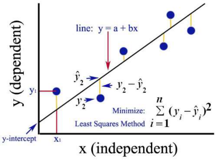
overfitting. Figure 2.1 shows how the OLS method seeks to minimize the residual sum of
squares and create a line of best fit.
Figure 2.1: An example of OLS graphed
Ridge Regression
Ridge Regression is an extension of linear regression that introduces a regularization term to
address the limitations of OLS. Regularization is a technique that adds a penalty to the regression

9
coefficients based on their magnitude, effectively shrinking the coefficients toward zero. This
helps to reduce overfitting, especially when there are many irrelevant or noisy features in the
data, and to handle multicollinearity.
In Ridge Regression, the regularization term is the sum of the squared coefficients multiplied by
a hyperparameter, lambda (λ) ("STAT 508: Applied Data Mining and Statistical Learning.").
This term is added to the RSS, and the objective becomes to minimize the sum of the RSS and
the regularization term. By increasing λ, the model places more emphasis on minimizing the
coefficients' magnitude, resulting in a more constrained model. Conversely, if λ is set to zero,
Ridge Regression becomes equivalent to OLS. Below is the formula for the ridge regression
estimator.
Ridge Regression is particularly effective in handling multicollinearity and preventing
overfitting. However, it tends to include all features in the model, albeit with smaller
coefficients, which may not be ideal when there are a large number of irrelevant features. In
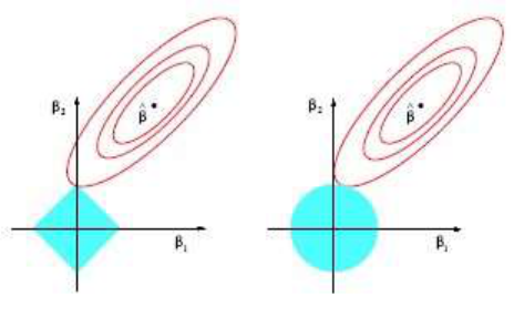
Figure 2.2, the ellipses correspond to the contours of the residual sum of squares (RSS): the inner
ellipse has smaller RSS, and RSS is minimized at ordinal least square (OLS) estimates. We are
trying to minimize the ellipse size and circle simultaneously in the ridge regression. The ridge
estimate is given by the point at which the ellipse and the circle touch.

10
Figure 2.2: Geometric Interpretation of Ridge Regression
Lasso Regression
Lasso (Least Absolute Shrinkage and Selection Operator) Regression is another variant of linear
regression that employs regularization to address the limitations of OLS. Like Ridge Regression,
Lasso adds a penalty term to the objective function. However, instead of using the sum of the
squared coefficients, Lasso uses the sum of the absolute values of the coefficients as the penalty
term ("STAT 508: Applied Data Mining and Statistical Learning."). Below you will see the
subtle but important change between Ridge and Lasso.
11
This difference in the penalty term leads to a unique property of Lasso Regression: it encourages
sparsity in the resulting model. When the regularization strength is sufficiently large, some of the
coefficients may be exactly zero, effectively excluding the corresponding features from the
model. This makes Lasso Regression particularly useful for feature selection in high-dimensional
data sets, as it can identify the most relevant features and discard the irrelevant ones.
However, Lasso Regression may struggle when there are highly correlated features, as it tends to
select only one of them, which could lead to suboptimal performance. Figure 2.3 shows how
Lasso (left) will compare to Ridge Regression (right). The lasso performs L1 shrinkage so that
there are "corners'' in the constraint, which in two dimensions corresponds to a diamond. If the
sum of squares "hits'' one of these corners, then the coefficient corresponding to the axis is
shrunk to zero.
Figure 2.3: Estimation picture of Lasso (left) and Ridge Regression (right)
Decision Tree
A Decision Tree is a non-parametric model that represents a series of decision rules based on the
values of input features ("Decision Tree and Random Forest Explained."). The tree is built by
12
recursively splitting the data into subsets according to the feature values. At each node of the
tree, a decision rule is applied based on the value of a specific feature. This rule is chosen to
maximize the purity of the resulting subsets, which is typically measured using criteria such as
Gini impurity or information gain. The process continues until a stopping criterion is reached,
such as a maximum tree depth or a minimum number of samples per leaf.
Decision Trees can be used for both classification and regression tasks. In classification tasks,
the majority class in each leaf node represents the predicted class for the samples reaching that
node. In regression tasks, the average value of the target variable in each leaf node is used as the
prediction for the samples reaching that node.
Decision Trees are intuitive and easy to interpret, as they resemble human decision-making
processes. They can handle both numerical and categorical features, and they do not require any
assumptions about the distribution of the data. However, Decision Trees can be prone to
overfitting, especially when they are deep, as they can become too specific to the training data.
This issue can be mitigated by pruning the tree or using ensemble methods, such as Random
Forests.
Random Forest
Random Forest is an ensemble learning method that combines multiple Decision Trees to
improve the overall performance and stability of the model. The idea behind Random Forest is
that by aggregating the predictions of multiple weak learners (individual Decision Trees), the
13
resulting model can achieve better generalization and robustness ("Decision Tree and Random
Forest Explained.").
To construct a Random Forest, multiple Decision Trees are trained on different subsets of the
training data, generated by bootstrapping (sampling with replacement). In addition, at each node
of the tree, a random subset of features is considered for splitting, which introduces more
diversity among the trees. Once all the trees are built, their predictions are combined by
averaging (in the case of regression) or by taking a majority vote (in the case of classification) to
obtain the final prediction of the Random Forest.
Random Forests are particularly effective in reducing overfitting and improving the stability of
the model, as they combine the predictions of multiple trees, each trained on a different subset of
the data and features. They can handle a wide range of data types and are robust to noise and
outliers. However, Random Forests can be computationally expensive, especially when the
number of trees and the depth of the trees are large, and they may not be as interpretable as
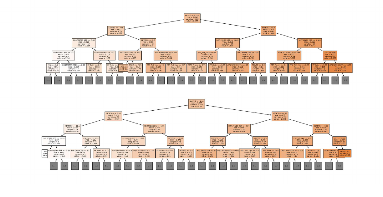
individual Decision Trees. Figure 2.4 demonstrates the first two decision trees in the Random
Forest model in our study.
14
Regularized Adjusted Plus Minus (RAPM)
Regularized Adjusted Plus-Minus (RAPM) is an advanced basketball statistic that aims to
measure a player's impact on their team's performance while accounting for the quality of
teammates and opponents on the court. RAPM builds upon the basic plus-minus statistic, which
calculates the point differential (points scored minus points allowed) while a player is on the
court ("Regularized Adjusted Plus-Minus (RAPM)."). However, plus-minus can be misleading
because it does not take into account the quality of a player's teammates or opponents, which can
significantly influence the point differential.
RAPM addresses these limitations by incorporating a Bayesian regularization technique. It uses
play-by-play data and lineup information to estimate the individual contributions of each player
Figure 2.4: Decision Tree’s 1 and 2 for the Random Forest model in this study
15
while controlling for the strength of their teammates and opponents. This is achieved by solving
a linear regression problem with a prior distribution on the player's impact, which helps to shrink
extreme estimates and reduce overfitting.
The RAPM value represents the estimated point differential per 100 possessions that a player
contributes to their team relative to an average player in the league. A positive RAPM indicates
that a player has a positive impact on their team's performance, while a negative RAPM suggests
a detrimental impact.
RAPM is considered an important statistic in basketball for several reasons:
Comprehensive Evaluation: RAPM accounts for both offensive and defensive contributions of
a player, providing a more comprehensive evaluation than traditional box score statistics like
points, rebounds, and assists.
Context Adjustment: By controlling for the quality of teammates and opponents, RAPM offers
a more accurate estimate of a player's individual impact on their team's performance,
independent of the surrounding context.
Predictive Power: RAPM has been shown to have strong predictive power for team success,
making it a valuable tool for player evaluation and roster construction.

16
Stability: The regularization technique used in RAPM helps to reduce noise and produce more
stable estimates across different seasons and lineups.
While RAPM is a powerful tool, there are some drawbacks to it.
This includes a high threshold of data requirements as it relies on
play-by-play data and lineup information that can be challenging
to obtain, especially historically. The quality of the analysis
depends on the accuracy and completeness of our data. It can also
be noisy especially when dealing with small sample sizes or
players who have limited playing time. This leads to a degree of
uncertainty in our results. Lastly, there is a lack of contextual
information in RAPM. It provides a single value that estimates a
player’s overall impact on team performance. It does not tell you
any insights into specific aspects of a player’s game, such as
shooting, rebounding, or playmaking. This makes it difficult to
identify areas for improvement or understand the underlying
factors driving a player's RAPM value.
Overall, RAPM is an essential tool for basketball analysts and decision-makers, as it provides a
more accurate and context-adjusted measure of a player's contributions to their team's success. In
Figure 2.5, a list of RAPM values for the top players is presented, encompassing the three year
period from 2020 to 2023.
Figure 2.5: 3-year RAPM (2020-
2023)
17
Chapter 3: Methodology
In this methodology chapter, we will delve into the details of the process and techniques
employed to build a statistical learning model for evaluating NBA players using player tracking
data. The chapter will be structured into several sections, each highlighting a crucial aspect of the
research methodology.
Firstly, we will begin with a thorough description of the dataset used in our study, including its
source, the number of seasons, players, and games covered. This section will also provide an
overview of the various variables present in the player tracking dataset and their respective
definitions to ensure a comprehensive understanding of the data.
Next, we will discuss the data preprocessing and cleaning procedures undertaken to ensure the
quality and reliability of the dataset. This includes handling missing values and outliers, as well
as any necessary data transformation.
The main focus of the chapter will be on the models employed in the study. We will outline the
feature engineering and selection process that enables us to extract relevant information from the
player tracking dataset. This will be followed by a description of the model training and
coefficient estimation techniques used to create our statistical models.
Subsequently, we will present the model evaluation criteria and validation techniques employed
in our study, such as cross-validation, to ensure the robustness and generalizability of our
findings. This section will also explore the analysis of models using all features and the analysis
of models using only the most important features, shedding light on the significance of feature
selection and the impact of dimensionality reduction on model performance.
18
By the end of this chapter, you will have a comprehensive understanding of the research
methodology used to build a statistical model for evaluating NBA players using player tracking
data. This will serve as a foundation for the subsequent chapters, where we will discuss the key
findings of our study, their implications for the world of professional basketball, and potential
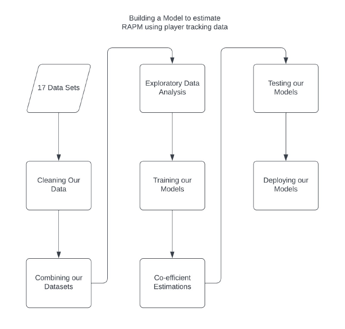
avenues for future research. In figure 3.1, a flowchart illustrating our methodology process is
displayed. The process begins with the initial data sets and concludes with the deployment of our
model.
Figure 3.1: Flowchart of our Methodology process
19
Dataset Description
The dataset used for this thesis is obtained from the NBA's publicly available player tracking
data, which includes information on player performance and movements during games ("NBA
Advanced Stats: Player Advanced Stats."). The dataset covers nine seasons (2013-2022) and
contains data for approximately 500 players per season. There are a total of 178 feature variables
in our dataset as well as our target variable RAPM in a separate dataset ("RAPM: Regularized
Adjusted Plus-Minus."). Below we list the 30 most important features in the dataset. To see all
the variables in our study and the definitions for each ("NBA.com/Stats Glossary."), please refer
to the appendix section.
PLUS-MINUS: A statistic that measures the point differential when a player is on the court,
comparing the team's performance with and without the player.
NET RATING: A metric that calculates the point differential per 100 possessions between a
team's offensive and defensive ratings.
LOSS: A game outcome in which a team scores fewer points than their opponent.
WIN: A game outcome in which a team scores more points than their opponent.
TOUCHES: The number of times a player touches the ball during a game.
PASSES RECEIVED: The number of passes a player receives from teammates during a game.
ASSIST RATIO: The percentage of a player's possessions that end with an assist.
TURNOVER: When a player loses possession of the ball to the opposing team.
20
TOV AT ELBOW: Turnovers that occur in the elbow area of the court, near the free-throw line.
CONTESTED REBOUNDS: A rebound in which a player secures the ball while being
challenged by an opponent.
PASSES MADE: The number of passes a player makes to teammates during a game.
3PM PULL-UPS: Three-point field goals made off a pull-up jump shot.
STEAL: A defensive play in which a player takes the ball from an opponent.
TOV PERCENTAGE ON DRIVES: The percentage of turnovers that occur during a player's
drive to the basket.
USAGE PERCENTAGE: An estimate of the percentage of team plays involving a particular
player while on the court.
PACE: A measure of the number of possessions a team uses per 48 minutes of play.
PERSONAL FOUL PERCENTAGE ON DRIVES: The percentage of personal fouls committed
by a player during their drives to the basket.
TURNOVER PERCENTAGE IN PAINT: The percentage of turnovers that occur within the
painted area near the basket.
PERSONAL FOULS: Fouls committed by a player, resulting in free throws for the opposing
team or a change in possession.
OFFENSIVE RATING: The number of points a team scores per 100 possessions.
21
FANTASY POINTS: A scoring system used in fantasy basketball to measure a player's overall
performance.
FREE THROW PERCENTAGE ON DRIVES: The percentage of free throws resulting from a
player's drives to the basket.
PASS PERCENTAGE IN PAINT: The percentage of passes that are completed within the
painted area near the basket.
GAMES PLAYED: The total number of games a player has participated in during a season or
career.
PASS PERCENTAGE ON POST-UPS: The percentage of passes completed during post-up
plays.
FREE THROW PERCENTAGE IN PAINT: The percentage of free throws made from fouls
committed within the painted area near the basket.
TRUE SHOOTING PERCENTAGE: A shooting efficiency statistic that accounts for field goals,
three-point field goals, and free throws.
EFFECTIVE FIELD GOAL PERCENTAGE ON PULL-UPS: The adjusted field goal
percentage that accounts for the additional value of three-point field goals made from pull-up
jump shots.
DISTANCE MILES DEFENSE: The total distance covered by a player on the defensive end of
the court during a game, measured in miles.
22
MINUTES PLAYED: The total amount of time a player spends on the court during a game,
measured in minutes.
Dataset cleaning
Before analyzing the dataset for our models, we undertook several preprocessing and cleaning
steps to ensure data quality. The data consisted of sixteen separate datasets per year, each
representing a different player tracking category, and an additional RAPM dataset. Initially, we
verified the uniqueness of each variable's title and removed any duplicates. Subsequently, we
combined the datasets into a master dataset for modeling purposes.
Next, we added the target variable, RAPM, to the master dataset. Due to discrepancies in player
names within the RAPM dataset, we manually corrected these inconsistencies to ensure proper
alignment. We then converted the categorical Team variable into a numerical format using one-
hot encoding, making it suitable for our models. Following these processes, our dataset was
prepared and ready for model implementation.
Upon examining our thoroughly cleaned dataset, we determined that utilizing the most recent
data would yield the most accurate models. Rather than developing models for each individual
year, we opted to train our model on data from the 2021 season, as it represented the latest
completed season. Once the 2022 season concluded, we then deployed our model and evaluated
its performance using the most current data available.
Distribution of RAPM and Correlation Matrix
In our study, we must first check that our target variable, RAPM, has a normal distribution. A
normal distribution is important in our target variable as it ensures that the underlying
23
assumptions of many statistical techniques are satisfied. A normal distribution will help in
achieving unbiased estimates, reduce the impact of extreme variables, and facilitate the
interpretation of our results. When the target variable is normally distributed, our models become
more reliable, and the conclusions we draw from them are more valid and generalizable.
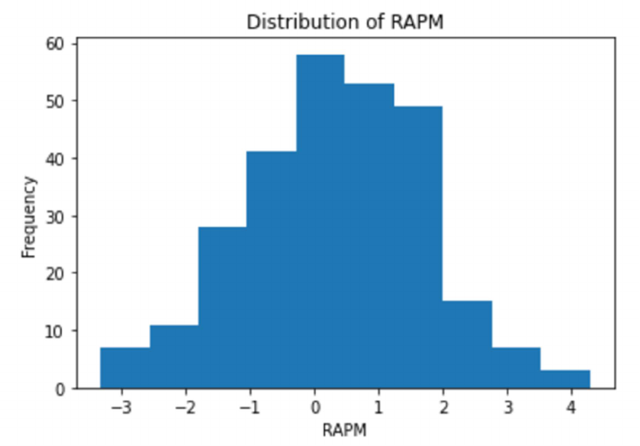
In Figure 3.2, we display the distribution of RAPM for our 2021 season. When looking at the
graph of the distribution of RAPM, we are looking for symmetry around the mean and a bell-
shaped curve. Since the graph shows a roughly equal number of observations on either side of
the mean and shows the characteristic pattern of the bell curve, we can conclude that the
distribution is normal. Inspection alone may not provide definitive evidence of a normal
distribution so we also do a Shapiro-Wilk test to confirm.
Figure 3.2: Distribution of RAPM (2021)
24
For our study, we conducted the Shapiro-Wilk test on the RAPM values and obtained a p-value
greater than 0.05. The Shapiro-Wilk statistic measures the deviation of the sample distribution
from a normal distribution. The test then calculates a p-value that indicates the probability of
obtaining the observed test statistic under the null hypothesis of normality. If the p-value is less
than the significance level (which is 0.05 in this case), we reject the null hypothesis and conclude
the data does not follow a normal distribution. In our case, the result is greater than 0.05 which
indicates that there is insufficient evidence to reject the null hypothesis, suggesting that the
RAPM values are likely to have originated from a normally distributed population.
Consequently, the assumption of normality for the RAPM values
in our dataset is considered reasonable, which is an important
prerequisite for the application of the chosen statistical models in
this thesis. By establishing the normality of the RAPM
distribution, we can proceed with confidence in our subsequent
analyses, knowing that our models' assumptions are met.
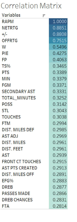
To aid in the process of coefficient estimation, we employ a
correlation matrix to examine the linear relationships between
features. The correlation matrix helps identify potential
multicollinearity among predictors, which can inform our feature
selection and the interpretation of the estimated coefficients.
Figure 3.3 displays the correlation matrix for RAPM related to all
other variables. It shows that net rating, plus/minus, and offensive
rating are all highly correlated with RAPM which makes sense as
Figure 3.3: Correlation Matrix (2021)
25
RAPM is a statistic that is derived from plus/minus similar to offensive rating and net rating.
Co-efficient Estimation of Our Models
In this study, we aim to estimate the coefficients for each of our selected features using five
different statistical models: Ordinary Least Squares (OLS), Ridge Regression, Lasso Regression,
Decision Tree, and Random Forest. Each model offers unique advantages in coefficient
estimation and allows for a comprehensive understanding of the relationships between the
features and our target variable, RAPM.
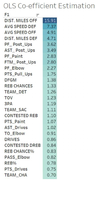
Ordinary Least Squares is the most straightforward linear regression model, which minimizes the
sum of squared residuals to obtain the best-fitting line. Figure 3.4 is our coefficient estimation
using Ordinary Least Squares.
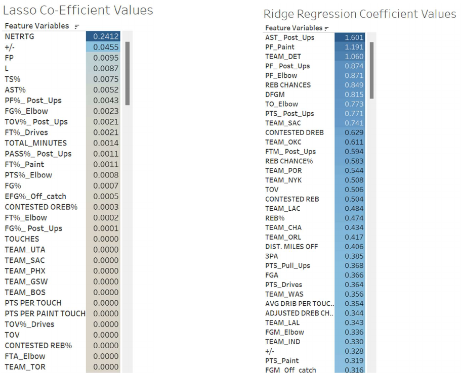
Ridge and Lasso Regression are extensions of OLS,
introducing regularization to prevent overfitting and improve
model generalization. Ridge Regression employs L2
regularization, while Lasso Regression uses L1 regularization,
which can also yield sparse models with some feature
coefficients set to zero. Figures 3.5 and 3.6 show the
coefficient values for Lasso and Ridge regression.
Figure 3.4: OLS Co-
efficient Estimation
(2021)
26
Figure 3.5: Lasso Co-efficient Estimation (2021) Figure 3.6: Ridge Co-efficient Estimation (2021)
Decision Trees and Random Forests are non-linear models capable of capturing complex
relationships in the data. Decision Trees recursively partition the data into subsets based on the
most significant features, while Random Forests aggregate the results of multiple Decision Trees
to reduce variance and improve predictive performance. Figures 3.7 and 3.8 reports the
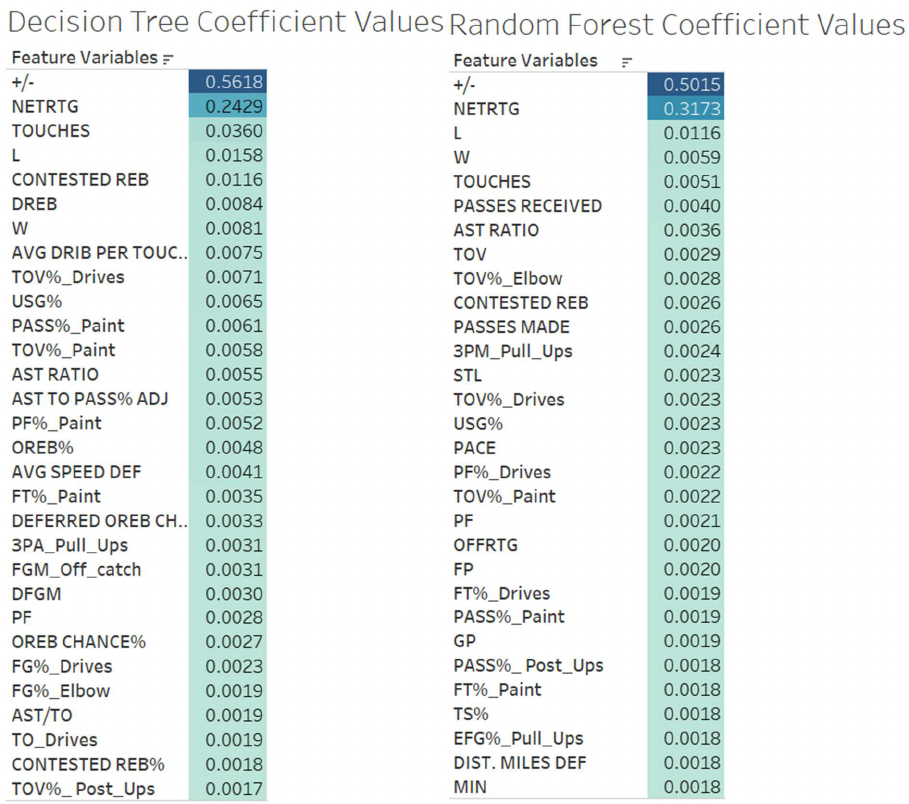
coefficients of our decision tree model and random forest model respectively.
27
Figure 3.7: Decision Tree Co-efficient Estimation (2021) Figure 3.8: Random Forest Co-efficient Estimation (2021)
By combining the insights from these five models and the correlation matrix, we can gain a
deeper understanding of the factors that contribute to the RAPM values and ultimately improve
our ability to evaluate NBA player performances.
28
Training our Models
In this section of the thesis, we will analyze the performance of our five selected statistical
models - Ordinary Least Squares (OLS), Ridge Regression, Lasso Regression, Decision Tree,
and Random Forest - with all the features included in the dataset. To ensure a robust evaluation
of the models, we split the data into training and testing sets using an 80% training and 20%
testing split. This approach allows us to train our models on a majority of the data while
reserving a portion for testing their performance and generalizability on unseen data.
The goal of this analysis is to understand the initial performance of each model in predicting
RAPM values and to identify any potential challenges, such as overfitting or multicollinearity,
that may arise from using the complete set of features. Following the analysis of the models with
all features, we will then focus on a more refined feature set by selecting the top 30 most
important features. The top 30 features are selected from the co-efficient estimation for each
individual model. For example, the top 30 features in the co-efficient estimation for OLS will
now be the only features used in our OLS model with optimized features. In our Random Forest
model with optimized features, we will use the top 30 features in our co-efficient estimation for
Random Forest. This selection is based on the feature importance rankings derived from our
initial models, and it aims to improve model interpretability, reduce overfitting, and potentially
enhance the predictive performance.
By comparing the results from both the full-feature and the reduced-feature analyses, we can
gain valuable insights into the robustness and efficiency of our statistical learning models in
evaluating NBA player performances using player tracking data.
29
To evaluate the performance of our models, we will employ three popular metrics: Mean
Squared Error (MSE), Root Mean Squared Error (RMSE), and R-squared. These metrics are
widely used in the field of regression analysis and can provide valuable insights into the
accuracy and goodness-of-fit of our models.
Mean Squared Error (MSE): MSE is the average of the squared differences between the
predicted and actual values. It measures the dispersion or spread of the errors, with larger values
indicating a greater difference between predictions and actual values. The primary advantage of
using MSE is that it penalizes larger errors more heavily than smaller errors, which is beneficial
in situations where large deviations from the true value are particularly undesirable.
Root Mean Squared Error (RMSE): RMSE is the square root of the MSE. It represents the
standard deviation of the residuals or prediction errors, which means it provides a measure of the
average distance between the predicted and actual values. Since RMSE is expressed in the same
unit as the target variable, it is easier to interpret compared to MSE. Lower values of RMSE
indicate better model performance, with a value of 0 representing a perfect fit.
R-squared: R-squared, also known as the coefficient of determination, measures the proportion
of the total variation in the target variable that is explained by the model. It ranges from 0 to 1,
with higher values indicating a better fit. An R-squared value of 1 indicates that the model
perfectly explains the variance in the target variable, while a value of 0 means that the model
does not explain any of the variance. R-squared is particularly useful for comparing the
performance of different models and assessing their ability to capture the underlying patterns in
the data.
30
These three metrics, when used in conjunction, provide a comprehensive assessment of our
models' performance. MSE and RMSE focus on the accuracy of the predictions, while R-squared
evaluates the overall goodness-of-fit. By considering all these metrics, we can ensure a balanced
evaluation of our models, taking into account both the magnitude of prediction errors and the
proportion of variance explained.
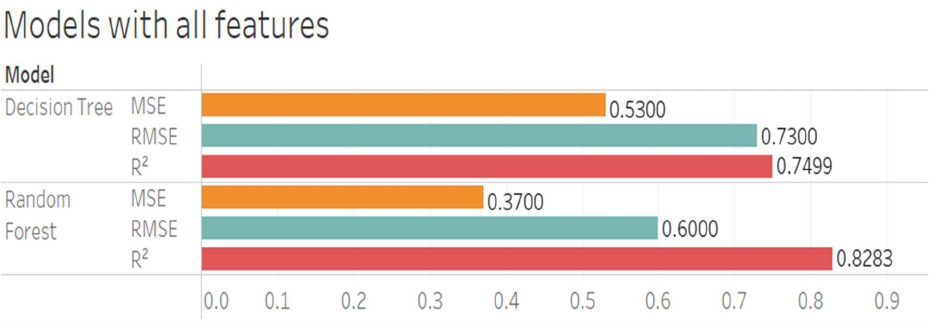
In Figures 3.9 and 3.10, you will see the results of our models against the testing data using the
three metrics discussed, MSE, RMSE, and R-squared (R
2
).
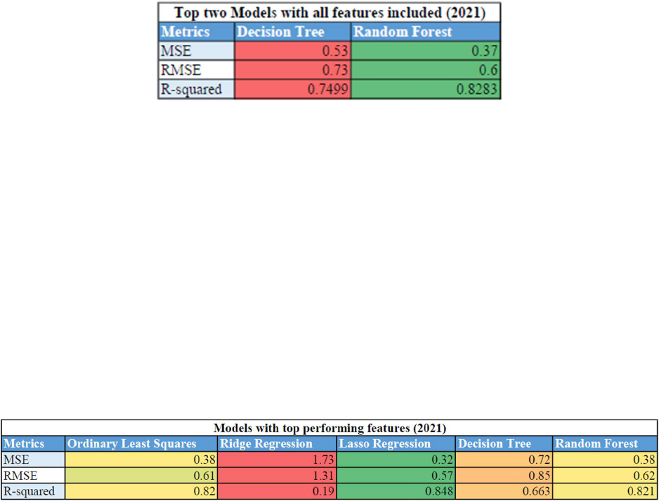
Figure 3.9: Top two models with all features included (2021)
31
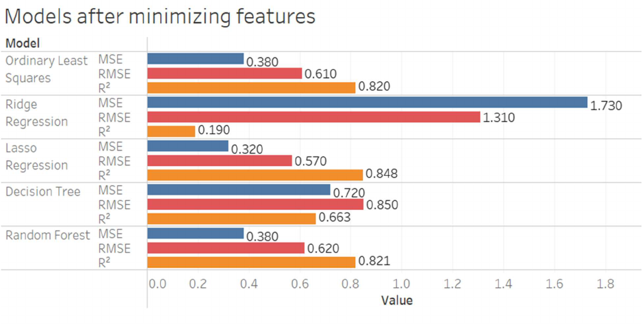
Figure 3.10: Statistical models with top performing features (2021)
Deployment of our Models
In the final step of our methodology, we aim to evaluate the performance of our models using
newly acquired 2022 data. This recently completed dataset provides an opportunity to test the
generalizability and predictive power of the models we have developed. By applying our trained
models to this independent dataset, we can gain insights into their real-world applicability and
robustness. This analysis will help us better understand the strengths and weaknesses of our
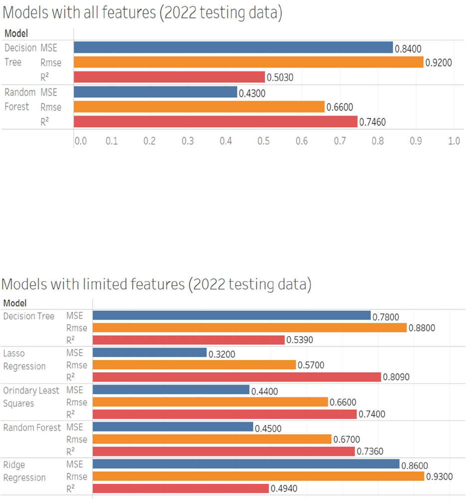
models and identify potential areas for improvement in future research. In figures 3.11 and 3.12,
you can see the results of our statistical learning models against the 2022 testing data.
32
Figure 3.11: Top two performing models with all features included against the 2022 testing data
Figure 3.12: Statistical models with top performing features against the 2022 testing data
In conclusion, the methodology chapter of this thesis has provided a detailed overview of the
dataset, variables of interest, data preprocessing and cleaning steps, and the modeling techniques
33
employed. We have described the comprehensive player tracking dataset, which contains
valuable information on various aspects of basketball performance, and discussed the target
variable RAPM, which is an important statistic in evaluating player contributions. Careful data
preprocessing and cleaning procedures were undertaken to ensure the highest possible data
quality and to prepare the dataset for use in our models.
The methodology also included a thorough explanation of the five regression models used in this
study: OLS, Ridge, Lasso, Decision Tree, and Random Forest. The feature engineering and
selection process, as well as model training and coefficient estimation methods, were discussed.
We have also outlined the model evaluation criteria and validation techniques, which involve
splitting the data into training and testing sets and using metrics such as MSE, RMSE, and R-
squared to assess the performance of each model.
Finally, we have described the process of analyzing the models using all features and using the
most important features, which allows for a comprehensive comparison of their performance in
both scenarios. By following this robust methodology, this study aims to provide valuable
insights into the relationships between player tracking data and player performance in basketball,
ultimately contributing to the field of sports analytics and enhancing our understanding of the
game.
34
Chapter 4: Analysis and Discussion
In this analysis section, we will dive into a comprehensive evaluation of the various models
developed in our study, focusing on their performance, interpretability, and practical implications
for NBA teams. We will start by comparing the performance of all models, considering both the
full feature and the top 30 feature scenarios. This comparison will allow us to identify the best-
performing model and further investigate its performance on the 2022 testing data.
Next, we will interpret the results of the chosen model and discuss its implications for basketball
analytics, player evaluation, and NBA team strategies. This section will provide valuable insights
into how our model can aid teams in making more informed decisions regarding player
development, roster construction, and game planning.
Finally, we will address the limitations of our study, considering factors such as data scope,
feature selection, model assumptions, and generalizability. This discussion will help to
contextualize our findings and highlight areas for future research and improvement in the field of
basketball analytics. By understanding the strengths and weaknesses of our approach, we can
better appreciate the potential impact of our work on the world of professional basketball.
Comparing our results
In this section, we analyze and discuss the performance of our models using the Mean Squared
Error (MSE), Root Mean Squared Error (RMSE), and R-squared metrics. The models are
compared in two scenarios: using all features and using only the top 30 most important features,
as identified by the coefficient analysis performed earlier in the study.
35
Initially, we focus on the results obtained using all features. The Random Forest model
outperforms the Decision Tree model, with lower MSE (0.37 vs. 0.53) and RMSE (0.60 vs. 0.73)
and a higher R-squared value (0.8283 vs. 0.7499). This is shown in Figure 4.1. This indicates
that the Random Forest model has better predictive accuracy and explains more variability in the
RAPM.
Figure 4.1: Table of top two performing model’s metrics
Next, we examine the results for models using only the top 30 features selected from the
coefficient analysis. The Lasso Regression model demonstrates the best performance with the
lowest MSE (0.32) and RMSE (0.57) and the highest R-squared value (0.848). Figure 4.2
displays this information. This result suggests that Lasso Regression provides a more accurate
and reliable prediction of RAPM when using a reduced set of features, which can lead to a more
interpretable and parsimonious model.
Figure 4.2: Table of model’s metrics with top performing features
Finally, we consider the model performance using the 2022 testing data. Among the models with
all features, Random Forest performs the best, with lower MSE (0.43 vs. 0.84) and RMSE (0.66
vs. 0.92) and a higher R-squared value (0.7460 vs. 0.503) than the Decision Tree model. Figure
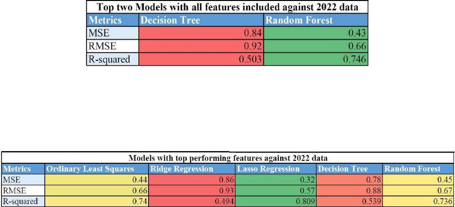
36
4.3 shows this information. In the case of models with only the top 30 features, Lasso Regression
outperforms the other models, exhibiting the lowest MSE (0.32) and RMSE (0.57) and the
highest R-squared value (0.8090). Figure 4.4 displays these results.
Figure 4.3: Table of top two performing models against 2022 data
Figure 4.4: Table of models metrics with top performing features against 2022 data
In summary, the Random Forest model performs the best when using all features, while Lasso
Regression demonstrates the best performance when using only the top 30 features. When
considering the 2022 testing data, Lasso Regression with the top 30 features shows the best
overall performance, indicating its effectiveness in predicting RAPM values. To further show
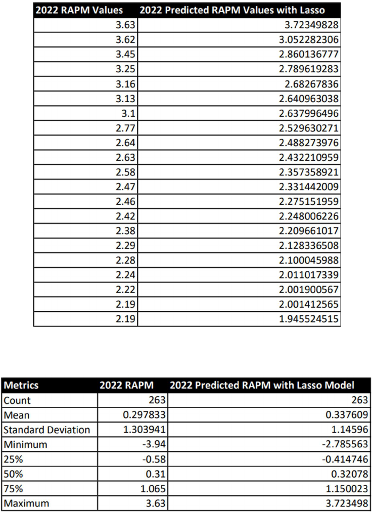
how well our Lasso Regression model predicts RAPM values, Figure 4.5 shows the top RAPM
values for 2022 next to our predicted values. Figure 4.6 shows the metrics of the 2022 RAPM
values and the metrics for our predicted values.
37
Figure 4.5: 2022 RAPM Values vs 2022 Predicted RAPM Values with Lasso
Figure 4.6: 2022 RAPM metrics vs 2022 Predicted RAPM with Lasso metrics
This model balances accuracy and simplicity, providing a reliable and interpretable solution for
future analysis and applications.
38
Implications for NBA teams
The best-performing model, Lasso Regression with the top 30 features, offers valuable insights
and applications for basketball analytics, NBA teams, and player evaluation. By leveraging this
model, various stakeholders can gain a deeper understanding of player performance, optimize
team strategies, and make more informed decisions regarding player acquisitions and
development. Here are some specific applications and benefits of utilizing this model in
basketball analytics:
Improved player evaluation: Using the Lasso Regression model, NBA teams can better assess
a player's overall performance by considering the most relevant features that contribute to their
RAPM. This holistic evaluation can help teams identify undervalued players or potential
weaknesses in their opponents' rosters.
Data-driven coaching and game strategies: The model can be used to identify patterns and
tendencies in player performance and provide recommendations for optimizing offensive and
defensive strategies. Coaches can use these insights to make adjustments during games or
develop targeted training programs that focus on specific skill sets.
Roster optimization: The model can help teams find the optimal mix of players that
complement each other, maximizing their combined RAPM. This can lead to improved on-court
chemistry and overall team success.
Player development: By identifying the most important features contributing to RAPM, the
model can help teams design individualized development programs for their players. This can
enhance player growth, improve their RAPM, and ultimately contribute to team success.
39
Salary cap management: Using the insights from the Lasso Regression model, NBA teams can
make more informed decisions about player contracts, ensuring that they allocate resources
efficiently and stay within the salary cap while maximizing team performance.
Draft and trade analysis: The model can be used to evaluate potential draft prospects and trade
targets, enabling teams to make more informed decisions when acquiring new players. This can
help teams build a stronger roster and improve their chances of success in the long run.
Limitations of our study
While our study provides valuable insights into predicting player performance using advanced
basketball metrics, there are several limitations to consider:
Limited data scope: Our study is based on data from specific seasons up until 2022, which may
not capture the full spectrum of player performance or game contexts. Additionally, there may be
changes in the game, player performance trends, or team strategies that our model does not
account for.
Feature selection: Although we used the top 30 features based on our coefficient analysis, there
may be other important features that were not considered, or the selected features may not be the
most optimal for predicting RAPM across all scenarios.
Model assumptions: The study relies on several model assumptions, such as normal distribution
of RAPM and the use of linear regression techniques. These assumptions may not hold true in all
cases, potentially affecting the model's performance.
40
Generalizability: Our models were trained and tested on specific data sets, and their
performance on new data or different leagues may be different. The models might need to be
retrained or adapted for different contexts to ensure their reliability.
Overfitting: Although we have attempted to minimize overfitting by using regularization
techniques like Lasso and Ridge Regression, there is still a possibility that the model could be
overfitting to the training data, leading to reduced performance on new data.
Model interpretability: While Lasso Regression was our best-performing model, it can be more
challenging to interpret compared to simpler models like OLS. This may make it harder for
stakeholders to understand and trust the predictions made by the model.
Addressing these limitations in future research can help improve the accuracy and reliability of
our models and expand their applicability to other basketball analytics tasks. This may involve
incorporating additional data sources, exploring alternative feature selection methods, or
experimenting with different modeling techniques.
In conclusion, the Lasso Regression model with the top 30 features can significantly enhance
basketball analytics, providing NBA teams with valuable insights and tools for player evaluation,
coaching strategies, roster optimization, and more. By leveraging this model, teams can make
more informed decisions and ultimately improve their performance on the court.
Our analysis has provided a thorough examination of the various models used to predict player
performance in the context of NBA basketball. By comparing these models, we have identified
the best-performing one, which has significant implications for basketball analytics, player
evaluation, and team decision-making. The insights gained from our model can help NBA teams
41
make more informed decisions, ultimately leading to better on-court performance and increased
competitiveness.
Furthermore, our study has revealed the importance of feature selection in model development,
as evidenced by the improved performance of the models using the top 30 features. This finding
highlights the need for careful consideration of the features included in any predictive model, as
well as the value of a comprehensive coefficient analysis.
While our study has provided valuable insights, we have also acknowledged its limitations,
paving the way for future research to build upon our findings and refine the methods used in
basketball analytics. As the field of sports analytics continues to grow, we can expect more
sophisticated models and techniques to emerge, driving the evolution of basketball analytics and
further enhancing our understanding of player performance in the NBA.
42
Chapter 5: Conclusions
This thesis, titled "Building a Statistical Model for Evaluation of NBA Players Using Player
Tracking Data," aimed to find faster and more accurate ways to measure NBA player
performances. Our research question sought to determine if publicly available player tracking
data could improve existing measures for evaluating player performances. The study acquired
player tracking data from the 2013 to 2021 seasons and used RAPM as the target variable due to
its effectiveness in ranking player value over the long term.
Five statistical learning models, including Ordinary Least Squares, Ridge regression, Lasso
regression, Decision Tree, and Random Forest, were employed to estimate RAPM using player
tracking data as features. The models were also tested using only the top 30 most important
features ranked by their coefficients. The models' performance was further assessed using newly
acquired 2022 player tracking data. Key findings revealed that Lasso regression and Random
Forest performed the best among all models at predicting RAPM values.
The implications of these findings suggest that by using player tracking statistics that settle
earlier, we can achieve a more accurate estimate of future RAPM. Consequently, teams can gain
an advantage in player evaluations, enabling them to acquire the best-performing players before
other teams become aware of their potential.
However, it is essential to acknowledge the limitations of this study, such as the reliance on
available player tracking data and potential biases in the RAPM metric. Despite these limitations,
the contributions of this thesis have the potential to impact the way NBA teams approach player
evaluation and strategy in the future.
43
Future studies and research in this topic hold great potential to build on our study and continue
the work in understanding basketball. As the accuracy and availability of player tracking data
continues to improve, researchers can develop even more sophisticated models for evaluating
player performances and predicting outcomes. Integrating advanced machine learning techniques
and exploring novel features could lead to a deeper understanding of the game, uncovering
hidden patterns and previously unknown relationships among player statistics. Furthermore, real-
time analysis and predictive models could be incorporated into coaching strategies, allowing
teams to make data-driven adjustments during games. Additionally, future research could
explore ways to refine player evaluation metrics, reducing biases and better accounting for
intangibles, such as leadership and teamwork. Ultimately, the continued evolution of NBA
analytics has the potential to revolutionize not only player evaluation and team strategy but also
enhance the overall understanding and appreciation of the game of basketball.
In conclusion, this study demonstrated that combining statistical models with player tracking
data enables us to estimate end-of-season statistics earlier. The ability to make accurate early
estimates of player performance empowers teams to make informed decisions in acquiring top
talent, ultimately leading to a more competitive and exciting NBA landscape.

44
Chapter 6: References
"History of Basketball Leagues." All About Basketball,
https://www.allaboutbasketball.us/basketball-history/history-of-basketball-leagues.html.
Accessed 1 May 2023.
"NBA Advanced Stats: Player Advanced Stats." NBA.com, NBA Media Ventures, LLC,
https://www.nba.com/stats/players/advanced. Accessed 1 May 2023.
"NBA Analytics Movement: How Basketball Data Science Has Changed the Game."
NBAstuffer, https://www.nbastuffer.com/analytics101/nba-analytics-movement/. Accessed 1
May 2023.
"NBA.com/Stats Glossary." NBA.com, National Basketball Association. Accessed 4 May 2023.
https://www.nba.com/stats/help/glossary.
"RAPM: Regularized Adjusted Plus-Minus." NBA Shot Charts,
http://nbashotcharts.com/rapm?id=548833052. Accessed 1 May 2023.
"Regularized Adjusted Plus-Minus (RAPM)." NBAstuffer, NBAstuffer.com. Accessed 4 May
2023. https://www.nbastuffer.com/analytics101/regularized-adjusted-plus-minus-rapm/.

45
"STAT 508: Applied Data Mining and Statistical Learning." Penn State Eberly College of
Science, Pennsylvania State University, https://online.stat.psu.edu/stat508/. Accessed 1 May
2023.
"Where Basketball Was Invented: The Birthplace of Basketball." Springfield College,
https://springfield.edu/where-basketball-was-invented-the-birthplace-of-
basketball#:~:text=The%20Birthplace%20of%20Basketball,know%20it%20to%20be%20today.
Accessed 1 May 2023.
Gulve, Aishwarya. "Ordinary Least Square (OLS) Method for Linear Regression." Analytics
Vidhya, Medium, 9 July 2020, https://medium.com/analytics-vidhya/ordinary-least-square-ols-
method-for-linear-regression-ef8ca10aadfc. Accessed 1 May 2023.
Mays, Robert. "How Basketball-Reference Got Every Box Score." Grantland, ESPN Internet
Ventures, 30 Jan. 2012. https://grantland.com/the-triangle/how-basketball-reference-got-every-
box-score/.
Yildirim, Soner. "Decision Tree and Random Forest Explained." Towards Data Science,
Medium, 11 Feb, 2020. https://towardsdatascience.com/decision-tree-and-random-forest-
explained-8d20ddabc9dd.
Zimmerman, Kevin. "The NBA releases SportVU Camera Statistics." SB Nation, Vox Media, 1
Nov. 2013. https://www.sbnation.com/nba/2013/11/1/5055376/nba-sportvu-camera-statistics.
46
Appendix
Definitions of our 178 feature Variables
TEAM: The NBA team the player belongs to.
AGE: The age of the player.
GAMES PLAYED: The total number of games the player participated in during a season.
WIN: The total number of games the player's team won during a season.
LOSS: The total number of games the player's team lost during a season.
MINUTES PLAYED: The total number of minutes the player was on the court during a season.
OFFENSIVE RATING: A metric that estimates the number of points a player contributes per
100 possessions while on the court.
DEFENSIVE RATING: A metric that estimates the number of points a player allows per 100
possessions while on the court.
NET RATING: The difference between a player's offensive and defensive rating.
ASSIST PERCENTAGE: The percentage of teammate field goals a player assisted on while on
the court.
TURNOVER RATIO: The number of turnovers a player commits per 100 possessions while on
the court.
47
EFFECTIVE FIELD GOAL PERCENTAGE: A statistic that adjusts for the fact that three-point
field goals are worth more than two-point field goals.
TRUE SHOOTING PERCENTAGE: A measure of shooting efficiency that takes into account
field goals, three-point field goals, and free throws.
USAGE PERCENTAGE: The percentage of team plays used by a player while they were on the
floor.
PACE: The number of possessions a team uses per 48 minutes.
PLAYER IMPACT ESTIMATE: A metric that measures a player's overall impact on the game,
expressed as a percentage.
POINTS OFF CATCH AND SHOOT: The number of points a player scores as a result of
catching a pass and shooting without dribbling.
DRIVES: The number of times a player drives to the basket.
ELBOW TOUCHES: The number of times a player touches the ball at the elbow area of the
court.
CONTESTED REBOUNDS: The number of rebounds a player grabs when an opposing player is
also attempting to grab the rebound.
PAINT TOUCHES: The number of times a player touches the ball in the paint area of the court.
POST UPS: The number of times a player receives the ball in the post area of the court.
48
POINTS OFF PULL UP: The number of points a player scores as a result of dribbling and
shooting without passing.
TOUCHES: The total number of times a player touches the ball during a game.
DISTANCE FEET: The total distance a player covers during a game, measured in feet.
AVERAGE SPEED: The average speed at which a player moves during a game, measured in
miles per hour.
POINTS: The total number of points a player scores during a game.
REBOUNDS: The total number of times a player retrieves the ball after a missed field goal or
free throw.
ASSISTS: The total number of passes a player makes that lead directly to a made field goal by a
teammate.
TURNOVERS: The total number of times a player loses possession of the ball to the opposing
team.
STEALS: The total number of times a player takes the ball away from an opposing player.
BLOCKS: The total number of times a player deflects an opposing player's field goal attempt.
PERSONAL FOULS: The total number of Illegal physical contact violations, leading to free
throws or possession for the opposing team.
49
DOUBLE DOUBLES: The total number of games in which a player records double-digit values
in two of the five major statistical categories (points, rebounds, assists, steals, and blocks) during
a single game.
TRIPLE DOUBLES: The total number of games in which a player records double-digit values in
three of the five major statistical categories (points, rebounds, assists, steals, and blocks) during a
single game.
PLUS/MINUS: A statistic that measures the point differential when a player is on the court, i.e.,
the difference between the points scored by the player's team and the points scored by the
opposing team while the player is on the court.
TOTAL MINUTES PLAYED: The sum of all minutes played by a player throughout the entire
season.
Many of the variables in the list below are repeated for different contexts or situations (e.g., for
catch and shoot, pull-up, elbow touches, post-ups, and paint touches). Provided are general
definitions for these variables, which can be applied to their specific contexts.
A. FIELD GOALS MADE: The total number of successful shots from the field in the specified
context.
B. FIELD GOALS ATTEMPTED: The total number of shots attempted from the field in the
specified context.
C. FIELD GOAL PERCENTAGE: The ratio of successful field goals to field goal attempts in
the specified context.
50
D. FREE THROWS MADE: The total number of successful free throws in the specified context.
E. FREE THROWS ATTEMPTED: The total number of free throw attempts in the specified
context.
F. FREE THROW PERCENTAGE: The ratio of successful free throws to free throw attempts in
the specified context.
G. POINTS: The total number of points scored in the specified context.
H. POINTS PERCENTAGE: The percentage of a player's total points that come from the
specified context.
I. PASSES: The total number of passes made in the specified context.
J. PASS PERCENTAGE: The percentage of a player's total passes that come from the specified
context.
K. ASSISTS: The total number of assists made in the specified context.
L. ASSIST PERCENTAGE: The percentage of a player's total assists that come from the
specified context.
M. TURNOVERS: The total number of turnovers committed in the specified context.
N. TURNOVER PERCENTAGE: The percentage of a player's total turnovers that come from
the specified context.
O. PERSONAL FOULS: The total number of personal fouls committed in the specified context.
51
P. PERCENTAGE OF TEAM'S PERSONAL FOULS: The percentage of a player's personal
fouls relative to the total number of personal fouls committed by the team in the specified
context.
For variables related to rebounding, defensive plays, and other statistics with similar groupings,
the general definitions provided above can be applied to the specific context or situation
mentioned in the variable name.
