L62 CTE - BE LPL.vp

Spreadsheets: Formatting

Unit: Technology

Problem Area: Create Spreadsheets

Lesson: Spreadsheets: Formatting

Student Learning Objectives.

Instruction in this lesson should result in students

achieving the following objectives:

Describe spreadsheets.

Describe basic spreadsheet components.

Format a spreadsheet.

Use spreadsheet formulas and functions.

¢ Resources.

The following resources may be useful in teaching this lesson:

E-unit(s) corresponding to this lesson plan. CAERT, Inc. http://www.mycaert.com.

Brown, Liza. “20 Tips That Can Make Anyone An Excel Expert,” Lifehack. Accessed Apr. 22,

2019. https://www.lifehack.org/articles/technology/20-excel-spreadsheet-secrets-youll-

never-know-you-don’t-read-this.html.

Nicol, Will. “Master The Way Of The Spreadsheet With These Excel Tips And Tricks,” Digital

Trends. Accessed Apr. 22, 2018. https://www.digitaltrends.com/computing/microsoft-

excel-tips-and-tricks/.

Smith, Sue. “How Do Companies Use Spreadsheets?” Chron. Accessed Apr. 22, 2019.

http://smallbusiness.chron.com/companies-use-spreadsheets-54058.html

Zao-Sanders, Marc. “The 10 Most Useful Things You Can Do In Excel,” BusinessInsider.

Accessed Apr. 22, 2019. http://www.businessinsider.com/excel-tips-and-tricks-2017-

11.

Lesson: Spreadsheets: Formatting

Page 1 u www.MyCAERT.com

Equipment, Tools, Supplies, and Facilities

Overhead or PowerPoint projector

Visual(s) from accompanying master(s)

Copies of sample test, lab sheet(s), and/or other items designed for duplication

Materials listed on duplicated items

Computers with printers and Internet access

Classroom resource and reference materials

Key Terms.

The following terms are presented in this lesson (shown in bold italics):

Interest Approach.

Use an interest approach that will prepare the students for the

lesson. Teachers often develop approaches for their unique class and student situations. A

possible approach is included here.

Ask your students: “How many of you have used spreadsheets for schoolwork?

What businesses often use spreadsheets?” In small groups, discuss possible

uses for spreadsheets by the following professionals: accounting, construction

contractor, healthcare administrator, restaurant manager, and retail sales

manager. Use VM–A to review businesses and industries that use spreadsheets.

Virtually all professions use spreadsheets for some aspect of their operations.

Spreadsheets are good for personal use also.

Lesson: Spreadsheets: Formatting

Page 2 u www.MyCAERT.com

absolute cell

reference

arguments

arithmetic operators

auto format

AVERAGE

bar graph

cell

cell alignment

cell border

cell reference

circular reference

column

comparison operators

data

data displays

data table

fill handle

financial ratios

font

formatting

formula

formula bar

function

horizontal analysis

keyboard shortcut

label

line graph

MAX

MIN

model

operators

order of operations

page setup

pie chart

range

reference operators

ROUND

row

sheet

sheet tab

spreadsheet

SUM

syntax

trend analysis

value

workbook

worksheet

CONTENT SUMMARY AND

TEACHING STRATEGIES

Objective 1: Describe spreadsheets.

Anticipated Problem: What is a spreadsheet? What are the purposes of spreadsheets?

I. Spreadsheets

A spreadsheet is a software application program that calculates, manages, and

stores data in rows and columns. It is the computer version of a paper-based

accounting worksheet. The uniqueness of a spreadsheet is the ability to calculate

values using mathematical formulas and the data in cells.

A. Excel, part of the Microsoft Office Suite, is the spreadsheet component of the

Microsoft Office Suite. Excel’s closest competitor is Google Sheets. Google Sheets

is a part of G Suite. Free spreadsheet applications, including OpenOffice and

LibreOffice, are available. Regardless of the brand, all spreadsheet programs

present tables of values, arranged in rows and columns, that can be manipulated

mathematically using both basic and complex arithmetic operations and functions.

B. The primary purpose of a spreadsheet is to store data in a structured, organized

format. Spreadsheets are used in a variety of ways, depending on the needs of

the business, industry, or individual.

1. Spreadsheets organize, store, and link related information.

2. Spreadsheets allow users to sort data alphabetically, numerically, or chrono-

logically.

3. Spreadsheets perform calculations on data using formulas.

4. Spreadsheets automatically recalculate answers when data components are

changed in them. Whenever data is updated inside the spreadsheet, all related

data calculations automatically update.

5. Spreadsheets show different scenarios for businesses and aid in decision-mak

ing. For example, a model is a spreadsheet containing data related to a spe

cific situation. A model can be used to answer the question, “What if...?”

Examples of common types of hypothetical questions are:

a. What if employees receive a 5% commission versus a 7% commission?

b. What if the cost of baking ingredients increases or decreases?

c. What if a student gets a score of 100 on a test compared to getting a

score of 83?

C. Data is often collected and held in spreadsheets before it is converted to a

display. Data displays are computer-generated charts, tables, and graphs, that

are used to show combinations of facts, numbers, words, observations, or

Lesson: Spreadsheets: Formatting

Page 3 u www.MyCAERT.com

descriptions. Data displays summarize information and present it in a visually

pleasing way. The most commonly used data display forms are:

1. A pie chart is a circular graphic divided into sectors that represent a propor

tion of the whole. Information related to budgets may be presented through a

chart that displays the percentage components of various budget line items. A

pie chart can show the breakdown of budgetary expenses.

2. A bar graph is a display of data using horizontal or vertical rectangular bars.

Bar graphs are often used to display budget changes, or variances from one

accounting period to another.

3. Horizontal analysis is a data display that compares financial information over

a series of historical periods. Horizontal analysis of the income statement usu

ally involves comparing two years’ income statements side-by-side with a third

column to report the variance between the two years. For example:

a. If sales are reported for the year ended December 31, 2018 as $50,000

and sales are reported for the year ended December 31, 2019 as

$45,000, then a positive variance of $5,000 would be reported.

Statement users would note that sales had increased by 11% ((50,000 –

45,000) ÷ 5000). The same process would be completed for each line

item of the income statement.

b. Horizontal analysis of the balance sheet is performed in the same manner

as for the income statement. Two years’ balance sheets are presented

side-by-side with a third column to report the variance. Accountants may

use bar graphs or data tables to present horizontal analysis in

presentations. A data table is a display of information using rows and

columns.

4. Trend analysis is a technical analysis that compares business data over a

certain time period, in order to identify trends. Trend lines may be drawn for

key items in the financial statements over several accounting periods. Trend

lines are frequently drawn for revenues, expenses, net income, and debt. Line

graphs may be used to display trend analysis in presentations. A line graph is

a display of information using a series of data points (or markers) connected

by straight-line segments to display changes in values.

5. Financial ratios are relationships/computations, based on a company’s finan

cial information, that are used for comparison purposes. Ratios are propor

tional, which allows small and large businesses to compare financial informa

tion. Financial ratios may be displayed as pie charts or bar graphs, depending

on the comparison being made.

Teaching Strategy:

Many techniques can be used to help students master this

objective. Use VM–A during the Interest Approach to generate a discussion about the

various ways spreadsheets might be used in different professions.

Lesson: Spreadsheets: Formatting

Page 4 u www.MyCAERT.com

Objective 2: Describe basic spreadsheet components.

Anticipated Problem: What are key spreadsheet components?

II. Spreadsheet components

A workbook is an electronic spreadsheet file. A worksheet (sheet) is an individual

spreadsheet within a larger workbook (of multiple worksheets) used to organize, store,

and link related information. A sheet tab is used to display the worksheet a user is

editing. The tabs appear below the worksheet grid area and allow a user to switch

from one worksheet to another in a workbook.

A. Data is factual information, collected together for analysis and use. Data is any

set of characters that can be stored in the cells of a spreadsheet. Spreadsheet

character types include values (numbers), labels, formulas, symbols, sound,

pictures, functions, etc. A value is numeric data entered into a cell.

B. A row is data that is stored in a series of cells, laid out horizontally in a

spreadsheet. Rows are designated by a number.

C. A column is data that is stored in a series of cells, laid out vertically in a

spreadsheet. Columns define the data contained in a table. Columns are identified

by a letter.

D. A cell is the most basic storage unit of data in a spreadsheet program, located at

the intersection of a column and a row. A cell is a box where data is entered and

stored. A cell reference is the column letter and row number used to identify a

specific cell (i.e., B3). A range is a group of cells selected in a spreadsheet row or

column. For example, in the formula “=sum(D1:D8)” the cells in column D1

through D8 are the range of cells that are added together.

E. A label is text that is typed into the cells of a spreadsheet, usually describing data

in the rows and columns surrounding it. Labels have no numeric value and cannot

be used in a formula or a function.

F. The formula bar is the spreadsheet location that shows the contents of the

current cell and allows the user to create and view formulas. The formula bar

appears directly above the column headings of a spreadsheet and displays the

information typed into the active cell. For example, if a cell that contains the

formula is clicked, such as “=A9+B3,” the cell shows the result of the formula.

However, the formula bar continues to display what was actually typed into the

cell which, in this case, is “=A9+B3.”

Teaching Strategy:

Many techniques can be used to help students master this

objective. Use VM–B to review the main components of a spreadsheet. Assign LS–A to

give students an opportunity to review the main features of spreadsheets found in Excel

and Google Sheets.

Lesson: Spreadsheets: Formatting

Page 5 u www.MyCAERT.com

Objective 3: Format a spreadsheet.

Anticipated Problem: What is formatting? What are spreadsheet format features and

options?

III. Formatting spreadsheets

Formatting is the arrangement of characteristics, such as fonts, numbers, cell

borders, etc., found in spreadsheets. To prevent changes to formatting, Excel allows

the user to apply a “lock” to prevent further editing.

A. Consistency is important in producing a professional document. Auto format is a

software feature that automatically changes the formatting or appearance of text.

It also allows several choices in creating enhancements. In Excel, format painter is

a feature that copies formatting from one place to another, and enhances the

consistency of the spreadsheet. To eliminate either feature, a user can “remove

formatting.”

B. Page setup is the term that describes the parameters set by the user to

determine how a spreadsheet appears when printed. A user can set the margin

width, the page orientation (portrait or landscape), and insert a header or a footer.

C. A user can format the cell alignment and utilize cell features to change the

appearance of the spreadsheet.

1. Cell alignment is the feature that describes how text or numbers are arranged

in a cell. Left-aligned characters begin on the left edge of the cell. Right-

aligned characters sit on the right edge of the cell. Justified characters are

equally spaced across a cell. Centered characters are placed equal distance

from the cell edge. Cell content can be indented (or tab-aligned).

2. A user can use the rotate feature (located in the format menu) to select and

reorient an object (images, text, etc.). The wrap text feature allows the entry

of more than one line of text or numbers in a cell. By using merge cells fea

ture, selected cells can be allowed to lengthen without changing column width.

In Excel, a user can merge two cells using a formula. Best fit allows the cre

ation of a column wide enough to show all the information. Row height

changes the standard row height to accommodate larger font sizes. Column

width changes the width of an entire column to view all cell content. An indi

cation that the column width must be changed is the “#####” display.

Shrink to fit allows cell content to fit in the cell without changing the cell size.

D. Font and style formatting address the appearance of the spreadsheet and can

enhance its functionality.

1. A font is the typeface used to create the spreadsheet. The font size is the

dimension of the font usually measured in “points.” For example, 72 points

equals an inch. Points dictate the height and dimension of the letters. Font

color can also be changed.

2. The style in which the text or numbers appear enhances the spreadsheet. Bold

makes text and numbers appear darker and heavier. Underline creates a line

Lesson: Spreadsheets: Formatting

Page 6 u www.MyCAERT.com

beneath the selected text or font to draw attention to the information. Italic

slants the text or numbers to the right. Any of the above can be used in combi

nation.

3. In Microsoft Excel, Borders is a built-in tool to access predefined border styles

built on Excel’s grid system. A cell border is a frame that can be placed

around the cell that includes options to enhance the line style and the color.

For example, cell shading (addition of color and/or pattern) can be applied in

any color or percent of color. If the finished appearance of the cell border and

shading is no longer desired, it is easy to alter or remove a formatting choice.

E. Number formatting makes the spreadsheet easier to read. Currency formatting

displays numbers as monetary values, such as a dollar sign ($), a pound sign (£),

etc. A user can apply percentage formatting to a cell that already contains a

number. Percentage formatting tells Excel to multiply a specific number by 100

and add the % sign. Large numbers are often easier to read if a comma is used as

a separator. To increase or decrease decimal places, a user can apply the

decrease or increase option.

Teaching Strategy:

Many techniques can be used to help students master this

objective. Use VM–C to review formulas and cell references.

Objective 4: Use spreadsheet formulas and functions.

Anticipated Problem: What is a formula? How are operators used in a formula? What is

a function?

IV. Formulas and functions

Formulas are an expression that tells the computer what math operation to perform

on a specific value. In other words, a formula conducts a calculation. Spreadsheet

formulas are often used to automatically perform operations and tasks. Spreadsheet

functions (preprogramed formulas) automatically perform common calculations.

Functions make a formula shorter and reduce the possibility of errors.

A. A formula is an expression that tells the computer what math operation to

perform on a specific value. The formula conducts a calculation. A formula must

always begin with an equal sign and use cell references as much as possible. For

example, =C5 + D7 + E8 is a formula that adds the numbers entered in cells

C5, D7, and E8.

1. Formulas are used to make business operations more accurate and efficient.

a. In order to recreate the same formula and perform the same operations

over several sets of data, formulas may be copied and pasted to different

cells, and even to different worksheets.

b. Formulas used in spreadsheets will recalculate answers automatically, as

the data entered in linked cells changes. Any time data is corrected or

updated, the related cells holding formulas also update their calculations.

Lesson: Spreadsheets: Formatting

Page 7 u www.MyCAERT.com

c. Hypothetical scenarios may be examined for decision-making based on

quick changes to data and the corresponding calculation changes.

d. When recalculations are necessary, spreadsheet formulas help eliminate

common mistakes caused by human error.

2. Operators are symbols used in a formula that indicate a specific type of cal

culation. There are four categories of operators.

a. Arithmetic operators perform basic mathematical operations, such as

addition, subtraction, multiplication, or division. The Excel arithmetic

operators are:

(1) + (plus sign) is the addition operator.

(2) – (minus sign) is the subtraction operator.

(3) * (asterisk) is the multiplication operator.

(4) / (forward slash) is the division operator.

(5) % is the percent operator.

(6) ^ (caret) is the exponentiation operator.

b. Comparison operators are operators that allow the user to compare two

values. Comparison operators are:

(1) > (greater than)

(2) < (less than)

(3) = (equal to)

c. The ampersand (&) is the text concatenation operator. It is used to join one

or more text strings to produce a single piece of text.

d. Reference operators are operators that combine cell ranges for

calculations. Reference operators are the colon, the comma, and the

space. The colon, “:” is the range operator. It produces one reference to all

the cells between two references. For example, A5:A15 references all cells

in the range including A5 through A15. The comma, “,” is the union

operator, which combines multiple references into one reference. A space

is the intersection operator. It produces one reference to cells common to

the two references.

3. Order of operations is the sequence of calculations in a formula. The com

puter software determines which calculation is first, which is second, etc.

a. The order of evaluation is: exponents, multiplication/division, and addition/

subtraction.

b. Operators of equal priority are evaluated left to right.

c. Parentheses change the priority order. Calculations within parentheses are

performed first.

d. Excel follows general mathematics rules for calculations:

(1) Parentheses

(2) Exponents

(3) Multiplication and division

(4) Addition and subtraction.

Lesson: Spreadsheets: Formatting

Page 8 u www.MyCAERT.com

[NOTE: Use the acronym PEMDAS (Please Excuse My Dear Aunt Sally) to

remember the order of operations.]

4. Always use the most efficient form of a formula. Frequently, there is more than

one way to perform a calculation. For example, when calculating an average,

the user could enter =(D4 + D5 + D6 + D7)/4. However, using the AVERAGE

function command would be more efficient. In this case, the user would simply

enter =AVERAGE(D4:D7) or =AVERAGE (D4, D5, D6, D7).

5. Excel displays an error message for an invalid formula when a mistake has

been made setting up the formula. Common errors include:

a. Dividing by 0

b. Unequal number of parentheses

c. Misplaced operators or commas

d. Circular reference (A circular reference is a formula in a cell that directly

or indirectly refers to its own cell.)

6. When the same basic formula is needed, users can copy that formula instead

of keying it repeatedly. To copy a formula, use the following steps:

a. Enter the first formula in the row or column to be calculated.

b. Select the cell containing the completed formula.

c. Use the mouse to drag the fill handle across the remaining cells. Fill

handle is a command to copy data to cells in a column below the original

cell.

d. On each of the new formulas, notice the relative cell. The relative cell

reference reflects the row or column to which they have been copied.

e. Place dollar signs in the cell reference, if needed to remain the same when

the formula is copied. For example, if the user wants each cell the formula

is copied in to multiply the corresponding percentage to a value store in the

cell reference F5, F5 would be entered as $F$5: an example of an

absolute cell reference. An absolute cell reference is a cell reference that

remains constant when the shape or size of a spreadsheet changes. They

are important when discussing constant values in a spreadsheet. Users can

type numbers directly into the formulas or use cell references. In short, the

formula will use whatever data the referenced cells contain.

7. A keyboard shortcut is a combination of keystrokes that commands com

puter software to perform a task. Shortcut keys typically combine Ctrl or Alt

with some other keys to launch a command.

a. Keying cell references into a formula increases the chance for error.

Pointing or clicking on individual cells to specify the cell reference in a

formula decreases errors. A range of cells can be selected through pointing

and by dragging the mouse over (highlighting) the cells to be included,

beginning with the first cell.

b. To display formulas, the user presses Ctrl + ` (grave accent) to toggle

between displaying values and displaying formulas at cell locations.

c. Excel automatically changes any cell references in any affected formulas

when inserting and deleting rows and columns. If the inserted row or

Lesson: Spreadsheets: Formatting

Page 9 u www.MyCAERT.com

column is the first or last cell reference in a formula, the formula will not

automatically adjust. If the deleted row or column is the first or last cell

reference in a formula, the formula will automatically adjust the same as if

inserted within a range.

B. A function is an expression that performs common calculations and returns a

single value. Functions make a formula shorter and reduce the possibility of

errors. Excel functions provide one word access to a series of operations. Many

functions are built-in to Excel.

1. The most commonly used functions include SUM, AVERAGE, MIN, MAX, IF,

and ROUND.

a. SUM is a function in Excel that adds all the numbers in cells. When

creating programming functions, separate non-adjacent cells with commas:

=SUM (D4, E5, F8). Use a colon (:) to indicate adjacent cells or a range:

=SUM (G1:G5). Within the parentheses, list the first cell reference followed

by a colon and then the last cell reference. For example, (G1:G5) would

include cells G1, G2, G3, G4, and G5.

b. AVERAGE is a built-in function in Excel that calculates the average of a

group of numbers.

c. MIN is a function that finds the smallest number in a set of values.

d. MAX is a function that finds the largest number in a set of values.

e. IF is a function that is used to return one value if a condition is true and

another value if it is false. For example, if sales total more than $3,000

then return a “Yes” for Bonus, otherwise, return a “No” for Bonus. The IF

function is used often to analyze data by evaluating specific conditions.

f. ROUND is a function in Excel that rounds a number to a specified number

of digits. The ROUND function rounds up or down. 1, 2, 3 and 4 get

rounded down. 5, 6, 7, 8 and 9 get rounded up. For example, if the

number 543.678 is located in cell A1 and the user wishes the number to

be rounded to no decimal places, the formula would be =ROUND(A1, 0)

and the formatted response is 544, with no decimal places. If however, the

user wishes the number to be rounded to one decimal place, the formula is

=ROUND(A1, 1) and the response is formatted as 543.7.

2. Arguments are the values that functions use to perform calculations. Func

tions (built-in formulas) require data, i.e., arguments, to be entered, in order to

return a result. A function's syntax is the layout of a function, including the

function's name, parenthesis, comma separators, and its arguments. The argu

ments are always surrounded by parentheses and individual arguments are

separated by commas. A simple example is the SUM function. The syntax for

this function is: SUM (Number1, Number2, ... Number255). The arguments for

this function are: Number1, Number2, ... Number255.

Teaching Strategy:

Many techniques can be used to help students master this

objective. Use VM–D to illustrate Order of Operations. Use VM–E to review basic

formula use guidelines. Use VM–F to illustrate using functions in a formula. Use VM–G

to review reasons for formula error messages. Use VM–H to illustrate how formulas are

Lesson: Spreadsheets: Formatting

Page 10 u www.MyCAERT.com

copied. Assign LS–B to have students practice using order of operations. Assign LS–C

to have students practice writing and using formulas.

Review/Summary.

Use the student learning objectives to summarize the lesson.

Have students explain the content associated with each objective. Student responses can

be used in determining which objectives need to be reviewed or taught from a different

angle. If a textbook is being used, questions at the ends of chapters may also be included

in the Review/Summary.

Application.

Use the included visual master(s) and lab sheet(s) to apply the

information presented in the lesson.

Evaluation.

Evaluation should focus on student achievement of the objectives for the

lesson. Various techniques can be used, such as student performance on the application

activities. A sample written test is provided.

Answers to Sample Test:

Part One: Matching

1. b

2. l

3. e

4. k

5. c

6. a

7. i

8. f

9. h

10. g

11. d

12. j

Part Two: Completion

1. label

2. data displays

3. value

4. model

5. cell reference

6. syntax

7. formula

8. formula bar

Lesson: Spreadsheets: Formatting

Page 11 u www.MyCAERT.com

9. wrap text

10. fill handle

Part Three: Short Answer

1. A function is an expression that performs common calculations and returns a single

value. Functions make a formula shorter and reduce the possibility of errors.

2. The six arithmetic operators in Excel are:

a. + sign for addition

b. – sign for subtraction

c. * sign for multiplication

d. / sign for division

e. % sign for percentage

f. ^ sign for exponents

Lesson: Spreadsheets: Formatting

Page 12 u www.MyCAERT.com

Sample Test

Name ________________________________________

Spreadsheets: Formatting

Part One: Matching

Instructions: Match the term with the correct definition.

a. cell g. page setup

b. circular reference h. range

c. column i. row

d. formatting j. spreadsheet

e. operators k. workbook

f. order of operations l. worksheet

_____1. A formula in a cell that directly or indirectly refers to its own cell

_____2. An individual spreadsheet within a larger workbook used to organize, store, and link

related information

_____3. Symbols used in a formula that indicate a specific type of calculation

_____4. An electronic spreadsheet file

_____5. Data that is stored in a series of cells, laid out vertically in a spreadsheet

_____6. The most basic storage unit of data in a spreadsheet program, located at the

intersection of a column and a row

_____7. Data that is stored in a series of cells, laid out horizontally in a spreadsheet

_____8. The sequence of calculations in a formula

_____9. A group of cells selected in a spreadsheet row or column

____10. The parameters set by the user to determine how a spreadsheet appears when printed

____11. The arrangement of characteristics, such as fonts, numbers, cell borders, etc., found in

spreadsheets

____12. A software application program that calculates, manages, and stores data in rows and

columns

Lesson: Spreadsheets: Formatting

Page 13 u www.MyCAERT.com

Part Two: Completion

Instructions: Provide the word or words to complete the following statements.

1. Text that is typed into the cells of a spreadsheet, usually describing data in the rows and

columns surrounding it, is called a/an _________________________.

2. Computer-generated charts, tables, and graphs, that are used to show combinations of

facts, numbers, words, observations, or descriptions, are called

_________________________.

3. Numeric data entered into a cell is a/an _________________________.

4. A spreadsheet containing data relating to a particular situation is called a/an

_________________________.

5. The column letter and row number used to identify a specific cell is the

_________________________.

6. The layout of a function, including the function's name, parenthesis, comma separators, and

its arguments, is called _________________________.

7. An expression that tells the computer what math operation to perform on a specific value is

a/an _________________________.

8. The spreadsheet location that shows the contents of the current cell and allows the user to

create and view formulas is the _________________________.

9. A spreadsheet software feature that allows the entry of more than one line of text or

numbers in a cell is _________________________.

10. A command to copy data to cells in a column below the original cell is a/an

_________________________.

Part Three: Short Answer

Instructions: Answer the following.

1. Describe a spreadsheet function and the benefits of using functions.

2. What are the six arithmetic operators in Excel?

Lesson: Spreadsheets: Formatting

Page 14 u www.MyCAERT.com

VM–A

PRACTICAL SPREADSHEET USES

What three industries

are represented in these

practical uses of

spreadsheets? What

other businesses and

industries use

spreadsheet software?

Lesson: Spreadsheets: Formatting

Page 15 u www.MyCAERT.com

VM–B

MAIN COMPONENTS OF

A SPREADSHEET

The main components of a spreadsheet: cells, rows,

columns, formula bar, and sheet tabs.

Lesson: Spreadsheets: Formatting

Page 16 u www.MyCAERT.com

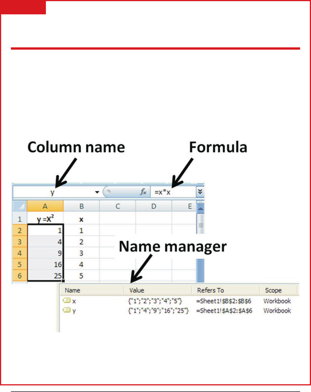
VM–C

FORMULAS

Formulas begin with an equal sign and use cell references

as much as possible.

Lesson: Spreadsheets: Formatting

Page 17 u www.MyCAERT.com

Formula

Cell Reference

VM–D

ORDER OF OPERATIONS

The order of operations is the sequence of calculations in

a formula.

Lesson: Spreadsheets: Formatting

Page 18 u www.MyCAERT.com

VM–E

FORMULA USE GUIDELINE

Even if there is more than one way to perform a

calculation, always use the most efficient form of a

formula.

Lesson: Spreadsheets: Formatting

Page 19 u www.MyCAERT.com

VM–F

FUNCTIONS

A function is an expression that performs common

calculations and returns a single value. Arguments are the

values that functions use to perform calculations.

Lesson: Spreadsheets: Formatting

Page 20 u www.MyCAERT.com

=SUM(D4,E5,F8)

Function

Arguments

VM–G

FORMULA ERROR MESSAGE

A circular reference is a formula in a cell that directly or

indirectly refers to its own cell.

Lesson: Spreadsheets: Formatting

Page 21 u www.MyCAERT.com

The total should be of cells B4,

B5, B6, and B7.

Cell B8 is the cell where the

answer (SUM) is to appear.

Including Cell B8 in the

formula results in a circular

reference.

A formula cannot reference the

cell in which it is stored.

VM–H

COPYING FORMULAS

When the same basic formula

is needed, users can copy that

formula instead of keying it

repeatedly.

Lesson: Spreadsheets: Formatting

Page 22 u www.MyCAERT.com

Selected cell

Fill handle

Formula

Drag fill handle

across cells

Fill handle

LS–A

Name ________________________________________

Compare Spreadsheets:

Microsoft Office Excel and

Google Sheets

Purpose

The purpose of this activity is to compare and contrast two spreadsheet programs: Microsoft

Office Excel and Google Sheets.

Objectives

1. Review available information about MS Excel and Google Sheets programs.

2. Document your comparisons and contrasts of two spreadsheet programs based on your

selection of five key features.

3. Write a brief summary of your recommendations for business and for personal use.

4. Share your findings with your instructor and the class.

Materials

lab sheet

pen or pencil

device with Internet access

Procedure

1. TASK #1: Review the listed YouTube links to evaluate Excel and Google Sheets features

and benefits.

a. “Google Sheets versus MS Excel” at https://www.youtube.com/watch?v=ZBxlsuqTEtQ

Lesson: Spreadsheets: Formatting

Page 23 u www.MyCAERT.com

b. “MS Excel vs Google Sheet - Seven Ways Excel Beats Sheets” at

https://www.youtube.com/watch?v=GFfevN2wje4

c. “Excel Online vs. Google Sheets” at https://www.youtube.com/watch?v=lf3UsTx-lOQ

d. “A 10 Minute Comparison: Office 365 vs Google’s G Suite - WorkTools #32 by

Christoph Magnussen” at https://www.youtube.com/watch?v=bqFioqQogS4

2. TASK #2: Using an Internet search engine, conduct additional research that compares

these spreadsheet packages. Some suggested links include:

a. “Microsoft Excel vs. Google Sheets: Which is better for Business?” at

https://www.computerworld.com/article/3215114/office-software/microsoft-excel-vs-

google-sheets-which-works-better-for-business.html

b. “Microsoft Excel vs. Google Sheets: The Spreadsheet Showdown” at

https://www.process.st/microsoft-excel-vs-google-sheets/

3. TASK #3: Based on your research, select five (5) key spreadsheet features and

summarize your findings in the table provided below:

Feature Microsoft Excel Google Sheets

Lesson: Spreadsheets: Formatting

Page 24 u www.MyCAERT.com

Feature Microsoft Excel Google Sheets

4. TASK #4: Conclusion: Based on your research, which program would you recommend

for business use? What explains your recommendation?

5. TASK #5: Conclusion: Based on your research, which program would you recommend

for personal use? What explains your recommendation?

6. Share your findings with your instructor and the class.

7. Turn your completed lab sheet in to your instructor.

Lesson: Spreadsheets: Formatting

Page 25 u www.MyCAERT.com

LS–B

Name ________________________________________

Order of Operations

Purpose

The purpose of this lab activity is to demonstrate order of operations for formula composition.

Objectives

1. Manually apply the order of operations to provided equations.

2. Create formulas using cell references.

Materials

lab sheet

pen or pencil

device with Excel software

Procedure

1. Apply the order of operations to the following equations. Record your answers next to

each set of numbers and operators. Show your calculations

Equation Calculations and Answer

a. =3+7^2

b. =2+6*4/12

c. =5*4+8–10

Lesson: Spreadsheets: Formatting

Page 26 u www.MyCAERT.com

Equation Calculations and Answer

d. =5*(4+8)–10

e. =20+3*2^2–6

f. =22–11+9+4–12

2. Use the following portion of an

Excel spreadsheet to (1) write

formulas using cell references that

will perform the following

calculations and (2) perform the

calculation by hand or use a

calculator to determine answers

for the following:

a. 20 / 60

b. 20 * 60

c. 60 – 20

d. 60+20*20

e. 60 – 20 + (20 + 20)

f. 60 / 0

3. Turn your completed lab sheet in to your instructor.

Lesson: Spreadsheets: Formatting

Page 27 u www.MyCAERT.com

LS–B: Teacher Information Sheet

Order of Operations

1. Apply the order of operations to the following equations. Student answers would be

similar to the following.

a. ANSWER: 52

First, calculate7^2=49.Then, add 3 to total 52.

b. ANSWER: 10

First,6*4=24.Then, divide by 12 for an answer of 2. Next, add 2 and 6 for an

answer of 10.

c. ANSWER: 18

First,5*4=20.Then, add 8 to get 28. Finally, subtract 10 for the answer: 18.

d. ANSWER: 50

Parentheses are calculated first: so,4+8=12.Then, multiply by 5 with a result of 60.

Finally, subtract 10 to get the answer: 50.

e. ANSWER: 26

Exponents are first, so2^2=4.Then, multiply by 3 to get 12. Next, add 20 for total

of 32. Finally, subtract 6 for answer: 26.

f. ANSWER: 12

All operators are at the same level, so working left to right: 22 – 11 = 11. Then, add 9 to

get 20. Next, add 4 to get 24. Finally, subtract 12 for answer: 12.

2. Remind students that:

• All formulas begin with the “=” sign.

• Cell B3 contains 20.

• Cell C4 contains 60.

Lesson: Spreadsheets: Formatting

Page 28 u www.MyCAERT.com

Formulas Using

Cell References Calculation Process

a. =B3/C4 Divide contents of cell B3 by contents of C4.

ANSWER: .33333

b. =B3*C4 Multiply contents of cell B3 by contents of C4.

ANSWER: 1200

c. =C4–B3 Subtract contents of B3 from contents of C4.

ANSWER: 40

d. =C4+B3*B3 Add contents of C4 to product of B3 * B3; first multiply 20 by 20 for answer of

400. Then, add 60, resulting in 460.

ANSWER: 460

e. =C4–B3+(B3+B3); 80 Take content of C4 and subtract content of B3. Then add sum of B3 and B3;

calculate parentheses first, adding 20 and 20 for total of 40. Next, work left-to-

right, 60 – 20 = 40. Finally, add the previously calculated 40 for an answer of 80.

ANSWER: 80

f. =C4/0 Divide contents of C4 by zero. Cannot divide by 0.

ANSWER: No valid answer exists.

Lesson: Spreadsheets: Formatting

Page 29 u www.MyCAERT.com

LS–C

Name ________________________________________

Writing and Using Formulas

Purpose

The purpose of this lab activity is to practice writing and manipulating formulas from provided

spreadsheet data.

Objectives

1. Compose Excel formulas to accomplish the given spreadsheet calculation task.

2. Write Excel spreadsheet formulas using cell references.

Materials

lab sheet

pen or pencil

Procedure

1. Use this spreadsheet image to complete the following tasks.

Lesson: Spreadsheets: Formatting

Page 30 u www.MyCAERT.com

a. Write the formula for cell F4 to calculate the total of Julia’s scores shown on row 4.

Use individual cell references and + signs to write this formula.

b. Write the formula for cell F5 to calculate the total of Max’s scores shown on row 5.

Use a function and a range of cells to write this formula.

c. Write the formula for cell F6 to calculate the total of Omar’s scores shown on row 6.

Use a function and individual cell references to write this formula.

d. Write the formula for cell G4 to calculate the average of Julia’s scores shown on row

4. Use a function and range of cells to write this formula.

e. The formula just written for cell G4 needs to be copied into cells G5:G8. Explain how

this formula can easily be copied into these other cells.

2. Turn your completed lab sheet in to your instructor.

Lesson: Spreadsheets: Formatting

Page 31 u www.MyCAERT.com

LS–C: Teacher Information Sheet

Writing and Using Formulas

a. =B4+C4+D4+E4

b. =SUM(B4:E4)

c. =SUM(B4, C4, D4, E4)

d. =AVERAGE(B4:E4)

e. Click on cell G4 to select it. Hold the mouse pointer/track pad cursor over the fill handle

at the bottom right corner of the selected cell. Drag the mouse/track pad down cells G5

through G8 and release. Each cell is filled with the formula relative to the row copied to.

Lesson: Spreadsheets: Formatting

Page 32 u www.MyCAERT.com