Microsoft Word - master_pmc_vol

NOT MEASUREMENT

SENSITIVE

MIL-HDBK-17-1F

Volume 1 of 5

17 JUNE 2002

Superseding

MIL-HDBK-17-1E

23 JANUARY 1997

DEPARTMENT OF DEFENSE

HANDBOOK

COMPOSITE MATERIALS HANDBOOK

VOLUME 1. POLYMER MATRIX COMPOSITES

GUIDELINES FOR CHARACTERIZATION

OF STRUCTURAL MATERIALS

This handbook is for guidance only. Do not cite this document as a requirement.

AMSC N/A AREA CMPS

DISTRIBUTION STATEMENT A. Approved for public release; distribution unlimited.

MIL-HDBK-17-1F

Volume 1, Foreword / Table of Contents

FOREWORD

1. This Composite Materials Handbook Series, MIL-HDBK-17, are approved for use by all Departments

and Agencies of the Department of Defense.

2. This handbook is for guidance only. This handbook cannot be cited as a requirement. If it is, the con-

tractor does not have to comply. This mandate is a DoD requirement only; it is not applicable to the

Federal Aviation Administration (FAA) or other government agencies.

3. Every effort has been made to reflect the latest information on polymer (organic), metal, and ceramic

composites. The handbook is continually reviewed and revised to ensure its completeness and cur-

rentness. Documentation for the secretariat should be directed to: Materials Sciences Corporation,

MIL-HDBK-17 Secretariat, 500 Office Center Drive, Suite 250, Fort Washington, PA 19034.

4. MIL-HDBK-17 provides guidelines and material properties for polymer (organic), metal, and ceramic

matrix composite materials. The first three volumes of this handbook currently focus on, but are not

limited to, polymeric composites intended for aircraft and aerospace vehicles. Metal matrix compos-

ites (MMC) and ceramic matrix composites (CMC), including carbon-carbon composites (C-C) are

covered in Volume 4 and Volume 5 , respectively.

5. This standardization handbook has been developed and is being maintained as a joint effort of the

Department of Defense and the Federal Aviation Administration.

6. The information contained in this handbook was obtained from materials producers, industry, reports

on Government sponsored research, the open literature, and by contact with research laboratories

and those who participate in the MIL-HDBK-17 coordination activity.

7. All information and data contained in this handbook have been coordinated with industry and the U.S.

Army, Navy, Air Force, NASA, and Federal Aviation Administration prior to publication.

8. Copies of this document and revisions thereto may be obtained from the Document Automation and

Production Service (DAPS), Bldg. 4D, (DODSSP/ASSIST), 700 Robbins Avenue, Philadelphia, PA

19111-5094.

9. Beneficial comments (recommendations, additions, deletions) and any pertinent data which may be of

use in improving this document should be addressed to: U.S. Army Research Laboratory, Weapons

and Materials Research Directorate, Attn: AMSRL-WM-MA, Aberdeen Proving Ground, MD 21005-

5069, by using the Standardization Document Improvement Proposal (DD Form 1426) appearing at

the end of this document or by letter.

MIL-HDBK-17-1F

Volume 1, Foreword / Table of Contents

iii

CONTENTS

Page

Foreword.....................................................................................................................................................ii

Summary of Changes ............................................................................................................................. xvii

CHAPTER 1

OBJECTIVES.................................................................................................................. 1

1.1 INTRODUCTION........................................................................................................................ 1

1.2 PURPOSE.................................................................................................................................. 1

1.3 SCOPE....................................................................................................................................... 2

1.3.1 Strength properties and allowables data ......................................................................... 3

1.3.2 Volume 1: Guidelines for Characterization of Structural Materials ................................. 3

1.3.3 Volume 2: Material Properties ........................................................................................ 3

1.3.4 Volume 3: Materials Usage, Design, and Analysis Guidelines....................................... 4

1.4 USE OF THE DOCUMENT AND LIMITATIONS ........................................................................ 4

1.4.1 Roadmaps for use of Volumes 1 - 3 ................................................................................ 4

1.4.2 Source of information..................................................................................................... 16

1.4.3 Use of data and guidelines in applications .................................................................... 16

1.4.4 Strength properties and allowables terminology............................................................ 16

1.4.5 Use of references .......................................................................................................... 16

1.4.6 Use of tradenames and product names ........................................................................ 17

1.4.7 Toxicity, health hazards, and safety............................................................................... 17

1.4.8 Ozone depleting chemicals............................................................................................ 17

1.5 APPROVAL PROCEDURES.................................................................................................... 17

1.6 SYMBOLS, ABBREVIATIONS, AND SYSTEMS OF UNITS.................................................... 18

1.6.1 Symbols and abbreviations............................................................................................ 18

1.6.1.1 Constituent properties...................................................................................... 23

1.6.1.2 Laminae and laminates ................................................................................... 23

1.6.1.3 Subscripts ........................................................................................................ 24

1.6.1.4 Superscripts..................................................................................................... 25

1.6.1.5 Acronyms......................................................................................................... 26

1.6.2 System of units .............................................................................................................. 27

1.7 DEFINITIONS........................................................................................................................... 29

REFERENCES ................................................................................................................................... 50

CHAPTER 2

GUIDELINES FOR PROPERTY TESTING OF COMPOSITES ..................................... 1

2.1 INTRODUCTION........................................................................................................................ 1

2.1.1 Building-block approach to substantiation of composite structures................................. 1

2.1.2 Test levels and data uses ................................................................................................ 2

2.1.2.1 Structural complexity levels ............................................................................... 2

2.1.2.2 Data application categories ............................................................................... 3

2.1.2.3 Test program definition ...................................................................................... 4

2.2 TEST PROGRAM PLANNING................................................................................................... 5

2.2.1 Overview.......................................................................................................................... 5

2.2.2 Baseline and alternate approaches for statistically-based properties ............................. 6

2.2.3 Issues of data equivalence .............................................................................................. 6

2.2.4 Test method selection...................................................................................................... 7

2.2.5 Population sampling and sizing ......................................................................................11

2.2.5.1 Sample size selection.......................................................................................11

2.2.5.2 Batch quantity effects on ANOVA .................................................................... 12

MIL-HDBK-17-1F

Volume 1, Foreword / Table of Contents

2.2.6 Material and processing variation, specimen preparation and NDE ............................. 13

2.2.6.1 Materials and material processing................................................................... 13

2.2.6.2 Specimen preparation and NDE...................................................................... 16

2.2.7 Moisture absorption and conditioning factors................................................................ 16

2.2.7.1 Moisture diffusivity ........................................................................................... 18

2.2.7.2 Moisture equilibrium content............................................................................ 18

2.2.7.3 Conditioning and test environment.................................................................. 20

2.2.8 Material operational limit (MOL)..................................................................................... 20

2.2.8.1 Steam pressure delamination.......................................................................... 24

2.2.8.2 MOL considerations for high temperature composite systems ....................... 24

2.2.8.3 Hot Wet Testing - Report Moisture Content at Failure..................................... 27

2.2.9 Nonambient testing........................................................................................................ 29

2.2.10 Unidirectional lamina properties from laminates............................................................ 29

2.2.11 Data normalization......................................................................................................... 29

2.2.12 Data documentation....................................................................................................... 29

2.2.13 Application specific testing needs.................................................................................. 31

2.3 RECOMMENDED TEST MATRICES....................................................................................... 31

2.3.1 Material screening test matrices.................................................................................... 31

2.3.1.1 Mechanical property screening........................................................................ 31

2.3.1.2 Mechanical property screening for high-temperature material systems.......... 32

2.3.1.3 Fluid sensitivity screening................................................................................ 33

2.3.2 Material qualification test matrices ................................................................................ 38

2.3.2.1 Constituent test matrix..................................................................................... 38

2.3.2.2 Prepreg test matrix .......................................................................................... 38

2.3.2.3 Lamina test matrices........................................................................................ 39

2.3.2.4 Filament-wound materials test matrix.............................................................. 41

2.3.3 Material acceptance test matrices ................................................................................. 42

2.3.4 Alternate material equivalence test matrices................................................................. 42

2.3.4.1 Qualification of alternate source composite materials..................................... 42

2.3.4.1.1 Introduction............................................................................................. 42

2.3.4.1.2 Goal and approach................................................................................. 42

2.3.4.1.3 Material compatibility.............................................................................. 43

2.3.4.1.4 Key material or structural performance parameters............................... 43

2.3.4.1.5 Success criteria...................................................................................... 43

2.3.4.1.6 Lamina-level test matrices for alternate material assessment............... 45

2.3.4.1.7 Laminate-level test matrices for alternate material assessment............ 48

2.3.4.1.8 Alternate material evaluation summary.................................................. 48

2.3.4.2 Evaluation of changes made to previously qualified materials........................ 48

2.3.4.2.1 Modification categories........................................................................... 50

2.3.4.2.2 Actions required for each modification category.................................... 51

2.3.4.2.3 Implementation....................................................................................... 51

2.3.4.2.4 Validation test matrices .......................................................................... 56

2.3.5 Generic laminate/structural element test matrices ........................................................ 56

2.3.5.1 Introduction ...................................................................................................... 56

2.3.5.2 Overview.......................................................................................................... 58

2.3.5.2.1 Laminate strength test matrix................................................................. 58

2.3.5.2.2 Bolt bearing and bearing/bypass strength test matrix............................ 60

2.3.6 Alternate approaches to basis values............................................................................ 64

2.3.6.1 Lamina mechanical property test matrix for regression analysis .................... 64

2.3.7 Data substantiation for use of basis values from MIL-HDBK-17 or other large

databases ...................................................................................................................... 66

2.4 DATA REDUCTION AND DOCUMENTATION......................................................................... 67

2.4.1 Introduction ....................................................................................................................67

2.4.2 Lamina properties from laminates ................................................................................. 67

2.4.2.1 Methodology .................................................................................................... 68

2.4.2.2 Tension strength tests...................................................................................... 69

MIL-HDBK-17-1F

Volume 1, Foreword / Table of Contents

2.4.2.3 Compression strength tests............................................................................. 70

2.4.2.4 Other properties............................................................................................... 70

2.4.3 Data normalization......................................................................................................... 70

2.4.3.1 Normalization theory........................................................................................ 71

2.4.3.2 Normalization methodology............................................................................. 71

2.4.3.3 Practical application of normalization .............................................................. 74

2.4.4 Dispositioning of Outlier Data ........................................................................................ 75

2.4.5 Data documentation....................................................................................................... 78

2.5 MATERIAL TESTING FOR SUBMISSION OF DATA TO MIL-HDBK-17 ................................. 78

2.5.1 Introduction ....................................................................................................................78

2.5.2 Material and process specification requirements .......................................................... 80

2.5.3 Sampling requirements.................................................................................................. 80

2.5.3.1 Additional requirements for B and A data classes ........................................... 81

2.5.3.2 Data pooling..................................................................................................... 81

2.5.4 Conditioning requirements............................................................................................. 82

2.5.5 Test method requirements ............................................................................................. 82

2.5.6 Data documentation requirements................................................................................. 82

2.5.7 Data normalization......................................................................................................... 87

2.5.8 Statistical analysis.......................................................................................................... 87

2.5.9 Mechanical properties of laminae and laminates .......................................................... 87

2.5.9.1 Unidirectional properties from laminates ........................................................ 87

2.5.9.2 Strength and strain-to-failure ........................................................................... 87

2.5.9.3 Elastic moduli, Poisson's ratios, and stress/strain curves............................... 88

2.5.10 Chemical properties....................................................................................................... 88

2.5.11 Physical properties of laminae and laminates ............................................................... 88

2.5.11.1 Density............................................................................................................. 88

2.5.11.2 Composition..................................................................................................... 88

2.5.11.3 Equilibrium moisture content ........................................................................... 88

2.5.11.4 Moisture diffusivity ........................................................................................... 88

2.5.11.5 Coefficient of moisture expansion ................................................................... 88

2.5.11.6 Glass transition temperature ........................................................................... 88

2.5.12 Thermal properties......................................................................................................... 89

2.5.12.1 Coefficient of thermal expansion ..................................................................... 89

2.5.12.2 Specific heat .................................................................................................... 89

2.5.12.3 Thermal conductivity........................................................................................ 89

2.5.12.4 Thermal diffusivity............................................................................................ 89

2.5.13 Electrical properties ....................................................................................................... 90

2.5.14 Fatigue 90

REFERENCES ................................................................................................................................... 92

CHAPTER 3

EVALUATION OF REINFORCEMENT FIBERS ............................................................. 1

3.1 INTRODUCTION........................................................................................................................ 1

3.2 CHEMICAL TECHNIQUES ........................................................................................................ 1

3.2.1 Elemental analysis........................................................................................................... 1

3.2.2 Titration............................................................................................................................ 2

3.2.3 Fiber structure.................................................................................................................. 2

3.2.4 Fiber surface chemistry ................................................................................................... 2

3.2.5 Sizing content and composition....................................................................................... 5

3.2.6 Moisture content .............................................................................................................. 5

3.2.7 Thermal stability and oxidative resistance....................................................................... 5

3.2.8 Chemical resistance ........................................................................................................ 5

3.3 PHYSICAL TECHNIQUES (INTRINSIC) ................................................................................... 6

3.3.1 Filament diameter............................................................................................................ 6

3.3.2 Density of fibers ...............................................................................................................6

MIL-HDBK-17-1F

Volume 1, Foreword / Table of Contents

3.3.2.1 Overview............................................................................................................ 6

3.3.2.2 ASTM D 3800, Standard Test Method for Density of High-Modulus

Fibers................................................................................................................. 7

3.3.2.3 Recommended procedure changes to Section 6.6.4.4.1 (helium

pycnometry) for use in measuring fiber density................................................. 8

3.3.2.4 Density test methods for MIL-HDBK-17 data submittal..................................... 8

3.3.3 Electrical resistivity ..........................................................................................................8

3.3.4 Coefficient of thermal expansion ..................................................................................... 9

3.3.5 Thermal conductivity........................................................................................................ 9

3.3.6 Specific heat .................................................................................................................... 9

3.3.7 Thermal transition temperatures...................................................................................... 9

3.4 PHYSICAL TECHNIQUES (EXTRINSIC) .................................................................................. 9

3.4.1 Yield of yarn, strand, or roving......................................................................................... 9

3.4.2 Cross-sectional area of yarn or tow............................................................................... 10

3.4.3 Twist of yarn...................................................................................................................10

3.4.4 Fabric construction ........................................................................................................ 10

3.4.5 Fabric areal density ....................................................................................................... 10

3.5 MECHANICAL TESTING OF FIBERS ..................................................................................... 10

3.5.1 Tensile properties........................................................................................................... 10

3.5.1.1 Filament tensile testing.....................................................................................11

3.5.1.2 Tow tensile testing ............................................................................................11

3.5.1.3 Fiber properties from unidirectional laminate tests.......................................... 14

3.5.2 Filament compression testing........................................................................................ 14

3.6 TEST METHODS ..................................................................................................................... 14

3.6.1 Determination of pH....................................................................................................... 14

3.6.1.1 Scope............................................................................................................... 14

3.6.1.2 Apparatus ........................................................................................................ 14

3.6.1.3 Procedure ........................................................................................................ 15

3.6.2 Determination of amount of sizing on carbon fibers ...................................................... 15

3.6.2.1 Scope............................................................................................................... 15

3.6.2.2 Apparatus ........................................................................................................ 15

3.6.2.3 Materials .......................................................................................................... 16

3.6.2.4 Procedure ........................................................................................................ 16

3.6.2.5 Calculation....................................................................................................... 16

3.6.2.6 Preparation of crucibles for reuse.................................................................... 17

3.6.3 Determination of moisture content or moisture regain .................................................. 17

3.6.3.1 Scope............................................................................................................... 17

3.6.3.2 Apparatus ........................................................................................................ 17

3.6.3.3 Sample preparation ......................................................................................... 17

3.6.3.4 Procedure ........................................................................................................ 17

3.6.3.5 Calculations ..................................................................................................... 18

3.6.4 Determination of fiber diameter ..................................................................................... 18

3.6.4.1 Description and application ............................................................................. 18

3.6.4.2 Apparatus ........................................................................................................ 18

3.6.4.3 Calibration........................................................................................................ 20

3.6.4.4 Prepare slide.................................................................................................... 20

3.6.4.5 Measuring procedure....................................................................................... 20

3.6.4.6 Calculation....................................................................................................... 21

3.6.5 Determination of electrical resistivity ............................................................................. 21

3.6.5.1 Scope............................................................................................................... 21

3.6.5.2 Apparatus ........................................................................................................ 21

3.6.5.3 Sample preparation ......................................................................................... 21

3.6.5.4 Procedure ........................................................................................................ 21

3.6.5.5 Calculation....................................................................................................... 21

3.6.5.6 Calibration and maintenance........................................................................... 22

3.6.5.7 Definition of units of measurement.................................................................. 22

MIL-HDBK-17-1F

Volume 1, Foreword / Table of Contents

vii

REFERENCES ................................................................................................................................... 23

CHAPTER 4

MATRIX CHARACTERIZATION ..................................................................................... 1

4.1 INTRODUCTION........................................................................................................................ 1

4.2 MATRIX SPECIMEN PREPARATION........................................................................................ 1

4.2.1 Introduction ...................................................................................................................... 1

4.2.2 Thermoset polymers ........................................................................................................ 2

4.2.3 Thermoplastic polymers................................................................................................... 3

4.2.4 Specimen machining........................................................................................................ 3

4.3 CONDITIONING AND ENVIRONMENTAL EXPOSURE ........................................................... 4

4.4 CHEMICAL ANALYSIS TECHNIQUES...................................................................................... 4

4.4.1 Elemental analysis........................................................................................................... 4

4.4.2 Functional group and wet chemical analysis................................................................... 4

4.4.3 Spectroscopic analysis .................................................................................................... 4

4.4.4 Chromatographic analysis ............................................................................................... 6

4.4.5 Molecular weight and molecular weight distribution analysis.......................................... 6

4.4.6 General scheme for resin material characterization........................................................ 7

4.5 THERMAL/PHYSICAL ANALYSIS AND PROPERTY TESTS ................................................. 14

4.5.1 Introduction ....................................................................................................................15

4.5.2 Thermal analysis............................................................................................................ 15

4.5.3 Rheological analysis...................................................................................................... 16

4.5.4 Morphology .................................................................................................................... 17

4.5.5 Density/specific gravity .................................................................................................. 17

4.5.5.1 Overview.......................................................................................................... 17

4.5.5.2 Recommended procedure changes to Sections 6.6.4.2, 6.6.4.3 and

6.6.4.4 (D 792, D 1505 and helium pycnometry) for use in measuring

cured resin density........................................................................................... 18

4.5.5.3 Density test methods for MIL-HDBK-17 data submittal................................... 18

4.5.6 Volatiles content............................................................................................................. 19

4.5.7 Moisture content ............................................................................................................ 19

4.6 STATIC MECHANICAL PROPERTY TESTS........................................................................... 20

4.6.1 Introduction ....................................................................................................................20

4.6.2 Tension........................................................................................................................... 20

4.6.2.1 Introduction ...................................................................................................... 20

4.6.2.2 Specimen preparation...................................................................................... 20

4.6.2.3 Test apparatus and instrumentation ................................................................ 21

4.6.2.4 Tensile test methods for MIL-HDBK-17 data submittal.................................... 22

4.6.3 Compression.................................................................................................................. 22

4.6.3.1 Introduction ...................................................................................................... 23

4.6.3.2 Specimen preparation...................................................................................... 23

4.6.3.3 Test apparatus and instrumentation ................................................................ 23

4.6.3.4 Limitations........................................................................................................ 24

4.6.3.5 Compressive test methods for MIL-HDBK-17 data submittal.......................... 24

4.6.4 Shear ............................................................................................................................. 24

4.6.4.1 Test methods available .................................................................................... 24

4.6.4.2 Torsion specimen preparation ......................................................................... 25

4.6.4.3 Iosipescu shear specimen preparation............................................................ 25

4.6.4.4 Test apparatus and instrumentation ................................................................ 25

4.6.4.5 Limitations........................................................................................................ 25

4.6.4.6 Shear testing methods for MIL-HDBK-17 data submittal ................................ 25

4.6.5 Flexure........................................................................................................................... 26

4.6.5.1 Introduction ...................................................................................................... 26

4.6.5.2 Specimen preparation...................................................................................... 26

4.6.5.3 Test apparatus and instrumentation ................................................................ 26

MIL-HDBK-17-1F

Volume 1, Foreword / Table of Contents

viii

4.6.5.4 Flexural test methods for MIL-HDBK-17 data submittal.................................. 27

4.6.6 Impact ............................................................................................................................ 27

4.6.7 Hardness........................................................................................................................27

4.7 FATIGUE TESTING.................................................................................................................. 27

4.8 TESTING OF VISCOELASTIC PROPERTIES ........................................................................ 28

REFERENCES ................................................................................................................................... 29

CHAPTER 5

PREPREG MATERIALS CHARACTERIZATION ........................................................... 1

5.1 INTRODUCTION........................................................................................................................ 1

5.2 CHARACTERIZATION TECHNIQUES - OVERVIEW................................................................ 1

5.3 SAMPLING................................................................................................................................. 2

5.4 PHYSICAL CHARACTERISTICS AND PROPERTY TESTS..................................................... 2

5.4.1 Physical description of reinforcement.............................................................................. 2

5.4.1.1 Alignment........................................................................................................... 2

5.4.1.2 Gaps .................................................................................................................. 2

5.4.1.3 Width.................................................................................................................. 3

5.4.1.4 Length................................................................................................................ 3

5.4.1.5 Edges................................................................................................................. 3

5.4.1.6 Splices ............................................................................................................... 3

5.4.2 Resin content...................................................................................................................3

5.4.3 Fiber content.................................................................................................................... 3

5.4.4 Volatiles content...............................................................................................................3

5.4.5 Moisture content .............................................................................................................. 4

5.4.6 Inorganic fillers and additives content ............................................................................. 4

5.4.7 Areal weight ..................................................................................................................... 4

5.4.8 Tack and drape ................................................................................................................ 4

5.4.9 Resin flow ........................................................................................................................ 4

5.4.10 Gel time 4

5.5 TEST METHODS ....................................................................................................................... 4

5.5.1 Resin extraction procedure for epoxy resin prepregs...................................................... 4

5.5.2 Procedure for HPLC/HPSEC analysis of glass, aramid, and graphite fiber

prepregs........................................................................................................................... 6

5.5.2.1 Reverse phase HPLC analysis.......................................................................... 6

5.5.2.2 Size Exclusion Chromatography (SEC) analysis .............................................. 7

5.5.3 Procedure for Fourier transform infrared spectroscopy (FTIR) ....................................... 7

5.5.4 Procedure for differential scanning calorimetry (DSC) .................................................... 7

5.5.5 Procedure for dynamic mechanical analysis (DMA)........................................................ 8

5.5.6 Procedure for rheological characterization...................................................................... 8

REFERENCES ..................................................................................................................................... 9

CHAPTER 6

LAMINA, LAMINATE, AND SPECIAL FORM CHARACTERIZATION .......................... 1

6.1 INTRODUCTION........................................................................................................................ 1

6.2 SPECIMEN PREPARATION ...................................................................................................... 1

6.2.1 Introduction ...................................................................................................................... 1

6.2.2 Traceability....................................................................................................................... 2

6.2.3 Test article fabrication...................................................................................................... 2

6.2.4 Specimen fabrication ....................................................................................................... 3

6.3 CONDITIONING AND ENVIRONMENTAL EXPOSURE ........................................................... 4

6.3.1 Introduction ...................................................................................................................... 4

6.3.2 Fixed-time conditioning.................................................................................................... 5

6.3.3 Equilibrium conditioning................................................................................................... 6

6.3.3.1 Accelerating conditioning times......................................................................... 7

MIL-HDBK-17-1F

Volume 1, Foreword / Table of Contents

6.3.3.2

Procedural hints................................................................................................. 8

6.4 INSTRUMENTATION AND CALIBRATION.............................................................................. 10

6.4.1 Introduction ....................................................................................................................10

6.4.2 Test specimen dimensional measurement .................................................................... 10

6.4.2.1 Introduction ...................................................................................................... 10

6.4.2.2 Calibrated microscopes ................................................................................... 10

6.4.2.3 Micrometers..................................................................................................... 10

6.4.2.4 Scaled calipers .................................................................................................11

6.4.2.5 Precision scales................................................................................................11

6.4.2.6 Rulers and tape measures............................................................................... 12

6.4.2.7 Special hole diameter measuring devices ....................................................... 12

6.4.2.8 Calibration of dimensional measurement devices........................................... 12

6.4.3 Load measurement devices........................................................................................... 12

6.4.3.1 Introduction ...................................................................................................... 12

6.4.3.2 Load cells......................................................................................................... 13

6.4.3.2.1 Design and specification considerations................................................ 13

6.4.3.3 Other load measuring systems........................................................................ 14

6.4.3.4 Instrumentation and calibration ....................................................................... 14

6.4.3.5 Precautions...................................................................................................... 15

6.4.4 Strain/displacement measurement devices................................................................... 15

6.4.4.1 Introduction ...................................................................................................... 15

6.4.4.2 LVDT (Linear Variable Differential Transformer) deflectometers..................... 16

6.4.4.3 Contacting extensometers............................................................................... 16

6.4.4.3.1 Contacting extensometers, applications ................................................ 16

6.4.4.4 Bondable resistance strain gages ................................................................... 17

6.4.4.4.1 Strain gage selection.............................................................................. 17

6.4.4.4.2 Surface preparation and bonding of strain gages.................................. 17

6.4.4.4.3 Strain gage circuits................................................................................. 17

6.4.4.4.4 Strain gage instrumentation ................................................................... 18

6.4.4.4.5 Strain gage instrumentation calibration.................................................. 19

6.4.4.5 Other methods................................................................................................. 19

6.4.4.5.1 Optical methods of extensometry........................................................... 19

6.4.4.5.2 Capacitative extensometers................................................................... 20

6.4.4.6 Special considerations for textile composites.................................................. 20

6.4.5 Temperature measurement devices .............................................................................. 20

6.4.5.1 Introduction ...................................................................................................... 20

6.4.5.2 Thermocouples................................................................................................ 20

6.4.5.3 Metallic resistive temperature devices............................................................. 21

6.4.5.4 Thermistors...................................................................................................... 22

6.4.5.5 Bimetallic devices ............................................................................................ 22

6.4.5.6 Liquid expansion devices................................................................................. 22

6.4.5.7 Change-of-state devices.................................................................................. 22

6.4.5.8 Infrared detectors............................................................................................. 23

6.4.5.9 Calibration of temperature measurement devices........................................... 23

6.4.6 Data acquisition systems............................................................................................... 26

6.5 TESTING ENVIRONMENTS.................................................................................................... 26

6.5.1 Introduction ....................................................................................................................26

6.5.2 Laboratory ambient test environment............................................................................ 26

6.5.3 Non-ambient testing environment.................................................................................. 26

6.5.3.1 Introduction ...................................................................................................... 26

6.5.3.2 Subambient testing.......................................................................................... 27

6.5.3.3 Above ambient testing ..................................................................................... 27

6.6 THERMAL/PHYSICAL PROPERTY TESTS............................................................................ 28

6.6.1 Introduction ....................................................................................................................28

6.6.2 Extent of cure................................................................................................................. 28

6.6.3 Glass transition temperature.......................................................................................... 29

MIL-HDBK-17-1F

Volume 1, Foreword / Table of Contents

6.6.3.1

Overview.......................................................................................................... 29

6.6.3.2 T

Measurements............................................................................................. 29

6.6.3.2.1 Differential scanning calorimetry (DSC)................................................. 29

6.6.3.2.2 Thermomechanical analysis (TMA)........................................................ 30

6.6.3.2.3 Dynamic mechanical analysis (DMA)..................................................... 32

6.6.3.3 Glass transition test methods for MIL-HDBK-17 data submittal...................... 33

6.6.3.4 Crystalline melt temperature............................................................................ 33

6.6.4 Density........................................................................................................................... 34

6.6.4.1 Overview.......................................................................................................... 34

6.6.4.2 ASTM D 792, Standard Test Method for Density and Specific Gravity

(Relative Density) of Plastics by Displacement............................................... 34

6.6.4.3 ASTM D 1505, Standard Test Method for Density of Plastics by the

Density-Gradient Technique ............................................................................ 35

6.6.4.4 Use of helium pycnometry to determine density of composites ...................... 36

6.6.4.4.1 Helium pycnometry test procedure for determining composite

density.................................................................................................... 38

6.6.4.5 Summary of helium pycnometry experimental results..................................... 39

6.6.4.6 Density test methods for MIL-HDBK-17 data submittal................................... 40

6.6.5 Cured ply thickness ....................................................................................................... 40

6.6.5.1 Overview.......................................................................................................... 41

6.6.5.2 Thickness measurement using direct means .................................................. 41

6.6.5.3 Thickness measurement using indirect means ............................................... 41

6.6.5.4 SRM 10R-94, SACMA Recommended Method for Fiber Volume,

Percent Resin Volume and Calculated Average Cured Ply Thickness of

Plied Laminates ............................................................................................... 42

6.6.5.5 Cured ply thickness test methods for MIL-HDBK-17 data submittal ............... 42

6.6.6 Fiber volume (V

) fraction .............................................................................................. 42

6.6.6.1 Introduction ...................................................................................................... 42

6.6.6.2 Matrix digestion................................................................................................ 42

6.6.6.3 Ignition loss...................................................................................................... 43

6.6.6.4 Areal weight/thickness..................................................................................... 43

6.6.6.5 Determination of fiber volume using image analysis....................................... 45

6.6.6.5.1 Background ............................................................................................ 45

6.6.6.5.2 Apparatus ............................................................................................... 45

6.6.6.5.3 Specimen preparation ............................................................................ 45

6.6.6.5.4 Image analysis ....................................................................................... 46

6.6.6.5.5 Sources of error...................................................................................... 47

6.6.7 Void volume (V

) fraction ............................................................................................... 48

6.6.7.1 Introduction ...................................................................................................... 48

6.6.7.2 Digestive evaluation......................................................................................... 48

6.6.7.3 Determination of void volume using image analysis ....................................... 49

6.6.7.3.1 Background ............................................................................................ 49

6.6.7.3.2 Sources of Error ..................................................................................... 50

6.6.8 Moisture/diffusivity ......................................................................................................... 52

6.6.8.1 Standard test methods..................................................................................... 53

6.6.8.2 Moisture diffusion property test methods for MIL-HDBK-17 data

submittal........................................................................................................... 54

6.6.9 Dimensional stability (Thermal and Moisture) ............................................................... 54

6.6.9.1 Dimensional stability (thermal) ........................................................................ 55

6.6.9.1.1 Introduction............................................................................................. 55

6.6.9.1.2 Existing test methods ............................................................................. 55

6.6.9.1.3 Test specimens....................................................................................... 56

6.6.9.1.4 Test apparatus and instrumentation ....................................................... 57

6.6.9.1.5 CTE test methods for MIL-HDBK-17 data submittal .............................. 57

6.6.9.2 Dimensional stability (moisture)....................................................................... 58

6.6.9.2.1 Introduction............................................................................................. 58

MIL-HDBK-17-1F

Volume 1, Foreword / Table of Contents

6.6.9.2.2

Specimen preparation ............................................................................ 59

6.6.9.2.3 Test apparatus and instrumentation ....................................................... 59

6.6.9.2.4 CME test methods for MIL-HDBK-17 data submittal ............................. 60

6.6.10 Thermal conductivity...................................................................................................... 60

6.6.10.1 Introduction ...................................................................................................... 60

6.6.10.2 Available methods ........................................................................................... 60

6.6.10.2.1 ASTM C177-97....................................................................................... 61

6.6.10.2.2 ASTM E1225-99..................................................................................... 62

6.6.10.2.3 ASTM C518-98....................................................................................... 63

6.6.10.2.4 Fourier thermal conductivity test method for flat plates ......................... 64

6.6.10.3 Thermal conductivity test methods for MIL-HDBK-17 data ............................. 68

6.6.11 Specific heat .................................................................................................................. 68

6.6.11.1 Introduction ...................................................................................................... 68

6.6.11.2 Available method ............................................................................................. 68

6.6.11.2.1 ASTM E1269-95..................................................................................... 68

6.6.11.3 Specific heat test methods for MIL-HDBK-17 data submittal .......................... 70

6.6.12 Thermal diffusivity.......................................................................................................... 70

6.6.12.1 Introduction ...................................................................................................... 70

6.6.12.2 Available test methods..................................................................................... 71

6.6.12.2.1 ASTM E1461-92..................................................................................... 71

6.6.12.2.2 ASTM C714-85....................................................................................... 76

6.6.12.3 Thermal diffusivity test methods for MIL-HDBK-17 data submittal.................. 76

6.6.13 Outgassing..................................................................................................................... 76

6.6.14 Absorptivity and emissivity............................................................................................. 77

6.6.15 Thermal cycling.............................................................................................................. 77

6.6.16 Microcracking................................................................................................................. 77

6.6.16.1 Introduction ...................................................................................................... 77

6.6.16.2 Microcracking due to the manufacturing process............................................ 77

6.6.16.3 Microcracking due thermal cycling .................................................................. 78

6.6.16.4 Microcracking due to mechanical loading/cycling ........................................... 78

6.6.17 Thermal oxidative stability (TOS)................................................................................... 78

6.6.18 Flammability and smoke generation.............................................................................. 78

6.6.18.1 Introduction ...................................................................................................... 78

6.6.18.2 Fire growth test methods ................................................................................. 78

6.6.18.2.1 ASTM E 84 - Surface burning characteristics of building materials....... 79

6.6.18.2.2 ASTM E 162 - Surface flammability of materials using a radiant

heat energy source................................................................................. 80

6.6.18.2.3 ISO 9705 fire test – full-scale room test for surface products................ 81

6.6.18.2.4 ASTM E 1321 - Determining material ignition and flame spread

properties ............................................................................................... 81

6.6.18.3 Smoke and toxicity test methods..................................................................... 82

6.6.18.3.1 ASTM E 662 - Specific optical density of smoke generated by solid

materials................................................................................................. 82

6.6.18.3.2 NFPA 269 - Developing toxic potency data for use in fire hazard

modeling................................................................................................. 83

6.6.18.4 Heat release test methods............................................................................... 84

6.6.18.4.1 ASTM E-1354 - Heat and visible smoke release rates for materials

and products using an oxygen consumption calorimeter....................... 84

6.6.18.4.2 ASTM E 906 – Heat and visible smoke release rates for materials

and products........................................................................................... 85

6.6.18.5 Fire resistance test methods ........................................................................... 86

6.6.18.5.1 ASTM E-119 - Fire tests for building construction and materials........... 86

6.6.18.5.2 ASTM E-1529 - Determining effects of large hydrocarbon pool

fires on structural members and assemblies and UL 1709 - Rapid

rise fire tests of protection materials for structural steel......................... 87

6.7 ELECTRICAL PROPERTY TESTS.......................................................................................... 87

MIL-HDBK-17-1F

Volume 1, Foreword / Table of Contents

xii

6.7.1

Introduction ....................................................................................................................87

6.7.2 Electrical permittivity...................................................................................................... 88

6.7.3 Dielectric strength .......................................................................................................... 88

6.7.4 Magnetic permeability.................................................................................................... 88

6.7.5 Electromagnetic interference......................................................................................... 88

6.7.6 Electrostatic discharage................................................................................................. 88

6.8 STATIC UNIAXIAL MECHANICAL PROPERTY TESTS.......................................................... 88

6.8.1 Introduction ....................................................................................................................88

6.8.2 Tensile properties........................................................................................................... 89

6.8.2.1 Overview.......................................................................................................... 90

6.8.2.2 In-plane tension test methods ......................................................................... 91

6.8.2.2.1 Straight-sided specimen tension tests.................................................... 91

6.8.2.2.2 Filament-wound tubes............................................................................ 94

6.8.2.2.3 Width tapered specimens:...................................................................... 94

6.8.2.2.4 Split-disk ring tension test ...................................................................... 95

6.8.2.2.5 Sandwich beam test............................................................................... 95

6.8.2.3 Out-of-plane tensile test methods.................................................................... 97

6.8.2.3.1 Introduction............................................................................................. 97

6.8.2.3.2 Direct out-of-plane loading adaptations of ASTM

C 297/C 633/D 2095............................................................................... 97

6.8.2.3.3 Curved beam approach to out-of-plane tensile strength...................... 102

6.8.2.4 Tension test methods for MIL-HDBK-17 data submittal ................................ 102

6.8.3 Compressive properties............................................................................................... 104

6.8.3.1 Overview........................................................................................................ 104

6.8.3.2 In-plane compression tests............................................................................ 105

6.8.3.2.1 ASTM D 3410/D 3410M, Compressive Properties of Polymer

Matrix Composite Materials With Unsupported Gage Section by

Shear Loading...................................................................................... 105

6.8.3.2.2 ASTM D 6484, Compressive Properties of Polymer Matrix

Composite Laminates Using a Combined Loading Compression

(CLC) Test Fixture................................................................................ 106

6.8.3.2.3 ASTM D 5467, Compressive Properties of Unidirectional Polymer

Matrix Composites Using a Sandwich Beam ....................................... 109

6.8.3.2.4 ASTM C 393, Flexural Properties of Flat Sandwich Constructions ......110

6.8.3.2.5 ASTM D 695, Compressive Properties of Rigid Plastics ......................111

6.8.3.2.6 SACMA SRM 1R, Compressive Properties of Oriented Fiber-Resin

Composites ...........................................................................................112

6.8.3.2.7 SACMA SRM 6, Compressive Properties of Oriented Cross-Plied

Fiber-Resin Composites........................................................................113

6.8.3.2.8 Through-thickness compression tests...................................................114

6.8.3.3 Compressive test methods for developing MIL-HDBK-17 data submittal ......114

6.8.4 Shear properties ...........................................................................................................116

6.8.4.1 Overview.........................................................................................................116

6.8.4.2 In-plane shear tests ........................................................................................117

6.8.4.2.1 ±45° tensile shear tests.........................................................................117

6.8.4.2.2 Iosipescu shear test ..............................................................................119

6.8.4.2.3 Rail shear tests..................................................................................... 123

6.8.4.2.4 Ten-degree off-axis shear test.............................................................. 123

6.8.4.2.5 Tube torsion tests................................................................................. 124

6.8.4.3 Out-of-plane shear tests ................................................................................ 125

6.8.4.3.1 Short-beam strength tests.................................................................... 125

6.8.4.3.2 Iosipescu shear test ............................................................................. 126

6.8.4.3.3 ASTM D 3846-79, Test Method for In-Plane Shear Strength of

Reinforced Plastics............................................................................... 126

6.8.4.4 Shear test methods for MIL-HDBK-17 data submittal ................................... 127

6.8.5 Flexural properties ....................................................................................................... 128

MIL-HDBK-17-1F

Volume 1, Foreword / Table of Contents

xiii

6.8.6 Fracture toughness properties..................................................................................... 128

6.8.6.1 Overview........................................................................................................ 128

6.8.6.2 General discussion ........................................................................................ 129

6.8.6.3 Mode I test methods ...................................................................................... 131

6.8.6.3.1 Double cantilever beam (DCB) test, ASTM D 5528............................. 131

6.8.6.3.2 Other mode I tests................................................................................ 133

6.8.6.4 Mode II test methods ..................................................................................... 133

6.8.6.4.1 End notched flexure (ENF) test............................................................ 133

6.8.6.4.2 Other mode II tests............................................................................... 134

6.8.6.5 Mode III test methods .................................................................................... 134

6.8.6.6 Mixed mode test methods ............................................................................. 135

6.8.6.6.1 Mixed mode specimen or crack lap shear (CLS) ................................. 135

6.8.6.6.2 Mixed mode bending (MMB) test ......................................................... 135

6.8.6.6.3 Edge delamination test......................................................................... 136

6.8.6.7 Fracture toughness tests for MIL-HDBK-17 data submittal........................... 137

6.9 UNIAXIAL FATIGUE TESTING .............................................................................................. 137

6.10 MULTIAXIAL MECHANICAL PROPERTY TESTING............................................................. 137

6.11 VISCOELASTIC PROPERTIES TESTS ................................................................................ 138

6.11.1 Introduction .................................................................................................................. 138

6.11.2 Creep and stress relaxation......................................................................................... 138

6.12 FORM-SPECIFIC MECHANICAL PROPERTY TESTS......................................................... 139

6.12.1 Tests unique to filament winding.................................................................................. 139

6.12.1.1 Overview........................................................................................................ 139

6.12.1.2 History............................................................................................................ 139

6.12.1.3 Tension tests for uniaxial material properties ................................................ 140

6.12.1.3.1 Zero degree tension ............................................................................. 140

6.12.1.3.2 Transverse tension............................................................................... 140

6.12.1.4 Compression tests for uniaxial material properties ....................................... 140

6.12.1.4.1 Zero degree compression .................................................................... 140

6.12.1.4.2 Transverse compression...................................................................... 140

6.12.1.5 Shear tests for uniaxial material properties ................................................... 140

6.12.1.5.1 In-plane shear ...................................................................................... 140

6.12.1.5.2 Transverse shear.................................................................................. 140

6.12.1.6 Test methods for MIL-HDBK-17 data submittal ............................................. 140

6.12.2 Tests unique to textiles composites ............................................................................. 141

6.12.2.1 Overview........................................................................................................ 141

6.12.2.2 Background.................................................................................................... 142

6.12.2.3 Fabric and two-dimensional weaves ............................................................. 142

6.12.2.3.1 Physical property tests ......................................................................... 142

6.12.2.3.2 Mechanical testing................................................................................ 143

6.12.2.3.3 Impact considerations .......................................................................... 143

6.12.2.4 Complex braiding considerations .................................................................. 143

6.12.2.4.1 Three-dimensional weave and braids .................................................. 144

6.12.2.4.2 Through the thickness test methods .................................................... 144

6.12.2.5 Test methods for submission to MIL-HDBK-17 ............................................. 144

6.12.3 Tests unique to thick-section composites .................................................................... 145

6.13 SPACE ENVIRONMENTAL EFFECTS ON MATERIAL PROPERTIES................................. 146

6.13.1 Introduction .................................................................................................................. 146

6.13.2 Atomic oxygen ............................................................................................................. 146

6.13.3 Micrometeoroid Debris................................................................................................. 146

6.13.4 Ultraviolet radiation ...................................................................................................... 146

6.13.5 Charged particles......................................................................................................... 146

REFERENCES ................................................................................................................................. 147

MIL-HDBK-17-1F

Volume 1, Foreword / Table of Contents

xiv

CHAPTER 7 STRUCTURAL ELEMENT CHARACTERIZATION........................................................ 1

7.1 INTRODUCTION........................................................................................................................ 1

7.2 SPECIMEN PREPARATION ...................................................................................................... 1

7.2.1 Introduction ...................................................................................................................... 1

7.2.2 Mechanically fastened joint tests..................................................................................... 1

7.2.3 Bonded joint tests ............................................................................................................ 2

7.3 CONDITIONING AND ENVIRONMENTAL EXPOSURE ........................................................... 2

7.3.1 Introduction ...................................................................................................................... 2

7.3.2 General specimen preparation ........................................................................................ 2

7.3.2.1 Strain gaging...................................................................................................... 2

7.3.2.2 Notched laminates and mechanically fastened joint specimens....................... 3

7.3.3 Bonded joints ...................................................................................................................3

7.3.4 Damage characterization specimens .............................................................................. 4

7.3.5 Sandwich Structure.......................................................................................................... 4

7.4 NOTCHED LAMINATE TESTS.................................................................................................. 6

7.4.1 Overview and general considerations ............................................................................. 6

7.4.2 Notched laminate tension ................................................................................................ 7

7.4.2.1 Open-hole tensile test methods......................................................................... 8

7.4.2.2 Filled-hole tensile test methods......................................................................... 8

7.4.3 Notched laminate compression ....................................................................................... 8

7.4.3.1 Open-hole compressive test methods............................................................. 10

7.4.3.2 Filled-hole compressive test methods ..............................................................11

7.4.4 Suggested notched laminate test matrix ........................................................................11

7.4.5 Notched laminate test methods for MIL-HDBK-17 data submittal................................. 13

7.5 MECHANICALLY-FASTENED JOINT TESTS.......................................................................... 13

7.5.1 Overview........................................................................................................................13

7.5.1.1 Definitions ........................................................................................................ 13

7.5.1.2 Failure modes.................................................................................................. 14

7.5.1.3 Design requirements........................................................................................ 15

7.5.2 Bearing Tests ................................................................................................................. 15

7.5.2.1 Overview.......................................................................................................... 15

7.5.2.2 Double shear bearing tests.............................................................................. 16

7.5.2.2.1 ASTM D 953 bearing strength of plastics .............................................. 16

7.5.2.2.2 ASTM D 5961, Procedure A................................................................... 17

7.5.2.3 Single shear bearing tests............................................................................... 19

7.5.2.3.1 Overview ................................................................................................ 19

7.5.2.3.2 ASTM D 5961, Procedure B................................................................... 19

7.5.2.4 Suggested joint bearing test matrices ............................................................. 21

7.5.2.5 Effects of thickness/gaps/shimming................................................................. 25

7.5.2.6 Failure modes.................................................................................................. 27

7.5.3 Bearing/by-pass evaluation ........................................................................................... 30

7.5.3.1 Overview and rationale.................................................................................... 30

7.5.3.2 Specimen design and testing........................................................................... 31

7.5.3.3 Suggested bearing/bypass test matrix ............................................................ 33

7.5.3.4 Data reduction ................................................................................................. 33

7.5.4 Shear-out strength ......................................................................................................... 34

7.5.5 Fastener pull-thru strength (MIL-HDBK-17 test method)............................................... 36

7.5.5.1 Scope............................................................................................................... 36

7.5.5.2 Summary of test methods................................................................................ 36

7.5.5.3 Significance ..................................................................................................... 41

7.5.5.4 Apparatus ........................................................................................................ 41

7.5.5.5 Test specimen.................................................................................................. 41

7.5.5.6 Specimen assembly......................................................................................... 41

7.5.5.7 Test matrix ....................................................................................................... 42

7.5.5.8 Report .............................................................................................................. 42

MIL-HDBK-17-1F

Volume 1, Foreword / Table of Contents

7.5.6 Fastener-in-composite qualification tests ...................................................................... 42

7.5.6.1 Overview.......................................................................................................... 42

7.5.6.2 Fastener shear tests........................................................................................ 44

7.5.6.3 Fastener tension tests ..................................................................................... 44

7.5.6.4 Fastener Pull-thru tests.................................................................................... 44

7.5.6.5 Bearing tests.................................................................................................... 45

7.5.6.6 Data presentation ............................................................................................ 45

7.5.7 Bearing/mechanical joint test methods for MIL-HDBK-17 data submittal...................... 45

7.6 BONDED JOINT TESTS.......................................................................................................... 46

7.6.1 Overview........................................................................................................................46

7.6.2 Adhesive characterization tests..................................................................................... 46

7.6.2.1 Shear tests....................................................................................................... 47

7.6.2.1.1 ASTM D 5656 (thick adherend specimen)............................................. 47

7.6.2.1.2 ASTM E 229 (tubular specimen)............................................................ 49

7.6.2.1.3 ASTM D 1002 (thin single lap spec. - QA test only)............................... 49

7.6.2.2 Tension tests.................................................................................................... 50

7.6.2.2.1 ASTM D 2095......................................................................................... 50

7.6.2.3 Fracture mechanics properties........................................................................ 50

7.6.2.4 Suggested adhesive characterization test matrix............................................ 50

7.6.3 Bonded joint characterization tests................................................................................ 50

7.6.3.1 Honeycomb to face sheet flatwise tension test (ASTM C 297) ....................... 51

7.6.3.2 Skin to stiffener bond tests .............................................................................. 52

7.6.3.3 Double overlap joint tests ................................................................................ 54

7.6.3.4 Single overlap joint tests.................................................................................. 56

7.6.3.4.1 ASTM D 3165......................................................................................... 56

7.6.3.4.2 European Aircraft Industry Standard EN 6066 ....................................... 57

7.6.3.4.3 Other examples...................................................................................... 59

7.7 DAMAGE CHARACTERIZATION ............................................................................................ 60

7.7.1 Overview........................................................................................................................60

7.7.2 Damage resistance........................................................................................................ 61

7.7.2.1 Falling weight impact ....................................................................................... 61

7.7.2.2 Izod and charpy impact.................................................................................... 62

7.7.2.3 Quasi-static indentation ................................................................................... 62

7.7.2.4 Other damage resistance tolerance tests........................................................ 62

7.7.3 Damage tolerance tests................................................................................................. 63

7.7.3.1 Compression after impact tests ....................................................................... 63

7.7.3.1.1 Overview ................................................................................................ 63

7.7.3.1.2 SACMA SRM 2R-94 "Compression after Impact Properties of

Oriented Fiber-Resin Composites"......................................................... 64

7.7.3.1.3 NASA 1142, B.11 "Compression After Impact Test" ............................... 65

7.7.3.1.4 Test methods for MIL-HDBK-17 data submittal...................................... 65

REFERENCES ................................................................................................................................... 65

CHAPTER 8

STATISTICAL METHODS............................................................................................... 1

8.1 INTRODUCTION........................................................................................................................ 1

8.1.1 Overview of methods for calculating statistically-based properties................................. 1

8.1.2 Computer software .......................................................................................................... 1

8.1.3 Symbols ........................................................................................................................... 1

8.1.4 Statistical terms................................................................................................................ 3

8.2 BACKGROUND.......................................................................................................................... 7

8.2.1 Statistically-based design values..................................................................................... 7

8.2.2 Basis values for unstructured data. ................................................................................. 7

8.2.3 Basis values in the presence of batch-to-batch variability............................................... 8

8.2.4 Batches, panels, and confounding................................................................................... 9

MIL-HDBK-17-1F

Volume 1, Foreword / Table of Contents

xvi

8.2.5 Sample size guidelines for determining basis values.................................................... 10

8.2.5.1 Example............................................................................................................11

8.2.5.2 Mean and standard deviations of normal basis values ....................................11

8.2.5.3 Basis values using the ANOVA method........................................................... 13

8.3 CALCULATION OF STATISTICALLY-BASED MATERIAL PROPERTIES............................... 14

8.3.1 Guide to computational procedures............................................................................... 14

8.3.2 Subpopulation compatibility - structured or unstructured .............................................. 16

8.3.2.1 Notation for grouped data................................................................................ 16

8.3.2.2 The k-sample Anderson-Darling test ............................................................... 17

8.3.3 Detecting outliers ........................................................................................................... 18

8.3.3.1 The maximum normed residual....................................................................... 18

8.3.4 Basis values for unstructured data ................................................................................ 19

8.3.4.1 Goodness-of-fit tests........................................................................................ 19

8.3.4.2 Two-parameter Weibull distribution ................................................................. 20

8.3.4.2.1 Estimating the shape and scale parameters of a Weibull

distribution.............................................................................................. 20

8.3.4.2.2 Goodness-of-fit test for the two-parameter Weibull distribution............. 23

8.3.4.2.3 Basis values for the two-parameter Weibull distribution ........................ 23

8.3.4.3 Normal distribution........................................................................................... 23

8.3.4.3.1 Estimating the mean and standard deviation parameters for the

normal distribution.................................................................................. 24

8.3.4.3.2 Goodness-of-fit test for the normal distribution ...................................... 24

8.3.4.3.3 Basis values for the normal distribution ................................................. 24

8.3.4.4 Lognormal distribution ..................................................................................... 25

8.3.4.5 Nonparametric basis values ............................................................................ 25

8.3.4.5.1 Nonparametric basis values for large samples ...................................... 25

8.3.4.5.2 The Hanson-Koopmans method ............................................................ 26

8.3.5 Basis values for structured data .................................................................................... 26

8.3.5.1 Regression analysis of linear statistical models .............................................. 26

8.3.5.2 Analysis of variance......................................................................................... 28

8.3.5.2.1 Levene's test for equality of variances ................................................... 29

8.3.5.2.2 The F-test for equality of means............................................................. 30

8.3.5.2.3 One-way ANOVA computations based on individual

measurements........................................................................................ 30

8.3.5.2.4 One-way ANOVA computations based on summary statistics............... 31

8.3.5.2.5 The ANOVA table for a one-way model.................................................. 31

8.3.5.2.6 Calculation of summary statistics for one-way ANOVA basis values..... 32

8.3.5.2.7 Calculations for three or more batches .................................................. 32

8.3.5.2.8 Calculations for two batches .................................................................. 33

8.3.5.3 Simple linear regression.................................................................................. 33

8.3.5.4 Basis values using pooling of structured data ................................................. 35

8.3.6 Exploratory data analysis............................................................................................... 36

8.3.6.1 The quantile box plot ....................................................................................... 36

8.3.6.2 The informative quantile function..................................................................... 38

8.3.7 Examples of computational procedures ........................................................................ 40

8.3.7.1 Problem 1 - Outlier detection, multiple-sample tests, and the Weibull

distribution ....................................................................................................... 40

8.3.7.2 Problem 2 - Normal distribution ....................................................................... 45

8.3.7.3 Problem 3 - Lognormal distribution.................................................................. 49

8.3.7.4 Problem 4 - Nonparametric method ................................................................ 51

8.3.7.5 Problem 5 - Hanson-Koopmans method......................................................... 51

8.3.7.6 Problem 6 - Analysis of variance (ANOVA) method ........................................ 52

8.3.7.7 Problem 7 - Linear regression ......................................................................... 56

8.3.7.8 Problem 8 - Simple linear regression with a random effect............................. 61

8.3.7.9 Problem 9 - One-way mixed-model ANOVA: basis values with data from

multiple sources............................................................................................... 63

MIL-HDBK-17-1F

Volume 1, Foreword / Table of Contents

xvii

8.4 STATISTICAL METHODS........................................................................................................ 65

8.4.1 Tests for determining equivalency between an existing database and a new

dataset for the same material ........................................................................................ 65

8.4.2 Alternate material statistical procedures........................................................................ 68

8.4.2.1 Comparing two groups of batches................................................................... 68

8.4.3 Confidence intervals for the coefficient of variation....................................................... 71

8.4.3.1 Example of CV confidence interval calculation ............................................... 71

8.4.3.2 Comment on the approximation ...................................................................... 72

8.4.4 Statistical procedures for process control...................................................................... 72

8.4.4.1 x bar chart including batch effect..................................................................... 72

8.4.4.2 s

chart for the within-batch component of variance ........................................ 75

8.4.4.3 Test for trend in batch means .......................................................................... 75

8.4.5 Average stress-strain curves and bearing load-deformation curves ............................. 77

8.4.5.1 Fitting equations .............................................................................................. 79

8.5 STATISTICAL TABLES AND APPROXIMATIONS................................................................... 81

8.5.1 Quantiles of the F-distribution........................................................................................ 81

8.5.2 Quantiles of the

distribution..................................................................................... 82

8.5.3 Upper-tail quantiles for the t-distribution........................................................................ 82

8.5.4 Two-tail probabilities for the t-distribution ...................................................................... 82

8.5.5 Upper-tail probabilities for the standard normal distribution .......................................... 82

8.5.6 Critical values for the k-sample Anderson-Darling test at the α = 0.05 significance

level................................................................................................................................ 82

8.5.7 Critical values for the MNR outlier test .......................................................................... 82

8.5.8 One-sided B-basis tolerance factors, V

, for the Weibull distribution............................ 82

8.5.9 One-sided A-basis tolerance factors, V

, for the Weibull distribution............................ 83

8.5.10 One-sided B-basis tolerance factors, k

, for the normal distribution ............................. 83

8.5.11 One-sided A-basis tolerance factors, k

, for the normal distribution ............................. 84

8.5.12 Ranks, r

, for determining nonparametric B-basis values ............................................. 84

8.5.13 Ranks, r

, for determining nonparametric A-basis values ............................................. 84

8.5.14 Nonparametric B-basis values for small sample sizes .................................................. 84

8.5.15 Non-parametric A-basis values for small sample sizes ................................................. 84

8.5.16 Critical values for approximate confidence limits on the coefficient of variation ........... 84

8.5.17 One-sided tolerance factors for acceptance limits on mean values, for normal

distribution...................................................................................................................... 84

8.5.18 One-sided tolerance factors for acceptance limits on individual values, for normal

distribution...................................................................................................................... 85

8.5.19 Upper and lower tail quantiles for two-sided t-distribution............................................. 85

REFERENCES ..................................................................................................................................110

LIST OF TABLES

TABLE 8.5.1 Quantiles of the F-distribution ........................................................................................... 86

TABLE 8.5.2 Quantiles of the

distribution ......................................................................................... 88

TABLE 8.5.3 Upper-tail quantiles for the t-distribution............................................................................ 89

TABLE 8.5.4 Two-tail probabilities for t-distribution. ............................................................................... 90

TABLE 8.5.5 Upper-tail probabilities for the standard normal distribution.............................................. 91

TABLE 8.5.6 Critical values for the k-sample Anderson-Darling test at the α = 0.05

significance level.................................................................................................................................. 92

TABLE 8.5.7 Critical values for the MNR outlier test.............................................................................. 93

TABLE 8.5.8 One-sided B-basis tolerance factors, V

, for the Weibull distribution ............................... 94

TABLE 8.5.9 One-sided A-basis tolerance limit factors, V

, for the Weibull distribution, ...................... 96

TABLE 8.5.10 One-sided B-basis tolerance limit factors, k

, for the normal distribution......................... 98

TABLE 8.5.11 One-sided A-basis tolerance limit factors, k

, for the normal distribution, .................... 100

TABLE 8.5.12 Ranks, r

for determining nonparametric B-basis values.............................................. 102

TABLE 8.5.13 Ranks, r

, for determining nonparametric A-basis values............................................. 103

TABLE 8.5.14 Nonparametric B-basis factors for small sample sizes.................................................. 104

MIL-HDBK-17-1F

Volume 1, Foreword / Table of Contents

xviii

TABLE 8.5.15 Non-parametric A-basis factors for small sample sizes ................................................ 105

TABLE 8.5.16 Critical values for confidence limits on the coefficient of variation ................................ 106

TABLE 8.5.17 Constants for test on mean and minimum individual values (values for

mean) .............................................................................................................................................. 107

TABLE 8.5.18 Constants for test on mean and minimum individual values (values for

minimum individual)......................................................................................................................... 108

TABLE 8.5.19 Constants for ta.n ........................................................................................................... 109

INDEX

................................................................................................................................................I-1

CONCLUDING REMARKS

..............................................................................................................C-1

MIL-HDBK-17-1F

Volume 1, Foreword / Table of Contents

xix

SUMMARY OF CHANGES

Chapter Section Title Change type

1.2 Purpose revision

1.7 Definitions revision

1.4.1 Roadmaps for use of Volumes 1-3 new

2.1.2.2 Data application categories revision

2.2.12 Data documentation new

2.3.7 Data substantiation for use of MIL-HDBK-17 Ba-

sis Values

revision

2.4.4 Disposition of outlier data new

2.5 Material testing for submission of data for MIL-

HDBK-17

revision

2.5.1 Introduction new

2.5.3 Sampling Requirements revision

2.5.6 Data documentation requirements revision

4.6.1 Introduction new

4.6.2 Tension revision

4.6.2.1

4.6.2.2

4.6.2.3

4.6.2.4

Introduction

Specimen preparation

Test apparatus

Tensile test methods for MIL HDBK 17

new

4.6.3 Compression revision

4.6.3.1

4.6.3.2

4.6.3.3

4.6.3.4

Introduction

Specimen preparation

Test apparatus

Compressive test methods for MIL HDBK 17

new

4.6.5 Flexure revision

4.6.5.1

4.6.5.2

4.6.5.3

4.6.5.4

Introduction

Specimen preparation

Test apparatus

Flexural test methods for MIL HDBK 17

new

4.5.6 Volatiles content revision

4.5.7 Moisture content revision

Outline Refer to chapter outline revision

6.2 Specimen preparation revision

6.4 (to include

all subsections)

Instrumentation and calibration new-incorporates Section

6.7.2 Instrumentation from

Rev E

6.5 (to include

all subsections)

Testing environments new-incorporates Section

6.7.3 Non-ambient testing

from Rev E

6.6.4 Density revision

MIL-HDBK-17-1F

Volume 1, Foreword / Table of Contents

Chapter Section Title Change type

6.6.5 Cured ply thickness

6.6.6 Fiber volume fraction revision

6.6.6.5 Determination of fiber volume using image

analysis

new

6.6.7 Void volume fraction revision

6.6.7.3 Determination of void volume using image analy-

sis

new

6.6.8 Moisture/fluid diffusivity and equilibrium content revision

6.6.9.1 Dimensional Stability (Thermal) revision-incorporates Section

6.4.9 Dimensional stability

from Rev E

6.6.9.2 Dimensional Stability (Moisture) revision-incorporates Section

6.4.9 Dimensional stability

from Rev E

6.6.10 Thermal Conductivity new

6.6.11 Specific heat new

6.6.12 Thermal Diffusivity new

6.6.13 Outgassing of composites for spacecraft new

6.6.18 Flammability and smoke generation new

6.12.2 (to in-

clude all subsec-

tions)

Tests unique to textile composites new

7.2 (to include

all subsections)

Specimen preparation new

7.4 (to include

all subsections)

Notched laminate tests new

7.7 Damage Characterization New-incorporates Section

7.4 Other Topics from Rev E

Chapter 8 Statistical Methods revision

8.3.1 Guide to Computational Procedures new

8.4 reorganized revision

8.5.17 Constants for Test on Mean and Minimum

Individual values (Values for Mean)

new

8.5.18 Constants for Test on Mean and Minimum

Individual values (Values for Minimum Individual)

new

8.5.19 Upper and Lower Tail Quantiles for Two-Sided

t-Distribution

new

MIL-HDBK-17-1F

Volume 1, Chapter 1 Objectives

1-1

CHAPTER 1 OBJECTIVES

This handbook documents engineering methodologies for the development of standardized,

statistically-based material property data for polymer matrix composite materials. Also provided

are data summaries for a number of relevant composite material systems for which available data

meets specific MIL-HDBK-17 requirements for publication. Additionally, supporting engineering

and manufacturing technologies and common practices related to composite materials are sum-

marized.

1.1 INTRODUCTION

It is generally understood that standardized, statistically-based, material property data are essential to

an efficient engineering development process; such data are needed by material suppliers, engineering

users, and system end-users alike. Since the inherent properties of materials are independent of specific

applications, data development methodologies and material property data are applicable to a wide variety

of industries; they also form much of the technical basis for establishment of statistically-based design

values acceptable to procuring or certifying agencies.

This evaluation of the inherent properties of com-

posite materials, as shown in Figure 1.1, is the focus of MIL-HDBK-17.

While the source and context for much of the handbook has historically come from experience with

aerospace flight-critical structures, all transportation industries (aerospace, ground, rail, and marine),

whether commercial or military, as well as other applications including general industrial products, will find

the handbook useful. Incorporation of additional information related to broader applications is ongoing.

This handbook has been developed and is maintained as a joint effort of the US Department of De-

fense (DOD) and the US Federal Aviation Administration (FAA). The data contained herein, or appearing

as approved items

in the minutes of MIL-HDBK-17 coordination group meetings, while not mandatory,,

are acceptable for use in the development of structural design values to the FAA and to all branches of

the DOD. Note however, that methods for incorporating handbook data into structural design values for

specific applications generally require additional procurement or certification agency approval.

1.2 PURPOSE

The primary purpose of MIL-HDBK-17 is the standardization of engineering data development meth-

odologies related to characterization testing, data reduction, and data reporting of properties for polymer

matrix composite materials. In support of this objective MIL-HDBK-17 publishes properties on composite

material systems for which data meeting specific requirements is available. In addition, MIL-HDBK-17

provides selected guidance on other technical topics related to composites, including material selection,

material specification, material processing, design, analysis, quality control and repair of typical polymer

matrix composite materials. Thus, MIL-HDBK-17 is published in three volumes, and serves as a source

for the following:

• Volume 1: Documents material characterization, data development, and methodology guidelines

adaptable to a wide variety of needs, as well as specific requirements to be met by data pub-

lished in the handbook. Most procuring and certifying agencies prefer, and some may require,

that composite material systems used in critical applications either be characterized in accor-

dance with Volume 1 guidelines or selected from material systems published in Volume 2.

An example of a procuring agency is a branch of the US Department of Defense (DOD). An example of a certifying agency is an

office of the US Federal Aviation Administration (FAA).

Accepted as of the MIL-HDBK-17 Coordination Committee approval date.

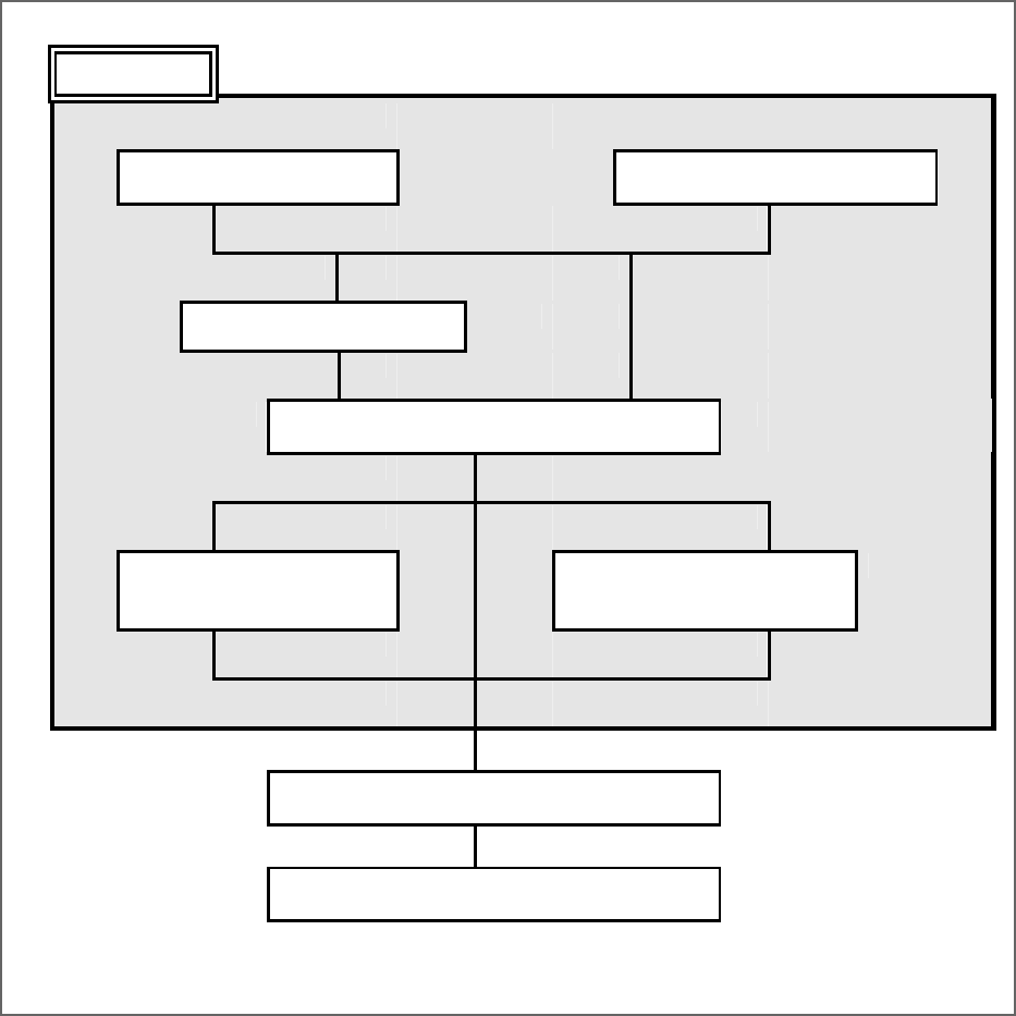
MIL-HDBK-17-1F

Volume 1, Chapter 1 Objectives

1-2

MIL-HDBK-17

MATRIX MATERIAL

CHARACTERIZATION

FIBER CHARACTERIZATION

PREPREG EVALUATION

LAMINA/LAMINATE

CHARACTERIZATION

NOTCHED/DAMAGED

LAMINATE

EVALUATION

JOINT

EVALUATION

DETERMINATION OF

STRUCTURAL DESIGN VALUES

CERTIFICATION OF THE

COMPOSITE STRUCTURE

FIGURE 1.1 Focus of MIL-HDBK-17 indicated by shaded block.

• Volume 2: Provides a repository of potential design data. The documented property summaries

for material systems provide data meeting the criteria for any of the MIL-HDBK-17 data classes.

• Volume 3: Source for additional technical guidance on a wide variety of disciplines related to

polymer matrix composites.

1.3 SCOPE

For Department of Defense purposes, this handbook is for guidance only. This handbook cannot be

cited as a requirement. If it is, the contractor does not have to comply. This mandate is a DoD require-

ment only; it is not applicable to the Federal Aviation Administration (FAA) or other government agencies.

The three volumes of MIL-HDBK-17 serve as a general reference source for technical information on

polymer matrix composites, including:

MIL-HDBK-17-1F

Volume 1, Chapter 1 Objectives

1-3

1.3.1 Strength properties and allowables data

Statistically-based strength property data are defined for each composite material system over a

range of potential usage conditions. The intent is to provide data at the upper and lower limits of the po-

tential environmental conditions for a particular material, so that application issues do not govern the me-

chanical property characterizations. If data are also available at intermediate environmental conditions,

they are used to more exactly define the relationship between the mechanical properties and the effect of

the environment on those properties.

The statistically-based strength data that are available are tabulated in Volume 2. These data are

useful as a starting point for establishing structural design allowables when stress and strength analysis

capabilities permit lamina level margin of safety checks. Where such cases exist, the MIL-HDBK-17 sta-

tistically reduced strength data may be used in determining material design allowables. Depending on the

application, some structural design allowables will have to be determined empirically by laminate, ele-

ment, or higher level of testing, since MIL-HDBK-17 does not provide these data.

Additional information and properties are added as they become available and are demonstrated to

meet the guideline criteria. Typical property values, as well as S-values (see definitions) are included if

they meet the approval of the MIL-HDBK-17 Coordination Group.

When the guidelines or data requirements of MIL-HDBK-17 cannot be followed, the certifying or pro-

curing government agency should be contacted to determine data requirements and other documentation

which may be necessary to justify data values proposed or used by the manufacturer.

1.3.2 Volume 1: Guidelines for Characterization of Structural Materials

This volume contains guidelines for determining the properties of composite material systems, their

constituents, and generic structural elements, including test planning, test matrices, sampling, condition-

ing, test procedure selection, data reporting, data reduction, statistical analysis, and other related topics.

Special attention is given to the statistical treatment and analysis of data. Volume 1 contains guidelines

for general development of material characterization data as well as specific requirements for publication

of material data in MIL-HDBK-17.

It must be emphasized that this handbook differentiates between material basis values (material al-

lowables) and design allowable values. Material basis values, being an intrinsic property of a composite

material system, are the focus of this handbook. Design allowable values, while often rooted in material

basis values, are application dependent, and consider and include specific additional considerations that

may further affect the strength or stiffness of the structure. Also, when establishing application design

values there may be additional certification or procurement agency requirements that go beyond

MIL-HDBK-17.

1.3.3 Volume 2: Material Properties

Volume 2 contains statistically-based data meeting specific MIL-HDBK-17 population sampling and

data documentation requirements, covering constituents and material systems of general interest. Data

published in Volume 2 are under the jurisdiction of the Data Review Working Group and are approved by

the overall Coordination Group (The MIL-HDBK-17 Coordination Group and Working Groups are dis-

cussed in Section 1.5). New material systems will be included and additional material data for existing

systems will be added as data becomes available and are approved. Selected historical data from the

MIL-HDBK-17A version of the handbook that do not meet current data sampling, test methodology, or

documentation requirements, but that still are of potential interest to the industry, are also documented in

an appendix to this volume.

The material properties in Volume 2 are defined over a range of potential use conditions, focusing,

when possible, on the upper and lower material environmental limits so that application-specific environ-

MIL-HDBK-17-1F

Volume 1, Chapter 1 Objectives

1-4

ments do not limit use of the data. Data at intermediate environmental conditions, when available, pro-

vide additional definition of the relation between material response and environment.

While the process of establishing structural design values for specific applications can begin with the

data contained in Volume 2, most applications require collection of additional data, especially if there are

requirements for data from the laminate or higher structural complexity levels (structural complexity level

is discussed in 2.1.2.1). Also, the ability to manufacture material equivalent to that from which the data in

Volume 2 were obtained typically must be proven to the procuring or certifying agency, which usually in-

volves limited testing and data comparison. General guidelines for such material/process equivalence

evaluation are presented in Volume 1; however, many of the details of such an evaluation remain at the

discretion of the procuring or certifying agency.

1.3.4 Volume 3: Materials Usage, Design, and Analysis Guidelines

Volume 3 provides methodologies and lessons learned for the design, manufacture, analysis, and

supportability of composite structures, and for utilization of the material data provided in Volume 2 consis-

tent with the guidance provided in Volume 1. Topics discussed in Volume 3 include materials and proc-

essing, quality control, design and analysis, joints, reliability, thick composites, and supportability.

1.4 USE OF THE DOCUMENT AND LIMITATIONS

1.4.1 Roadmaps for use of Volumes 1 - 3

The following pages provide summary roadmaps that are intended to be brief guides to relevant sec-

tions of this document pertaining to the following topics. The roadmaps are brief guides to the handbook,

and while they indicate a general process flow for the topics, they do not show the detailed process flows,

interactions and loops that are required in the actual process implementation. In some cases there are

overlaps between the various roadmaps. Some minor sections have not been included; for these the

reader is referred to the complete handbook table of contents.

Roadmap #1: Use of New Material in Design and Structural Substantiation

This roadmap covers the qualification of a new material, development of material allowables and struc-

tural design values, and designing, analyzing and certifying a structure with the new material. This road-

map would be typically used by a design organization.

Roadmap #2: Qualification of New Material

This roadmap covers the process for qualifying a new material and establishing the corresponding mate-

rial procurement specification. This roadmap would be typically used by an design organization.

Roadmap #3: Development of Lamina Allowables

This roadmap covers the process for developing lamina level material allowables for a material. This

roadmap could be used by a material supplier who wishes to provide allowables to customers or by a de-

sign organization.

Roadmap #4: Development of Data for New Material for Submittal to Volume 2

This roadmap covers the process for developing material data for submittal to the Handbook for the calcu-

lation of material properties and allowables, and subsequent publication in Volume 2. This roadmap could

be used by a material supplier or by a design organization.

MIL-HDBK-17-1F

Volume 1, Chapter 1 Objectives

1-5

Roadmap #5: Use of Volume 2 Data for Design and Structural Substantiation

This roadmap covers the process for obtaining Volume 2 data, and for performing "equivalency" testing to

validate use of the material in the manufacturer's fabrication process.

Roadmap #6: Demonstration of Equivalency for Revised Material and/or Process

This roadmap covers the process for demonstrating the "equivalency" of a minor change to a material or

to a part fabrication process. This roadmap could be used by a material supplier or by a design organiza-

tion.

Roadmap #7: Demonstration of Application Acceptance for "2

Source" Material

This roadmap covers the process for demonstrating the acceptability of substituting a new material for the

original material used to design and certify a part. "New" material refers to a different fiber or resin mate-

rial, or to a major change to the original material. This roadmap would be typically used by an design or-

ganization.

Roadmap #8: Bolted Joint Tests and Analysis Methods

This roadmap covers development of allowables and design values for, and the design and analysis of

bolted joints.

Roadmap #9: Bonded Joint Tests and Analysis Methods

This roadmap covers development of allowables and design values for, and the design and analysis of

bonded joints.

Roadmap #10: Design, Analysis and Fabrication of Repairs

This roadmap covers development of allowables and design values for, the design and analysis, and the

fabrication of repairs to composite laminates.

MIL-HDBK-17-1F

Volume 1, Chapter 1 Objectives

1-6

Roadmap #1: Use of New Material in Design and Structural Substantiation

Qualify Material (see Roadmap #2)

Develop Lamina Allowables (see Roadmap #3)

Review Building Block Approach

(Volume 3, Chapter 4)

Develop Laminate Allowables

Unnotched Tension, Compression, Shear

(Volume 1, Chapter 6)

(process similar to Roadmap #3)

Develop Structural Design Data

Fracture Toughness (Volume 1, Section 6.8.6)

Strength after Impact (Volume 1, Section 6.10, 7.7)

Notched Tension, Compression (Volume 1, Section 7.4)

Bolted Joints (Volume 1, Section 7.5)

Bonded Joints (Volume 1, Section 7.6)

Fatigue (V1, Sec. 2.5.14, 6.8, V3, Chapter 7)

Damage Tolerance (Volume 3, Chapter 7)

Design and Analyze Structure

Laminate Strength

(Volume 3, Chapter 5.4)

Compression Buckling/Crippling (Volume 3, Section 5.7)

Bonded Joints (Volume 3, Section 6.2)

Bolted Joints (Volume 3, Section 6.3)

Fatigue (Volume 3, Chapter 7)

Damage Tolerance (Volume 3, Chapter 7)

Repairs (Volume 3, Chapter 8)

Thick Section Composites (Volume 3, Chapter 10)

Lessons Learned (Volume 3, Chapter 12)

Establish Design Criteria and Certification

Approach for Specific Application

MIL-HDBK-17-1F

Volume 1, Chapter 1 Objectives

1-7

Roadmap #2: Qualification of New Material

Develop Material and Process Specifications

Volume 3, Chapter 2 (overview)

Volume 3, Section 2.11 (specifics)

Define Test Matrix

Volume 1, Section 2.3.2, 2.3.3

Define Test Methods

Volume 1, Chapters 3 - 6

Purchase Material (multiple batches)

Perform Tests

Reduce/Normalize Test Data

Volume 1, Section 2.4

Calculate Acceptance Limits for Material Specification

Volume 1, Section 8.4.2

Develop QA/QC Procedures, Acceptance Tests for Material

Volume 1, Section 2.3.3, 8.4.2

Volume 3, Section 2.11

Volume 3, Chapter 3

MIL-HDBK-17-1F

Volume 1, Chapter 1 Objectives

1-8

Roadmap #3: Development of Lamina Allowables

Develop Material and Process Specifications

Volume 3, Section 2.11

Define Test Matrix

Volume 1, Section 2.2 (planning)

Volume 1, Section 2.3.2, 8.2 (matrix)

Define Test Methods

Volume 1, Chapters 3 - 6

Purchase Material (multiple batches)

Perform Tests

Certification Agency witnessing as required

Reduce/Normalize Test Data

Volume 1, Section 2.4

Calculate Allowables

Volume 1, Section 8.3.1 - 8.3.4

(individual allowables calculation for each environment)

Volume 1, Section 8.3.5

(allowables by regression versus layup parameter)

Volume 1, Section 8.tbd

(allowables calculation for pooled data across environments)

Develop QA/QC Procedures, Acceptance Tests for Material

Volume 1, Section 2.3.3, 8.4.2

Volume 3, Section 2.11

Volume 3, Chapter 3

MIL-HDBK-17-1F

Volume 1, Chapter 1 Objectives

1-9

Roadmap #4: Development of Data for New Material for Submittal to Volume 2

Develop Material and Process Specifications

Volume 3, Section 2.11

(boilerplate spec if being done by material supplier)

Define Test Matrix

Volume 1, Section 2.2 (planning)

Volume 1, Section 2.3.2, 8.2 (matrix)

Volume 1, Section 2.5 (data submittal)

Define Test Methods

Volume 1, Chapters 3 - 7

Perform Tests

Certification Agency witnessing as required

Collect all required data

Validate data

Reduce and Document Test Data

Volume 1, Sections 2.4 - 2.5

Submit Data to Mil-Hdbk-17 Secretariat

Develop QA/QC Procedures, Acceptance Tests for Material

Volume 1, Section 2.3.3, 8.4.2

Volume 3, Section 2.11

Volume 3, Chapter 3

Review Procedures for Data Documentation and Submittal

Volume 1, Section 2.5

See also www.mil17.org

MIL-HDBK-17-1F

Volume 1, Chapter 1 Objectives

1-10

Roadmap #5: Use of Volume 2 Data for Design and Structural Substantiation

Develop Material and Process Specifications

Volume 3, Section 2.11

Define Equivalency Test Matrix and Success Criteria

Volume 1, Section 2.2 (planning)

Volume 1, Section 2.3.7, 8.2 (matrix)

Define Test Methods

Volume 1, Chapters 3 - 7

Perform Tests

Certification Agency witnessing as required

Reduce/Normalize Test Data

Volume 1, Section 2.4

Perform Statistical Tests

Volume 1, Section 8.4.3

Develop QA/QC Procedures, Acceptance Tests for Material

Volume 1, Section 2.3.3, 8.4.2

Volume 3, Section 2.11, Chapter 3

Obtain Volume 2 data for original material data source.

Obtain material procurement and processing infomation

corresponding to data in Volume 2.

Assess differences between original data source layup and cure

process and "new" manufacturer's processes

All Data

Pass?

Retests for Data

that do not pass

Statistical Tests

Volume 1, tbd

Use Volume 2

data

YesNo

Perform additional environment and higher scale structural tests

MIL-HDBK-17-1F

Volume 1, Chapter 1 Objectives

1-11

Roadmap #6: Demonstration of Equivalency for Revised Material and/or Process

Define Equivalency Test Matrix and Success Criteria

Volume 1, Section 2.2 (planning)

Volume 1, Section 2.3.4.2, 8.2 (matrix)

Define Test Methods

Volume 1, Chapters 3 - 7

Perform Tests

Certification Agency witnessing as required

Reduce/Normalize Test Data

Volume 1, Section 2.4

Perform Statistical Tests

Volume 1, Section 8.4.3

Assess differences between "original" material and/or process

and "new" material and/or process

Volume 1, Section 2.3.4.2

All Data

Pass?

Retests for Data

that do not pass

Statistical Tests

Volume 1, tbd

Accept change in

material or

process

YesNo

Perform additional environment and higher scale structural tests

as required

MIL-HDBK-17-1F

Volume 1, Chapter 1 Objectives

1-12

Roadmap #7: Demonstration of Application Acceptance for "2

Source" Material

Define Equivalency Test Matrix and Success Criteria

Volume 1, Section 2.2 (planning)

Volume 1, Section 2.3.4.1, 8.2 (matrix)

Define Test Methods

Volume 1, Chapters 3 - 7

Perform Tests

Certification Agency witnessing as required

Reduce/Normalize Test Data

Volume 1, Section 2.4

Perform Statistical Tests

Volume 1, Section 8.tbd

Assess differences between "original" material and

"new" material

Volume 1, Section 2.3.4.1

All Data

Pass?

Retests for Data

that do not pass

Statistical Tests

Volume 1, tbd

Accept new

material

YesNo

Perform additional environment and higher scale structural tests

as required to demonstrate acceptability of new material in

specific structural application

MIL-HDBK-17-1F

Volume 1, Chapter 1 Objectives

1-13

Roadmap #8: Bolted Joint Tests and Analysis Methods

Develop Test Matrix

Volume 1, Section 7.4.4, 7.5.3.3, 7.5.4, 7.5.6 (laminate strength)

Volume 1, Section 7.5.7 (fastener strength)

Reduce/Normalize Test Data

Volume 1, Section 2.4

Calculate Allowables and Design Values

Volume 1, Section 8.3

Analysis Methods

Volume 3, Section 6.3

Volume 3, Section 8.3.4.3 (bolted repairs)

Lessons Learned

Volume 3, Section 12.2.6.1, 12.3.1

MIL-HDBK-17-1F

Volume 1, Chapter 1 Objectives

1-14

Roadmap #9: Bonded Joint Tests and Analysis Methods

Develop Test Matrix

Volume 1, Section 7.6.2

Volume 1, Section 6.7.8

Calculate Allowables and Design Values

Volume 1, Section 8.3

Analysis Methods

Volume 3, Section 6.2 (Bonded Joints)

Volume 3, Section 7.7.4.2 (Disbond Growth)

Volume 3, Section 7.8.4.2 (Disbonds)

Volume 3, Section 8.3.4.4 (Bonded Repairs)

Lessons Learned

Volume 3, Section 12.2.6.2, 12.3.1.3

Reference Sections

Volume 1, Chapter 4

Volume 3, Chapter 2

Develop Material and Process Specifications

Volume 3, Section 2.11

MIL-HDBK-17-1F

Volume 1, Chapter 1 Objectives

1-15

Roadmap #10: Design, Analysis and Fabrication of Repairs

Bonded Repair Analysis Methods

Volume 3, Chapter 5

Volume 3, Section 6.2 (Bonded Joints)

Volume 3, Section 7.7.4.2 (Disbond Growth)

Volume 3, Section 7.8.4.2 (Disbonds)

Volume 3, Section 8.3.4.4 (Bonded Repairs)

Lessons Learned

Volume 3, Chapter 12

Characterize Repair Materials

Develop Material and Process Specifications, Volume 3, Section 2.11

Develop Lamina Allowables (see Roadmap #3)

Develop Laminate Allowables (similar to Roadmap #3)

Develop Bolted Joint Allowables, Volume 1, Sections 7.4 - 7.5

Develop Adhesive Allowables, Volume 1, Section 7.6.2

Develop Bonded Joint Allowables, Volume 1, Section 7.6.3

Calculate Allowables and Design Values, Volume 1, Section 8.3

Bolted Repair Analysis Methods

Volume 3, Chapter 5

Volume 3, Section 6.3

Volume 3, Section 8.3.4.3 (Bolted Repairs)

Design for Repair

Volume 3, Section 8.2

Repair Design

Volume 3, Section 8.3

MIL-HDBK-17-1F

Volume 1, Chapter 1 Objectives

1-16

1.4.2 Source of information

The information contained in MIL-HDBK-17 is obtained from materials producers and fabricators, the

aerospace industry, reports on government-sponsored research, the open literature, direct contacts with

researchers, and from participants in MIL-HDBK-17 coordination activities. All information published in

this document has been coordinated and reviewed by representatives from industry, the US Army, the US

Navy, the US Air Force, NASA, and the US Federal Aviation Administration. Every effort has been made

to reflect the most up-to-date information on the use of composite materials, with particular emphasis on

use of composites in structures. The handbook is continually reviewed and revised to keep current with

the state-of-the-art and insure completeness and accuracy.

1.4.3 Use of data and guidelines in applications

All data contained herein are based on small-scale test specimens for specific environmental condi-

tions, largely limited to uniaxial quasi-static loading.

It is the user's responsibility to determine if hand-

book data is appropriate for a given application, and if selected, to translate or scale the data as neces-

sary for use:

• in a multi-directional laminate,

• on a structure of different characteristic size and geometry,

• under a multi-directional stress state,

• when exposed to a different environment, and/or

• when subjected to non-static loading.

Further discussions of these and other issues are provided in Volume 3. Specific uses of handbook data

are beyond the scope and responsibility of MIL-HDBK-17, and applicability and interpretation of specific

provisions of this handbook may require approval by an appropriate procurement or certification agency.

1.4.4 Strength properties and allowables terminology

The handbook intent is to provide guidelines for generating material property data, including statisti-

cally-based strength data at environmental extremes that bracket most intermediate application-specific

environments. The philosophy is to avoid having application-specific issues govern generic material

property characterization programs. If data are also available at intermediate environmental conditions,

they can be used to more completely define the relationship between the property and the effect of the

environment on that property. However, in some cases an environmental limit for a composite material

system may be application dependent, and in others, data at environmental limits may not be available.

Available statistically-based strength data are tabulated in Volume 2. These data are useful as a

starting point for establishing structural design allowable values when stress and strength analysis capa-

bilities permit lamina-level margin-of-safety calculations. For such cases the MIL-HDBK-17 strength basis

value may also be termed a material design allowable. Depending on the application, some structural

design allowables may have to be empirically determined from additional laminate, element, or higher-

level test data not provided by MIL-HDBK-17.

1.4.5 Use of references

While many references are provided at the end of each chapter, note that the information in these

citations may not necessarily comply in every respect either with the general guidelines for data develop-

ment or with the specific requirements for publication of data in the handbook. The references are simply

Unless otherwise noted, tests were conducted in conformance with the particular test method noted. The emphasis is on data ob-

tained from ASTM standard test methods for advanced composites, but where an ASTM test method has been deemed inappropri-

ate or is not yet available, or when data from a nonstandard but commonly practiced test procedure is available, then data from a

non-standard test method may have been accepted for publication. The specific test method used is noted in the data documenta-

tion. See also the statement on test method acceptance criteria in Section 2.5.5.

MIL-HDBK-17-1F

Volume 1, Chapter 1 Objectives

1-17

intended to be helpful, but not necessarily complete or authoritative sources of additional related informa-

tion on specific subject areas.

1.4.6 Use of tradenames and product names

Use of tradenames or proprietary product names does not constitute an endorsement of those prod-

ucts by the US Government or by the MIL-HDBK-17 Coordination Group.

1.4.7 Toxicity, health hazards, and safety

Certain processing and test methods discussed in MIL-HDBK-17 may involve hazardous materials,

operations, or equipment. These methods may not address safety problems, if any, associated with their

use. It is the responsibility of the user of these methods to establish appropriate safety and health prac-

tices and to determine the applicability of regulatory limitations prior to use. The user is referred to the

Advanced Composite Materials US Army Interim Health and Safety Guidance for a discussion of the

health and safety issues involved in the processing and use of composite materials. This document is

generated by the US Army Environmental Hygiene Agency, Aberdeen Proving Ground, MD. Material

manufacturers, as well as various composites user groups, may also provide guidance on health and

safety issues pertinent to composite materials.

1.4.8 Ozone depleting chemicals

Restrictions on the use of ozone depleting chemicals are detailed in the US Clean Air Act of 1991.

1.5 APPROVAL PROCEDURES

The content of the handbook is developed and approved by the MIL-HDBK-17 Coordination Group,

which meets twice yearly to consider changes and additions to the handbook. This Group consists of the

handbook Co-Chairs, Coordinator, Secretariat, Working Group Chairs, and the active Working Group par-

ticipants, which include representatives from various US and international procuring and certifying agen-

cies, in addition to the producing industries and academic and research institutions. MIL-HDBK-17 Coor-

dination Group meetings are announced to participants by mail about eight weeks prior to the scheduled

meeting date, and minutes of the meetings are mailed eight weeks following the close of the meeting.

While each of the Working Groups functions similarly, they are of three types: Executive, a single

Working Group with oversight responsibility composed of the Working Group Chairs, the handbook Co-

Chairs, Coordinator, and Secretariat; Standing, including Data Review, Guidelines, Materials and Proc-

essing, Statistics, and Testing Working Groups; and Specialty, which varies with time but currently in-

cludes the Braiding and Filament Winding, Supportability, Structural Joints, and Thick-Sections Working

Groups. The makeup and organization of the Coordination Group and Working Groups, as well as the

procedures followed for document change approval, are summarized in the MIL-HDBK-17 Coordination

Group Member's Guide, separately published and available from either the Coordinator or Secretariat.

Proposals for addition to, deletion from, or modification to the handbook should be submitted to both

the appropriate Working Group and the Secretariat well in advance of the announcement mailing date,

and should include specific notation of the proposed changes and adequate documentation of supporting

data or analytical procedures. Reproducible copies of figures, drawings, or photographs proposed for

publication in the document should be furnished to the Secretariat. Following approval by the appropriate

Working Group, the proposed changes are published in the next minutes of the Coordination Group, in a

special section of the minutes called the "yellow pages", and all participants are allowed comment on the

proposed changes. If no substantive comments are received on any individual item by the posted re-

sponse date, then that item is considered approved by the Coordination Group and is considered effective

as of that date. (Prior to publication in the next revision of the handbook the collected changes are re-

viewed by various branches of the US DOD. Additional proposals for revision may result from this US

DOD review.)

MIL-HDBK-17-1F

Volume 1, Chapter 1 Objectives

1-18

Requests for inclusion of material property data into MIL-HDBK-17 should be submitted to either the

Coordinator or the Secretariat, accompanied by the documentation specified in Section 2.5.5. A Data

Source Information Package has been created to aid those considering submitting data for inclusion in

MIL-HDBK-17, and is available from either the Coordinator or the Secretariat. The Secretariat reviews

and analyzes each data submission and at the next available meeting of the Coordination Group presents

a summary for evaluation by the Data Review Working Group. The choice of new materials to be in-

cluded herein is governed by the MIL-HDBK-17 Coordination Group. Practical considerations preclude

inclusion of all advanced composite materials, but reasonable attempts will be made to add new material

systems of interest in a timely manner.

1.6 SYMBOLS, ABBREVIATIONS, AND SYSTEMS OF UNITS

This section defines the symbols and abbreviations which are used within MIL-HDBK-17 and de-

scribes the system of units which is maintained. Common usage is maintained where possible. Refer-

ences 1.6(a), 1.6(b), and 1.6(c) served as primary sources for this information.

1.6.1 Symbols and abbreviations

The symbols and abbreviations used in this document are defined in this section with the exception of

statistical symbols. These latter symbols are defined in Chapter 8. The lamina/laminate coordinate axes

used for all properties and a summary of the mechanical property notation are shown in Figure 1.6.1.

• The symbols f and m, when used as either subscripts or superscripts, always denote fiber and

matrix, respectively.

• The type of stress (for example, cy - compression yield) is always used in the superscript position.

• Direction indicators (for example, x, y, z, 1, 2, 3, etc.) are always used in the subscript position.

• Ordinal indicators of laminae sequence (e.g., 1, 2, 3, etc.) are used in the superscript position and

must be parenthesized to distinguish them from mathematical exponents.

• Other indicators may be used in either subscript or superscript position, as appropriate for clarity.

• Compound symbols (such as, basic symbols plus indicators) which deviate from these rules are

shown in their specific form in the following list.

The following general symbols and abbreviations are considered standard for use in MIL-HDBK-17.

Where exceptions are made, they are noted in the text and tables.

A - (1) area (m

,in

)

- (2) ratio of alternating stress to mean stress

- (3) A-basis for mechanical property values

a - (1) length dimension (mm,in)

- (2) acceleration (m/sec

,ft/sec

)

- (3) amplitude

- (4) crack or flaw dimension (mm,in)

B - (1) B-basis for mechanical property values

- (2) biaxial ratio

Btu - British thermal unit(s)

b - width dimension (mm,in), e.g., the width of a bearing or compression panel normal to load,

or breadth of beam cross-section

MIL-HDBK-17-1F

Volume 1, Chapter 1 Objectives

1-19

FIGURE 1.6.1 Mechanical property notation.

MIL-HDBK-17-1F

Volume 1, Chapter 1 Objectives

1-20

C - (1) specific heat (kJ/kg °C,Btu/lb °F)

- (2) Celsius

CF - centrifugal force (N,lbf)

CPF - crossply factor

CPT - cured ply thickness (mm, in.)

CG - (1) center of mass, "center of gravity"

- (2) area or volume centroid

- centerline

c - column buckling end-fixity coefficient

- honeycomb sandwich core depth (mm,in)

cpm - cycles per minute

D - (1) diameter (mm,in)

- (2) hole or fastener diameter (mm,in)

- (3) plate stiffness (N-m,lbf-in)

d - mathematical operator denoting differential

E - modulus of elasticity in tension, average ratio of stress to strain for stress below propor-

tional limit (GPa,Msi)

E' - storage modulus (GPa,Msi)

E" - loss modulus (GPa,Msi)

- modulus of elasticity in compression, average ratio of stress to strain for stress below

proportional limit (GPa,Msi)

’

- modulus of elasticity of honeycomb core normal to sandwich plane (GPa,Msi)

sec

- secant modulus (GPa,Msi)

tan

- tangent modulus (GPa,Msi)

e - minimum distance from a hole center to the edge of the sheet (mm,in)

e/D - ratio of edge distance to hole diameter (bearing strength)

F - (1) stress (MPa,ksi)

- (2) Fahrenheit

- bending stress (MPa,ksi)

ccr

- crushing or crippling stress (upper limit of column stress for failure) (MPa,ksi)

- ultimate stress in pure shear (this value represents the average shear stress over the

cross-section) (MPa,ksi)

FAW - fiber areal weight (g/m

, lb/in

)

FV - fiber volume (%)

f - (1) internal (or calculated) stress (MPa,ksi)

- (2) stress applied to the gross flawed section (MPa,ksi)

- (3) creep stress (MPa,ksi)

- internal (or calculated) compressive stress (MPa,ksi)

- (1) maximum stress at fracture (MPa,ksi)

- (2) gross stress limit (for screening elastic fracture data (MPa,ksi)

ft - foot, feet

G - modulus of rigidity (shear modulus) (GPa,Msi)

GPa - gigapascal(s)

g - (1) gram(s)

- (2) acceleration due to gravity (m/s

,ft/s

)

H/C - honeycomb (sandwich)

h - height dimension (mm,in) e.g. the height of a beam cross-section

hr - hour(s)

I - area moment of inertia (mm

,in

)

i - slope (due to bending) of neutral plane in a beam, in radians

in. - inch(es)

J - (1) torsion constant (= I

for round tubes) (m

,in

)

- (2) Joule

MIL-HDBK-17-1F

Volume 1, Chapter 1 Objectives

1-21

K - (1) Kelvin

- (2) stress intensity factor (MPa/m,ksi/in)

- (3) coefficient of thermal conductivity (W/m °C, Btu/ft

/hr/in/°F)

- (4) correction factor

- (5) dielectric constant

app

- apparent plane strain fracture toughness or residual strength (MPa/m,ksi/in)

- critical plane strain fracture toughness, a measure of fracture toughness at point of crack

growth instability (MPa/m,ksi/in)

- plane strain fracture toughness (MPa/m,ksi/in)

- empirically calculated fatigue notch factor

- plate or cylinder shear buckling coefficient

- (1) theoretical elastic stress concentration factor

- (2)

/c ratio in H/C sandwich

Kv - dielectric strength (KV/mm, V/mil)

- plate or cylinder compression buckling coefficient

k - strain at unit stress (m/m,in/in)

L - cylinder, beam, or column length (mm,in)

L' - effective column length (mm,in)

lb - pound

M - applied moment or couple (N-m,in-lbf)

Mg - megagram(s)

MPa - megapascal(s)

MS - military standard

M.S. - margin of safety

MW - molecular weight

MWD - molecular weight distribution

m - (1) mass (kg,lb)

- (2) number of half wave lengths

- (3) metre

- (4) slope

N - (1) number of fatigue cycles to failure

- (2) number of laminae in a laminate

- (3) distributed in-plane forces on a panel (lbf/in)

- (4) Newton

- (5) normalized

NA - neutral axis

n - (1) number of times in a set

- (2) number of half or total wavelengths

- (3) number of fatigue cycles endured

P - (1) applied load (N,lbf)

- (2) exposure parameter

- (3) probability

- (4) specific resistance (Ω)

- test ultimate load, (N,lb per fastener)

- test yield load, (N,lb per fastener)

p - normal pressure (Pa,psi)

psi - pounds per square inch

Q - area static moment of a cross-section (mm

,in

)

q - shear flow (N/m,lbf/in)

R - (1) algebraic ratio of minimum load to maximum load in cyclic loading

- (2) reduced ratio

RA - reduction of area

R.H. - relative humidity

RMS - root-mean-square

RT - room temperature

MIL-HDBK-17-1F

Volume 1, Chapter 1 Objectives

1-22

r - (1) radius (mm,in)

- (2) root radius (mm,in)

- (3) reduced ratio (regression analysis)

S - (1) shear force (N,lbf)

- (2) nominal stress in fatigue (MPa,ksi)

- (3) S-basis for mechanical property values

- stress amplitude in fatigue (MPa,ksi)

- fatigue limit (MPa,ksi)

- mean stress in fatigue (MPa,ksi)

max

- highest algebraic value of stress in the stress cycle (MPa,ksi)

min

- lowest algebraic value of stress in the stress cycle (MPa,ksi)

- algebraic difference between the minimum and maximum stresses in one cycle (MPa,ksi)

S.F. - safety factor

s - (1) arc length (mm,in)

- (2) H/C sandwich cell size (mm,in)

T - (1) temperature (°C,°F)

- (2) applied torsional moment (N-m,in-lbf)

- thermal decomposition temperature (°C,°F)

- exposure temperature (°C,°F)

- glass transition temperature (°C,°F)

- melting temperature (°C,°F)

t - (1) thickness (mm,in)

- (2) exposure time (s)

- (3) elapsed time (s)

V - (1) volume (mm

,in

)

- (2) shear force (N,lbf)

W - (1) weight (N,lbf)

- (2) width (mm,in)

- (3) Watt

x - distance along a coordinate axis

Y - nondimensional factor relating component geometry and flaw size

y - (1) deflection (due to bending) of elastic curve of a beam (mm,in)

- (2) distance from neutral axis to given point

- (3) distance along a coordinate axis

Z - section modulus, I/y (mm

,in

)

- coefficient of thermal expansion (m/m/°C,in/in/°F)

- shear strain (m/m,in/in)

∆

- difference (used as prefix to quantitative symbols)

- elongation or deflection (mm,in)

- strain (m/m,in/in)

- elastic strain (m/m,in/in)

- plastic strain (m/m,in/in)

- permeability

- plasticity reduction factor

[η] - intrinsic viscosity

* - dynamic complex viscosity

- Poisson's ratio

- (1) density (kg/m3,lb/in3)

- (2) radius of gyration (mm,in)

’

- H/C sandwich core density (kg/m

,lb/in

)

- total, summation

- standard deviation

- stress in j direction on surface whose outer normal is in i direction (i, j = 1, 2, 3 or x, y, z)

(MPa,ksi)

MIL-HDBK-17-1F

Volume 1, Chapter 1 Objectives

1-23

- applied shear stress (MPa,ksi)

- angular velocity (radians/s)

∞

- infinity

1.6.1.1 Constituent properties

The following symbols apply specifically to the constituent properties of a typical composite material.

- Young's modulus of filament material (MPa,ksi)

- Young's modulus of matrix material (MPa,ksi)

- Young's modulus of impregnated glass scrim cloth in the filament direction or in the warp di-

rection of a fabric (MPa,ksi)

- Young's modulus of impregnated glass scrim cloth transverse to the filament direction or to the

warp direction in a fabric (MPa,ksi)

- shear modulus of filament material (MPa,ksi)

- shear modulus of matrix (MPa,ksi)

- shear modulus of impregnated glass scrim cloth (MPa,ksi)

’

- shear modulus of sandwich core along X-axis (MPa,ksi)

’

- shear modulus of sandwich core along Y-axis (MPa,ksi)



- filament length (mm,in)

- coefficient of thermal expansion for filament material (m/m/°C,in/in/°F)

- coefficient of thermal expansion for matrix material (m/m/°C,in/in/°F)

- coefficient of thermal expansion of impregnated glass scrim cloth in the filament direction or in

the warp direction of a fabric (m/m/°C,in/in/°F)

- coefficient of thermal expansion of impregnated glass scrim cloth transverse to the filament di-

rection or to the warp direction in a fabric (m/m/°C,in/in/°F)

- Poisson's ratio of filament material

- Poisson's ratio of matrix material

- glass scrim cloth Poisson's ratio relating to contraction in the transverse (or fill) direction as a

result of extension in the longitudinal (or warp) direction

- glass scrim cloth Poisson's ratio relating to contraction in the longitudinal (or warp) direction

as a result of extension in the transverse (or fill) direction

- applied axial stress at a point, as used in micromechanics analysis (MPa,ksi)

- applied shear stress at a point, as used in micromechanics analysis (MPa,ksi)

1.6.1.2 Laminae and laminates

The following symbols, abbreviations, and notations apply to composite laminae and laminates. At

the present time the focus in MIL-HDBK-17 is on laminae properties. However, commonly used nomen-

clature for both laminae and laminates are included here to avoid potential confusion.

(i,j = 1,2,6) - extensional rigidities (N/m,lbf/in)

(i,j = 1,2,6) - coupling matrix (N,lbf)

(i,j = 1,2,6) - elements of stiffness matrix (Pa,psi)

, D

- flexural rigidities (N-m,lbf-in)

- twisting rigidity (N-m,lbf-in)

(i,j = 1,2,6) - flexural rigidities (N-m,lbf-in)

- Young's modulus of lamina parallel to filament or warp direction (GPa,Msi)

- Young's modulus of lamina transverse to filament or warp direction (GPa,Msi)

- Young's modulus of laminate along x reference axis (GPa,Msi)

MIL-HDBK-17-1F

Volume 1, Chapter 1 Objectives

1-24

- Young's modulus of laminate along y reference axis (GPa,Msi)

- shear modulus of lamina in 12 plane (GPa,Msi)

- shear modulus of laminate in xy reference plane (GPa,Msi)

- thickness of i

ply or lamina (mm,in)

, M

- bending and twisting moment components (N-m/m, in-lbf/in in plate and shell analy-

sis)

- number of filaments per unit length per lamina

, Q

- shear force parallel to z axis of sections of a plate perpendicular to x and y axes, re-

spectively (N/m,lbf/in)

(i,j = 1,2,6) - reduced stiffness matrix (Pa,psi)

, u

- components of the displacement vector (mm,in)

- components of the displacement vector at the laminate's midsurface (mm,in)

- void content (% by volume)

- filament content or fiber volume (% by volume)

- glass scrim cloth content (% by volume)

- matrix content (% by volume)

, V

- edge or support shear force (N/m,lbf/in)

- filament content (% by weight)

- glass scrim cloth content (% by weight)

- matrix content (% by weight)

- weight of laminate per unit surface area (N/m

,lbf/in

)

- lamina coefficient of thermal expansion along 1 axis (m/m/°C,in/in/°F)

- lamina coefficient of thermal expansion along 2 axis (m/m/°C,in/in/°F)

- laminate coefficient of thermal expansion along general reference x axis (m/m/°C,

in/in/°F)

- laminate coefficient of thermal expansion along general reference y axis (m/m/°C,

in/in/°F)

- laminate shear distortion coefficient of thermal expansion (m/m/°C,in/in/°F)

- angular orientation of a lamina in a laminate, i.e., angle between 1 and x axes (°)

- product of

and

- Poisson's ratio relating contraction in the 2 direction as a result of extension in the 1

direction

- Poisson's ratio relating contraction in the 1 direction as a result of extension in the 2

direction

- Poisson's ratio relating contraction in the y direction as a result of extension in the x

direction

- Poisson's ratio relating contraction in the x direction as a result of extension in the y

direction

- density of a single lamina (kg/m

,lb/in

)

- density of a laminate (kg/m

,lb/in

)

- (1) general angular coordinate, (°)

- (2) angle between

x and load axes in off-axis loading (°)

1.6.1.3 Subscripts

The following subscript notations are considered standard in MIL-HDBK-17.

1, 2, 3 - laminae natural orthogonal coordinates (1 is filament or warp direction)

A - axial

a - (1) adhesive

- (2) alternating

app - apparent

The convention for Poisson’s ratio should be checked before comparing different sources as different conventions are used.

MIL-HDBK-17-1F

Volume 1, Chapter 1 Objectives

1-25

byp - bypass

c - composite system, specific filament/matrix composition. Composite as a whole, contrasted

to individual constituents. Also, sandwich core when used in conjunction with prime (')

- (4) critical

cf - centrifugal force

e - fatigue or endurance

eff - effective

eq - equivalent

f - filament

g - glass scrim cloth

H - hoop

i - i

position in a sequence

L - lateral

m - (1) matrix

- (2) mean

max - maximum

min - minimum

n - (1) n

(last) position in a sequence

- (2) normal

p - polar

s - symmetric

st - stiffener

T - transverse

t - value of parameter at time t

x, y, z - general coordinate system

∑ - total, or summation

o - initial or reference datum

( ) - format for indicating specific, temperature associated with term in parentheses. RT - room

temperature (21°C,70°F); all other temperatures in °F unless specified.

1.6.1.4 Superscripts

The following superscript notations are considered standard in MIL-HDBK-17.

b - bending

br - bearing

c - (1) compression

- (2) creep

cc - compression crippling

cr - compression buckling

e - elastic

f - filament

g - glass scrim cloth

is - interlaminar shear

(i) - i

ply or lamina

lim - limit, used to indicate limit loading

m - matrix

ohc - open hole compression

oht - open hole tension

p - plastic

pl - proportional limit

rup - rupture

s - shear

scr - shear buckling

sec - secant (modulus)

so - offset shear

MIL-HDBK-17-1F

Volume 1, Chapter 1 Objectives

1-26

T - temperature or thermal

t - tension

tan - tangent (modulus)

u - ultimate

y - yield

' - secondary (modulus), or denotes properties of H/C core when used with subscript c

CAI - compression after impact

1.6.1.5 Acronyms

The following acronyms are used in MIL-HDBK-17.

AA - atomic absorption

AES - Auger electron spectroscopy

AIA - Aerospace Industries Association

ANOVA - analysis of variance

ARL - US Army Research Laboratory

ASTM - American Society for Testing and Materials

BMI - bismaleimide

BVID - barely visible impact damage

CAI - compression after impact

CCA - composite cylinder assemblage

CFRP - carbon fiber reinforced plastic

CLS - crack lap shear

CMCS - Composite Motorcase Subcommittee (JANNAF)

CPT - cured ply thickness

CTA - cold temperature ambient

CTD - cold temperature dry

CTE - coefficient of thermal expansion

CV - coefficient of variation

CVD - chemical vapor deposition

DCB - double cantilever beam

DDA - dynamic dielectric analysis

DLL - design limit load

DMA - dynamic mechanical analysis

DOD - Department of Defense

DSC - differential scanning calorimetry

DTA - differential thermal analysis

DTRC - David Taylor Research Center

ENF - end notched flexure

EOL - end-of-life

ESCA - electron spectroscopy for chemical analysis

ESR - electron spin resonance

ETW - elevated temperature wet

FAA - Federal Aviation Administration

FFF - field flow fractionation

FGRP - fiberglass reinforced plastic

FMECA - Failure Modes Effects Criticality Analysis

FOD - foreign object damage

FTIR - Fourier transform infrared spectroscopy

FWC - finite width correction factor

GC - gas chromatography

GSCS - Generalized Self Consistent Scheme

HDT - heat distortion temperature

HPLC - high performance liquid chromatography

ICAP - inductively coupled plasma emission

MIL-HDBK-17-1F

Volume 1, Chapter 1 Objectives

1-27

IITRI - Illinois Institute of Technology Research Institute

IR - infrared spectroscopy

ISS - ion scattering spectroscopy

JANNAF - Joint Army, Navy, NASA, and Air Force

LC - liquid chromatography

LPT - laminate plate theory

LSS - laminate stacking sequence

MMB - mixed mode bending

MOL - material operational limit

MS - mass spectroscopy

MSDS - material safety data sheet

MTBF - Mean Time Between Failure

NAS - National Aerospace Standard

NASA - National Aeronautics and Space Administration

NDI - nondestructive inspection

NMR - nuclear magnetic resonance

PEEK - polyether ether ketone

RDS - rheological dynamic spectroscopy

RH - relative humidity

RT - room temperature

RTA - room temperature ambient

RTD - room temperature dry

RTM - resin transfer molding

SACMA - Suppliers of Advanced Composite Materials Association

SAE - Society of Automotive Engineers

SANS - small-angle neutron scattering spectroscopy

SEC - size-exclusion chromatography

SEM - scanning electron microscopy

SFC - supercritical fluid chromatography

SI - International System of Units (Le Système International d'Unités)

SIMS - secondary ion mass spectroscopy

TBA - torsional braid analysis

TEM - transmission electron microscopy

TGA - thermogravimetric analysis

TLC - thin-layer chromatography

TMA - thermal mechanical analysis

TOS - thermal oxidative stability

TVM - transverse microcrack

UDC - unidirectional fiber composite

VNB - V-notched beam

XPS - X-ray photoelectron spectroscopy

1.6.2 System of units

To comply with Department of Defense Instructive 5000.2, Part 6, Section M, "Use of the Metric Sys-

tem," dated February 23, 1991, the data in MIL-HDBK-17 are generally presented in both the International

System of Units (SI units) and the U. S. Customary (English) system of units. ASTM E-380, Standard for

Metric Practice, provides guidance for the application for SI units which are intended as a basis for world-

wide standardization of measurement units (Reference 1.6.2(a)). Further guidelines on the use of the SI

system of units and conversion factors are contained in the following publications (References 1.6.2(b) -

(e)):

(1) DARCOM P 706-470, Engineering Design Handbook: Metric Conversion Guide, July 1976.

(2) NBS Special Publication 330, "The International System of Units (SI)," National Bureau of Stan-

dards, 1986 edition.

MIL-HDBK-17-1F

Volume 1, Chapter 1 Objectives

1-28

(3) NBS Letter Circular LC 1035, "Units and Systems of Weights and Measures, Their Origin, Devel-

opment, and Present Status," National Bureau of Standards, November 1985.

(4) NASA Special Publication 7012, "The International System of Units Physical Constants and Con-

version Factors", 1964.

English to SI conversion factors pertinent to MIL-HDBK-17 data are contained in Table 1.6.2.

TABLE 1.6.2 English to SI conversion factors.

___________________________________________________________________________

To convert from to Multiply by

___________________________________________________________________________

Btu (thermochemical)/in

-s watt/meter

(W/m

) 1.634 246 E+06

Btu-in/(s-ft

-°F) W/(m K) 5.192 204 E+02

degree Fahrenheit degree Celsius (°C) T = (T - 32)/1.8

degree Fahrenheit kelvin (K) T = (T + 459.67)/1.8

foot meter (m) 3.048 000 E-01

9.290 304 E-02

foot/second meter/second (m/s) 3.048 000 E-01

ft/s

m/s

3.048 000 E-01

inch meter (m) 2.540 000 E-02

in.

meter

) 6.451 600 E-04

in.

1.638 706 E-05

kilogram-force (kgf) newton (N) 9.806 650 E+00

kgf/m

pascal (Pa) 9.806 650 E+00

kip (1000 lbf) newton (N) 4.448 222 E+03

ksi (kip/in

) MPa 6.894 757 E+00

lbf-in N-m 1.129 848 E-01

lbf-ft N-m 1.355 818 E+00

lbf/in

(psi) pascal (Pa) 6.894 757 E+03

lb/in

gm/m

7.030 696 E+05

lb/in

kg/m

2.767 990 E+04

Msi (10

psi) GPa 6.894 757 E+00

pound-force (lbf) newton (N) 4.488 222 E+00

pound-mass (lb avoirdupois) kilogram (kg) 4.535 924 E-01

torr pascal (Pa) 1.333 22 E+02

___________________________________________________________________________

∗ The letter "E" following the conversion factor stands for exponent and the two

digits after the letter "E" indicate the power of 10 by which the number is to be

multiplied.

MIL-HDBK-17-1F

Volume 1, Chapter 1 Objectives

1-29

1.7 DEFINITIONS

The following definitions are used within MIL-HDBK-17. This glossary of terms is not totally compre-

hensive but it does represent nearly all commonly used terms. Where exceptions are made, they are

noted in the text and tables. For ease of identification the definitions have been organized alphabetically.

A-Basis (or A-Value) -- A statistically-based material property; a 95% lower confidence bound on the

first percentile of a specified population of measurements. Also a 95% lower tolerance bound for the up-

per 99% of a specified population.

A-Stage -- An early stage in the reaction of thermosetting resins in which the material is still soluble

in certain liquids and may be liquid or capable of becoming liquid upon heating. (Sometimes referred to

as resol.)

Absorption -- A process in which one material (the absorbent) takes in or absorbs another (the ab-

sorbate).

Accelerator -- A material which, when mixed with a catalyzed resin, will speed up the chemical reac-

tion between the catalyst and the resin.

Accuracy -- The degree of conformity of a measured or calculated value to some recognized stan-

dard or specified value. Accuracy involves the systematic error of an operation.

Addition Polymerization -- Polymerization by a repeated addition process in which monomers are

linked together to form a polymer without splitting off of water or other simple molecules.

Adhesion -- The state in which two surfaces are held together at an interface by forces or interlock-

ing action or both.

Adhesive -- A substance capable of holding two materials together by surface attachment. In the

handbook, the term is used specifically to designate structural adhesives, those which produce attach-

ments capable of transmitting significant structural loads.

ADK -- Notation used for the k-sample Anderson-Darling statistic, which is used to test the hypothe-

sis that k batches have the same distribution.

Aliquot -- A small, representative portion of a larger sample.

Aging -- The effect, on materials, of exposure to an environment for a period of time; the process of

exposing materials to an environment for an interval of time.

Ambient -- The surrounding environmental conditions such as pressure or temperature.

Anelasticity -- A characteristic exhibited by certain materials in which strain is a function of both

stress and time, such that, while no permanent deformations are involved, a finite time is required to es-

tablish equilibrium between stress and strain in both the loading and unloading directions.

Angleply -- Any balanced laminate consisting of plus and minus theta plies where theta is an acute

angle with respect to a reference direction.

Anisotropic -- Not isotropic; having mechanical and/or physical properties which vary with direction

relative to natural reference axes inherent in the material.

Aramid -- A manufactured fiber in which the fiber-forming substance consisting of a long-chain syn-

thetic aromatic polyamide in which at least 85% of the amide (-CONH-) linkages are attached directly to

two aromatic rings.

MIL-HDBK-17-1F

Volume 1, Chapter 1 Objectives

1-30

Areal Weight of Fiber -- The weight of fiber per unit area of prepreg. This is often expressed as

grams per square meter. See Table 1.6.2 for conversion factors.

Artificial Weathering -- Exposure to laboratory conditions which may be cyclic, involving changes in

temperature, relative humidity, radiant energy and any other elements found in the atmosphere in various

geographical areas.

Aspect Ratio -- In an essentially two-dimensional rectangular structure (e.g., a panel), the ratio of the

long dimension to the short dimension. However, in compression loading, it is sometimes considered to

be the ratio of the load direction dimension to the transverse dimension. Also, in fiber micro-mechanics, it

is referred to as the ratio of length to diameter.

Autoclave -- A closed vessel for producing an environment of fluid pressure, with or without heat, to

an enclosed object which is undergoing a chemical reaction or other operation.

Autoclave Molding -- A process similar to the pressure bag technique. The lay-up is covered by a

pressure bag, and the entire assembly is placed in an autoclave capable of providing heat and pressure

for curing the part. The pressure bag is normally vented to the outside.

Axis of Braiding -- The direction in which the braided form progresses.

B-Basis (or B-Value) -- A statistically-based material property; a 95% lower confidence bound on the

tenth percentile of a specified population of measurements. Also a 95% lower tolerance bound for the

upper 90% of a specified population. (See Volume 1, Section 8.1.4)

B-Stage -- An intermediate stage in the reaction of a thermosetting resin in which the material sof-

tens when heated and swells when in contact with certain liquids but does not entirely fuse or dissolve.

Materials are usually precured to this stage to facilitate handling and processing prior to final cure.

(Sometimes referred to as resitol.)

Bag Molding -- A method of molding or laminating which involves the application of fluid pressure to

a flexible material which transmits the pressure to the material being molded or bonded. Fluid pressure

usually is applied by means of air, steam, water or vacuum.

Balanced Laminate -- A composite laminate in which all identical laminae at angles other than 0 de-

grees and 90 degrees occur only in ± pairs (not necessarily adjacent).

Batch (or Lot) -- For fibers and resins, a quantity of material formed during the same process and

having identical characteristics throughout. For prepregs, laminae, and laminates, material made from

one batch of fiber and one batch of resin.

Bearing Area -- The product of the pin diameter and the specimen thickness.

Bearing Load -- A compressive load on an interface.

Bearing Yield Strength -- The bearing stress at which a material exhibits a specified limiting devia-

tion from the proportionality of bearing stress to bearing strain.

Bend Test -- A test of ductility by bending or folding, usually with steadily applied forces. In some

instances the test may involve blows to a specimen having a cross section that is essentially uniform over

a length several times as great as the largest dimension of the cross section.

Binder -- A bonding resin used to hold strands together in a mat or preform during manufacture of a

molded object.

MIL-HDBK-17-1F

Volume 1, Chapter 1 Objectives

1-31

Binomial Random Variable -- The number of successes in independent trials where the probability

of success is the same for each trial.

Birefringence -- The difference between the two principal refractive indices (of a fiber) or the ratio

between the retardation and thickness of a material at a given point.

Bleeder Cloth -- A nonstructural layer of material used in the manufacture of composite parts to allow

the escape of excess gas and resin during cure. The bleeder cloth is removed after the curing process

and is not part of the final composite.

Bobbin -- A cylinder or slightly tapered barrel, with or without flanges, for holding tows, rovings, or

yarns.

Bond -- The adhesion of one surface to another, with or without the use of an adhesive as a bonding

agent.

Braid -- A system of three or more yarns which are interwoven in such a way that no two yarns are

twisted around each other.

Braid Angle -- The acute angle measured from the axis of braiding.

Braid, Biaxial -- Braided fabric with two-yarn systems, one running in the

+θ direction, the other in

the

-θ direction as measured from the axis of braiding.

Braid Count -- The number of braiding yarn crossings per inch measured along the axis of a braided

fabric.

Braid, Diamond -- Braided fabric with an over one, under one weave pattern, (1 x 1).

Braid, Flat -- A narrow bias woven tape wherein each yarn is continuous and is intertwined with every

other yarn in the system without being intertwined with itself.

Braid, Hercules -- A braided fabric with an over three, under three weave pattern, (3 x 3).

Braid, Jacquard -- A braided design made with the aid of a jacquard machine, which is a shedding

mechanism by means of which a large number of ends may be controlled independently and complicated

patterns produced.

Braid, Regular -- A braided fabric with an over two, under two weave pattern (2 x 2).

Braid, Square -- A braided pattern in which the yarns are formed into a square pattern.

Braid, Two-Dimensional -- Braided fabric with no braiding yarns in the through thickness direction.

Braid, Three-Dimensional -- Braided fabric with one or more braiding yarns in the through thickness

direction.

Braid, Triaxial -- A biaxial braided fabric with laid in yarns running in the axis of braiding.

Braiding -- A textile process where two or more strands, yarns or tapes are intertwined in the bias

direction to form an integrated structure.

Broadgoods -- A term loosely applied to prepreg material greater than about 12 inches in width,

usually furnished by suppliers in continuous rolls. The term is currently used to designate both collimated

uniaxial tape and woven fabric prepregs.

MIL-HDBK-17-1F

Volume 1, Chapter 1 Objectives

1-32

Buckling (Composite) -- A mode of structural response characterized by an out-of-plane material

deflection due to compressive action on the structural element involved. In advanced composites, buck-

ling may take the form not only of conventional general instability and local instability but also a micro-

instability of individual fibers.

Bundle -- A general term for a collection of essentially parallel filaments or fibers.

C-Stage -- The final stage of the curing reaction of a thermosetting resin in which the material has

become practically infusable and insoluble. (Normally considered fully cured and sometimes referred to

as resite.)

Capstan -- A friction type take-up device which moves braided fabric away from the fell. The speed of

which determines the braid angle.

Carbon Fibers -- Fibers produced by the pyrolysis of organic precursor fibers such as rayon, poly-

acrylonitrile (PAN), and pitch in an inert atmosphere. The term is often used interchangeably with "graph-

ite"; however, carbon fibers and graphite fibers differ in the temperature at which the fibers are made and

heat-treated, and the amount of carbon produced. Carbon fibers typically are carbonized at about 2400°F

(1300°C) and assay at 93 to 95% carbon, while graphite fibers are graphitized at 3450 to 5450°F (1900 to

3000°C) and assay at more than 99% elemental carbon.

Carrier -- A mechanism for carrying a package of yarn through the braid weaving motion. A typical

carrier consists of a bobbin spindle, a track follower, and a tensioning device.

Caul Plates -- Smooth metal plates, free of surface defects, the same size and shape as a composite

lay-up, used immediately in contact with the lay-up during the curing process to transmit normal pressure

and to provide a smooth surface on the finished laminate.

Censoring -- Data is right (left) censored at

M, if, whenever an observation is less than or equal to M

(greater than or equal to

M), the actual value of the observation is recorded. If the observation exceeds

(is less than)

M, the observation is recorded as M.

Chain-Growth Polymerization -- One of the two principal polymerization mechanisms. In chain-

growth polymerization, the reactive groups are continuously regenerated during the growth process.

Once started, the polymer molecule grows rapidly by a chain of reactions emanating from a particular re-

active initiator which may be a free radical, cation or anion.

Chromatogram -- A plot of detector response against peak volume of solution (eluate) emerging from

the system for each of the constituents which have been separated.

Circuit -- One complete traverse of the fiber feed mechanism of a winding machine; one complete

traverse of a winding band from one arbitrary point along the winding path to another point on a plane

through the starting point and perpendicular to the axis.

Cocuring -- The act of curing a composite laminate and simultaneously bonding it to some other pre-

pared surface during the same cure cycle (see Secondary Bonding).

Coefficient of Linear Thermal Expansion -- The change in length per unit length resulting from a

one-degree rise in temperature.

Coefficient of Variation -- The ratio of the population (or sample) standard deviation to the popula-

tion (or sample) mean.

Collimated -- Rendered parallel.

MIL-HDBK-17-1F

Volume 1, Chapter 1 Objectives

1-33

Compatible -- The ability of different resin systems to be processed in contact with each other with-

out degradation of end product properties. (See Compatible, Volume 1, Section 8.1.4)

Composite Class -- As used in the handbook, a major subdivision of composite construction in which

the class is defined by the fiber system and the matrix class, e.g., organic-matrix filamentary laminate.

Composite Material -- Composites are considered to be combinations of materials differing in com-

position or form on a macroscale. The constituents retain their identities in the composite; that is, they do

not dissolve or otherwise merge completely into each other although they act in concert. Normally, the

components can be physically identified and exhibit an interface between one another.

Compound -- An intimate mixture of polymer or polymers with all the materials necessary for the fin-

ished product.

Condensation Polymerization -- This is a special type of step-growth polymerization characterized

by the formation of water or other simple molecules during the stepwise addition of reactive groups.

Confidence Coefficient -- See Confidence Interval.

Confidence Interval -- A confidence interval is defined by a statement of one of the following forms:

(1)

P{a<θ} ≤ 1-

(2)

P{θ<b} ≤ 1-

(3)

P{a<θ<b} ≤ 1-

where

is called the confidence coefficient. A statement of type (1) or (2) is called a one-sided confi-

dence interval and a statement of type (3) is called a two-sided confidence interval. In (1)

a is a lower

confidence limit and in (2)

b is an upper confidence limit. With probability at least 1-

, the confidence

interval will contain the parameter θ.

Consolidation -- 1) in metal matrix composites, the diffusion bonding operation in which an oriented

stack of preplies is transformed into a finished composite laminate; 2) in thermoplastic composites, a

processing step in which fiber and matrix are compressed by one of several methods to reduce voids and

achieve desired density.

Constituent -- In general, an element of a larger grouping. In advanced composites, the principal

constituents are the fibers and the matrix.

Continuous Filament -- A yarn or strand in which the individual filaments are substantially the same

length as the strand.

Coupling Agent -- Any chemical substance designed to react with both the reinforcement and matrix

phases of a composite material to form or promote a stronger bond at the interface. Coupling agents are

applied to the reinforcement phase from an aqueous or organic solution or from a gas phase, or added to

the matrix as an integral blend.

Coverage -- The measure of the fraction of surface area covered by the braid.

Crazing -- Apparent fine cracks at or under the surface of an organic matrix.

Creel -- A framework arranged to hold tows, rovings, or yarns so that many ends can be withdrawn

smoothly and evenly without tangling.

Creep -- The time dependent part of strain resulting from an applied stress.

MIL-HDBK-17-1F

Volume 1, Chapter 1 Objectives

1-34

Creep, Rate Of -- The slope of the creep-time curve at a given time.

Crimp -- The undulations induced into a braided fabric via the braiding process.

Crimp Angle -- The maximum acute angle of a single braided yarn's direction measured from the

average axis of tow.

Crimp Exchange -- The process by which a system of braided yarns reaches equilibrium when put

under tension or compression.

Critical Value(s) -- When testing a one-sided statistical hypothesis, a critical value is the value such

that, if the test statistic is greater than (less than) the critical value, the hypothesis is rejected. When test-

ing a two-sided statistical hypothesis, two critical values are determined. If the test statistic is either less

than the smaller critical value or greater than the larger critical value, then the hypothesis is rejected. In

both cases, the critical value chosen depends on the desired risk (often 0.05) of rejecting the hypothesis

when it is true.

Crossply -- Any filamentary laminate which is not uniaxial. Same as Angleply. In some references,

the term crossply is used to designate only those laminates in which the laminae are at right angles to

one another, while the term angleply is used for all others. In the handbook, the two terms are used syn-

onymously. The reservation of a separate terminology for only one of several basic orientations is unwar-

ranted because a laminate orientation code is used.

Cumulative Distribution Function -- See Volume 1, Section 8.1.4.

Cure -- To change the properties of a thermosetting resin irreversibly by chemical reaction, i.e., con-

densation, ring closure, or addition. Cure may be accomplished by addition of curing (cross-linking)

agents, with or without catalyst, and with or without heat. Cure may occur also by addition, such as oc-

curs with anhydride cures for epoxy resin systems.

Cure Cycle -- The schedule of time periods at specified conditions to which a reacting thermosetting

material is subjected in order to reach a specified property level.

Cure Stress -- A residual internal stress produced during the curing cycle of composite structures.

Normally, these stresses originate when different components of a lay-up have different thermal coeffi-

cients of expansion.

Debond -- A deliberate separation of a bonded joint or interface, usually for repair or rework pur-

poses. (See Disbond, Unbond).

Deformation -- The change in shape of a specimen caused by the application of a load or force.

Degradation -- A deleterious change in chemical structure, physical properties or appearance.

Delamination -- The separation of the layers of material in a laminate. This may be local or may

cover a large area of the laminate. It may occur at any time in the cure or subsequent life of the laminate

and may arise from a wide variety of causes.

Denier -- A direct numbering system for expressing linear density, equal to the mass in grams per

9000 meters of yarn, filament, fiber, or other textile strand.

Density -- The mass per unit volume.

Desorption -- A process in which an absorbed or adsorbed material is released from another mate-

rial. Desorption is the reverse of absorption, adsorption, or both.

MIL-HDBK-17-1F

Volume 1, Chapter 1 Objectives

1-35

Deviation -- Variation from a specified dimension or requirement, usually defining the upper and

lower limits.

Dielectric Constant -- The ratio of the capacity of a condenser having a dielectric constant between

the plates to that of the same condenser when the dielectric is replaced by a vacuum; a measure of the

electrical charge stored per unit volume at unit potential.

Dielectric Strength -- The average potential per unit thickness at which failure of the dielectric mate-

rial occurs.

Disbond -- An area within a bonded interface between two adherends in which an adhesion failure

or separation has occurred. It may occur at any time during the life of the structure and may arise from a

wide variety of causes. Also, colloquially, an area of separation between two laminae in the finished lami-

nate (in this case the term "delamination" is normally preferred.) (See Debond, Unbond, Delamination.)

Distribution -- A formula which gives the probability that a value will fall within prescribed limits.

(See Normal, Weibull, and Lognormal Distributions, also Volume 1, Section 8.1.4).

Dry -- a material condition of moisture equilibrium with a surrounding environment at 5% or lower

relative humidity.

Dry Fiber Area -- Area of fiber not totally encapsulated by resin.

Ductility -- The ability of a material to deform plastically before fracturing.

Elasticity -- The property of a material which allows it to recover its original size and shape immedi-

ately after removal of the force causing deformation.

Elongation -- The increase in gage length or extension of a specimen during a tension test, usually

expressed as a percentage of the original gage length.

Eluate -- The liquid emerging from a column (in liquid chromatography).

Eluent -- The mobile phase used to sweep or elute the sample (solute) components into, through,

and out of the column.

End -- A single fiber, strand, roving or yarn being or already incorporated into a product. An end may

be an individual warp yarn or cord in a woven fabric. In referring to aramid and glass fibers, an end is

usually an untwisted bundle of continuous filaments.

Epoxy Equivalent Weight -- The number of grams of resin which contain one chemical equivalent of

the epoxy group.

Epoxy Resin -- Resins which may be of widely different

structures but are characterized by the presence of the epoxy

group. (The epoxy or epoxide group is usually present as a gly-

cidyl ether, glycidyl amine, or as part of an aliphatic ring system.

The aromatic type epoxy resins are normally used in compos-

ites.)

Extensometer -- A device for measuring linear strain.

F-Distribution -- See Volume 1, Section 8.1.4.

Fabric, Nonwoven -- A textile structure produced by bonding or interlocking of fibers, or both, ac-

complished by mechanical, chemical, thermal, or solvent means, and combinations thereof.

MIL-HDBK-17-1F

Volume 1, Chapter 1 Objectives

1-36

Fabric, Woven -- A generic material construction consisting of interlaced yarns or fibers, usually a

planar structure. Specifically, as used in this handbook, a cloth woven in an established weave pattern

from advanced fiber yarns and used as the fibrous constituent in an advanced composite lamina. In a

fabric lamina, the warp direction is considered the longitudinal direction, analogous to the filament direc-

tion in a filamentary lamina.

Fell -- The point of braid formation, which is defined as the point at which the yarns in a braid system

cease movement relative to each other.

Fiber -- A general term used to refer to filamentary materials. Often, fiber is used synonymously with

filament. It is a general term for a filament of finite length. A unit of matter, either natural or manmade,

which forms the basic element of fabrics and other textile structures.

Fiber Content -- The amount of fiber present in a composite. This is usually expressed as a per-

centage volume fraction or weight fraction of the composite.

Fiber Count -- The number of fibers per unit width of ply present in a specified section of a compos-

ite.

Fiber Direction -- The orientation or alignment of the longitudinal axis of the fiber with respect to a

stated reference axis.

Fiber System -- The type and arrangement of fibrous material which comprises the fiber constituent

of an advanced composite. Examples of fiber systems are collimated filaments or filament yarns, woven

fabric, randomly oriented short-fiber ribbons, random fiber mats, whiskers, etc.

Fiber Volume (Fraction) -- See fiber content.

Filament -- The smallest unit of a fibrous material. The basic units formed during spinning and which

are gathered into strands of fiber, (for use in composites). Filaments usually are of extreme length and of

very small diameter. Filaments normally are not used individually. Some textile filaments can function as

a yarn when they are of sufficient strength and flexibility.

Filamentary Composite -- A composite material reinforced with continuous fibers.

Filament winding -- See Winding.

Filament Wound -- Pertaining to an object created by the filament winding method of fabrication.

Fill (Filling) -- In a woven fabric, the yarn running from selvage to selvage at right angles to the warp.

Filler -- A relatively inert substance added to a material to alter its physical, mechanical, thermal, elec-

trical, and other properties or to lower cost. Sometimes the term is used specifically to mean particulate

additives.

Finish (or Size System) -- A material, with which filaments are treated, which contains a coupling

agent to improve the bond between the filament surface and the resin matrix in a composite material. In

addition, finishes often contain ingredients which provide lubricity to the filament surface, preventing abra-

sive damage during handling, and a binder which promotes strand integrity and facilitates packing of the

filaments.

Fixed Effect -- A systematic shift in a measured quantity due to a particular level change of a treat-

ment or condition. (See Volume 1, Section 8.1.4.)

Flash -- Excess material which forms at the parting line of a mold or die, or which is extruded from a

closed mold.

MIL-HDBK-17-1F

Volume 1, Chapter 1 Objectives

1-37

Former Plate -- A die attached to a braiding machine which helps to locate the fell.

Fracture Ductility -- The true plastic strain at fracture.

Gage Length -- the original length of that portion of the specimen over which strain or change of

length is determined.

Gel -- The initial jelly-like solid phase that develops during formation of a resin from a liquid. Also, a

semi-solid system consisting of a network of solid aggregates in which liquid is held.

Gel Coat -- A quick-setting resin used in molding processes to provide an improved surface for the

composite; it is the first resin applied to the mold after the mold-release agent.

Gel Point -- The stage at which a liquid begins to exhibit pseudo-elastic properties. (This can be

seen from the inflection point on a viscosity-time plot.)

Gel Time -- The period of time from a pre-determined starting point to the onset of gelation (gel point)

as defined by a specific test method.

Glass -- An inorganic product of fusion which has cooled to a rigid condition without crystallizing. In

the handbook, all reference to glass will be to the fibrous form as used in filaments, woven fabric, yarns,

mats, chopped fibers, etc.

Glass Cloth -- Conventionally-woven glass fiber material (see Scrim).

Glass Fibers -- A fiber spun from an inorganic product of fusion which has cooled to a rigid condition

without crystallizing.

Glass Transition -- The reversible change in an amorphous polymer or in amorphous regions of a

partially crystalline polymer from (or to) a viscous or rubbery condition to (or from) a hard and relatively

brittle one.

Glass Transition Temperature -- The approximate midpoint of the temperature range over which the

glass transition takes place.

Graphite Fibers -- See Carbon Fibers.

Greige -- Fabric that has received no finish.

Hand Lay-up -- A process in which components are applied either to a mold or a working surface,

and the successive plies are built up and worked by hand.

Hardness -- Resistance to deformation; usually measured by indention. Types of standard tests in-

clude Brinell, Rockwell, Knoop, and Vickers.

Heat Cleaned -- Glass or other fibers which have been exposed to elevated temperatures to remove

preliminary sizings or binders which are not compatible with the resin system to be applied.

Heterogeneous -- Descriptive term for a material consisting of dissimilar constituents separately

identifiable; a medium consisting of regions of unlike properties separated by internal boundaries. (Note

that all nonhomogeneous materials are not necessarily heterogeneous).

Homogeneous -- Descriptive term for a material of uniform composition throughout; a medium which

has no internal physical boundaries; a material whose properties are constant at every point, in other

MIL-HDBK-17-1F

Volume 1, Chapter 1 Objectives

1-38

words, constant with respect to spatial coordinates (but not necessarily with respect to directional coordi-

nates).

Horizontal Shear -- Sometimes used to indicate interlaminar shear. This is not an approved term for

use in this handbook.

Humidity, Relative -- The ratio of the pressure of water vapor present to the pressure of saturated

water vapor at the same temperature.

Hybrid -- A composite laminate comprised of laminae of two or more composite material systems.

Or, a combination of two or more different fibers such as carbon and glass or carbon and aramid into a

structure (tapes, fabrics and other forms may be combined).

Hygroscopic -- Capable of absorbing and retaining atmospheric moisture.

Hysteresis -- The energy absorbed in a complete cycle of loading and unloading.

Inclusion -- A physical and mechanical discontinuity occurring within a material or part, usually con-

sisting of solid, encapsulated foreign material. Inclusions are often capable of transmitting some struc-

tural stresses and energy fields, but in a noticeably different manner from the parent material.

Integral Composite Structure -- Composite structure in which several structural elements, which

would conventionally be assembled by bonding or with mechanical fasteners after separate fabrication,

are instead laid up and cured as a single, complex, continuous structure; e.g., spars, ribs, and one stiff-

ened cover of a wing box fabricated as a single integral part. The term is sometimes applied more loosely

to any composite structure not assembled by mechanical fasteners.

Interface -- The boundary between the individual, physically distinguishable constituents of a com-

posite.

Interlaminar -- Between the laminae of a laminate.

Discussion: describing objects (e.g., voids), events (e.g., fracture), or fields (e.g., stress).

Interlaminar Shear -- Shearing force tending to produce a relative displacement between two lami-

nae in a laminate along the plane of their interface.

Intermediate Bearing Stress -- The bearing stress at the point on the bearing load-deformation

curve where the tangent is equal to the bearing stress divided by a designated percentage (usually 4%) of

the original hole diameter.

Intralaminar -- Within the laminae of a laminate.

Discussion: describing objects (for example, voids), event (for example, fracture), or fields (for exam-

ple, stress).

Isotropic -- Having uniform properties in all directions. The measured properties of an isotropic ma-

terial are independent of the axis of testing.

Jammed State -- The state of a braided fabric under tension or compression where the deformation

of the fabric is dominated by the deformation properties of the yarn.

Knitting -- A method of constructing fabric by interlocking series of loops of one or more yarns.

Knuckle Area -- The area of transition between sections of different geometry in a filament wound

part.

MIL-HDBK-17-1F

Volume 1, Chapter 1 Objectives

1-39

k-Sample Data -- A collection of data consisting of values observed when sampling from k batches.

Laid-In Yarns -- A system of longitudinal yarns in a triaxial braid which are inserted between the bias

yarns.

Lamina -- A single ply or layer in a laminate.

Discussion: For filament winding, a lamina is a layer.

Laminae -- Plural of lamina.

Laminate -- for fiber-reinforced composites, a consolidated collection of laminae (plies) with one or

more orientations with respect to some reference direction.

Laminate Orientation -- The configuration of a crossplied composite laminate with regard to the an-

gles of crossplying, the number of laminae at each angle, and the exact sequence of the lamina lay-up.

Lattice Pattern -- A pattern of filament winding with a fixed arrangement of open voids.

Lay up, v -- To stack plies of material in specified sequence and orientation.

Lay-up, n -- 1) the stack of plies in specified sequence and orientation prior to cure or consolidation;

2) the complete stack of plies, bagging material, breather material, and so on, prior to cure or consolida-

tion; 3) a description of the component materials, geometry, and so on, of a laminate.

Lognormal Distribution -- A probability distribution for which the probability that an observation se-

lected at random from this population falls between

a and b (0 < a < b < B) is given by the area under the

normal distribution between

log a and log b. The common (base 10) or the natural (base e) logarithm may

be used. (See Volume 1, Section 8.1.4.)

Lower Confidence Bound -- See Confidence Interval.

Macro -- In relation to composites, denotes the gross properties of a composite as a structural ele-

ment but does not consider the individual properties or identity of the constituents.

Macrostrain -- The mean strain over any finite gage length of measurement which is large in com-

parison to the material's interatomic distance.

Mandrel -- A form fixture or male mold used for the base in the production of a part by lay-up, fila-

ment winding or braiding.

Mat -- A fibrous material consisting of randomly oriented chopped or swirled filaments loosely held

together with a binder.

Material Acceptance -- The testing of incoming material to ensure that it meets requirements.

Material Qualification -- The procedures used to accept a material by a company or organization for

production use.

Material System -- A specific composite material made from specifically identified constituents in

specific geometric proportions and arrangements and possessed of numerically defined properties.

Material System Class -- As used in this handbook, a group consisting of material systems catego-

rized by the same generic constituent materials, but without defining the constituents uniquely; e.g., the

carbon/epoxy class.

MIL-HDBK-17-1F

Volume 1, Chapter 1 Objectives

1-40

Material Variability -- A source of variability due to the spatial and consistency variations of the mate-

rial itself and due to variation in its processing. (See Volume 1, Section 8.1.4.)

Matrix -- The essentially homogeneous material in which the fiber system of a composite is embed-

ded.

Matrix Content -- The amount of matrix present in a composite expressed either as percent by

weight or percent by volume.

Discussion: For polymer matrix composites this is called resin content, which is usually expressed as

percent by weight

Mean -- See Sample Mean and Population Mean.

Mechanical Properties -- The properties of a material that are associated with elastic and inelastic

reaction when force is applied, or the properties involving the relationship between stress and strain.

Median -- See Sample Median and Population Median.

Micro -- In relation to composites, denotes the properties of the constituents, i.e., matrix and rein-

forcement and interface only, as well as their effects on the composite properties.

Microstrain -- The strain over a gage length comparable to the material's interatomic distance.

Modulus, Chord -- The slope of the chord drawn between any two specified points on the stress-

strain curve.

Modulus, initial -- The slope of the initial straight portion of a stress-strain curve.

Modulus, Secant -- The slope of the secant drawn from the origin to any specified point on the

stress-strain curve.

Modulus, Tangent -- The ratio of change in stress to change in strain derived from the tangent to any

point on a stress-strain curve.

Modulus, Young's -- The ratio of change in stress to change in strain below the elastic limit of a ma-

terial. (Applicable to tension and compression).

Modulus of Rigidity (also Shear Modulus or Torsional Modulus) -- The ratio of stress to strain below

the proportional limit for shear or torsional stress.

Modulus of Rupture, in Bending -- The maximum tensile or compressive stress (whichever causes

failure) value in the extreme fiber of a beam loaded to failure in bending. The value is computed from the

flexure equation:

1.7(a)

where

M = maximum bending moment computed from the maximum load and the original moment arm,

c = initial distance from the neutral axis to the extreme fiber where failure occurs,

I = the initial moment of inertia of the cross section about its neutral axis.

Modulus of Rupture, in Torsion -- The maximum shear stress in the extreme fiber of a member of

circular cross section loaded to failure in torsion calculated from the equation:

MIL-HDBK-17-1F

Volume 1, Chapter 1 Objectives

1-41

1.7(b)

where

T = maximum twisting moment,

r = original outer radius,

J = polar moment of inertia of the original cross section.

Moisture Content -- The amount of moisture in a material determined under prescribed condition

and expressed as a percentage of the mass of the moist specimen, i.e., the mass of the dry substance

plus the moisture present.

Moisture Equilibrium -- The condition reached by a sample when it no longer takes up moisture

from, or gives up moisture to, the surrounding environment.

Mold Release Agent -- A lubricant applied to mold surfaces to facilitate release of the molded article.

Molded Edge -- An edge which is not physically altered after molding for use in final form and particu-

larly one which does not have fiber ends along its length.

Molding -- The forming of a polymer or composite into a solid mass of prescribed shape and size by

the application of pressure and heat.

Monolayer -- The basic laminate unit from which crossplied or other laminates are constructed.

Monomer -- A compound consisting of molecules each of which can provide one or more constitu-

tional units.

NDE -- Nondestructive evaluation. Broadly considered synonymous with NDI.

NDI -- Nondestructive inspection. A process or procedure for determining the quality or characteris-

tics of a material, part, or assembly without permanently altering the subject or its properties.

NDT -- Nondestructive testing. Broadly considered synonymous with NDI.

Necking -- A localized reduction in cross-sectional area which may occur in a material under tensile

stress.

Negatively Skewed -- A distribution is said to be negatively skewed if the distribution is not symmet-

ric and the longest tail is on the left.

Nominal Specimen Thickness -- The nominal ply thickness multiplied by the number of plies.

Nominal Value -- A value assigned for the purpose of a convenient designation. A nominal value ex-

ists in name only.

Normal Distribution -- A two parameter (µ

,σ) family of probability distributions for which the probabil-

ity that an observation will fall between

a and b is given by the area under the curve

f(x) =

exp -

(x-

)

σπ

1.7(c)

between

a and b. (See Volume 1, Section 8.1.4.)

Normalization -- A mathematical procedure for adjusting raw test values for fiber-dominated proper-

ties to a single (specified) fiber volume content.

MIL-HDBK-17-1F

Volume 1, Chapter 1 Objectives

1-42

Normalized Stress -- Stress value adjusted to a specified fiber volume content by multiplying the

measured stress value by the ratio of specimen fiber volume to the specified fiber volume. This ratio may

be obtained directly by experimentally measuring fiber volume, or indirectly by calculation using specimen

thickness and fiber areal weight.

Observed Significance Level (OSL) -- The probability of observing a more extreme value of the test

statistic when the null hypotheses is true.

Offset Shear Strength --- (from valid execution of a material property shear response test) the value

of shear stress at the intersection between a line parallel to the shear chord modulus of elasticity and the

shear stress/strain curve, where the line has been offset along the shear strain axis from the origin by a

specified strain offset value.

Oligomer -- A polymer consisting of only a few monomer units such as a dimer, trimer, etc., or their

mixtures.

One-Sided Tolerance Limit Factor -- See Tolerance Limit Factor.

Orthotropic -- Having three mutually perpendicular planes of elastic symmetry.

Oven Dry -- The condition of a material that has been heated under prescribed conditions of tem-

perature and humidity until there is no further significant change in its mass.

PAN Fibers -- Reinforcement fiber derived from the controlled pyrolysis of poly(acrylonitrile) fiber.

Parallel Laminate -- A laminate of woven fabric in which the plies are aligned in the same position as

originally aligned in the fabric roll.

Parallel Wound -- A term used to describe yarn or other material wound into a flanged spool.

Peel Ply -- A layer of resin free material used to protect a laminate for later secondary bonding.

pH -- A measure of acidity or alkalinity of a solution, with neutrality represented by a value of 7, with

increasing acidity corresponding to progressively smaller values, and increasing alkalinity corresponding

to progressively higher values.

Pick Count -- The number of filling yarns per inch or per centimeter of woven fabric.

Pitch Fibers -- Reinforcement fiber derived from petroleum or coal tar pitch.

Plastic -- A material that contains one or more organic polymers of large molecular weight, is solid in

its finished state, and, at some state in its manufacture or processing into finished articles, can be shaped

by flow.

Plasticizer -- A material of lower molecular weight added to a polymer to separate the molecular

chains. This results in a depression of the glass transition temperature, reduced stiffness and brittleness,

and improved processability. (Note, many polymeric materials do not need a plasticizer.)

Plied Yarn -- A yarn formed by twisting together two or more single yarns in one operation.

Ply Count -- In laminated composite materials, the number of plies or laminae used to construct the

composite.

Poisson's Ratio -- The absolute value of the ratio of transverse strain to the corresponding axial

strain resulting from uniformly distributed axial stress below the proportional limit of the material.

MIL-HDBK-17-1F

Volume 1, Chapter 1 Objectives

1-43

Polymer -- An organic material composed of molecules characterized by the repetition of one or

more types of monomeric units.

Polymerization -- A chemical reaction in which the molecules of monomers are linked together to

form polymers via two principal reaction mechanisms. Addition polymerizations proceed by chain growth

and most condensation polymerizations through step growth.

Population -- The set of measurements about which inferences are to be made or the totality of pos-

sible measurements which might be obtained in a given testing situation. For example, "all possible ulti-

mate tensile strength measurements for carbon/epoxy system A, conditioned at 95% relative humidity and

room temperature". In order to make inferences about a population, it is often necessary to make as-

sumptions about its distributional form. The assumed distributional form may also be referred to as the

population. (See Volume 1, Section 8.1.4.)

Population Mean -- The average of all potential measurements in a given population weighted by

their relative frequencies in the population. (See Volume 1, Section 8.1.4.)

Population Median -- That value in the population such that the probability of exceeding it is 0.5 and

the probability of being less than it is 0.5. (See Volume 1, Section 8.1.4.)

Population Variance -- A measure of dispersion in the population.

Porosity -- A condition of trapped pockets of air, gas, or vacuum within a solid material, usually ex-

pressed as a percentage of the total nonsolid volume to the total volume (solid plus nonsolid) of a unit

quantity of material.

Positively Skewed -- A distribution is said to be positively skewed if the distribution is not symmetric

and the longest tail is on the right.

Postcure -- Additional elevated temperature cure, usually without pressure, to increase the glass

transition temperature, to improve final properties, or to complete the cure.

Pot Life -- The period of time during which a reacting thermosetting composition remains suitable for

its intended processing after mixing with a reaction initiating agent.

Precision -- The degree of agreement within a set of observations or test results obtained. Precision

involves repeatability and reproducibility.

Precursor (for Carbon or Graphite Fiber) -- Either the PAN or pitch fibers from which carbon and

graphite fibers are derived.

Preform -- An assembly of dry fabric and fibers which has been prepared for one of several different

wet resin injection processes. A preform may be stitched or stabilized in some other way to hold its A

shape. A commingled preform may contain thermoplastic fibers and may be consolidated by elevated

temperature and pressure without resin injection.

Preply -- Layers of prepreg material, which have been assembled according to a user specified

stacking sequence.

Prepreg -- Ready to mold or cure material in sheet form which may be tow, tape, cloth, or mat im-

pregnated with resin. It may be stored before use.

Pressure -- The force or load per unit area.

Probability Density Function -- See Volume 1, Section 8.1.4.

MIL-HDBK-17-1F

Volume 1, Chapter 1 Objectives

1-44

Proportional Limit -- The maximum stress that a material is capable of sustaining without any devia-

tion from the proportionality of stress to strain (also known as Hooke's law).

Quasi-Isotropic Laminate -- A balanced and symmetric laminate for which a constitutive property of

interest, at a given point, displays isotropic behavior in the plane of the laminate.

Discussion: Common quasi-isotropic laminates are (0/±60)s and (0/±45/90)s.

Random Effect -- A shift in a measured quantity due to a particular level change of an external, usu-

ally uncontrollable, factor. (See Volume 1, Section 8.1.4.)

Random Error -- That part of the data variation that is due to unknown or uncontrolled factors and

that affects each observation independently and unpredictably. (See Volume 1, Section 8.1.4.)

Reduction of Area -- The difference between the original cross sectional area of a tension test

specimen and the area of its smallest cross section, usually expressed as a percentage of the original

area.

Refractive Index - The ratio of the velocity of light (of specified wavelength) in air to its velocity in the

substance under examination. Also defined as the sine of the angle of incidence divided by the sine of

the angle of refraction as light passes from air into the substance.

Reinforced Plastic -- A plastic with relatively high stiffness or very high strength fibers embedded in

the composition. This improves some mechanical properties over that of the base resin.

Release Agent -- See Mold Release Agent.

Resilience -- A property of a material which is able to do work against restraining forces during re-

turn from a deformed condition.

Resin -- An organic polymer or prepolymer used as a matrix to contain the fibrous reinforcement in a

composite material or as an adhesive. This organic matrix may be a thermoset or a thermoplastic, and

may contain a wide variety of components or additives to influence; handleability, processing behavior

and ultimate properties.

Resin Content -- See Matrix content.

Resin Starved Area -- Area of composite part where the resin has a non-continuous smooth cover-

age of the fiber.

Resin System -- A mixture of resin, with ingredients such as catalyst, initiator, diluents, etc. required

for the intended processing and final product.

Room Temperature Ambient (RTA) -- 1) an environmental condition of 73±5°F (23±3°C) at ambient

laboratory relative humidity; 2) a material condition where, immediately following consolidation/cure, the

material is stored at 73±5°F (23±3°C) and at a maximum relative humidity of 60%.

Roving -- A number of strands, tows, or ends collected into a parallel bundle with little or no twist. In

spun yarn production, an intermediate state between sliver and yarn.

S-Basis (or S-Value) -- The mechanical property value which is usually the specified minimum value

of the appropriate government specification or SAE Aerospace Material Specification for this material.

Sample -- A small portion of a material or product intended to be representative of the whole. Statis-

tically, a sample is the collection of measurements taken from a specified population. (See Volume 1,

Section 8.1.4.)

MIL-HDBK-17-1F

Volume 1, Chapter 1 Objectives

1-45

Sample Mean -- The arithmetic average of the measurements in a sample. The sample mean is an

estimator of the population mean. (See Volume 1, Section 8.1.4.)

Sample Median -- Order the observation from smallest to largest. Then the sample median is the

value of the middle observation if the sample size is odd; the average of the two central observations if

is even. If the population is symmetric about its mean, the sample median is also an estimator of the

population mean. (See Volume 1, Section 8.1.4.)

Sample Standard Deviation -- The square root of the sample variance. (See Volume 1, Section

8.1.4.)

Sample Variance -- The sum of the squared deviations from the sample mean, divided by

n-1. (See

Volume 1, Section 8.1.4.)

Sandwich Construction -- A structural panel concept consisting in its simplest form of two relatively

thin, parallel sheets of structural material bonded to, and separated by, a relatively thick, light-weight core.

Saturation -- An equilibrium condition in which the net rate of absorption under prescribed conditions

falls essentially to zero.

Scrim (also called Glass Cloth, Carrier) -- A low cost fabric woven into an open mesh construction,

used in the processing of tape or other B-stage material to facilitate handling.

Secondary Bonding -- The joining together, by the process of adhesive bonding, of two or more al-

ready-cured composite parts, during which the only chemical or thermal reaction occurring is the curing of

the adhesive itself.

Selvage or Selvedge -- The woven edge portion of a fabric parallel to the warp.

Set -- The strain remaining after complete release of the force producing the deformation.

Shear Fracture (for crystalline type materials) -- A mode of fracture resulting from translation along

slip planes which are preferentially oriented in the direction of the shearing stress.

Shelf Life -- The length of time a material, substance, product, or reagent can be stored under speci-

fied environmental conditions and continue to meet all applicable specification requirements and/or re-

main suitable for its intended function.

Short Beam Strength (SBS) -- a test result from valid execution of ASTM test method D 2344.

Significant -- Statistically, the value of a test statistic is significant if the probability of a value at least

as extreme is less than or equal to a predetermined number called the significance level of the test.

Significant Digit -- Any digit that is necessary to define a value or quantity.

Size System -- See Finish.

Sizing -- A generic term for compounds which are applied to yarns to bind the fiber together and

stiffen the yarn to provide abrasion-resistance during weaving. Starch, gelatin, oil, wax, and man-made

polymers such as polyvinyl alcohol, polystyrene, polyacrylic acid, and polyacetatates are employed.

Skewness -- See Positively Skewed, Negatively Skewed.

Sleeving -- A common name for tubular braided fabric.

MIL-HDBK-17-1F

Volume 1, Chapter 1 Objectives

1-46

Slenderness Ratio -- The unsupported effective length of a uniform column divided by the least ra-

dius of gyration of the cross-sectional area.

Sliver -- A continuous strand of loosely assembled fiber that is approximately uniform in cross-

sectional area and has no twist.

Solute -- The dissolved material.

Specific Gravity -- The ratio of the weight of any volume of a substance to the weight of an equal

volume of another substance taken as standard at a constant or stated temperature. Solids and liquids

are usually compared with water at 39°F (4°C).

Specific Heat -- The quantity of heat required to raise the temperature of a unit mass of a substance

one degree under specified conditions.

Specimen -- A piece or portion of a sample or other material taken to be tested. Specimens normally

are prepared to conform with the applicable test method.

Spindle -- A slender upright rotation rod on a spinning frame, roving frame, twister or similar ma-

chine.

Standard Deviation -- See Sample Standard Deviation.

Staple -- Either naturally occurring fibers or lengths cut from filaments.

Step-Growth Polymerization -- One of the two principal polymerization mechanisms. In sep-growth

polymerization, the reaction grows by combination of monomer, oligomer, or polymer molecules through

the consumption of reactive groups. Since average molecular weight increases with monomer consump-

tion, high molecular weight polymers are formed only at high degrees of conversion.

Strain -- the per unit change, due to force, in the size or shape of a body referred to its original size

or shape. Strain is a nondimensional quantity, but it is frequently expressed in inches per inch, meters per

meter, or percent.

Strand -- Normally an untwisted bundle or assembly of continuous filaments used as a unit, including

slivers, tow, ends, yarn, etc. Sometimes a single fiber or filament is called a strand.

Strength -- the maximum stress which a material is capable of sustaining.

Stress -- The intensity at a point in a body of the forces or components of forces that act on a given

plane through the point. Stress is expressed in force per unit area (pounds-force per square inch, mega-

pascals, etc.).

Stress Relaxation -- The time dependent decrease in stress in a solid under given constraint condi-

tions.

Stress-Strain Curve (Diagram) -- A graphical representation showing the relationship between the

change in dimension of the specimen in the direction of the externally applied stress and the magnitude of

the applied stress. Values of stress usually are plotted as ordinates (vertically) and strain values as ab-

scissa (horizontally).

Structural Element -- a generic element of a more complex structural member (for example, skin,

stringer, shear panels, sandwich panels, joints, or splices).

Structured Data -- See Volume 1, Section 8.1.4.

MIL-HDBK-17-1F

Volume 1, Chapter 1 Objectives

1-47

Surfacing Mat -- A thin mat of fine fibers used primarily to produce a smooth surface on an organic

matrix composite.

Symmetrical Laminate -- A composite laminate in which the sequence of plies below the laminate

midplane is a mirror image of the stacking sequence above the midplane.

Tab -- A piece of material used to hold the laminate specimen in a grip or fixture for testing so that the

laminate is not damaged, and is adequately supported.

Tack -- Stickiness of the prepreg.

Tape -- Prepreg fabricated in widths up to 12 inches wide for carbon and 3 inches for boron. Cross

stitched carbon tapes up to 60 inches wide are available commercially in some cases.

Tenacity -- The tensile stress expressed as force per unit linear density of the unstrained specimen

i.e., grams-force per denier or grams-force per tex.

Tex -- A unit for expressing linear density equal to the mass or weight in grams of 1000 meters of

filament, fiber, yarn or other textile strand.

Thermal Conductivity -- Ability of a material to conduct heat. The physical constant for quantity of

heat that passes through unit cube of a substance in unit time when the difference in temperature of two

faces is one degree.

Thermoplastic -- A plastic that repeatedly can be softened by heating and hardened by cooling

through a temperature range characteristic of the plastic, and when in the softened stage, can be shaped

by flow into articles by molding or extrusion.

Thermoset -- A class of polymers that, when cured using heat, chemical, or other means, changes

into a substantially infusible and insoluble material.

Tolerance -- The total amount by which a quantity is allowed to vary.

Tolerance Limit -- A lower (upper) confidence limit on a specified percentile of a distribution. For ex-

ample, the B-basis value is a 95% lower confidence limit on the tenth percentile of a distribution.

Tolerance Limit Factor -- The factor which is multiplied by the estimate of variability in computing the

tolerance limit.

Toughness -- A measure of a material's ability to absorb work, or the actual work per unit volume or

unit mass of material that is required to rupture it. Toughness is proportional to the area under the load-

elongation curve from the origin to the breaking point.

Tow -- An untwisted bundle of continuous filaments. Commonly used in referring to man-made fi-

bers, particularly carbon and graphite fibers, in the composites industry.

Transformation -- A transformation of data values is a change in the units of measurement accom-

plished by applying a mathematical function to all data values. For example, if the data is given by

x, then

y = x + 1, x , 1/x, log x, and cos x are transformations.

Transition, First Order -- A change of state associated with crystallization or melting in a polymer.

Transversely Isotropic -- Descriptive term for a material exhibiting a special case of orthotropy in

which properties are identical in two orthotropic dimensions, but not the third; having identical properties

in both transverse directions but not the longitudinal direction.

MIL-HDBK-17-1F

Volume 1, Chapter 1 Objectives

1-48

Traveller -- A small piece of the same product (panel, tube, etc.) as the test specimen, used for ex-

ample to measure moisture content as a result of conditioning.

Twist -- The number of turns about its axis per unit of length in a yarn or other textile strand. It may

be expressed as turns per inch (tpi) or turns per centimeter (tpcm).

Twist, Direction of -- The direction of twist in yarns and other textile strands is indicated by the capi-

tal letters

S and Z. Yarn has S twist if, when held in a vertical position, the visible spirals or helices around

its central axis are in the direction of slope of the central portion of the letter

S, and Z twist is in the other

direction.

Twist multiplier -- The ratio of turns per inch to the square root of the cotton count.

Typical Basis -- A typical property value is a sample mean. Note that the typical value is defined as

the simple arithmetic mean which has a statistical connotation of 50% reliability with a 50% confidence.

Unbond -- An area within a bonded interface between two adherends in which the intended bonding

action failed to take place. Also used to denote specific areas deliberately prevented from bonding in or-

der to simulate a defective bond, such as in the generation of quality standards specimens. (See Dis-

bond, Debond).

Unidirectional Fiber-Reinforced Composite -- Any fiber-reinforced composite with all fibers aligned

in a single direction.

Unit Cell -- The term applied to the path of a yarn in a braided fabric representing a unit cell of a re-

peating geometric pattern. The smallest element representative of the braided structure.

Unstructured Data -- See Volume 1, Section 8.1.4.

Upper Confidence Limit -- See Confidence Interval.

Vacuum Bag Molding -- A process in which the lay-up is cured under pressure generated by drawing

a vacuum in the space between the lay-up and a flexible sheet placed over it and sealed at the edges.

Variance -- See Sample Variance.

Viscosity -- The property of resistance to flow exhibited within the body of a material.

Void - Any pocket of enclosed gas or near-vacuum within a composite.

Void Content -- The volume percentage of voids in a composite.

Warp -- The longitudinally oriented yarn in a woven fabric (see Fill); a group of yarns in long lengths

and approximately parallel.

Warp Surface -- The ply surface that shows the larger area of warp tows with respect to filling tows.

Discussion: Fabrics where both surfaces show an equal area of warp tows with respect to

filling tows do not have a warp surface.

Wet Lay-up -- A method of making a reinforced product by applying a liquid resin system while or

after the reinforcement is put in place.

Weibull Distribution (Two - Parameter) -- A probability distribution for which the probability that a

randomly selected observation from this population lies between

a and b (0 < a < b <

∞

) is given by Equa-

MIL-HDBK-17-1F

Volume 1, Chapter 1 Objectives

1-49

tion 1.7(d) where

is called the scale parameter and

is called the shape parameter. (See Volume 1,

Section 8.1.4.)

exp -

-exp -

ββ

αα

1.7(d)

Wet Lay-up -- A method of making a reinforced product by applying a liquid resin system while the

reinforcement is put in place.

Wet Strength -- The strength of an organic matrix composite when the matrix resin is saturated with

absorbed moisture. (See Saturation).

Wet Winding -- A method of filament winding in which the fiber reinforcement is coated with the resin

system as a liquid just prior to wrapping on a mandrel.

Whisker -- A short single crystal fiber or filament. Whisker diameters range from 1 to 25 microns,

with aspect ratios between 100 and 15,000.

Winding -- A process in which continuous material is applied under controlled tension to a form in a

predetermined geometric relationship to make a structure.

Discussion: A matrix material to bind the fibers together may be added before, during or after wind-

ing. Filament winding is the most common type.

Work Life -- The period during which a compound, after mixing with a catalyst, solvent, or other com-

pounding ingredient, remains suitable for its intended use.

Woven Fabric Composite -- A major form of advanced composites in which the fiber constituent

consists of woven fabric. A woven fabric composite normally is a laminate comprised of a number of

laminae, each of which consists of one layer of fabric embedded in the selected matrix material. Individ-

ual fabric laminae are directionally oriented and combined into specific multiaxial laminates for application

to specific envelopes of strength and stiffness requirements.

Yarn -- A generic term for strands or bundles of continuous filaments or fibers, usually twisted and

suitable for making textile fabric.

Yarn, Plied -- Yarns made by collecting two or more single yarns together. Normally, the yarns are

twisted together though sometimes they are collected without twist.

Yield Strength -- The stress at which a material exhibits a specified limiting deviation from the pro-

portionality of stress to strain. (The deviation is expressed in terms of strain such as 0.2 percent for the

Offset Method or 0.5 percent for the Total Extension Under Load Method.)

X-Axis -- In composite laminates, an axis in the plane of the laminate which is used as the 0 degree

reference for designating the angle of a lamina.

X-Y Plane -- In composite laminates, the reference plane parallel to the plane of the laminate.

Y-Axis -- In composite laminates, the axis in the plane of the laminate which is perpendicular to the

x-axis.

Z-Axis -- In composite laminates, the reference axis normal to the plane of the laminate.

MIL-HDBK-17-1F

Volume 1, Chapter 1 Objectives

1-50

REFERENCES

1.6(a) Military Standardization Handbook, Metallic Materials and Elements for Aerospace Vehicle

Structures, MIL-HDBK-5F, 1 November 1990.

1.6(b) DOD/NASA Advanced Composites Design Guide, Air Force Wright Aeronautical Laborato-

ries, Dayton, OH, prepared by Rockwell International Corporation, 1983 (distribution lim-

ited).

1.6(c) ASTM E 206, "Definitions of Terms Relating to Fatigue Testing and the Statistical Analysis

of Fatigue Data," 1984 Annual Book of ASTM Standards, Vol 3.01, ASTM, Philadelphia, PA,

1984.

1.6.2(a) ASTM E 380, "Standard for Metric Practice," 1984 Annual Book of ASTM Standards, Vol

14.01, ASTM, Philadelphia, PA, 1984.

1.6.2(b) Engineering Design Handbook: Metric Conversion Guide, DARCOM P 706-470, July 1976.

1.6.2(c) The International System of Units (SI), NBS Special Publication 330, National Bureau of

Standards, 1986 edition.

1.6.2(d) Units and Systems of Weights and Measures, Their Origin, Development, and Present

Status, NBS Letter Circular LC 1035, National Bureau of Standards, November 1985.

1.6.2(e) The International System of Units Physical Constants and Conversion Factors, NASA Spe-

cial Publication 7012, 1964.

MIL-HDBK-17-1F

Volume 1, Chapter 2 Guidelines for Property Testing of Composites

2-1

CHAPTER 2 GUIDELINES FOR PROPERTY TESTING OF COMPOSITES

2.1 INTRODUCTION

This chapter provides guidelines for the experimental characterization of polymer matrix composites

and documents the requirements for publishing material property data in MIL-HDBK-17. Recommended

test matrices for a number of uses are presented and discussed. Potential problem areas in testing and

test matrix planning are highlighted and helpful options are provided. The chapter sections cover the fol-

lowing:

• Section 2.1 introduces the chapter and presents an approach to categorizing testing needs.

• Section 2.2 discusses a wide variety of factors that affect test results and basis values, focusing

on issues of particular importance during test planning, whether for a single test or for a large

testing program requiring the evaluation of hundreds or thousands of test specimens.

• Section 2.3 presents a number of preplanned test matrices organized by the key categories intro-

duced in Section 2.1, covering the characterization of specific sets of properties at recommended

test environments, and including requirements for batch and specimen quantities.

• Section 2.4 describes procedures for normalizing, reducing, and reporting test data.

• Section 2.5 describes detailed test population sampling requirements, and specific test data nor-

malization and documentation requirements for inclusion of data into MIL-HDBK-17 Volume 2.

2.1.1 Building-block approach to substantiation of composite structures

Analysis alone is generally not considered adequate for substantiation of composite structural de-

signs. Instead, the "building-block approach" to design development testing is used in concert with analy-

sis. This approach is often considered essential to the qualification/certification

of composite structures

due to the sensitivity of composites to out-of-plane loads, the multiplicity of composite failure modes and

the lack of standard analytical methods.

The building-block approach is also used to establish environmental compensation values applied to

full-scale tests at room-temperature ambient environment, as it is often impractical to conduct these tests

under the actual moisture and temperature environment. Lower-level tests justify these environmental

compensation factors. Similarly, other building-block tests determine truncation approaches for fatigue

spectra and compensation for fatigue scatter at the full-scale level.

The building-block approach is shown schematically in Figure 2.1.1 and discussed in detail in Refer-

ences 2.1.1(b) and (c). The approach can be summarized in the following steps:

1. Generate material basis values and preliminary design allowables.

2. Based on the design/analysis of the structure, select critical areas for subsequent test verification.

3. Determine the most strength-critical failure mode for each design feature.

4. Select the test environment that will produce the strength-critical failure mode. Special attention

should be given to matrix-sensitive failure modes (such as compression, out-of-plane shear, and

bondlines) and potential "hot-spots" caused by out-of-plane loads or stiffness tailored designs.

5. Design and test a series of test specimens, each one of which simulates a single selected failure

mode and loading condition, compare to analytical predictions, and adjust analysis models or de-

sign allowables as necessary.

6. Design and conduct increasingly more complicated tests that evaluate more complicated loading

situations with the possibility of failure from several potential failure modes. Compare to analyti-

cal predictions and adjust analysis models as necessary.

Design substantiation is often called "qualification" in U.S. DOD applications and "certification" in civilian applications involving the

U.S. FAA. All three terms describe a similar process, but "substantiation" can be considered the more generic term, with "qualifica-

tion" and "certification" often limited to the foregoing more restricted senses.

MIL-HDBK-17-1F

Volume 1, Chapter 2 Guidelines for Property Testing of Composites

2-2

7. Design (including compensation factors) and conduct, as required, full-scale component static

and fatigue testing for final validation of internal loads and structural integrity. Compare to analy-

sis.

FIGURE 2.1.1 The pyramid of tests (Reference 2.1.1(a)).

2.1.2 Test levels and data uses

Testing activities can be defined in two basic ways, Structural Complexity Level and Data Application

Category. The classes within each are discussed in more detail in the sections that follow, and can be

used to map large-scale testing programs as an aid to test planning, as illustrated in Section 2.1.2.3.

2.1.2.1 Structural complexity levels

The five Structural Complexity Levels

are each geometry or form-based: constituent, lamina, lami-

nate, structural element, and structural subcomponent. The material form(s) to be tested, and the relative

emphasis placed on each level, should be determined early in the material data development planning

process, and will likely depend upon many factors, including: manufacturing process, structural applica-

tion, corporate/organizational practices, and/or the procurement or certification agency. While a single

level may suffice in rare instances, most applications will require at least two levels, and it is common to

use all five in a complete implementation of the building-block approach. Regardless of the Structural

Complexity Level selected, physical and chemical property characterization of the prepreg (or the matrix,

Due to the popularity of lamina-level testing and analysis, discussions in this handbook often emphasize development of a lamina-

level database; however, this is not intended to inhibit use of any of the other Structural Complexity Levels, either singly or in combi-

nation. Also, this handbook does not emphasize the structural subcomponent category since it is so strongly application dependent;

however, many of the test planning and data documentation concepts for coupon testing contained herein can be extended to struc-

tural subcomponent (or higher) testing.

MIL-HDBK-17-1F

Volume 1, Chapter 2 Guidelines for Property Testing of Composites

2-3

if it is added as part of the process, as with resin transfer molding) is necessary to support physical and

mechanical property test results. Each procurement or certification agency has specific minimum re-

quirements and guidelines for use of data. Users of MIL-HDBK-17 are advised to coordinate with the

procuring or certifying agency before planning and conducting any testing that supports structural qualifi-

cation or certification.

The five Structural Complexity Levels cover the following areas:

Constituent Testing:

This evaluates the individual properties of fibers, fiber forms, matrix materials, and fiber-matrix pre-

forms. Key properties, for example, include fiber and matrix density, and fiber tensile strength and tensile

modulus.

Lamina Testing:

This evaluates the properties of the fiber and matrix together in the composite material form. For the

purpose of this discussion prepreg properties are included in this level, although they are sometimes bro-

ken-out into a separate level. Key properties include fiber areal weight, matrix content, void content,

cured ply thickness, lamina tensile strengths and moduli, lamina compressive strengths and moduli, and

lamina shear strengths and moduli.

Laminate Testing:

Laminate testing characterizes the response of the composite material in a given laminate design.

Key properties include tensile strengths and moduli, compressive strengths and moduli, shear strengths

and moduli, interlaminar fracture toughness, and fatigue resistance.

Structural Element Testing:

This evaluates the ability of the material to tolerate common laminate discontinuities. Key properties

include open and filled hole tensile strengths, open and filled hole compressive strengths, compression

after impact strength, and joint bearing and bearing bypass strengths.

Structural Subcomponent (or higher) Testing:

This testing evaluates the behavior and failure mode of increasingly more complex structural assem-

blies. These are application specific and not specifically covered by MIL-HDBK-17.

2.1.2.2 Data application categories

Material property testing can also be grouped by data application into one or more of the following

five categories: screening,

qualification, acceptance, equivalence, and structural substantiation. The

starting point for testing most material systems is usually material screening. Material systems intended

for use in engineering hardware are subjected to further testing to obtain additional data. While structural

substantiation requirements, the last category, are not specifically addressed by MIL-HDBK-17 data gen-

erated in accordance with MIL-HDBK-17 guidelines may form part of these requirements. The five Data

Application Categories cover the following areas:

Screening Testing:

This is the assessment of material candidates for a given application, often with a given application in

mind. The purpose of screening testing is initial evaluation of new material systems under worst-case

environmental and loading test conditions. This handbook provides guidelines for screening new material

systems based on key properties for aerospace structural applications. The MIL-HDBK-17 screening test

matrix provides average values for various strength, moduli, and physical properties, includes both lamina

A more limited form of screening testing for the characteristic response of a limited number of specific properties (often only one

property) is not explicitly named as a testing category, but is commonly performed. Such limited testing usually consists of small

test populations of three to six, usually from a single material batch, and often focuses on a specific environmental condition. As

each instance of testing of this type has a specific but widely varying purpose MIL-HDBK-17 does not provide explicit test matrix

recommendations; however, the guidance provided for the remaining testing categories remains a useful reference for test planning.

MIL-HDBK-17-1F

Volume 1, Chapter 2 Guidelines for Property Testing of Composites

2-4

and laminate level testing, and is designed both to eliminate deficient material systems from the material

selection process and to reveal promising new material systems before planning subsequent, more in-

depth, evaluations.

Material Qualification Testing:

This step proves the ability of a given material/process to meet the requirements of a material specifi-

cation; it is also the process of establishing the original specification requirement values. Rigorous mate-

rial qualification testing considers the statistics of the data and is ideally a subset of, or directly related to,

the design allowables testing performed to satisfy structural substantiation requirements. (However, while

a material may be qualified to a given specification, it still must be approved for use in each specific appli-

cation.) The objective is quantitative assessment of the variability of key material properties, leading to

various statistics that are used to establish material acceptance, equivalence, quality control, and design

basis values. Since there are various sampling and statistical approaches used within the industry, the

approach used must be explicitly defined. While a generic basis value can be obtained many ways, a

MIL-HDBK-17 basis value carries with it well-defined sampling requirements and a specific statistical de-

termination process, and emphasizes additional considerations like test methodology, failure mode, and

data documentation.

Acceptance Testing:

This is the task of verifying material consistency through periodic sampling of material product and

evaluation of key material properties. Test results from small sample sizes are statistically compared with

control values established from prior testing to determine whether or not the material production process

has changed significantly.

Equivalence Testing:

This task assesses the equivalence of an alternate material to a previously characterized material,

often for the purpose of utilizing an existing material property database. The objective is evaluation of key

properties for test populations large enough to provide a definitive conclusion, but small enough to pro-

vide significant cost savings as compared to generating an entirely new database. A significant use in-

cludes evaluation of possible second-sources of supply for a previously qualified material. However, the

most common uses for this process are: 1) evaluation of minor constituent, constituent processing, or fab-

rication processing changes for a qualified material system, and 2) substantiation of previously estab-

lished MIL-HDBK-17 basis values.

Structural Substantiation Testing:

This is the process of assessing the ability of a given structure to meet the requirements of a specific

application. The development of design allowables, ideally derived or related to material basis values

obtained during a material qualification task, is considered a part of this effort. When performed for the

U.S. DOD this task is called structural qualification, and when the U.S. FAA is the certifying agency it is

called structural certification.

2.1.2.3 Test program definition

A matrix is shown in Table 2.1.2.3 that can be used in test planning for large-scale testing programs.

The material property tests from the Structural Complexity Levels and Data Application Categories are

listed on the axes of an array, with each intersecting cell describing a distinct testing activity (though cer-

tain combinations will rarely be used). Groups of cells can be used to summarize the scope of entire

building-block testing programs. The array shown in Table 2.1.2.3 illustrates a common (but by no means

universal) testing sequence in the substantiation of a composite-based aerospace structural application.

The sequence begins with the hatched cells at the upper left of the array and proceeds, with time, toward

the cells at the lower right, with the numbered notes indicating the approximate order in the sequence.

(The structural substantiation category and structural subcomponent level are shaded to indicated that

they are not specifically addressed by MIL-HDBK-17).

MIL-HDBK-17-1F

Volume 1, Chapter 2 Guidelines for Property Testing of Composites

2-5

TABLE 2.1.2.3 Test program definition.

STRUCTURAL

COMPLEXITY

LEVEL

DATA APPLICATION CATEGORIES

Material

Screening

Material

Qualification

Material

Acceptance

Material

Equivalence

Structural

Substantiation

Constituent 1 - - - -

Lamina 2 4 - -

Laminate - 5 - 7

Structural

Element

3 6 - 8

Structural

Subcomponent

- - - - 9

This handbook defines a number of recommended test matrices in Section 2.3, organized by Data

Application Category.

2.2 TEST PROGRAM PLANNING

2.2.1 Overview

Section 2.2 discusses a number of testing objectives that affect the execution of testing programs.

The next section, 2.3 on Recommended Test Matrices, completes these items by providing recommended

test matrices (types of tests and test quantities at various environments) for a number of composite mate-

rial forms and objectives. These pre-defined test matrices may hove to be customized for use with a spe-

cific application.

Characterization of composite material properties is distinctly different than for either metals or unrein-

forced plastics. Section 2.2 provides information on many of the critical differences that affect testing and

test planning, including:

• testing matrices,

• material sampling and pooling issues,

• statistical calculations,

• test method selection,

• material and processing variation,

• conditioning and non-ambient testing issues,

• alternative coupon configurations,

• data normalization and documentation, and

• application-specific testing.

All significant testing programs should begin with preparation of a detailed test plan document. A test

plan specifies material properties to be evaluated, selects tests methods, eliminates options offered by

MIL-HDBK-17-1F

Volume 1, Chapter 2 Guidelines for Property Testing of Composites

2-6

standard test methods by selecting specific specimen and test configurations, and defines success crite-

ria. It is prepared by the contractor, approved by the certifying agency, and is the focal point for under-

standing between the contractor and certifying agency. A clearly written, well-prepared test plan is also a

primary management tool to define the scope of the work, degree of success, and progress toward com-

pletion.

2.2.2 Baseline and alternate approaches for statistically-based properties

Much of MIL-HDBK-17 focuses on guidelines for establishing basis values for strength and strain-to-

failure properties

. A specific statistical methodology for calculating basis values from test results, illus-

trated in Figure 8.3.1, has been developed by this handbook, is recommended for general use in reducing

data, and is required for evaluation of data published in Volume 2.

Additional requirements imposed on data published within this handbook include: specific population

sampling methods and reporting of supporting data. For the purposes of obtaining a reasonable evalua-

tion of material variation, basis values published in this handbook are based on a minimum of thirty

specimens from at least five batches of a material per environment and direction as discussed in Sections

2.2.5 and 2.5.3. These data are normalized (where appropriate) as discussed in Sections 2.2.11 and

2.4.3, statistically evaluated in accordance with the process described by Figure 8.3.1 and discussed in

Section 8.3, and reported in accordance with Volume 2, Section 1.4.2.

This same statistical procedure can be used on populations of fewer batches and/or replicates, but, if

data from such populations are submitted to the handbook for publication, the published data summary

will not include a basis value.

Depending on both the application and the procuring or certifying agency, modifications to the base-

line MIL-HDBK-17 approach may be justified when developing new material data. In such cases the

handbook guidelines remain useful for support and reference. Alternate sampling and statistical ap-

proaches to development of basis values may be justified in certain instances, though they are less com-

monly used. These alternate approaches directly affect test matrix development and generally require a

relatively sophisticated knowledge of both statistics and of the material behavior of the specific material

system. An introduction to one type of alternate approach is provided in Section 2.3.6.1, with the related

statistical background summarized in Section 8.3.5.3. When using such alternate approaches, advance

approval of the procurement or certification agency is strongly recommended.

2.2.3 Issues of data equivalence

Evaluation for data pooling (whether data from two possibly different subpopulations are enough alike

to be combined) and material equivalence (whether a material with common characteristics to another is

sufficiently alike to use its data for design) are similar issues of data equivalence. Both require statistical

procedures to assess the similarities and differences between two subpopulations of data

. These, and

other related issues, are covered in more detail in Sections 2.3.4.1, 2.3.7, and 2.5.3.4. Assessment of the

equivalence of data begins by examining key properties for various within-batch and between-batch sta-

tistics (see Section 8.3.2).

The ability to pool different subpopulations of test data is highly desirable, if for no other reason than

to obtain larger populations that are more representative of the universe (see Section 2.2.5 for a summary

discussion of sample size effects). Equally desirable is the ability to show one material without basis val-

ues equivalent to another that already has established basis values (see Sections 2.3.4.1, 2.3.7, and

A B-basis value, as defined in Section 1.7, is the value above which at least 90 percent of the population of values is expected to

fall, with a confidence of 95 percent. Statistical estimates of basis values for material properties are considered by the handbook to

be material properties unto themselves.

If some properties are found similar and others not, engineering judgment must assess the criticality for the given application of the

dissimilar properties before the alternate material can be deemed equivalent. The equivalence then only applies to that application

and must be reassessed for a different application.

MIL-HDBK-17-1F

Volume 1, Chapter 2 Guidelines for Property Testing of Composites

2-7

2.5.3.4). Requirements for the use of pooled data or equivalent materials are normally established for

each application during discussions with the certifying agency or, for data being considered for publication

in MIL-HDBK-17, by the MIL-HDBK-17 Data Review Working Group.

Before determining statistical degree of equivalence, basic engineering considerations should be sat-

isfied; the two materials should be of the same chemical, microstructural, and material form families. To

some extent the criteria for this may be application dependent. For example, property data from two

composite systems with the same matrix and similar fibers may not warrant pooling if the fiber/matrix in-

terface is distinctly different, even if the fibers have similar modulus and tensile strength. Data equiva-

lence is typically evaluated for data sets that differ due only to relatively minor changes in precursor

manufacturing or material processing, such as:

• minor changes in constituents or constituent manufacturing processes,

• identical materials processed by different component manufacturers,

• identical materials processed at different locations of the same manufacturer,

• slight changes in processing parameters, or

• some combination of the above.

Statistical data equivalence methods currently assume that between- and within-laboratory test

method variation is negligible. When this assumption is violated this test method-induced artificial varia-

tion severely weakens the ability of the statistical methods to meaningfully compare two different detests.

This is discussed further in Sections 2.2.4 and 2.2.5.

2.2.4 Test method selection

Test results in an empirical determination of either an intrinsic material property (like material com-

pressive modulus or tensile strength) or a generic structural response (like quasi-isotropic laminate open

hole tensile strength) from a small and relatively simple specimen are often used as input to a simulation

of the response of a larger and more complicated specific structure. Test methods historically developed

for metals or plastics, in most cases, cannot be directly applied to advanced composite materials. While

the basic physics of test methods for composites may be similar to their unreinforced counterparts, the

heterogeneity, orthotropy, moisture sensitivity, and low ductility of typical composites often lead to signifi-

cant differences in testing requirements, particularly with the mechanical tests, including:

• the strong influence of constituent content on material response, creating a need to measure the

material response of every specimen,

• a need to evaluate properties in multiple directions,

• a need to condition specimens to quantify and control moisture absorption and desorption,

• increased importance of specimen alignment and load introduction method, and

• a need to assume consistency of failure modes.

Other distinguishing characteristics of many composite materials also contribute to testing differences,

including:

• compressive strength often lower than tensile strength (though specific material systems like bo-

ron/epoxy may behave counter to this),

• operating temperatures relatively closer to material property transition temperatures (compared to

metals),

• shear stress response uncoupled from normal stress response, and

• heightened sensitivity to specimen preparation practices.

One measure of a test method is the theoretical ability of a perfect test to produce a desired result,

such as a uniform uniaxial stress state throughout the conduct of the test. However, the above factors

tend to increase the sensitivity of composites to a wider variety of testing parameters than is seen with

conventional materials. Therefore test method robustness, or relative insensitivity to minor variations in

MIL-HDBK-17-1F

Volume 1, Chapter 2 Guidelines for Property Testing of Composites

2-8

specimen and test procedure, is just as important as theoretical perfection. Robustness, or lack thereof,

is assessed by interlaboratory testing, and is measured by precision (variation in the sample population)

and bias (variation of the sample mean from the true average).

The precision and bias of test methods

are evaluated by comparison testing (often called "round-robin" testing) both within-laboratory and be-

tween laboratories. The obvious ideal is high precision (low variation) and low bias (sample mean close

to true average) both within-laboratory and between laboratories. Such a test method would repeatedly

produce reproducible results without regard to material, operator, or test laboratory. However, quantifica-

tion of bias requires a material standard for each test; none of which are currently available for compos-

ites. As a result, bias of composite test methods can currently only be qualitatively assessed.

Somewhat separate from the precision and bias of a test method (for a given specimen) is the effect

on precision and bias of variation in test specimen size and geometry. For heterogeneous materials,

physically larger specimens can be expected to contain within the coupon a more representative sample

of the material microstructure. While desirable, a larger specimen is more apt to contain a greater num-

ber of micro- or macro-structural defects than a smaller specimen, and thus can be expected to produce

somewhat lower strengths (though possibly also with lower variation). Variations in specimen geometry

can also create differing results. Size and geometry effects can produce statistical differences in results

independent of the "degree of perfection" of the remaining aspects of a test method or its conduct; such

effects should be expected. Therefore, even though the specimen response may not (and probably

won't) be identical to that of the structure, the "ideal" test method will incorporate a specimen geometry

that can be consistently correlated with structural response.

As the criticality of various test parameters are still being researched and understood (even for rela-

tively common tests) and as "standard laboratory practices," upon close examination, are actually found

to vary from laboratory to laboratory, it is critical to control or document as many of these practices and

parameters as possible. ASTM Committee D-30, responsible for standardization of advanced composite

material test methods, tries to consider all of these factors when improving existing and developing new

standard test methods (see Reference 2.2.4). Due to both their completeness and their status as full-

consensus standards, ASTM D-30 test methods, where applicable, are emphasized by this handbook.

Failure to minimize test method sensitivities, whatever the cause, can cause the statistical methods

contained within MIL-HDBK-17 to break-down, as all variation in data is implicitly assumed by the statisti-

cal methods to be due to material or process variation. Any additional variation due to specimen prepara-

tion or testing procedure is added to the material/process variation, which can result in extraordinarily

conservative, or even meaningless, basis value results.

Test methods, with emphasis on ASTM standards for advanced composites, are discussed in Chap-

ters 3 through 7. The advantages and disadvantages of the various test methods for composites are dis-

cussed, including, for completeness, non-standard but often referenced methods that have appeared in

the literature. Chapters 3 and 4 cover constituent testing. Chapter 5 covers prepreg test methods.

Chapter 6 covers lamina and laminate testing. Chapter 7 covers structural element test methods. Data

produced by the following test methods (Table 2.2.4) are currently being accepted by MIL-HDBK-17 for

consideration for inclusion in Volume 2.

The term "accuracy" is often used as a generic combination of aspects of both precision and bias. The terms "precision" and

"bias", being more specific, are preferred for use where appropriate.

MIL-HDBK-17-1F

Volume 1, Chapter 2 Guidelines for Property Testing of Composites

2-9

TABLE 2.2.4 Summary of test methods for MIL-HDBK-17 data submittal

(continued on next page).

Test Category Source of Test Method

ASTM SACMA

Prepreg Tests

Resin Content D 3529, C 613, D 5300 RM 23, RM 24

Volatiles Content D 3530 ---

Resin Flow D 3531 RM 22

Resin Gel Time D 3532 RM 19

Fiber Areal Weight D 3776 RM 23, RM 24

Moisture Content D 4019 ---

Tack --- ---

HPLC --- RM 20

IR E 1252, E 168 ---

DMA (RDS) D 4065, D 4473 RM 19

DSC E 1356 RM 25

Lamina Physical Tests

Moisture Conditioning D 5229 RM 11

Fiber Volume D 3171, D 2734 RM 10

Resin Content D 3171, D 2734 RM 10

Void Content D 2584 ---

Density D 792, D 1505 ---

Cured Ply Thickness (CPT) --- RM 10

Glass Transition Temperature, dry D 4065 RM 18

Glass Transition Temperature, wet --- RM 18

CTE, out-of-plane E 831 ---

CTE, in-plane D 696, E 228 ---

Equilibrium Moisture Content D 5229 RM 11

Moisture Diffusivity D 5229 ---

Thermal Diffusivity E 1461 ---

Specific Heat E 1269 ---

MIL-HDBK-17-1F

Volume 1, Chapter 2 Guidelines for Property Testing of Composites

2-10

TABLE 2.2.4 Summary of test methods for MIL-HDBK-17 data submittal, concluded.

Test Category

Source of Test Method

ASTM SACMA

Lamina/Laminate Mechanical Tests

0°/Warp Tension

D 3039 RM 4, RM 9

90°/Fill Tension

D 3039, D 5450 RM 4, RM 9

0°/Warp Compression

D 3410, D 5467 RM 1, RM 6

90°/Fill Compression

D 3410, D 5449 RM 1, RM 6

In-Plane Shear (1) D 3518, D 5448, D 5379 RM 7

Interlaminar Shear D 5379 ---

Short Beam Strength D 2344 RM 8

Flexure (7) --- ---

Open-Hole Compression (draft) RM 3

Open-Hole Tension D 5766 RM 5

Single-Shear Bearing (2) (draft) ---

Double-Shear Bearing (2) (draft) ---

Compression after Impact (draft) RM 2

Mode I Fracture Toughness D 5528 ---

Mode II Fracture Toughness (draft) ---

Tension/Tension Fatigue D 3479 ---

Tension/Compression Fatigue --- ---

Notes:

1) ASTM D 4255 will also be accepted for in-plane shear modulus of flat panels.

2) Bearing test procedures are presented in Chapter 7 until the draft ASTM test method that is based on them are

released. These Chapter 7 test methods will also be accepted.

3) Certain material forms or processes (like filament winding) may, for a specific material property, be restricted to a

single test method. See the detailed test method descriptions in Chapters 3 through 7, or the test methods them-

selves, for a more complete explanation.

4) SACMA test methods, in many cases, are subsets or supersets of the referenced ASTM test methods, and in

other cases have either a different scope or use a different testing methodology. For cases where a SACMA test

method exists, and either there is no ASTM test method covering the same property or the existing ASTM test

method uses a different methodology, ASTM is considering adopting a form of the SACMA test method. Where

ASTM and SACMA test methods overlap, ASTM and SACMA are working to consolidate the test methods into

the next release of the ASTM standard.

5) For properties where there are more than one test method listed for either ASTM or SACMA, the different test

methods either apply to different material forms or use different testing methodologies.

6) Data from other test methods not listed may be considered by the Testing and Data Review Working Groups,

following the guidelines described in Section 2.5.5.

7) See Section 6.7.7.

MIL-HDBK-17-1F

Volume 1, Chapter 2 Guidelines for Property Testing of Composites

2-11

2.2.5 Population sampling and sizing

Unlike MIL-HDBK-5 for metals, MIL-HDBK-17 for composites does not require simultaneous determi-

nation of B-basis values and A-basis values from the same population. This is not because of any fun-

damental difference in material behavior, but due to a relative lack of need for A-basis properties, to date,

for composites. As a result, the composite material B-basis sample population (30+) is much smaller than

the MIL-HDBK-5 A/B-basis sample population (100-300) for metals. Unfortunately, since there are usually

more composite properties and directions under test, and since testing matrices for composites are often

fully populated not only at room temperature but also at the environmental extremes, the total number of

specimens in a B-basis composite testing program often exceeds the total number of coupons in an A/B-

basis metals testing program.

However, included in and allowed by MIL-HDBK-17 are advanced statisti-

cal regression techniques that offer the possibility, in specific instances and when combined with different

sampling distributions, of being able to reliably determine A-basis values from a total number of composite

material specimens similar in quantity to those previously needed for B-basis values (see Section

2.3.6.1).

The sampling approach required for MIL-HDBK-17 B-basis nonregression data, and described in de-

tail in Section 2.5.3, includes at least five batches of production material, using a minimum of 30 speci-

mens distributed among the batches, and fully tests each property at each environment under considera-

tion. The first five prepreg batches are each made using distinct fiber and matrix constituent lots (not re-

quired of batch numbers greater than five). For each condition and property, batch replicates are sam-

pled from at least two different test panels covering at least two separate processing cycles. Test panels

are non-destructively evaluated using ultrasonic inspection or another suitable non-destructive inspection

technique. Test coupons are not extracted from panel areas having indications of questionable quality. A

test plan (or report) documents laminate design, specimen sampling details, fabrication procedures (in-

cluding material traceability information), inspection methods, specimen extraction methods, labeling

schemes, and test methods.

For general data development, sampling techniques and sample sizes may be application or qualifi-

cation/certification agency dependent. A desirable goal of any sampling scheme making use of

MIL-HDBK-17 statistical methods is to have multiple batches composed of uniformly-sized subpopula-

tions. The five-batch minimum requirement only applies to material properties that are to be incorporated

in MIL-HDBK-17. An alternate number of replicates and batches may be employed upon approval of the

procuring or certifying agency. However, mechanical strength data should be evaluated by the statistical

methods recommended by this handbook to ensure statistically acceptable basis values.

2.2.5.1 Sample size selection

Regardless of the sampling scheme, for small sample populations, the result of any basis value cal-

culation is strongly dependent on the sample size. Smaller sample populations are obviously less costly

to test, but there is a price of a different kind to pay since, as the population size decreases, so does the

calculated basis value. Figure 2.2.5.1 shows, for a hypothetical example, the effect of sample size on the

calculated B-basis value

for samples of various sizes drawn from a given infinite population normally dis-

tributed. In the limit, for very large sample sizes, the B-basis (ten percentile) value for this example would

be 87.2. The dotted line in the figure is the mean of all possible B-basis values for each sample size; this

line can also be interpreted as the estimated B-basis value as a function of population size for a fixed

sample coefficient of variation (CV) of 10%. The dashed lines represent the one-sigma limits for any

given sample size (a two-sigma limit would approximately bound the 95% confidence interval).

MIL-HDBK-5, the metals handbook, focuses on A-basis values and requires a minimum of 100 tensile specimens, but uses small

populations of compressive shear, bearing, and non-ambient tests ratioed to the room temperature tensile properties to estimate

compressive, shear, bearing and non-ambient basis values. MIL-HDBK-17 requires at least 30 specimens for each direction, for

each property, and for each environment to determine B-basis values. The MIL-HDBK-17 requirement increases to 90 coupons for

A-basis values. However, when using MIL-HDBK-17 advanced statistical regression techniques, the specimen populations can

sometimes be spread over all of the environments under test, thus reducing the total number of test specimens needed.

Any statistical calculation based on a subpopulation is only an estimate of the real value for the entire population, although the

larger and more representative the sample, the better the estimate.

MIL-HDBK-17-1F

Volume 1, Chapter 2 Guidelines for Property Testing of Composites

2-12

Not only does the estimated B-basis value increase with larger sample sizes, but, as the one-sigma

limits illustrate, the expected variation in estimated B-basis value significantly decreases. The lower one-

sigma limit is farther from the mean B-basis value than the upper one-sigma limit, illustrating a skew in

calculated B-basis value that is particularly strong for small sample sizes. As a result of this skew, for

small populations the calculated B-basis value is substantially more likely to be overly conservative than

under-conservative, increasing the significant penalty in B-basis value paid by use of small populations.

While similar examples for non-normal distributions would have different quantitative results the trends

with sample size can be expected to be similar. Additional discussions on effects of sample size are lo-

cated in Section 8.2.5.

FIGURE 2.2.5.1 Normal B-basis values with one-sigma limits.

2.2.5.2 Batch quantity effects on ANOVA

The MIL-HDBK-17 statistical methodology (Figure 8.3.1) includes a statistical test to assess the de-

gree of batch-to-batch variation. If the resulting statistic indicates excessive batch-to-batch variation, the

data are not conventionally pooled but are instead evaluated using an Analysis of Variance (ANOVA) ap-

proach. However, the statistical methods are only as good as the quality and quantity of data that they

evaluate.

Small numbers of batches can cause the ANOVA approach to produce extremely conservative basis

values, since it essentially treats the average of each batch as a single data point for input to a conven-

tional normal distribution technique for basis value determination (Section 2.2.5.1 describes the effect of

small samples on basis values). As the MIL-HDBK-17 statistical methods assume that testing variation is

negligible, variation caused by testing (see related discussion in Section 2.2.4), either within or between

batch, is treated as real material/process variation and can result in unrealistically low basis values.

Also, the between-batch variation test becomes progressively weaker as the number of batches de-

creases, or as the variation between batches decreases, or both. For example, when only a small num-

ber of batches are sampled, a batch variation test result indicating no significant batch variation may be

deceptive. Additional batch samples may indicate that batch variation really exists, but was masked by

the small original number of batches.

MIL-HDBK-17-1F

Volume 1, Chapter 2 Guidelines for Property Testing of Composites

2-13

The above should be understood when batch variation exists and ANOVA basis values are calculated

on fewer than five batches.

2.2.6 Material and processing variation, specimen preparation and NDE

In the sections of Volume 1 that follow in the handbook, the reader will find an extensive compilation

of test methods for a variety of fibers, resins and composite material forms and structural elements. In

most cases these materials or structural elements are the products of complex multi-step materials proc-

esses. Figures 2.2.6(a) and 2.2.6(b) illustrate the nature of the processing pipeline from raw materials to

composite end item. (Each rectangle in Figure 2.2.6(b) represents a process during which additional

variability may be introduced into the material.) These processes may require elevated temperature,

stress or pressure. They often involve evolution of volatiles, resin flow and consolidation, and readjust-

ment of reinforcing fibers. If the measured properties of composite materials are to be interpreted cor-

rectly and used appropriately, the variability of the properties of the materials must be understood. This

variability arises during routine processing and may be increased by any of the legion of anomalies which

may occur during processing.

2.2.6.1 Materials and material processing

The constituents of the composite materials covered in this handbook are organic matrices (either

thermosetting or thermoplastic) and organic or inorganic reinforcing fibers. Variation in the mechanical

properties of the reinforcing fibers can arise from many sources, such as flaws in fiber microstructure, or

variations in degree of orientation of the polymer chains in an organic fiber.

Thermoplastic matrices can exhibit variations in molecular weight and molecular weight distribution as

a result of processing. The melt viscosity and subsequent processability of the thermoplastic matrix may

be strongly affected by such variability. Thermosetting resins are often applied to fibers in a prepregging

operation and some forms partially cured to what is referred to as a B-stage. Other methods for stabiliz-

ing thermoset resin systems may also be employed prior to the prepregging operation. Stability of these

materials is important because there are many potential sources of variability during packaging, shipping

and storage of improperly, or even properly, stabilized intermediate forms such as prepreg tape, fabrics

and roving.

The placement of reinforcing fibers may be accomplished through many manual or automated proc-

esses. Lack of precision in fiber placement or subsequent shifting of reinforcing fibers during matrix flow

and consolidation can introduce variability. Depending on the process (e.g., pultrusion compared to

RTM), cure and/or consolidation can occur simultaneously with fiber placement, or after fiber placement

has occurred. This step in the process is especially vulnerable to the introduction of variability.

As an example, consider the cure of a composite part from B-staged prepreg tape in an autoclave, a

press or an integrally heated tool. When the resin is heated and has begun to flow, the material consists

of a gas phase (volatiles or trapped air), a liquid phase (resin), and a solid (reinforcement) phase. To

avoid variability in material properties due to excessive void volume, void producing gas phase material

must be either removed or absorbed by the liquid phase. In order to avoid variability due to variations in

fiber volume fraction, the resin must be uniformly distributed throughout the part. The fiber must maintain

its selected orientation in order to avoid variability or loss of properties due to fiber misalignment.

Pertinent process parameters and material effects should always be documented to aid in process

control and troubleshooting. If potential processing and manufacturing pitfalls are not identified and

avoided in this way, resources may be wasted in testing materials which are not representative of those

which will occur in an actual part or application. In addition, heavy weight penalties may be paid to allow

for avoidable material variability. A better understanding of these processing parameters and their poten-

tial effect on material properties will also allow a composites manufacturer to avoid the considerable ex-

penses involved in the production of materials, parts or end items with unacceptable properties.

MIL-HDBK-17-1F

Volume 1, Chapter 2 Guidelines for Property Testing of Composites

2-14

FIGURE 2.2.6(a) Composite materials and processing, basic pipeline common to

all materials and processes.

MIL-HDBK-17-1F

Volume 1, Chapter 2 Guidelines for Property Testing of Composites

2-15

FIGURE 2.2.6(b) Raw materials pipeline (example).

MIL-HDBK-17-1F

Volume 1, Chapter 2 Guidelines for Property Testing of Composites

2-16

This section is meant to be a brief discussion of variability in composite properties arising from the

various processes which are encountered in the materials and processing pipeline. For a more extensive

and detailed treatment of this subject, the reader is referred to the broader discussion of these issues

which may be found in Volume 3, Chapter 2 entitled Materials and Processes - The Effect of Variability on

Composite Properties. Volume 3, Chapter 2 also includes a discussion of preparation of materials and

processing specifications. The composite end item manufacturer has no direct control over the process-

ing of incoming materials, and the use of such specifications is essential in minimizing materials variabil-

ity.

2.2.6.2 Specimen preparation and NDE

This section is reserved for future use.

2.2.7 Moisture absorption and conditioning factors.

Most polymeric materials, whether in the form of a composite matrix or a polymeric fiber, are capable

of absorbing relatively small but potentially significant amounts of moisture from the surrounding environ-

ment.

The physical mechanism for moisture gain, assuming there are no cracks or other wicking paths,

is generally assumed to be mass diffusion following Fick's Law (the moisture analog to thermal diffusion).

While material surfaces in direct contact with the environment absorb or desorb moisture almost immedi-

ately, moisture flow into or out of the interior occurs relatively slowly. The moisture diffusion rate is many

orders of magnitude slower than heat flow in thermal diffusion. Nevertheless, after a few weeks or

months of exposure to a humid environment, a significant amount of water will eventually be absorbed by

the material. This absorbed water may produce dimensional changes (swelling), lower the glass transi-

tion temperature of the polymer, and reduce the matrix and matrix/fiber interface dependent mechanical

properties of the composite (effectively lowering the maximum use temperature of the material---see Sec-

tion 2.2.8). Because absorbed moisture is a potential design concern for many applications, material test-

ing should include evaluation of properties after representative moisture exposure. Since the amount of

moisture absorbed by a material is thickness and exposure time-dependent, fixed-time conditioning

methods should not be followed.

Instead, a conditioning procedure such as ASTM D 5229/D 5229M

(Reference 2.2.7(c)) should be followed that accounts for the diffusion process and terminates with the

moisture content nearly uniform through the thickness.

There are two moisture properties of a Fickian material: moisture diffusivity and moisture equilibrium

content (weight percent moisture). These properties are commonly determined by a gravimetric test

method (such as ASTM D 5229/D 5229M Procedure A) that exposes an initially dry specimen to a humid

environment and documents moisture mass gain versus the square-root of time. During early weighings

this mass-time relation will be linear, the slope of which is related to the rate of absorption (the moisture

diffusivity). As the moisture content in a substantial volume of the exterior of the material begins to ap-

proach equilibrium the mass gain versus square-root time slope becomes increasingly smaller. Eventu-

ally, as the interior of the material approaches equilibrium, the difference between subsequent weighings

will approach zero and the slope will be nearly parallel to the time axis. The weight percent mass gain at

this point is the moisture equilibrium content. This process is illustrated in Figures 2.2.7(a) and (b). Fig-

ure 2.2.7(a) shows the total mass gain versus root-time during specimen moisture exposure, also show-

ing the difference in response due to different temperatures. For the 150°F condition (the diamonds in

Figure 2.2.7(a)), Figure 2.2.7(b) shows the moisture profile through the thickness of the specimen for

While certain polymers, like polybutadiene, resist moisture absorption to the point that moisture conditioning may not be required,

these materials are still considered rare exceptions. On the other hand, a great many reinforcements, including those in the carbon,

glass, metallic, and ceramic fiber families, are not hygroscopic. As a result, except for polymeric fibers like aramid, it is usually as-

sumed that any moisture absorption is limited to the polymer matrix.

Examples of fixed-time conditioning methods include ASTM D 618 (Reference 2.2.7(a)) and D 570 (Reference 2.2.7(b)) for plastics.

The discussion focuses on through the thickness moisture absorption; however, in-plane moisture absorption will locally dominate

near edges, and may even dominate the overall absorption process in those cases where edge area is a substantial portion of the

total exposed area. As the in-plane moisture absorption response may be substantially different than the through the thickness

response, due to non-Fickian moisture wicking provided by the presence of the fibers, one should not assume that edge effects will

be negligible except for very small ratios of edge area to surface area.

MIL-HDBK-17-1F

Volume 1, Chapter 2 Guidelines for Property Testing of Composites

2-17

several early time periods, illustrating the rapid moisture uptake near the surface together with the rela-

tively slow uptake of moisture in the middle of the specimen.

FIGURE 2.2.7(a) Typical moisture absorption response (Reference 2.2.7(d)).

FIGURE 2.2.7(b) Through the thickness moisture profile versus time (Reference 2.2.7(d)).

MIL-HDBK-17-1F

Volume 1, Chapter 2 Guidelines for Property Testing of Composites

2-18

2.2.7.1 Moisture diffusivity

The rate of moisture absorption is controlled by the material property called moisture diffusivity. Mois-

ture diffusivity is usually only weakly related to relative humidity and is often assumed to be a function

only of temperature, usually following an Arrhenius-type exponential relation with inverse absolute tem-

perature. This strong temperature dependence is illustrated in Figure 2.2.7.1(a), which shows moisture

diffusivity versus temperature for a particular type of carbon/toughened epoxy. Figure 2.2.7.1(b) illus-

trates, for a different material system, a family of moisture mass gain curves obtained at several tempera-

tures. For this material system, a decrease in conditioning temperature of 60°F (33°C) increased the time

required to absorb 1% moisture by a factor of five.

2.2.7.2 Moisture equilibrium content

Moisture equilibrium content is only weakly related to temperature and is usually assumed to be a

function only of relative humidity. The largest value of moisture equilibrium content for a given material

under humid conditions occurs at 100% relative humidity and is also often called the saturation content.

The moisture equilibrium content at a given relative humidity has been found to be approximately equal to

relative humidity times the material saturation content; however, as illustrated by Figure 2.2.7.2, this linear

approximation does not necessarily hold well for every material system. Regardless, if a material does

not reach the moisture equilibrium content for the given relative humidity, then the local moisture content

is not uniform through-the-thickness. Another point to be emphasized is that moisture absorption proper-

ties under atmospheric humid conditions are generally not equivalent to exposure either to liquid immer-

sion or to pressurized steam. These latter environments alter the material diffusion characteristics, pro-

ducing a higher moisture equilibrium content, and should not be used unless they simulate the application

environment in question.

FIGURE 2.2.7.1(a) Moisture diffusivity as a function of temperature.

MIL-HDBK-17-1F

Volume 1, Chapter 2 Guidelines for Property Testing of Composites

2-19

FIGURE 2.2.7.1(b) Effect of temperature on moisture absorption rate in hybrid

boron-graphite/epoxy (5505-AS/3501) laminate (3.0 x 0.5 x 12 in.,

76 x 13 x 3.0 mm) (Reference 2.2.7.1).

FIGURE 2.2.7.2 Equilibrium moisture content versus relative humidity.

MIL-HDBK-17-1F

Volume 1, Chapter 2 Guidelines for Property Testing of Composites

2-20

2.2.7.3 Conditioning and test environment

To evaluate worst-case effects of moisture content on material properties, tests are performed with

specimens preconditioned to the design service (end-of-life) moisture content (assumed equivalent to

equilibrium at the design service relative humidity). The preferred conditioning methodology uses ASTM

D 5229/D 5229M, the process of which is summarized in Section 6.3.

The design service moisture content is determined (if it is not specified by the procuring or certifying

agency) from semi-empirical calculations that consider secondary effects on a particular type of structure,

or more conservatively established by simpler assumptions. An example of the first case is documented

in Reference 2.2.7.3(a), where worldwide climatic data and USAF aircraft-basing data were combined to

define runway storage environmental spectra for each of the three classes of USAF air vehicles: fighters,

bombers, and cargo/tankers. The study applied a ranking procedure to select baseline and worst-case

locations with respect to the absorption of moisture by typical carbon/epoxy composite structures. Such

data can be used to establish design service moisture content for a particular application; a typical spe-

cific design service relative humidity might be 81% RH for a tropically-based supersonic aircraft. Another,

more conservative, approach is to use the average relative humidity for a selected diurnal cycle taken

from a reference such as MIL-STD-210 (Reference 2.2.7.3(b)), the U.S. military guide to worldwide envi-

ronmental exposure conditions. This usually leads to a higher design service relative humidity (88% RH

being typical), since dry-out due to solar radiation, flight excursions (supersonic in particular), and sea-

sonal climatic changes are not considered.

Given these and other historical considerations, the MIL-HDBK-17 Coordination Group has agreed

that a reasonable upper-bound value for aircraft design service relative humidity is 85%, and that this

value may be used when a specific determination of design service moisture content has not been estab-

lished for a specific aircraft application. Use of a design service moisture content of 85% RH will obviate

extrapolation of data when test specimens are conditioned to equilibrium at this moisture level. Accepted

design service moisture levels for other applications have not yet been established.

Hot-wet test data being submitted to MIL-HDBK-17 should have specimens conditioned to an equilib-

rium moisture content and tested at the material operational limit (MOL) temperature or below (see Fig-

ures 2.2.8(a)-(c)). As can be seen in Figure 2.2.8(a), the effect of environment is generally small for ma-

trix-dependent properties at temperatures below room temperature. However, the fiber-dependent prop-

erties of many material systems experience a steady degradation with increasingly colder temperatures,

though without a cold MOL. A comparison of tensile (fiber-dominated) and compressive (matrix-

influenced) response to varying temperature is shown in Figure 2.2.7.3. Due to these factors, qualifica-

tion/certification testing programs typically do not require moisture conditioning below room temperature,

and since there is generally no need to determine a cold MOL, are simply tested at the coldest design

service temperature (often -55°C (-67°F)).

2.2.8 Material operational limit (MOL)

As noted earlier, properties of polymer matrix composites are influenced markedly by temperature

and moisture. Generally, matrix-dominated mechanical property values decrease with increases in mois-

ture content and increases in temperature above room temperature. For properties that are highly domi-

nated by reinforcement (fiber) properties (unidirectional tension, for example), this reduction may be re-

versed, not occur, or be minimal over reasonable temperature ranges. For properties influenced by the

organic matrix (shear and compression, for example), the degradation of properties can be significant.

Furthermore, the degradation is not linear. At a given moisture content, it becomes more severe with in-

creasing temperature until a temperature is reached where dramatic property reductions begin to occur,

and beyond which these reductions may become irreversible. It is desirable to specify this onset of dra-

matic reduction as a "characteristic temperature", which is also defined to be the material operational limit

(MOL), or the maximum operating temperature.

MIL-HDBK-17-1F

Volume 1, Chapter 2 Guidelines for Property Testing of Composites

2-21

FIGURE 2.2.7.3 Effect of temperature and moisture on strength (Reference 2.2.7.3(c)).

MIL-HDBK-17-1F

Volume 1, Chapter 2 Guidelines for Property Testing of Composites

2-22

The amount of absorbed moisture in the composite has a significant effect on property reduction with

increasing temperature. As shown in Figure 2.2.8(a), property degradation at a given temperature is

generally more severe with increasing moisture content. Thus, the MOL becomes lower as moisture con-

tent increases. Although different MOLs could be determined at a number of moisture levels, the general

practice is to establish a single wet MOL at a "worst-case" moisture content. For some applications, a dry

MOL may also be established.

FIGURE 2.2.8(a) Influence of temperature and moisture on matrix-dependent failure strain.

The purpose of establishing the MOL is to assure that materials are not operated in service under

conditions where a slight increase in temperature might cause a significant loss in strength or stiffness,

and to absolutely avoid irreversible property changes.

It should be noted that fiber-dependent properties may degrade as temperature decreases below

room temperature. However, since these properties do not typically show a sharp falloff as temperature

decreases, testing at the lowest anticipated service temperature is sufficient, and there is no need to es-

tablish a generic minimum operational temperature, as discussed in Section 2.2.7.3, and illustrated by

Figure 2.2.7.3.

Although the upper limits of specific application environments might be below the established MOL

temperature(s) for the material(s) used, each material should be characterized at its MOL temperature for

a moisture level corresponding to equilibrium at the highest practical relative humidity. For aircraft, 85% is

typically considered to be a worst-case relative humidity. Testing at the MOL (in addition to room tem-

perature and cold temperature) will ensure that materials will be used in appropriate applications, and that

maximum advantage will be taken of each material's capabilities. Properties at specific application envi-

ronments may be conservatively estimated using linear interpolation. Limited testing at specific applica-

MIL-HDBK-17-1F

Volume 1, Chapter 2 Guidelines for Property Testing of Composites

2-23

tion conditions may be added at a program level for verification and reduction of conservatism if required.

Figure 2.2.8(b) depicts this process.

FIGURE 2.2.8(b) Characterization at limits of material capability.

There are not yet any fixed criteria for establishment of a MOL. One method (References 2.2.8(a) -

2.2.8(c)) utilizes the glass transition temperature (

) as determined from DMA or similar data, reduced by

some temperature margin ∆

T. For epoxy matrix composites, 50 F° (28 C°) is commonly used for the

value of the temperature margin, but it can be argued that smaller margins may be acceptable for particu-

lar applications when supported by other data. While glass transition temperature (

) is a useful tool, it

should not be the sole basis for establishing MOL. Glass transition frequently occurs over a range of

temperatures, and it is well known that measurement of

is test method dependent (see Section 6.4.3

on Glass Transition Temperature). Other data which are useful in establishing MOL include field experi-

ence (for established materials) and mechanical testing conducted over a temperature range which in-

cludes the

±∆T range around the measured T

Evaluating the behavior of a matrix-dependent mechanical property (in the appropriate wet condition)

as a function of temperature is considered a reliable method for verifying a MOL which has tentatively

been determined from

data. Various investigators have used short beam strength, in-plane shear

strength, in-plane shear modulus, and quasi-isotropic open hole compressive strength for this purpose,

with the latter two being most successful as MOL indicators. Four or five temperatures are typically cho-

sen to provide trend lines for the selected property. Figure 2.2.8(c) shows three possible scenarios when

MIL-HDBK-17-1F

Volume 1, Chapter 2 Guidelines for Property Testing of Composites

2-24

mechanical testing is used to verify the MOL determined from

data. In the first instance, mechanical

data corroborate the chosen

. In the second case, mechanical data suggest that the MOL predicted by

is conservative. In the third example, mechanical data do not support the MOL determined from T

data, and indicate that a lower MOL should be chosen. One approach to determining the MOL from me-

chanical property data is to use the temperature at which the property versus temperature plot deviates

from linearity by a given percentage. An example of this can be found in Reference 2.2.8(d). However, a

specific criterion for determining MOL that includes results from both

and mechanical testing has not

been standardized and is still being discussed. Nevertheless, the MOL value predicted from

measure-

ments verified or modified by mechanical property data provides a practical approach for defining the

MOL of a material.

The foregoing described a generic approach to MOL, based on

and mechanical property reduction.

In addition, there are other factors which should be considered, and which might further reduce the effec-

tive MOL for specific applications and/or material types. Two such factors are of particular importance:

steam pressure delamination and use of "high temperature" composite systems. These are discussed in

the following sections.

2.2.8.1 Steam pressure delamination

A moisture/temperature failure mode (no mechanical loads) that must be considered in establishing

the maximum operational temperature for a polymer matrix composite laminate is the steam pressure

delamination failure (References 2.2.8.1(a) - 2.2.8.1(c)). As previously noted, polymer matrix composites

(thermosets and thermoplastics) contain some degree of porosity and absorb moisture. As the matrix

absorbs moisture from the environment by the process of diffusion, the voided areas will partially fill with

water. If the laminate is exposed to temperatures above the boiling point of water, the water converts to

steam. When the temperature and associated steam pressure reaches the level where it exceeds the

laminate wet interlaminar (i.e., flatwise) tensile strength of the material, delamination occurs.

The steam pressure delamination mode can occur over a range of temperatures depending on the

amount of absorbed moisture as indicated in Figure 2.2.8.1(a). Failure can be predicted when the wet

flatwise tensile strength curve (which is a function of the design relative humidity and moisture equilibrium

level) intersects the steam pressure curve. To determine the maximum operational temperature for a new

material system for a range of design relative humidity, an experimental program similar to Figure

2.2.8.1(b) is recommended.

Panels should be preconditioned to equilibrium at three relative humidity levels plus a dry condition.

These panels are then exposed to the mission time-temperature profiles. One issue in conducting the

panel thermal exposure test is that the time-temperature exposure should simulate the actual in-service

heating conditions so that laminate moisture drying is representative of the design application. Panels

that see a slower heating rate than the design condition may have more dryout and attain a fictitious

higher temperature before delamination occurs. For high heating rates such as those seen in missile ap-

plications, quartz lamps are recommended. For slower heating rates, a computer-controlled oven expo-

sure may be acceptable. The allowable design temperature curve selected should include a safety toler-

ance (50°F in this example) below the temperature at which delaminations do occur.

2.2.8.2 MOL considerations for high temperature composite systems

The MOL for high temperature composite systems is dependent on other service environment condi-

tions besides moisture. MOL is dependent on the mission life requirements of the actual applications.

The life of the part is a function of time, temperature, pressure, and mechanical loading.

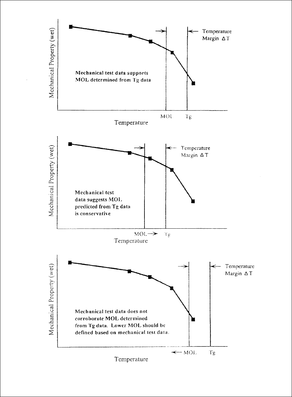
MIL-HDBK-17-1F

Volume 1, Chapter 2 Guidelines for Property Testing of Composites

2-25

FIGURE 2.2.8(c) Use of mechanical and T

data to determine MOL.

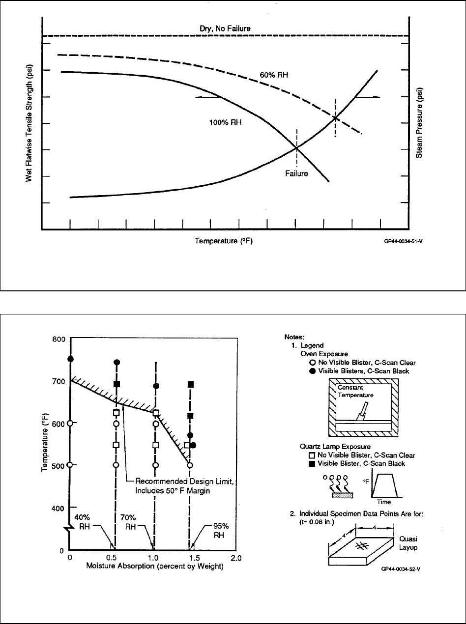
MIL-HDBK-17-1F

Volume 1, Chapter 2 Guidelines for Property Testing of Composites

2-26

FIGURE 2.2.8.1(a) Failure occurs when internal steam pressure exceeds flatwise tensile strength.

FIGURE 2.2.8.1(b) Moisture content limits carbon/polyimide use temperature.

MIL-HDBK-17-1F

Volume 1, Chapter 2 Guidelines for Property Testing of Composites

2-27

The wet

is one of the indicators of a high temperature composite material's MOL. Humidity does

affect the elevated temperature properties and can induce thermal blistering in a thick laminate cross sec-

tion. Thermal blister resistance is a function of the moisture content and thickness of the part, and the

heat up rate the part will encounter.

The other indicators of a high temperature composite material's MOL are the transverse microcrack

(TVM) resistance and thermal oxidative stability (TOS) properties. TVM occurs due to thermal cycling of

the laminate over a temperature range. TVM can develop because of the large difference in coefficient of

expansion between the fiber and resin, and the relative low ductility of most high temperature resins.

These thermal stresses can cause 90° ply failure, which occurs at the fiber-matrix interface. This degra-

dation primarily affects the resin/interface dominated properties like compression strength, in-plane shear

strength, and interlaminar properties. The magnitude of TVM that will occur depends on the application

temperature range, maximum operating temperature, and number of thermal cycles.

TOS is a measure of the oxidation rate of materials, and is also an important property for high tem-

perature composite systems. The thermal oxidation characteristics of a polymeric composite are a func-

tion of fiber, sizing, and resin. The constituents can be evaluated individually for thermal oxidative stability

on a qualitative basis. The actual performance should be evaluated at the laminate level, since the fiber-

matrix interface is the primary area that is degraded. All properties can be affected by TOS, although the

interface dependent properties are most affected. The weight loss of a laminate is a good indication of

the amount of thermal oxidation that has occurred for a particular system, although some mechanical

property degradation may occur prior to significant weight loss. The TOS performance of a material is a

function of the time, temperature, and oxygen flow rate/pressure.

There can be synergistic effects among TVM, TOS, and hot/wet exposures for high temperature

polymeric composites. In order to get an accurate assessment of a material's MOL, it is recommended

these effects be combined in a realistic manner that reflects the actual application environment. For short

term applications, the amount of degradation can be determined experimentally by exposing laminates to

combined conditions of thermal cycling, aging at temperature, and humidity conditioning to the part's spe-

cific mission life. Specimens can be machined and tested from this environmentally exposed material,

and the residual strength of the material can be assessed.

For long term applications, it may be difficult to perform this environmental exposure in real time. Du-

rability modeling and accelerated testing may be required in order to predict end-of-life properties for

these applications. Durability modeling can be used to predict the amount of damage that is generated

as a function of mission exposure conditions, and the subsequent residual strength properties. Mission

exposure testing can be accelerated by aging the material at higher temperature or pressures, in order to

accelerate the oxidation of the material. It is important that the accelerated tests produce realistic dam-

age mechanisms that will be evidenced in real time exposures. For this reason, it is recommended that

some limited real time exposure testing be done in order to confirm the damage mechanisms and also be

used to confirm the durability model's accuracy.

2.2.8.3 Hot Wet Testing - Report Moisture Content at Failure

Laminate specimens to be static strength tested hot, wet are usually preconditioned to an equilibrium

moisture content. Frequently, the test results report the equilibrium moisture content rather than the actual

content at failure. This phenomena is illustrated in Figure 2.2.8.3. The sandwich beam specimens with the

wet carbon/epoxy facesheet in compression were tested at room temperature (RT) and at 350 °F. The five

RT beam compression specimens average moisture content at failure (1.25%) shown in Figure 2.2.8.3 is

same as the moisture content before test since at RT there was no measurable dry out during testing.

This was verified by cutting out a piece of the facesheet immediately after failure, measure the weight,

drying out the piece, and calculating the moisture content at failure. The 350 °F test specimens which

were at the test temperature for 9 minutes until failure, dried out ~ 0.5% from 1.25% to 0.75%. The mois-

ture content for each specimen was determined by cutting out a piece of the facesheet immediately after

failure, measuring the weight, drying out the piece, and calculating the moisture content at failure. One

issue that must be understood is that at the initial moisture equilibrium condition of 1.25 %, every ply

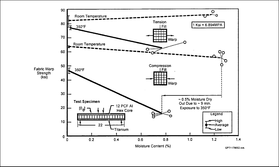
MIL-HDBK-17-1F

Volume 1, Chapter 2 Guidelines for Property Testing of Composites

2-28

through the thickness of the facesheet is at the 1.25 % moisture content. The 0.75 % moisture level at

failure is an average moisture content for a facesheet that has a severe moisture distribution through the

thickness (dry on surface, wet at the center).

FIGURE 2.2.8.3 Moisture dry out during hot/wet strength tests.

The test goal should be to minimize dry out during testing and the potential severe moisture distribu-

tion at failure. There are several ways to minimize the moisture dry out during hot wet testing. If the

strength tests are being conducted at a test temperature below 212 °F, the before test moisture equilib-

rium can be maintained (no dry out) by surrounding the specimen during test with a humidity cabinet at

the same relative humidity used during the original moisture preconditioning. This method will not work if

the test temperature is above 212 °F. Another method to minimize moisture dry out is to minimize the time

at the elevated test temperature. Using contact heaters or quartz lamps (instead of forced hot air cham-

bers) can minimize the time for the specimen surface temperature to reach the test temperature. When

using accelerated heating devices, the mechanical load should not be applied until the center of the test

specimen thickness has been stabilized at the test temperature. Finally, the moisture dry out can also be

minimized by selecting a thicker specimen since the dry out occurs in the surface plies first.

Even though steps have been taken to minimize moisture dry out during hot wet testing, the moisture

content at failure still must be determined and reported with the strength data. There are three ap-

proaches to obtaining the moisture content at failure. One approach is to use moisture monitoring speci-

mens that mimic the material, lay-up, width and thickness of the test section of the test specimen. The

monitoring specimen must follow the identical fabrication and moisture preconditioning steps as the test

specimen. The monitoring specimen should be in the same test chamber as the specimen to follow the

identical thermal history as the specimen during hot wet testing. As soon as the test specimen fails, the

monitoring specimen must immediately be pulled out of the hot environment to preclude additional dry

out. The specimen is weighed, dried out, re-weighed and the moisture content at failure is calculated. A

second approach to obtaining the moisture content at failure is to predict the moisture dry out during hot

wet testing using the documented time temperature history during test and subtract this moisture content

from the moisture content before test to obtain the moisture content at failure. This approach assumes

MIL-HDBK-17-1F

Volume 1, Chapter 2 Guidelines for Property Testing of Composites

2-29

that the moisture diffusion constant for the test temperature is known as well as the detail thermal history

of the specimen during test. The third approach, which is the most accurate and preferred approach, is to

cut a section out of the gage region of the specimen immediately after failure, weigh, dry out, re-weigh

and calculate the moisture content at failure.

2.2.9 Nonambient testing

This section is reserved for future use.

2.2.10 Unidirectional lamina properties from laminates

Though feasible, it is frequently difficult to produce valid or reproducible results on mechanical tests of

unidirectional single-orientation specimens, particularly at testing laboratories lacking the testing volume

to dedicate technicians solely to preparation and conduct of such tests. An alternate approach tests a

crossply laminate, usually from the [90/0]ns-family, and calculates via lamination theory an equivalent

unidirectional lamina strength and stiffness. Crossply laminates have been found to be much more forgiv-

ing of troublesome secondary variations in specimen preparation and testing practice, often yielding

higher mean strengths and lower data scatter. The material response of a crossply laminate is also be-

lieved by many to be more representative of a structural laminate. The basis of test data reduction for this

approach is discussed in Section 2.4.2.

2.2.11 Data normalization

Data normalization is a post-test data manipulation process that attempts to eliminate unrealistic arti-

ficial variation in test data caused by local changes in fiber volume. The details of this process of adjust-

ing fiber dominated results to a fixed reference fiber volume is summarized below and described in detail

in Section 2.4.3.

Most material properties of composites are dependent on the relative proportion of reinforcement and

matrix. In the characterization of properties of a continuously reinforced composite, a portion of the varia-

tion of a property value within a like sample population is simply due to locally changing fiber volume,

rather than due to any variation in fiber, matrix, or fiber/matrix interface properties. For many composite

properties measured in the direction parallel to reinforcing fiber

, the relation between property and fiber

volume is essentially linear. This makes possible a simple adjustment of certain measured properties to a

fixed reference fiber volume, resulting in what is called a normalized property value.

While a minor variation in fiber volume content may be partly due to variation in the absolute amount

of the fiber (and even, to void variation), most fiber volume variation is attributable to locally varying matrix

content as a result of processing.

2.2.12 Data documentation

Planning data documentation requirements and methods prior to the start of a test program is a nec-

essary step for the data to be fully useful for its intended purpose. Before deciding on the scope of data

documentation, the initial purpose for acquiring the data and potential long-term uses of the data must be

determined. Testing requirements may range from obtaining a quick estimate for preliminary material

screening where one or more specimens may suffice to establishing long-term material property values

for an organization's database and submission to MIL-HDBK-17 where large numbers of specimens may

be needed. Different data documentation may be required at different stages of data recording and

evaluation. In the laboratory, raw data, even raw transducer signals, may be stored. For evaluated and

reviewed material properties, less detailed testing information may be needed, particularly if the informa-

tion can be traced back to the original source. Evaluation is used in the sense defined by ASTM Commit-

tee E-49 as “the process of establishing the accuracy and reliability of property data” (Reference

2.2.12(a)). The expectation for MIL-HDBK-17 data is that documentation should be sufficient so that

The so-called "fiber-dominated" properties.

MIL-HDBK-17-1F

Volume 1, Chapter 2 Guidelines for Property Testing of Composites

2-30

1. Traceability and a historical record (identified by manufacture, testing, and evaluation dates) are es-

tablished.

2. The material pedigree and associated process specification are well defined.

3. Testing procedures can be identified.

4. Variables that influence test results are identified.

Other programs that establish reference data should have documentation requirements at least as strin-

gent as those in Table 2.5.6.

In any testing program, for future use of the data to be possible, data documentation should be com-

plete enough so that the material and testing can be reproduced.

Documentation may be recorded in a computerized database for raw data or in a lab notebook or other

hard copy form. The earlier computerization is implemented in the process of storing and evaluating data,

the easier it is to maintain traceability and limit transcription errors. The use of computers does not elimi-

nate the need for error checking and review. Regardless of how much computerization is involved in the

process, each organization should have its own protocol for data recording and review. Considerations

for such a protocol include who is responsible for recording particular information - material identification,

processing, specimen preparation, inspection, testing, and archiving of failed specimens and contact in-

formation for each of these steps. It is quite common for each testing laboratory to have limited access to

material identification information. In this case, responsibility for coordinating material identification infor-

mation with testing laboratory data records must be established if any long-term use of the data is

planned.

Guidance for establishing data documentation requirements is available from several sources. MIL-

HDBK-17, Volume 1, Section 2.5.6 lists data documentation required for data submission to the handbook

as well as a few items that are recommended for in-house recordkeeping. Two ASTM guides (Refer-

ences 2.2.12(b) and (c)) provide primary guidance for data recording and database development. ASTM

E 1309 addresses identification of all composite materials. ASTM E 1434 provides guidance for test in-

formation and results for mechanical properties of continuous-fiber polymer matrix composite materials.

These two documents should be used together in a modular approach. First the material is identified and

then the test method and results information is recorded. Each data element has a level of importance

established by the following categories:

• required for test validity

• required for material traceability

• recommended for test validity

• recommended for material traceability

• optional

These levels of importance divide data documentation requirements into two subsets: one for mate-

rial traceability and one for test validity. A test laboratory can meet requirements for test validity without

access to material identification information. Responsibility for the material traceability should be as-

signed to someone who does have access to the necessary information (as noted above). The approach

used in developing these and similar ASTM guides is to provide assistance for data recording and for the

contents of computerized databases without unduly limiting database structure.

These ASTM guides are implicitly included in the MIL-HDBK-17 data documentation requirements,

since Table 2.5.6 specifies that all sections of the test method are to be followed unless deviations are

reported. Several of the ASTM methods for mechanical properties refer to E 1309 and E 1434 for data

recording. Consequently, the reference flows from Table 2.5.6 to the ASTM test methods to the data-

recording guides.

Another source for guidance is the Composite Material Test Data Schema (CMTDS) developed within

MacNeal Schwendler's MVISION database structure (Reference 2.1.12(d)). Focused on continuous-

fiber polymer matrix composites, this schema establishes specific fields in a defined database structure

MIL-HDBK-17-1F

Volume 1, Chapter 2 Guidelines for Property Testing of Composites

2-31

including field names, synonyms, and values sets for expected field entries without defining levels of re-

quirements. A much larger range of potential properties, including thermal and physical properties, is in-

corporated. The recommendations of MIL-HDBK-17 and the ASTM guides were considered in the devel-

opment of the schema, which functions both as a source of guidance and a specific implementation of

more general recommendations. The released version addresses test data. A draft schema for property

level information is under development. The experience of the CMTDS development is serving as feed-

back into revision of ASTM E 1309 and E 1434 currently underway.

General guidance on the development of material property databases is found in References

2.2.12(e) and (f).

2.2.13 Application specific testing needs

This section is reserved for future use.

2.3 RECOMMENDED TEST MATRICES

2.3.1 Material screening test matrices

The objective of the screening process is to reveal key mechanical property attributes and/or inade-

quacies in new material system candidates, while keeping testing to a minimum. The screening process

identifies, for a particular composite material system, the critical test and environmental conditions as well

as any other special considerations. Proper test matrix design enables comparison with current produc-

tion material systems.

The general approach to screening test matrix design is selection of key static tests that provide suffi-

cient data to assess mean values of stiffness and strength at both the lamina and laminate levels. The

lamina-level tests provide intrinsic material stiffness and strength properties commonly used in classical

lamination plate point stress analysis, including tension, compression, and shear loadings. Both the lam-

ina-level tension tests and open-hole compression tests are also performed at key environments. The

laminate-level tests provide screening strength data on application issues relating to stress discontinuities

such as fastener holes, bolt bearing, or impact damage. Additional laminate level tests provide screening

stiffness data to verify the use of lamina data with classical lamination plate theory for laminate stiffness

predictions. Tests are generally performed at room temperature. Environmental effects are estimated

from the key lamina-level tension and open-hole compression tests.

An example of a typical mechanical property screening test matrix is shown and discussed in Section

2.3.1.1. Under extreme environments, additional factors may have to be considered, as discussed in the

example for high-temperature materials in Section 2.3.1.2. Sensitivity to exposure to operational fluids

and other special issues may justify including additional special tests in the screening evaluation. An ex-

ample of a fluid sensitivity screening test matrix is shown and discussed in Section 2.3.1.3. (Specific ap-

plications may require modifications to the above test matrices.)

2.3.1.1 Mechanical property screening

Table 2.3.1.1 shows a recommended mechanical property screening test matrix developed for epoxy-

based resin systems but also useful for other material systems. In the screening test matrix, 0° axial ten-

sile tests examine fiber dominant properties and 0° axial compression tests monitor fiber/matrix interac-

tions;

both provide static strength and stiffness properties. The ±45° tensile test specimens are used to

evaluate matrix characteristics, determining shear modulus and effective shear strength. Finally, damage

resistance is assessed using compression after impact testing. The testing is conducted under three en-

vironmental conditions: cold temperature ambient (CTA), room temperature ambient (RTA), and elevated

temperature wet (ETW). These test conditions are recommended based on results for current epoxy

The 0° axial tensile tests may reveal fiber/matrix interaction in some materials at high strain rates.

MIL-HDBK-17-1F

Volume 1, Chapter 2 Guidelines for Property Testing of Composites

2-32

resin systems that show the CTA environment as critical for fiber dominated properties and the ETW envi-

ronment as the most severe condition for matrix dominated properties. The ETW specimens are condi-

tioned to moisture equilibrium at the specified relative humidity.

TABLE 2.3.1.1 Composite material static strength screening test matrix.

Test Number of Specimens Evaluation Emphasis

CTD RTA ETW

Lamina:

0° Tension 3 3 3 fiber

0° Compression 3 fiber/matrix

±45° Tension 3 fiber/matrix

(0°/90° shear - lamina)

(±45° - laminate)

Laminate:

Open Hole

Compression

3 3 stress riser

Open Hole

Tension

3 stress riser

Bolt-Bearing

3 bearing

Compression after

Impact

3 impact damage

Fastener hole effects

per NASA Reference Publication 1092.

2.3.1.2 Mechanical property screening for high-temperature material systems

Table 2.3.1.2 shows a typical mechanical property test matrix intended for high temperature polymer

matrix composites. The changes were made to Table 2.3.1.1 in order to properly assess the durability of

high temperature polymer matrix composites during the screening stages of an evaluation. The test ma-

trix may vary depending on the purpose of the investigation, but it is important that all exposure conditions

be evaluated.

Prior to the mechanical test evaluation, it is necessary to evaluate prepreg physical and laminate

properties. Test laminates should be carefully inspected for porosity content, dry

, and wet T

. The rec-

ommended mechanical tests cover fiber-dominated, interface/resin-dominated, and damage tolerance

properties. The elevated test temperature static test conditions should be set below the wet

of the sys-

tem.

The wet exposure condition is 160°F (71°)/ 85% relative humidity to an equilibrium weight gain. It is

very important that specimen dry-out be measured and kept to a minimum during the elevated tempera-

ture wet tests.

MIL-HDBK-17-1F

Volume 1, Chapter 2 Guidelines for Property Testing of Composites

2-33

TABLE 2.3.1.2 Composite material test matrix for high temperature PMC's.

Mechanical Property Dry Test Temperature Wet

TOS

Thermal Cycle

Minimum

Temp

75°F

(24°C)

ET1 ET1 ET1 ET1

Tension 3 3 3 - 3 -

Compression or OHC - 3 3 3 3 3

In-Plane Shear - 3 3 3 - 3

Mode I Fracture

Toughness or CAI

- 3 3 - 3 3

1 - ET1 Elevated test temperature should be less than the Wet Glass Transition Temperature of the

material

2 - Laminates are to be thermally aged at a temperature greater than ET1 but less than the dry

for

a minimum of 1000 hours or an accelerated test condition that represents a 1000 hour exposure.

Weight loss should be recorded as a function of time, i.e., 100, 250, 500, 750 and 1000 hours.

Microscopy should be performed after exposure. Specimens are to be machined after exposure.

3 - Laminates are to be thermal cycled from Min Temp to a temperature greater than ET1 but less

than the dry

. Laminates are to be cycled for a minimum of 500 thermal cycles. Microcrack

density is to be measured after cycling. Specimens are to be machined from the laminate after

exposure.

The thermal oxidative stability (TOS) test should be performed for a minimum of 1000 hours. Weight

loss should be measured during testing at specified intervals of 100, 250, 500, 750, and 1000 hours. This

test provides a measurement of the oxidation rate of the material.

Thermal cycling should be done for a minimum of 500 thermal cycles. The purpose of the test is to

determine the rate of microcracking, not only if microcracking will occur. The minimum temperature

should represent the minimum temperature of the potential application, for example, -65°F (-54°C) for

aircraft.

The maximum exposure temperature for both the TOS and thermal cycling test should be between

the wet

and dry T

of the material system. If the exposure temperature is below the wet T

, the test

may not be discriminating enough and longer exposure times may be necessary. Exposures above the

dry

of a material normally provide an unrealistic damage mechanism that does not occur below the dry

of the material. Prior to the machining of specimens, laminates should be non-destructively inspected

for porosity and delaminations. Microscopy should also be done in order to understand the damage

mechanism associated with the specific exposure. This will include the measurement of microcrack den-

sity.

2.3.1.3 Fluid sensitivity screening

Historically, the concern over exposure of structural composite materials to commonly encountered

service related fluids other than water or moisture has not been a major concern. This is because the

majority of structural composites have had an epoxy resin matrix which has inherently been very fluid re-

sistant. With the epoxies, in general, the allowance for property degradation caused by absorption of at-

mospheric moisture has been sufficient to cover degradation which might be caused by other pertinent

fluids, e.g., fuel, hydraulic oil, etc. Although epoxy resin systems are subject to accelerated degradation

in the presence of highly acidic media, the majority of service fluids tend to be basic in nature, e.g., clean-

MIL-HDBK-17-1F

Volume 1, Chapter 2 Guidelines for Property Testing of Composites

2-34

ing solvents and hydraulic fluids. The poor resistance of epoxies to methylene chloride, a common ingre-

dient in paint strippers, is an exception. Methylene chloride also aggressively attacks other structural

polymers. Consequently, the use of chemical paint strippers on polymer matrix composites is generally

not allowed.

With due consideration of the above, it is still important to evaluate the resistance of new polymer ma-

terials to fluids with which they might come in contact. Many new epoxies have components, added to

improve properties such as toughness, which might affect their solvent resistance. Many other polymers,

which have different solvent sensitivities, are also now being used or are being considered for use. An

example of a problem encountered in the past was that associated with the developmental evaluation of

polysulfone thermoplastic structural parts and their abandonment due to poor resistance to phosphate

ester based hydraulic fluids (Reference 2.3.1.3(a)). Some other structural thermoplastics, although they

have excellent resistance to moisture and hydraulic oils, have poorer resistance to fuels. Fuels with

higher aromatic content, e.g., JP-4 as compared to JP-8, seem to cause the worst problems (Reference

2.3.1.3(b)). In the referenced case, the fuel exposure seemed mostly to effectively lower the material's

(PEEK) glass transition temperature (Reference 2.3.1.3(c)). The result was comparable lowering of the

material's maximum use temperature.

Higher service temperature resin systems such as bismaleimides (BMI's) and polyimides are suscep-

tible to degradation by fluids with high alkalinity. Both polymer formulations are susceptible to a cleavage

of the functional imide rings in the presence of high concentrations of hydroxide ions. This is significant

for two reasons. First, cleaning solvents and hydraulic fluids used by most airlines are alkaline by nature

and second, hydroxide ions are produced locally at the resin boundary during galvanic coupling between

carbon fibers and active metals and can cause degradation. The galvanic corrosion situation should be

satisfactorily manageable with an attentive design. The incorporation of an isolation mechanism such as

a resin/fiber ply between the carbon/resin and metal structure is one approach to mitigating the risk asso-

ciated with the electrolytic driven degradation. Exposure can be lessened by providing drainage, etc. It is

important that the laminate edges be well sealed if there is exposure in a sump area. In general, the ex-

posure of these materials to alkaline solutions may be sufficiently incidental that this also may not be a

problem.

The following evaluation procedure is suggested to assess the suitability of polymer resin systems for

application where they might be exposed to a harmful fluid environment.

The evaluation should account for different exposure levels of aircraft structure to fluids. Two fluid

exposure classifications are suggested, with example fluids cited for each group:

Group I

Fluids that have the potential for pooling or will contact the material for an extended period of time.

JP-4 Jet Fuel MIL-T-5624

JP-5 Jet Fuel MIL-T-5624

JP-8 Jet Fuel MIL-T-83133

Hydraulic Fluid MIL-H-5606

Hydraulic Fluid

MIL-H-83282

PAO (Poly Alphaolefin) Cooling Fluid MIL-C-87252

Engine Lubricating Oil MIL-L-7808

Engine Lubricating Oil MIL-L-23699

Ethylene Glycol/Urea Deicer (Class I) SAE AMS 1432 (superseding MIL-D-83411)

Sump Water

MIL-S-8802 section 4.8.15

Methylene Chloride

ASTM D4701 (superseding MIL-D-6998)

SO2/Salt Spray

---

Monsanto low-density aviation hydraulic fluid, commercial.

A mixture of SAE AMS 2629 Jet Reference Fluid and 3% sodium chloride/water solution.

U.S. Navy requirement.

MIL-HDBK-17-1F

Volume 1, Chapter 2 Guidelines for Property Testing of Composites

2-35

Group II

Fluids that are wiped on and off (or evaporate) or will not contact the material for an extended period

of time.

Alkaline Cleaner (Types 1 and 2) MIL-C-87936

MEK Washing Liquid ASTM D740 (superseding TT-M-261)

Dry Cleaning Solvent (Type 2) P-D-680

Hydrocarbon Washing Liquid TT-S-735

Polypropylene Glycol Deicer (Type 1) MIL-A-8243

Isopropyl Alcohol Deicing Agent TT-I-735

More information on these fluids is found in References 2.3.1.3(d) - (t).

Exposure by immersion prior to test or to evaluate weight loss is also recommended, using a different

exposure level for each group:

Group I Immerse material in fluid until it reaches equilibrium weight gain (saturation). (Except for

the MIL-S-8802 Sump Water corrosion test.)

Group II Immerse material in fluid for 15 days to determine worst case effects. Then follow-up with

tests that simulate a more realistic exposure including accidental extended exposure.

Both mechanical and physical testing should be done. Mechanical testing should include open hole

compression tests on quasi-isotropic lay-up specimens and ±45° tension specimens. The open hole

compression test has a meaningful relation to design values and is sensitive to matrix degradation. The

use of a ±45° tension test is commonplace in industry for comparison of matrix properties. It is a sensitive

test which will identify "potentially" harsh fluids. It provides an indication of whether necessary shear stiff-

ness has been retained to ensure acceptable resin to fiber property transfer. While a material stiffness

loss criterion is material and application specific, a 20-40% loss in shear modulus from that of the unex-

posed material is generally considered significant, and should be further investigated. A minimum of five

specimens should be tested after exposure at room temperature and at the maximum use temperature.

The results should be compared with unexposed controls.

A more economical alternative to open hole compression and ±45° tension testing is interlaminar or

short beam shear tests. These specimens are easily fabricated, machined, conditioned, and tested. Al-

though not as generally related to design properties, short beam strength tests are sensitive to matrix

degradation and can be valuable indicators for material evaluation. As with the ±45° tension tests, results

after exposure should be compared to unexposed controls at room and elevated temperature to obtain

fluid exposure effects.

Physical testing should include weighing to measure weight change, photomicrographs to examine

for microcracks, and, where practical, scanning electron microscopy to examine for surface crazing.

Relative to the former, it must be warned that because a saturation condition has apparently been

reached, it does not automatically follow that further degradation of properties has ceased. Especially

where new resin systems are involved, test with long term exposure to critical fluids should be conducted.

An example of such testing is given in Reference 2.3.1.3(u). Due to the long exposure times involved,

these tests should be started early in the evaluation process.

It has been the procedure in the past that if water or moisture has been proven to be the most prop-

erty-degrading fluid, then fluid exposure tests involving other than moisture conditioning were not included

in subsequent design testing. Such a procedure for Group I pooling fluids is presented in Figure

2.3.1.3(a). In effect, if the properties of the material after fluid exposure are better than after moisture ex-

posure, then subsequent testing accounts for moisture only. If a fluid other than water is more critical,

then subsequent testing must include evaluation with that fluid.

MIL-HDBK-17-1F

Volume 1, Chapter 2 Guidelines for Property Testing of Composites

2-36

In the case of Group II wipe on/wipe off fluids, the procedure is somewhat different since water is not

a good comparison. Consequently, comparison to a resin that has an acceptable service history is rec-

ommended. This is illustrated by the decision tree in Figure 2.3.1.3(b) where comparison with the per-

formance of 3501-6 epoxy resin system is suggested.

FIGURE 2.3.1.3(a) Decision tree to closure - Group I pooling fluids.

MIL-HDBK-17-1F

Volume 1, Chapter 2 Guidelines for Property Testing of Composites

2-37

FIGURE 2.3.1.3(b) Decision tree to closure - Group II fluids without long term exposure.

MIL-HDBK-17-1F

Volume 1, Chapter 2 Guidelines for Property Testing of Composites

2-38

2.3.2 Material qualification test matrices

2.3.2.1 Constituent test matrix

This section is reserved for future use.

2.3.2.2 Prepreg test matrix

The recommended test matrix for prepreg materials is shown in Table 2.3.2.2. The table is based on

thermosetting matrices and requires modification for thermoplastic matrices.

TABLE 2.3.2.2 Recommended physical and chemical property tests to be performed

by material supplier and prime contractor.

Test

Property

Suggested

Test

Procedure

Number of

Tests per

Batch

Total Number of

Tests

Resin Content ASTM D 3529 3 15

Volatile Content ASTM D 3530 3 15

Gel Time ASTM D 3532 3 15

Resin Flow ASTM D 3531 3 15

Fiber Areal Wt.

3 15

Moisture Content

3 15

Tack

3 15

HPLC (High Performance Liquid

Chromatography)

3 15

IR (Infrared Spectroscopy)

3 15

DMA (Dynamic Mechanical

Analysis, neat resin only)

3 15

DSC (Differential Scanning

Calorimetry)

3 15

RDS (Rheological Dynamic

Spectroscopy)

3 15

Test procedures should be coordinated and agreed to prior to manufacture of prepreg material.

Tests should be performed on each of the five batches of prepreg material.

gTest procedures to be described at a later date.

MIL-HDBK-17-1F

Volume 1, Chapter 2 Guidelines for Property Testing of Composites

2-39

2.3.2.3 Lamina test matrices

Recommended physical and mechanical property test matrices for statistical evaluation of lamina-

level materials are shown in Tables 2.3.2.3(a) and 2.3.2.3(b).

The mechanical test matrix shown in Table 2.3.2.3(b) is based on a minimum of thirty tests per condi-

tion per property (at least six replicates for each of at least five batches) to provide for paramet-

ric/nonparametric analysis when determining B-basis properties. Fewer replicates or batches may be

acceptable if agreed to between the contractor and the procuring or certifying agency.

TABLE 2.3.2.3(a) Cured lamina physical property tests.

Physical Property Suggested Test

Procedure

Number of Tests

Per Prepreg Batch

Total Number

of Tests

Fiber Volume ASTM D 3171 3 15

Resin Volume ASTM D 3171 3 15

Density ASTM D 792 3 15

Cured ply thickness - 10 50

Glass Transition

Temperature (dry)

- 3 15

Glass Transition

Temperature (wet)

- 3 15

1. Tests should be performed on each of the five batches.

2. Dry specimens are "as fabricated" specimens which have been maintained at ambient conditions

in an environmentally-controlled test laboratory. Wet specimens are environmentally conditioned

by exposing them in an elevated temperature humidity chamber until they attain an equilibrium

moisture content agreed to by the contractor and customer, then packaged in a heat-sealed alu-

minized polyethylene bag until required for test. Tests should be performed in a manner which

maintains the moisture content in specimens at the levels agreed to by the contractor and certify-

ing agency.

MIL-HDBK-17-1F

Volume 1, Chapter 2 Guidelines for Property Testing of Composites

2-40

TABLE 2.3.2.3(b) Cured lamina mechanical property tests.

Mechanical

Property

Test

Methods

Test Condition

and

Number of Tests

Per Batch

Number

of Tests

See

Handbook

Section

Min. Temp

Dry

Max. Temp

Wet

0° Tension (warp) 6.7.4.4

6 6 6 90

90° Tension (fill) 6.7.4.4

6 6 6 90

0° Compression (warp) 6.7.5.4 6 6 6 90

90° Compression (fill) 6.7.5.4 6 6 6 90

In-plane Shear 6.7.6.4 6 6 6 90

0° Short Beam Shear 6.7.6.4 - 6 - 30

480

1. MIL-HDBK-17 is not currently in a position to make exclusive test method recommendations,

but the referenced Handbook sections identify methods that are currently deemed acceptable

for data submittals to MIL-HDBK-17.

2. Minimum and maximum temperature tests should be performed within ±5°F (±2.8°C) of the

nominal test temperature. Nominal test temperatures will be as agreed to by contractor and

certifying agency. Dry specimens are "as-fabricated" specimens which have been maintained

at ambient conditions in an environmentally-controlled test laboratory. Wet specimens are en-

vironmentally-conditioned by exposing them in a humidity chamber until they attain an equilib-

rium moisture content agreed to by the contractor and certifying agency, and then packaging

them in a heat-sealed aluminized polyethylene bag until required for test. Tests should be

performed in a manner which maintains the moisture content in specimens at the levels

agreed to by the contractor and certifying agency.

3. Tests should be performed on each of the five batches.

4. For 0° and 90° tension, ASTM D

3039 and SACMA Recommended Method (SRM) 4-88 are

acceptable test methods for MIL-HDBK-17 data submittals.

5. Short Beam Shear is for screening and quality control purposes only.

MIL-HDBK-17-1F

Volume 1, Chapter 2 Guidelines for Property Testing of Composites

2-41

2.3.2.4 Filament-wound materials test matrix

The test matrix shown in Table 2.3.2.4 contains the suggested mechanical property tests for filament

wound structures.

TABLE 2.3.2.4 Filament-wound materials property tests.

Mechanical

Property

Suggested Test

Procedure

Test Condition and

Number of Tests Per Batch

Number

of Tests

Condition

Min. Temp

Dry

Max. Temp

Wet

0° Tension ASTM D

3039 6 6 6 90

90° Tension ASTM D

5450 6 6 6 90

0° Compression ASTM D

3410

(Method B)

6 6 6 90

90° Compression ASTM D

5449 6 6 6 90

In-plane Shear ASTM D

5448 6 6 6 90

Interlaminar Shear ASTM D

5379 6 6 6 90540

1 Reader is referred to Section 6.7 Mechanical Property Tests for more information on these

ASTM test methods

2 Tests should be performed on each of the five batches.

3 Minimum and maximum temperature tests should be performed within ±5°F (±2.8°C) of the

nominal test temperature. Nominal test temperatures will be as agreed to by contractor

and certifying agency. Dry specimens are "as-fabricated" specimens which have been

maintained at ambient conditions in an environmentally-controlled test laboratory. Wet

specimens are environmentally-conditioned by exposing them in a humidity chamber until

they attain an equilibrium moisture content agreed to by the contractor and certifying

agency, and then packaging them in a heat-sealed aluminized polyethylene bag until re-

quired for test. Tests should be performed in a manner which maintains the moisture con-

tent in specimens at the levels agreed to by the contractor and certifying agency.

The JANNAF Composite Motorcase Subcommittee has recommended to filament wind the flat lami-

nates used for the test articles for ASTM D 3039, ASTM D 3410 and ASTM D 5379 for the uniaxial mate-

rial properties used in the design and analysis of filament wound structures. However, there are no uni-

versal standards describing the process. Consequently there are numerous methods used by industry

and Government to manufacture the flat laminates, (References 2.3.2.4(a) and (b)). At these two meet-

ings filament winders, both industry and government, presented their techniques to prepare flat laminates

for the purpose of testing for uniaxial mechanical material properties.

One main issue is whether to use a cylindrical or a rectangular winding mandrel. If a cylindrical man-

drel is used, the diameter of the mandrel is a factor. The larger the diameter, the less the effects of shear

when the laminates are removed from the winding mandrel and flattened for curing. If the mandrel is rec-

tangular, the main concern is how tension of the fiber is maintained during winding.

MIL-HDBK-17-1F

Volume 1, Chapter 2 Guidelines for Property Testing of Composites

2-42

The following issues have been identified as concerns for filament wound laminates:

• autoclave vs. non-autoclave cure

• cutting of fibers before or after cure

• whether to cure on the winding mandrel or to remove and cure on a separate fixture

• whether to use a caul plate

• whether to wind single layers, cut and stack versus winding entire thickness before cutting

Currently the winders appear to be using the technique that produces a panel that most closely simu-

lates the process used on their finished part. The ASTM Task Group D30.04.05 is discussing and pursu-

ing these same issues and developing a standard method to prepare filament wound laminates.

2.3.3 Material acceptance test matrices

This section is reserved for future use.

2.3.4 Alternate material equivalence test matrices

2.3.4.1 Qualification of alternate source composite materials

2.3.4.1.1 Introduction

These guidelines apply to the situation where one composite material system from a single supplier

has been qualified and it is necessary or desirable to qualify an alternate system and/or supplier. The

approach assumes the existence of a body of data and experience developed with the original material

(none exists for the alternate system) from which the mechanical property basis values have been devel-

oped. It also assumes higher level tests have been performed to qualify a product and verify its perform-

ance.

A drastic change, such as switching fiber from E-glass to aramid, is not covered by this guideline.

The focus is on materials that will meet the original material specification. A fiber class change, or compa-

rable substitution, is considered a major revision or redesign. Processing and tooling changes are also

considered beyond the scope of this section.

2.3.4.1.2 Goal and approach

The ultimate goal in qualifying an alternate material is to be able to exchange this material with the

original system without compromising manufacturing or structural performance. To accomplish this goal it

is necessary to define the key material parameters that govern performance during specific phases, such

as processing, manufacturing, and service. The ideal is to perform this evaluation at the material con-

stituent or composite lamina levels by measurement and comparison of parameters like chemical compo-

sition, fiber strength, matrix strength, and composite strength. This may be possible in the future, but is

not adequate with current technology.

Successful qualification of an alternate material will not, in itself, be sufficient to permit mixing of this

system with the original material within a given part. Intermixing of two different material systems within

the same part is not recommended unless appropriate evaluations are carried out to demonstrate com-

patibility.

The focus of MIL-HDBK-17 is B-basis lamina properties. Adequate alternate material qualification

may require going beyond this level of evaluation into more complex demonstrations involving analysis

and tests. These may include laminate, specimen, element, and subcomponent tests such as open hole,

filled hole, bolt bearing, low velocity impact, fatigue, and panel buckling. The general approach to be fol-

lowed for qualification of an alternate material is as follows:

1. Identify the key material performance parameters and why they are crucial.

MIL-HDBK-17-1F

Volume 1, Chapter 2 Guidelines for Property Testing of Composites

2-43

2. Define appropriate tests, measurements, or evaluations for each of the parameters. These must

correspond exactly to the tests, measurements, or evaluations performed on the original material

(for example: same specimen type and same conditions).

3. Define pass/fail (success) criteria for the tests, measurements, and evaluations.

4. Prepare a test plan and obtain necessary approvals.

5. Perform tests and document results.

6. Accept or reject.

2.3.4.1.3 Material compatibility

The extent to which an alternate material used in hardware applications must be evaluated to demon-

strate equivalence, or superiority, with the original system is first, a function of its material compatibility

and second, a function of hardware structural complexity and loading. Material compatibility is defined by

the criteria shown in Table 2.3.4.1.3. The baseline system is a material from a single prepregger using a

specific prepreg production line. For example, AS4/3501-6 produced from line 3 at Hercules, Inc. The

most compatible alternate material, and the one requiring the minimum to demonstrate equivalence would

be AS4/3501-6 produced from line 4 at Hercules, Inc. The least compatible material system would be one

from a different prepregger with a different matrix and fiber. Thus, Fiberite C12K/934 is a less compatible

system and requires more effort to demonstrate equivalence. Situations not included in Table 2.3.4.1.3

must be evaluated with respect to their appropriate compatibility scale.

2.3.4.1.4 Key material or structural performance parameters

Key material or structural performance parameters are those measurable quantities which, if com-

pared to the original values, can be used to quantify any difference in manufacturing or structural per-

formance parameters, are material and hardware dependent, and may change with design, tooling,

manufacturing, and usage factors. However, five categories of parameters have been defined in Table

2.3.4.1.4. This table lists examples of typical performance parameters appropriate for each category.

2.3.4.1.5 Success criteria

The relative importance and completeness of performance parameters varies with the part design,

loading, and application. In some cases it is sufficient merely to report a measured value. In other cases

the value must meet or exceed the original measurement. And in some cases the value must not vary

significantly either higher or lower than the original value. As an example, this is generally true for

modulus, fiber areal weight, matrix content, and cured ply thickness.

Success criteria for each parameter must be defined at the beginning of the qualification program.

Justification for each success criteria imposed must be provided. A tolerance on a given measurement

should be part of the success criteria.

MIL-HDBK-17-1F

Volume 1, Chapter 2 Guidelines for Property Testing of Composites

2-44

TABLE 2.3.4.1.3 Material compatibility criteria.

MOST COMPATIBLE LEAST COMPATIBLE

MATERIAL FACTOR 1 2 3 4 5 6

Fiber Type Y N Y N Y N

Fiber Tow Size Y Y/N Y Y/N Y N

Resin Y Y N Y N N

Prepregger N Y Y N N N

Production Line N Y Y N N N

Y - remains the same in alternate material

N - changes in alternate material

a) Column 1 is a change in prepreg supplier and production line. This situation is becoming more com-

mon today as resin systems are licensed between prepreg manufacturers; for example, the Navy's

A-6 re-wing and V-22 Osprey programs where Hercules 3501-6 is licensed to ICI Fiberite. This coop-

erative licensing allows competitive bidding for prepreg supplies and provides the customer with

nearly identical prepreg for production usage.

b) Column 2 represents a change in fiber type based on a new fiber with properties similar to the origi-

nally qualified fiber. This situation may occur for economic reasons or in the event of discontinued fi-

ber supply.

c) Column 3 is a change in resin. This would be justified by development of new resin systems by the

prepregger that would offer improved pricing and/or properties, such as damage tolerance, for the

customer's program.

d) Columns 4 and 5 represents a change in prepreg supplier, production line, and fiber or resin. This

situation would occur when a customer needs and additional supplier but wishes to use the same fi-

ber or resin due to second-source qualification budget constraints (assumes existing data base on the

resin and/or fiber). Again, economic reasons justify this situation.

e) Column 6 involves qualifying a new source prepregger using a different fiber and resin system. An

example of this situation is qualifying Fiberite C12K/934 to replace Hercules AS4/3501-6. This is the

least compatible situation and would require the greatest effort to demonstrate acceptability.

MIL-HDBK-17-1F

Volume 1, Chapter 2 Guidelines for Property Testing of Composites

2-45

TABLE 2.3.4.1.4 Examples of key material or structural performance parameters.

PHYSICAL PROCESSING MECHANICAL MANUFACTURING HARDWARE

SCALE-UP

TACK CURED PLY

THICKNESS

LAMINA PROPERTIES DRILLING STATIC

STRENGTH

RESIN CONTENT CURE CYCLE ENVIRONMENTAL

EFFECTS

TOOLING FATIGUE

STRENGTH

AREAL WEIGHT SENSITIVITY DAMAGE TOLERANCE NONDESTRUCTIVE

INSPECTION

STIFFNESS

FLOW FIBER VOLUME INTERLAMINAR SHEAR COST FAILURE MODES

GLASS TRANSITION

TEMPERATURE

THERMAL

CYCLING

FLATWISE TENSION LEAD TIME QUALITY

FORM DENSITY FLAW GROWTH AVAILABILITY BEARING

OUT TIME EXOTHERM EFFECT OF DEFECTS REPEATABILITY CRIPPLING

SHELF LIFE TOXICITY PRESSURE BOTTLE

TESTS

MACHINABILITY OPEN HOLE

TENSION

STORAGE

REQUIREMENTS

UNIFORMITY OPEN HOLE

COMPRESSION

MOISTURE

ABSORPTION

PANEL TESTS

SOLVENT

RESISTANCE

FATIGUE TESTS

2.3.4.1.6 Lamina-level test matrices for alternate material assessment

Section 2.5 defines minimum requirements for B-basis lamina property values for MIL-HDBK-17 data,

which can be quickly summarized as thirty specimens from at least five batches of material for each envi-

ronment and property of interest. Since an alternate material qualification program is not intended to es-

tablish basis values, but rather to show compliance with them, a reduced number of lamina tests can be

allowed for a second population of data to be compared to the original data. The actual number of

equivalency tests needed depends on the degree of compatibility between the two material systems.

Recommendations for test quantities and properties for tape and fabric material forms are shown in Ta-

bles 2.3.4.1.6(a) and (b). The equivalency check tests must be performed in the same way, and using the

same test methods, as the tests used to determine the basis values. Following testing, (see Section

8.4.3) appropriate statistical analysis must be performed to evaluate the test results and assess equiva-

lency.

MIL-HDBK-17-1F

Volume 1, Chapter 2 Guidelines for Property Testing of Composites

2-46

TABLE 2.3.4.1.6(a) Alternate material lamina test requirements - tape.

No. of Batches

Replicates

Environments

Total

Lamina Property

Compatibility

1 2 3 4 5 6

Compatibility

1 2 3 4 5 6

Compatibility

1 2 3 4 5 6

Compatibility

1 2 3 4 5 6

0° Tension

90° Tension

0° Compression

90° Compression

In-Plane Shear

2 3 3 3 3 3

4 4 4 5 5 6

2 2 2 2 2 2

16 24 24 30 30 36

80 120 120 150 150 180

Compatibility is defined in Table 2.3.4.1.3.

The environments should be RTD and the worst case.

Quality assurance tests must be performed per individual specification.

MIL-HDBK-17-1F

Volume 1, Chapter 2 Guidelines for Property Testing of Composites

2-47

TABLE 2.3.4.1.6(b) Alternate material lamina test requirements - fabric.

No. of Batches

Replicates

Environments

Total

Lamina Property

Compatibility

1 2 3 4 5 6

Compatibility

1 2 3 4 5 6

Compatibility

1 2 3 4 5 6

Compatibility

1 2 3 4 5 6

Warp Tension

Fill Tension

Warp Compression

Fill Compression

In-Plane Shear

2 3 3 3 3 3

- 3 3 3 3 3

2 3 3 3 3 3

- 3 3 3 3 3

2 3 3 3 3 3

4 4 4 5 5 6

- 4 4 5 5 6

4 4 4 5 5 6

- 4 4 5 5 6

4 4 4 5 5 6

2 2 2 2 2 2

- 2 2 2 2 2

2 2 2 2 2 2

- 2 2 2 2 2

2 2 2 2 2 2

16 24 24 30 30 36

- 24 24 30 30 36

16 24 24 30 30 36

- 24 24 30 30 36

16 24 24 30 30 36

48 120 120 150 150 180

Compatibility is defined in Table 2.3.4.1.3.

The environments should be RTD and the worst case.

Quality assurance tests must be performed per individual specification.

MIL-HDBK-17-1F

Volume 1, Chapter 2 Guidelines for Property Testing of Composites

2-48

2.3.4.1.7 Laminate-level test matrices for alternate material assessment

The next higher level of testing that should be considered for qualification of an alternate material sys-

tem is laminate mechanical properties. This level of testing confirms strength (strain) basis values for

strategic design parameters and should be performed using the same laminate tested for the original ma-

terial. The recommended tests are shown in Table 2.3.4.1.7(a). The extent to which the Table

2.3.4.1.7(a) tests are performed is governed by the material compatibility factor. The recommended num-

ber of tests is given in Table 2.3.4.1.7(b).

TABLE 2.3.4.1.7(a) Extent of laminate testing.

Material

Compatibility

Laminate Tests

Total

Factor Tape Fabric

1 Unnotched Laminates 12 12

2, 3 All Static Test, Two Environments 36 36

4, 5 All Static Test, Two Environments 36 36

6 All Required 42 42

2.3.4.1.8 Alternate material evaluation summary

Many of the handbook recommendations on key material performance parameters, such as physical

and processing characteristics, are commonly included in material and process specifications. Other pa-

rameters are more application related and may be difficult to demonstrate at the material level. The

reader should not infer from lack of discussion that a particular topic is unimportant; all key performance

parameters for a specific project or product must be considered.

Guidelines for substantiating lamina and laminate material property requirements, given some change

in the material system or process, were provided. Higher level mechanical element/subcomponent sub-

stantiation tests may also be required, depending on the degree of change in the key material or struc-

tural parameter, and on the application.

Statistical methods for comparing batches are discussed in Section 8.4.3.

2.3.4.2 Evaluation of changes made to previously qualified materials

This section defines guidelines for evaluating changes made by a material supplier to a material sys-

tem provided as a qualified source. A drastic change is not covered herein. The focus is to meet original

(existing) material specification requirements. Potential changes at all levels should be considered.

The goal of the recommended evaluations is to verify that intended changes do not compromise

physical, structural, or manufacturing requirements. This guideline provides a list of potential changes

and appropriate experiments/tests to evaluate the effects of a particular change. Specific evaluations are

tailored to the nature and severity of proposed changes.

MIL-HDBK-17-1F

Volume 1, Chapter 2 Guidelines for Property Testing of Composites

2-49

TABLE 2.3.4.1.7(b) Number of suggested laminate tests.

Design Property Loading No. of Laminate Types No. of

Environments

Replicates

Total Number of

Specimens

Tension Compression Tape Fabric Tape Fabric

Static

Unnotched laminate,

strength and stiffness

X X 1 1 2 3 12 12

Open Hole X 1 1 2 3 6 6

Filled Hole X 1 1 2 3 6 6

Impact Damage X X 1 1 1 3 6 6

Double Shear Bearing X 1 1 1 3 3 3

Single Shear Bearing X 1 1 1 3 3 3

36 36

Fatigue

Open Hole - - 1 1 1 3 3 3

Impact Damage - - 1 1 1 3 3 3

6 6

42 42

Where two environments are required, they should be RTD and worst case. Where one is required, it should be RTD.

One batch of material is sufficient.

Repeated load and residual strength: constant amplitude, R = -1, n = 1 x 10

cycles.

MIL-HDBK-17-1F

Volume 1, Chapter 2 Guidelines for Property Testing of Composites

2-50

A documented quality plan is an assumed prerequisite for this procedure. It should describe the

manufacturing process from raw materials receiving to final product shipment. This document should be

kept current. It should be in accordance with ISO 9002 or Mil-Q-9858A. The quality plan should refer-

ence raw materials used, show key manufacturing steps in proper sequence, and list critical process con-

trol documentation as well as quality inspection or testing.

At the time of a proposed modification, a process analysis should be done to determine if the pro-

posed change warrants further consideration. This can be done by an appropriate technical specialist.

Guidelines for screening possible modifications should be established prior to embarking on an evaluation

program. For example, routine or ongoing maintenance of equipment, changes in personnel, or upgrad-

ing control instrumentation would not normally require formal evaluation. Proposed changes in product

formulation, elimination of process steps, changes in manufacturing equipment, or changes in sequence

of operations are the types of significant modifications that would require formal evaluation.

The relative importance or category of a proposed process modification is determined by a logical

system of in-depth process and product impact analysis. It is recommended that a process review team

(PRT) be established to perform the process analysis. The process analysis must identify:

• Key process steps (including sequence)

• Key equipment used at each process step.

• Quality-critical processing parameters for each piece of equipment (time, temperature, rate, pres-

sure).

• Quality-critical operating ranges for each critical process parameter.

• Quality-critical instrumentation used for monitoring and/or controlling each critical process pa-

rameter.

2.3.4.2.1 Modification categories

When a proposed process modification is identified for consideration, a comprehensive review of all

related information should be conducted. This includes the rationale for making the process modification.

An appraisal should be made as to the impact that the change could have on the next product user as

well as upon the product's performance in the final application.

The foundation of the review is derived from the knowledge obtained from the product/process analy-

sis described previously. Based upon this product impact review, the process modification will be placed

into one of the following three categories:

Category 1: "No Impact"

The modification is minor in nature. It is known not to impact the product's quality, physical or chemi-

cal properties or performance. Additionally, the modification is not likely to cause operational or product

performance deficiencies for subsequent customers. This type of process modification is therefore classi-

fied as "No Impact".

Category 2: "Unknown"

If upon review of available information there is not enough known about the proposed change, then

the modification must be classified as "Unknown".

Category 2 is a temporary classification which is held until additional information is made available.

No modification classified as Category 2 should be implemented. All Category 2 classifications must

eventually become Category 1 or 3 before the modification is implemented.

MIL-HDBK-17-1F

Volume 1, Chapter 2 Guidelines for Property Testing of Composites

2-51

Category 3: "Change"

If upon review of available information it is decided that the proposed modification may result in a sig-

nificant change to the product's properties, quality, performance, or may have an impact on subsequent

customers, then the modification must be classified as a "change".

2.3.4.2.2 Actions required for each modification category

Category 1 modifications should be formally approved. The change should be documented and an

appropriate process change follow-up or monitoring file initiated. This releases manufacturing to imple-

ment the modification at an agreed upon schedule with appropriate monitoring for a specified time.

If the change is to a raw material ingredient, the "No Impact" classification can be applied if it is dem-

onstrated as equivalent using a minimum of three lots of the ingredient both before and after the modifica-

tion to that ingredient. The testing matrix used to demonstrate this should be agreed upon by the raw

material manufacturer and the composite manufacturer as representing all significant characteristics of

that material.

If the proposed modification is classified as "Unknown", additional information or testing should be

identified for further review and action.

Manufacturing should not implement the proposed modification until the additional information or test-

ing has been reviewed and status updated to either Category 1 or 3.

If the proposed modification is classified as a Category 3 "Change" then:

(a) The process modification is not implemented or

(b) An equivalency test plan is defined according to Tables 2.3.4.2.2(a) through (h).

When equivalency testing is performed, the data should be compared to the existing product data per

statistical procedures given in Section 8.4.1. If the data analysis shows equivalency, the resulting data

report should be submitted to the customer(s) for concurrence. If the data analysis shows that the modifi-

cation resulted in non-equivalent products, the manufacturer will either:

(a) Not implement the change or

(b) Review the data documentation report with the customer to determine actions required for imple-

mentation.

2.3.4.2.3 Implementation

Category 1, "No Impact", process modifications can be implemented immediately based on the review

approval. Normal acceptance testing should continue to be monitored to confirm that there has been no

product impact.

Category 2, "Unknown", process modifications can not be implemented until additional information is

available. Category 2 process modifications may only be implemented after conversion to and approval

of either a Category 1 or 3 classification.

Category 3, "Change", process modifications require appropriate validation testing and written cus-

tomer notification and concurrence prior to implementation or product shipment.

MIL-HDBK-17-1F

Volume 1, Chapter 2 Guidelines for Property Testing of Composites

2-52

TABLE 2.3.4.2.2(a) Validation requirements versus changes fiber.

Change

Description

Testing Requirements - Number of lots to be tested (A) (B)

Component

Property

Prepreg Properties Laminate Mechanical Properties

Level 1 Level 2 Physical Process Mechanical

Comp

ETW

±45

ETW

OHC

ETW

OHT CAI (C)

Table 2.3.4.2.2(d) Table 2.3.4.2.2(f) Table 2.3.4.2.2(g) Table 2.3.4.2.2(g)

New line 3 3 2 - 1 1 1 - - - -

Precursor

relocation

3 3 3 - 3 3 3 2 2 - 2

Sizing 3 3 3 1 3 3 3 2 2 - 2

Weaver 2 - - - 1 - - - - - -

Relocation 2 - - - 1 - - - - - -

Major on-

line

equipment

2 (D) - - 1 1 1 - - - -

Process 2 (D) - - 1 1 1 - - - -

Raw

material

2 (D) - - 1 1 1 - - - -

NOTES: (A) Prepreg tests made using most representative resin system.

(B) Chemical and physical tests use 3 specimens per sample. Mechanical tests use 5 specimens per sample.

(D) Decision based on degree of change.

MIL-HDBK-17-1F

Volume 1, Chapter 2 Guidelines for Property Testing of Composites

2-53

TABLE 2.3.4.2.2(b) Validation requirements versus changes formulated resin.

Change

Description

Testing Requirements - Number of lots to be tested (A) (B)

Component

Property

Prepreg Properties Laminate Mechanical Properties

Level 1 Level 2 Physical Process Mechanical

Comp

ETW

±45

ETW

OHC

ETW

OHT CAI (C)

Table 2.3.4.2.2(e) Table 2.3.4.2.2(f) Table 2.3.4.2.2(g) Table 2.3.4.2.2(g)

Ingredient 3 3 2 1 2 2 2 2 - 1 1

Source for

ingredient

3 3 1 1 1 1 1 - - - -

Process 3 3 2 1 2 2 2 - - - -

Equipment 3 3 2 1 2 2 2 - - - -

Relocation 2 - 1 - 1 1 1 - - - -

NOTES: (A) Prepreg tests made using most representative resin system.

(B) Chemical and physical tests use 3 specimens per sample. Mechanical tests use 5 specimens per sample.

MIL-HDBK-17-1F

Volume 1, Chapter 2 Guidelines for Property Testing of Composites

2-54

TABLE 2.3.4.2.2(c) Validation requirements versus changes prepreg.

Change

Description

Testing requirements - number of lots to be tested (A) (B)

Prepreg Properties Laminate Mechanical Properties

Physical Process Mechanical Accept Comp

ETW

±45

ETW

OHC

ETW

OHT CAI (C)

Table 2.3.4.2.2(f) Table 2.3.4.2.2(g) Table 2.3.4.2.2(g)

Process/equipment 3 1 2 2 2 2 2 - 2

New line 3 1 2 2 2 2 2 - 2

Relocation 2 1 1 1 1 - - - -

New fiber and/or

resin

3 2 3 3 3 3 3 3 3

NOTES: (A) Prepreg tests made using most representative resin system.

(B) Chemical and physical tests use 3 specimens per sample. Mechanical tests use 5 specimens per sample.

MIL-HDBK-17-1F

Volume 1, Chapter 2 Guidelines for Property Testing of Composites

2-55

TABLE 2.3.4.2.2(d) Fiber testing matrix.

TEST LEVEL 1 LEVEL 2

Tow Tensile X

Tow Modulus X

Density X

Mass per Unit Length X

Surface Characterization Such as ESCA/Interfacial

Energy/Microscopic Evaluation

TABLE 2.3.4.2.2(e) Neat resin testing matrix

PROPERTY LEVEL 1 LEVEL 2

HPLC X

Infrared X

DSC X

Gel Time X

Flexural Modulus X

Glass Temperature, Dry and Wet X

Viscosity X

Moisture Absorption X

TABLE 2.3.4.2.2(f) Prepreg physical testing.

PROPERTY

Resin Content/Areal Weight Variability X

Flow X

Glass Transition Temperature, Dry and Wet X

Moisture Absorption X

MIL-HDBK-17-1F

Volume 1, Chapter 2 Guidelines for Property Testing of Composites

2-56

TABLE 2.3.4.2.2(g) Prepreg Processibility testing.

Microcracking/Thermal Cycling of Cured Laminate X

Morphology/Microstructure of Cured Laminate X

TABLE 2.3.4.2.2(h) Mechanical acceptance testing.

PROPERTY ROOM TEMPERATURE ELEVATED TEMPERATURE DRY

Tensile Strength and Modulus X

Compression Strength X X

Shear, either SBS or ±45 X X

2.3.4.2.4 Validation test matrices

Tables 2.3.4.2.2(a) through (h) define the validation testing recommended as a function of the type of

change proposed. Table 2.3.4.2.2(a) provides the guidance for fiber changes. Table 2.3.4.2.2(b) is the

overview and guidance for resin changes. Table 2.3.4.2.2(c) describes the recommendations for prepreg

changes. Refer to the left hand column in each table for the change description which best represents

the modification being proposed.

After the appropriate change description has been identified, the recommended testing is shown in

the horizontal row to the right. The number of separate batches of material recommended for validation

at each level are shown in Tables 2.3.4.2.2(a) through (c).

The test types are shown in Table 2.3.4.2.2(a) through (c) and are further delineated in the subse-

quent tables (Tables 2.3.4.2.2(d) through (h)).

All chemical and physical tests should use three specimens per sample. Five specimens per sample

are recommended for all mechanical tests.

Prepreg testing can be performed with the most representative resin or fiber (whichever is independ-

ent of the change). That choice should be based on that material having the most credible data base.

For example, if a change is being made to AS4 fiber, the validation could be performed by testing the fiber

with 3501-6 resin, since that fiber/resin combination has the most complete data base.

2.3.5 Generic laminate/structural element test matrices

2.3.5.1 Introduction

A simplified flow chart, Figure 2.3.5.1, overviews the building-block flow of a typical material/structural

qualification process. A series of evaluations is required to assess the adequacy of a material system for

MIL-HDBK-17-1F

Volume 1, Chapter 2 Guidelines for Property Testing of Composites

2-57

production usage. These multi-purpose assessments, often performed in parallel, range from material

performance to producibility and cost.

FIGURE 2.3.5.1 Material/structural qualification.

Depending on the sophistication of the application design concept (e.g., a flat monolithic panel versus

an integrally cocured semi-monocoque fuselage section), an extensive, progressively more complex,

building-block approach to certification testing may be required to evaluate and reduce material and struc-

tural design risks. It is recognized that the complete structural qualification of composite material systems

for design allowables is often highly dependent on the application for which the material will be used. The

historical lessons-learned dictate that composite production hardware design programs must evaluate

and discover material, structural, and producibility design deficiencies early in the design development

program to meet cost, performance, and schedule goals. Toward this end, it is extremely desirable on

any program to establish early, with high confidence, the material design allowables. If this is successfully

accomplished, the design development program can then focus on detail design, higher level design de-

velopment tests, and producibility issues. The most adverse situation for any program to experience is a

material development or reselection effort in parallel with detail design development.

This section addresses that part of the Figure 2.3.5.1 process which assesses the mechanical prop-

erty characterization at the laminate level. The intent is to define a series of laminate level test matrices

that complements both the ply level mechanical property characterization test matrix and the lam-

ina/laminate screening test matrix, previously defined in Sections 2.3.2.3 and 2.3.1.1.

The basis for the test matrices of this section is that a significant number of similar, laminate level,

specimen tests are performed in almost all hardware design development programs prior to extended

production. The additional laminate level test data are necessary for theory/test correlations to substanti-

ate mathematical models used to predict design allowables. Often these models employ lamina (ply)

stiffness and strength input data (Section 2.3.2.3). Alternatively, laminate test data are needed to estab-

lish empirical trending where mathematical models do not exist or are deemed deficient. In either case,

MIL-HDBK-17-1F

Volume 1, Chapter 2 Guidelines for Property Testing of Composites

2-58

some specimen laminate-level data have been historically required to substantiate or establish the design

allowables essential to structural qualification. These costly and time-consuming tests are often repeated

in each new application program. Because a significant number of these tests are performed at the

specimen level, the test data generated should, once generated, apply to a wide range of applications,

and be acceptable to certifying agencies in other application programs.

These generic characterization tests, once performed (with test matrices in Sections 2.3.2.3 and

2.3.1.1), are intended to further reduce the cost and time of new material characterization efforts, and es-

tablish a generic database for the tested material system applicable to other proposed applications.

2.3.5.2 Overview

Two laminate level test matrices are defined: (1) laminate strength, and (2) bolt bearing and bear-

ing/bypass strength. Together, these test matrices should provide a statistically significant laminate-level

database. The test matrices are defined for selective 3-batch assessments of either tape or fabric pre-

preg materials. Dependent upon the availability of validated analytic models for strength prediction, and

the degree to which they use only ply-level strength and stiffness input data, batch effects may be ac-

counted for at the lamina level and not require multiple batch testing in the following test matrices. Thus,

with certification agency approval, a single-batch test plan variation may be proposed with replicates of 5

specimens per test condition as implied in Chapter 7. Additionally, it is noted that other load conditions,

such as in-plane shear, may require additional testing at higher levels in the building-block assessment

and are not covered by these test matrices.

2.3.5.2.1 Laminate strength test matrix

As detailed in Table 2.3.5.2.1, a series of selected orientation laminate unnotched strength tests are

recommended for both tensile and compressive loadings at selective cold temperature dry (CTD), room

temperature dry (RTD), and elevated temperature wet (ETW) test conditions. For two laminate configura-

tions, three replicate tests are repeated for each of three batches of the material system. Two additional

laminates are selectively tested with 5 specimens per test condition using one batch of material. The ma-

trix emphasizes fiber dominant laminate evaluations at the extremes of material environmental capabili-

ties (CTD and ETW) and provides baseline data at room temperature dry (RTD) test conditions. The in-

tent is to provide data to permit a selective validation of stiffness and strength analytic models over a

representative range of application relevant laminates and test conditions.

The limited number of tests implies that data pooling using regression analysis across test conditions

will be employed (Section 8.3.5.3). The exact specification of critical temperatures and moisture condi-

tioning is determined either by the minimum/maximum material operational capabilities (MOL) established

for lamina level tests (Sections 2.3.1.1 and 2.3.2.3) or application considerations jointly established by the

manufacturer and the procuring agency.

Four general laminate configurations are specified for tape characterization testing; three laminates

for fabric material forms. As illustrated in the carpet plot of Table 2.3.5.2.1, the selection of the four lami-

nates is intended to span the usual application range of structural laminates with emphasis on the fiber

dominant orthotropic and quasi-isotropic laminate constructions. Additionally, the solid circles indicate the

solely 0-degree, 90-degree, or ±45-degree (lamina level) evaluations specified in Section 2.3.2.3. For

fabric characterization testing, the bold line in the carpet plot of Table 2.3.5.2.1 represents the reduced

range of possible laminate constructions and the 50/40/10 and 40/40/20 tape laminates are replaced by a

40/20/40 fabric laminate construction in the test matrix of Table 2.3.5.2.1. Stacking sequences as speci-

fied in Section 7.2 on mechanically fastened joints are also recommended for laminates in this section.

MIL-HDBK-17-1F

Volume 1, Chapter 2 Guidelines for Property Testing of Composites

2-59

MIL-HDBK-17-1F

Volume 1, Chapter 2 Guidelines for Property Testing of Composites

2-60

The test matrix also requires two of the laminates to be tested at 22.5 degrees off the principal mate-

rial axis to assess off-axis material behavior at the critical environmental test conditions. Additionally, if

the application range of thickness exceeds significantly (say by a factor greater than two) the basic "T1"

thickness range of 0.08-0.24 inches (2-6 mm), a second three-batch series of "T2" laminate thickness

tests is specified in Table 2.3.5.2.1 for all test conditions. However, if the application range of laminate

thickness are contained within a 0.16 inch (4 mm) variation, it is believed only one test matrix thickness is

required (perhaps different from the "T1" range suggested in Table 2.3.5.2.1). This would reduce the ma-

trix to a total of 114 tests for tape laminates (104 for fabric). If the range of application thickness is signifi-

cantly broader, the second series (T2) of laminate thickness tests should also be performed. This would

result in a total of 184 tests for tape laminates (174 for fabric.

2.3.5.2.2 Bolt bearing and bearing/bypass strength test matrix

The test matrix, detailed in Table 2.3.5.2.2, is intended to provide strength data to assess the effects

of under bearing and bearing/bypass strain concentrations on laminate strength. In addition to generating

design data to establish allowables for composite bolted joint analysis, the filled-hole strength can be

used as a reference strength for the effect of manufacturing anomalies and impact damage on laminate

strength. The test recommendations in this section include all tests found in Chapter 7, Tables 7.5.2.4(a),

7.4.4, and 7.5.5.3. However, there are additional tests required by Table 2.3.5.2.2 because of the desire

to empirically obtain laminate design allowables directly from these data. This necessitates selective test-

ing of three batches of material at the worst environments.

Three of the laminate constructions previously tested under the unnotched laminate strength matrix of

Section 2.3.5.2.1 are also specified for testing tape and fabric materials under tensile and compressive

bolt bearing and bearing/bypass loadings. Single fastener joint evaluations cover a range of fastener load

transfer test conditions including filled hole (100% bypass), bearing/bypass interactions (75% and 50%

bypass), and pure bearing (0% bypass). The test matrix is designed to emphasize critical material envi-

ronmental conditions with most test data collected at either the hot-wet (ETW) condition for ma-

trix-dominated failure modes or the cold-dry (CTD) condition for fiber-dominated failure modes. Sufficient

data are also specified to establish a room temperature dry baseline condition. Tension and compression

load conditions are specified. Pure bearing tests are only performed under tensile loadings.

The test philosophy is to first evaluate the effect of hole size on laminate strength. Three fastener

diameters which span the range of application hardware are specified. Tensile and compressive strength

data are gathered for filled hole tension/compression, bearing/bypass, and pure bearing test conditions.

Specimens detailed in Figures 7.4.2, 7.5.3.2(d), and 7.5.3.2(a) of Section 7.5, respectively, should be em-

ployed. The fastener diameter which represents the majority of application fastener diameters should be

selected as the baseline diameter

D1 in Table 2.3.5.2.2. The remaining two fastener diameters (D2 and

D3 of Table 2.3.5.2.2) should bound all other application fastener usage. Based on historical aerospace

industry practice with carbon/epoxy, a baseline joint geometry of width/diameter (

W/D) of 6 and

edge-distance/diameter (

e/D) of 3 is recommended for almost all test specimens (two additional W/D ra-

tios tested for the 25/50/25 lay-up; these values may change as carbon/epoxy systems evolve or for other

material systems). The fastener head style, protruding or countersink, that represents the majority of ap-

plication usage should also be selected as the baseline (

H1 in Table 2.3.5.2.2) for all specimen configura-

tions. The "

T1" laminate thickness, discussed in Section 2.3.5.2.1, is used as the baseline thickness for

all specimens1. If necessary to cover application design variations, a second series of laminate speci-

mens, of thickness

T2 in Table 2.3.5.2.2, may be required. Stacking sequences as specified in Section

7.2 on mechanically fastened joints are also recommended for laminates in this section.

The initial testing should be performed on the isotropic (25/50/25) laminate specimens for the 100%

bypass and pure bearing (0% bypass) load conditions at RTD environment. This should permit initial cor-

relation (or calibration) of analytic or empirical models used for strength prediction of laminates under ten-

sile or compressive loadings. It is anticipated that these calibrated strength prediction models will then be

used to predict, prior to test, the results to be obtained from the remaining bearing/bypass tests of the iso-

T1 is specified as 0.2 in. (5 mm) in Section 7.2.5.3

MIL-HDBK-17-1F

Volume 1, Chapter 2 Guidelines for Property Testing of Composites

2-61

tropic laminate and the full range of tests on the remaining two orthotropic laminates (tape - 50/40/10 and

10/80/10, and fabric - 40/20/40 and 10/80/10). These initial evaluations would be followed by the full

range of environmental (CTD or ETW) tests and provide the statistical validation or basis for establishing

critical design condition allowables. These same tests, compared to RTD test results, would verify consis-

tency and types of laminate failure modes. Finally, if required, the second series of laminate thicknesses

(

T2 and T3) and fastener head style (H2) tests would be performed at the critical environmental test condi-

tions to establish additional calibration of analytic models or empirical "knockdown" factors for design al-

lowables.

Based on typical design considerations, pure bearing tests under tensile loading conditions provide

conservative strength values and similar failure modes as compared to pure bearing tests under com-

pressive loading, as long as the specimen edge distance/diameter (

e/D) ratio is specified as 3 or greater.

Accordingly, this test matrix requires pure bearing tests (0% bypass) only under tensile loading conditions.

Similarly, design values based on the intermediate 50% level of bearing/bypass load interactions under

compressive loading are generally conservative compared to design values based on the 75% level or

intermediate levels of tensile loading. Thus, in some cases, only tests of 50% bearing/bypass load inter-

action under compressive loading may be sufficient and the compressive tests at 75% levels and the tests

of 50% bearing/bypass conditions under tensile loading may be eliminated. For current composite mate-

rial systems, this is felt to be realistically conservative for both the acknowledged nonlinear behavior un-

der compressive bearing/bypass load conditions and the relatively linear material behavior under tensile

bearing/bypass load conditions. Should material behavior or design weight goals require a less conserva-

tive approach, more experimental evaluation would be necessary and other bearing/bypass ratio test

conditions should be tested. The reader is referred to Section 7.5.3 for additional guidance.

As for the unnotched laminate test matrix of Section 2.3.5.2.1, the limited number of tests implies that

data pooling using regression analysis across environmental test conditions will be employed (see Sec-

tion 8.3.5). The exact specification of critical temperatures and moisture conditioning is determined either

by the minimum/maximum material operational capabilities (MOL) established for lamina level tests (Sec-

tions 2.3.1.1 and 2.3.2.3) or application considerations jointly established by the manufacturer and the

procuring agency. To assure upper limits of temperature effects are understood for application laminates,

an additional set of "ETW+

DT" tests are performed selectively on the matrix sensitive open hole com-

pression test specimens.

A total of 395 tests are specified if only one laminate thickness and one fastener head style are re-

quired to cover application design variables. As in Section 2.3.5.2.1, for two laminate configurations,

three replicate tests are repeated for each of three batches of the material system at critical environ-

mental test conditions. Two additional laminates are selectively tested with 5 specimens per test condi-

tion using one batch of material. An additional 124 tests are recommended to cover a second fastener

head style, and a further set of 206 tests are recommended if a second (191 tests) and third (15 tests)

thickness evaluation is required.

MIL-HDBK-17-1F

Volume 1, Chapter 2 Guidelines for Property Testing of Composites

2-62

TABLE 2.3.5.2.2 Bearing/bypass

COMPRESSION BEARING/BYPASS

LAY-UP THICK

NESS

HOLE SIZE

DIAMETER

FASTENER

HEAD TYPE

100% BYPASS

75% BYPASS

50% BYPASS

RTD ETW

ETW+∆T

RTD ETW RTD ETW

25/50/25

T1 D1 H1

5 9 9 5 5 5

25/50/25

T1 D2 H1

5 9 5

25/50/25

T1 D2,W/D=8 H1

25/50/25

T1 D3 H1

5 9 5

25/50/25

T1 D3,W/D=4 H1

25/50/25

T1 D1 H2

5 9 5

25/50/25

T2 D1 H1

9 9 5

25/50/25

T2 D2 H1

25/50/25

T2 D3 H1

9 5

25/50/25

T3 D1 H1

25/50/25

T3 D2 H1

25/50/25

T3 D3 H1

50/40/10

T1 D1 H1

5 9 9 5 5 5

50/40/10

T1 D2 H1

5 9 5

50/40/10

T1 D1 H2

5 9 5

50/40/10

T1 D3 H1

5 9 5

50/40/10

T2 D1 H1

9 9 5

50/40/10

T2 D2 H1

50/40/10

T2 D3 H1

9 5

10/80/10

T1 D1 H1

5 5 5 5

10/80/10

T1 D1 H2

5 5

10/80/10

T2 D1 H1

TOTALS 60 123 36 15 0 15 60

NOTES:

T1, D1, and H1 are the primary values of laminate thickness, fastener diameter, and fastener head type. T2, T3,

D2, D3

and H2 may be optional depending on the range of laminate thicknesses and fastener geometries.

MIL-HDBK-17-1F

Volume 1, Chapter 2 Guidelines for Property Testing of Composites

2-63

laminate strength test matrix.

TENSION BEARING/BYPASS

100% BYPASS

75% BYPASS

50% BYPASS

0% BYPASS

NUMBER

OF TESTS

CTD RTD CTD RTD CTD RTD RTD ETW

9 5 5 5 5 9 76

9 5 5 9 47

5 10

9 5 5 9 47

5 10

9 5 5 9 47

9 5 9 46

5 5 10

9 9 32

5 5

9 5 5 5 5 9 76

9 5 9 42

9 5 5 9 47

9 9 37

9 5 9 46

5 5 10

9 9 32

5 5 5 5 5 5 50

5 5 5 5 30

5 5 15

123 50 0 15 0 15 80 133 725

2. "9" represents 3 specimens/batch with 3 batches tested; "5" represents 5 specimens/batch with only 1 batch

tested.

MIL-HDBK-17-1F

Volume 1, Chapter 2 Guidelines for Property Testing of Composites

2-64

2.3.6 Alternate approaches to basis values

2.3.6.1 Lamina mechanical property test matrix for regression analysis

The test matrix of Table 2.3.2.3(b) can be modified for use with regression analysis. Regression

analysis allows the pooling of data obtained at different environmental parameters such as temperature,

potentially improving the understanding of intermediate temperature effects. It has the added benefit,

when used with a suitably sized population of 90 or more datapoints over five or more material batches, of

allowing calculation of A-basis statistics for a property, over an environmental range, with a smaller total

test population than would otherwise be required.

The approach is also particularly useful when an ap-

plication design temperature changes over the life of the product design, resulting in smaller amounts of

data at each of several temperatures.

However, one should be aware of several fundamental assumptions made in statistical regression

analysis of strength data, including:

• the failure mode remains constant over the change in the parameter,

• variation remains essentially unaffected by the parameter, and

• parameters that are not included as independent variables (such as moisture content in a regres-

sion on temperature) are fixed.

The example regression analysis lamina test matrix shown in Table 2.3.6.1 differs from the point spe-

cific test matrix of Table 2.3.2.3(b) in that the "maximum temperature wet" condition has been replaced

with three elevated temperature test conditions, providing a more uniform distribution of test data over the

temperature range. ET2 represents the maximum operating temperature of a given application. ET1

represents an intermediate elevated temperature above room temperature but below ET2, while ET3

represents an upper end temperature of the material system, such as the MOL. All temperatures are less

than either the dry

for dry testing or the wet T

for wet testing. All temperatures represent either a dry

material condition or a wet material condition; dry and wet material conditions are not mixed within a

given regression analysis. Specific examples of distributed test temperatures include:

! (350°F epoxy) -65°F, 73°F, 180°F, 220°F, and 250°F

(-50°C, 23°C, 80°C, 100°C, and 120°C)

! (450°F BMI) -65°F, 73°F, 250°F, 350°F, and 400°F

(-50°C, 23°C, 120°C, 180°C, and 200°C)

! (600°F polyimide) -65°F, 73°F, 350°F, 450°F, and 550°F

(-50°C, 23°C, 180°C, 230°C, and 290°C)

For data submission for handbook publication the standard population sampling and data documenta-

tion requirements discussed in Section 2.5 remain in effect.

This assumes the data have a coefficient of variation no higher than 15%. If the CV is larger, more data points will need to be

added to the test matrix in order to calculate an A-basis value. If B-basis values are to be calculated, only 30 data points are

needed over the temperature range to achieve the same confidence level. Each batch should be distributed over the temperature

range as uniformly as possible, and at least three batches must be represented at any one test condition.

MIL-HDBK-17-1F

Volume 1, Chapter 2 Guidelines for Property Testing of Composites

2-65

TABLE 2.3.6.1 Cured laminate mechanical property test matrix designed for regression analysis.

A-basis level matrix - 5 batches/90 data points per property

Mechanical

Property

Test

Methods

Test Condition

and

Number of Tests Per Batch

Number

of Tests

See

Handbook

Min RT ET1 ET2 ET3

Section Temp

0° Tension (warp)

6.7.4.4

3 4 3 4 4 90

90° Tension (fill)

6.7.4.4

3 4 3 4 4 90

0° Compression (warp)

6.7.5.4 3 4 3 4 4 90

90° Compression (fill)

6.7.5.4 3 4 3 4 4 90

In-plane Shear 6.7.6.4 3 4 3 4 4 90

0° Short Beam Shear

6.7.6.4 - 6 - - - 30

480

1. MIL-HDBK-17 is not currently in a position to make exclusive test method recommenda-

tions, but the referenced Handbook sections identify methods that are currently deemed

acceptable for data submittals to MIL-HDBK-17.

2. Minimum and maximum temperature tests should be performed within ±5°F (±2.8°C) of

the nominal test temperature. Nominal test temperatures will be as agreed to by contractor

and certifying agency. Dry specimens are "as-fabricated" specimens which have been

maintained at ambient conditions in an environmentally-controlled test laboratory. Wet

specimens are environmentally-conditioned by exposing them in a humidity chamber until

they attain an equilibrium moisture content agreed to by the contractor and certifying

agency, and then packaging them in a heat-sealed aluminized polyethylene bag until re-

quired for test. Tests should be performed in a manner which maintains the moisture con-

tent in specimens at the levels agreed to by the contractor and certifying agency.

3. Tests should be performed on each of the five batches.

4. For 0° and 90° tension, ASTM D 3039 and SACMA Recommended Method (SRM) 4-88

are acceptable test methods for MIL-HDBK-17 data submittals.

5. Short Beam Shear is for screening and quality control purposes only.

Important Note: This matrix is intended for the generation of dry coupon data. Wet data can be

generated by duplicating this test matrix in the wet condition or by generating hot/wet data at

the application specific temperature.

Other important notes: Min Temperature is normally -65°F

ET2 is the maximum application temperature

ET3 should be less than

temperature of the material,

dry

if testing is done dry, wet T

is the testing is done wet.

MIL-HDBK-17-1F

Volume 1, Chapter 2 Guidelines for Property Testing of Composites

2-66

2.3.7 Data substantiation for use of basis values from MIL-HDBK-17 or other large databases

To reduce development costs for new composite applications, designers and manufacturers need to

make use of basis values and properties from large, existing composite materials databases without hav-

ing to perform tests that essentially duplicate the database. To do this, the user must demonstrate the

equivalency of the properties of the composite material processed per their processing parameters and in

their design configuration to the properties of the original database material. The demonstration of

equivalency is a crucial step in the concept of shared databases. If unable to establish equivalency, the

user will not likely be able to use the larger, shared material database for certification purposes without

significantly increased amounts of testing.

To use basis values from MIL-HDBK-17 (or from other databases) in design, the using organization

should demonstrate the ability to consistently produce the same material as that evaluated during the ma-

terial testing program. As a minimum, the substantiation tests identified in Table 2.3.2.3(b) should be

conducted for this purpose. A total of six specimens per loading condition are required, either using two

independently processed material batches or two panels from a single material batch, processed inde-

pendently. This amounts to twelve specimens per condition. Other test matrices may be acceptable (for

example, see Reference 2.3.7) if replication is sufficient to evaluate critical mechanical properties. The

statistical procedures used to validate that the data are from the same population as that for which the

original basis value was determined are summarized in Section 8.4.1. The use of basis values from any

MIL-HDBK-17 data class depends on agreement between the manufacturer and the certifying agency.

Deviations from the recommended lamina-level substantiation testing, for example, a reduction or in-

crease in the number of loading conditions evaluated, also depend upon such agreements.

The recommended test matrices and statistical procedures to demonstrate material equivalency are

only applicable to the following specific situations:

(a) An identical material processed by the same part manufacturer using identical fabrication process at

a different location,

(b) An identical material processed by a different part manufacturer using a process that is equivalent to

the original database process,

slightly different from the original process,

(d) Minor changes by the material supplier in the prepreg constituent(s) and/or constituent manufacturing

process, or

(e) Combinations of the above.

The specific types of changes to the follow-on material system and/or process that may be consid-

ered as minor changes include but are not limited to:

(a) Increasing the cure pressure or vacuum level for the follow-on process. This includes changing from

oven curing (vacuum only) to autoclave curing. Decreasing the cure pressure or vacuum level for the

follow-on process, however, is generally considered a major change.

(b) Minor change in cure parameters such as dwell time and heat-up rate.

The types of changes to the follow-on material system that are considered as major changes, which

are not covered by this section but are addressed in Section 2.3.4 Alternate Materials, include:

(a) Change of fiber (for example, changing from AS4 to T300 or IM7 fibers)

(b) Change of resin (for example, changing from 3501-6 to E7K8 resin)

(d) Tow size of fabric (for example, changing from 6K tow to 3K tow)

Further evaluation or testing may be required depending on the extent of the changes. For example,

increasing the prepreg tack may result in higher volatile content. Higher volatile content has been known

MIL-HDBK-17-1F

Volume 1, Chapter 2 Guidelines for Property Testing of Composites

2-67

to cause higher void content and lower glass transition temperature in the cured laminate. Sections 2.3.4,

2.5.3.4 and 8.4.2 provide further guidance on this subject.

A successful material equivalency demonstration does not imply that the follow-on material and/or

follow-on process will also yield equal properties at laminate, element and sub-component levels, as the

manufacturing complexity of a particular application may result in different properties. Tests at these lev-

els are typically needed to fulfill the remaining parts of the structural substantiation requirements.

Engineering judgment is a critical element of the equivalency demonstration process. If a mechanical

property at one temperature does not show statistical equivalence, the importance of that property and

the size of the discrepancy should be investigated before declaring that the material is not equivalent to

the shared database material. For example, for fiber dominated laminates tensile strength and modulus

and elevated temperature, wet compressive strength and modulus are examples of properties that are

usually design critical and more importance should be placed on the statistical test results of these prop-

erties.

In addition to the use of material equivalency testing to take advantage of shared databases, similar

testing is used to determine whether the natural variations in the material or process alter key properties.

Another form of equivalency testing is the material batch acceptance testing using to control materials.

Such continuous sampling is performed to ensure the material meets specification requirements, and,

when used with a statistical process control system, that the material properties are not changing over

time.

2.4 DATA REDUCTION AND DOCUMENTATION

2.4.1 Introduction

This section is reserved for future use.

2.4.2 Lamina properties from laminates

The mechanical properties of composites have increased markedly as materials have evolved. Car-

bon fiber composite tensile strengths and strains at failure, for example, nearly doubled during the 1980's

(Reference 2.4.2(a)). As properties have improved, however, some test methods that were adequate for

previous generations of composites are no longer suitable for characterizing the full capabilities of high

strength advanced material systems.

The most serious problems relate to accurate determination of basic lamina (ply) tension and com-

pression strengths which, traditionally, have been characterized using unidirectional test specimens for

tape and similar form composites. As material capabilities have advanced, the deficiencies associated

with these specimens have been greatly amplified. While it is possible in some cases to generate ac-

ceptable strength data with unidirectional specimens, extreme care is required in their design and fabrica-

tion, thus adding significant cost. As an alternative, data from the testing of crossply

laminates have

been used by an increasing number of workers to indirectly calculate lamina properties by classical lami-

nation theory.

There are numerous arguments that support this approach. The most frequently claimed advantages

are higher (more realistic) strength values with lower data scatter, both of which have been demonstrated

by a number of investigators (e.g., References 2.4.2(a) and (b)). Higher values are attributed to reduction

or elimination of premature failures stemming from various causes which are discussed later. Lower vari-

ability is associated with less sensitivity to specimen quality fluctuation and small manufacturing defects.

This reduction in sensitivity reflects more closely the response of structural configurations.

The term “crossply” is used as defined in Section 1.7, which differs from other definitions used in the industry. Here it is synony-

mous with “angleply” and “multi-directional,” and is not restricted to laminates of the [0/90] family.

MIL-HDBK-17-1F

Volume 1, Chapter 2 Guidelines for Property Testing of Composites

2-68

Perhaps the most compelling reason for using crossply testing is that it is more closely representative

of application laminates used in actual structural components. Since, in general, a ply may respond to

loads differently when adjacent to plies of different orientation than when in isolation (or adjacent to plies

of the same directionality), it makes sense to characterize ply properties in their end-use setting. In this

way, ply values used in laminate analysis will be more representative of properties expected of the ply in

the laminate being analyzed, not those of a ply in isolation.

Although this approach is not a panacea for all testing difficulties, it is becoming quite common in the

advanced composites industry, and standardization activities are in progress. The method does offer ad-

vantages and should be considered when planning test programs. For additional information the reader

is referred to References 2.4.2(c) and (d).

2.4.2.1 Methodology

The general approach for determining longitudinal lamina strength is to select, fabricate, and test a

suitable multidirectional laminate, and then calculate 0° ply tensile or compressive strength using classical

lamination theory. This methodology makes some assumptions:

1. The laminate fails by the same mechanism and at the same strain as the plies in a unidirectional

specimen that does not fail prematurely.

2. The stress-strain curves for both the laminate and lamina are essentially linear elastic to failure (a

methodology for use when this does not hold is briefly discussed).

3. The values of

E1, E2, and ν12 for the ply used in the equations are valid at incipient failure.

4. Effects of ply residual stresses and damages such as ply cracks are negligible.

Given these assumptions, it is clear that not all laminates are suitable. A family of laminates that has been

found useful, and for which the bulk of test data exists, is the [0x/90y]

. In this family the [0/90]

is most

widely used. While this laminate is not commonly used for actual structure, it does provide an environ-

ment where adjacent plies are of different orientation. In addition, the calculated factor (discussed below)

is reasonably low. Quasi-isotropic laminates have also been used successfully, but the factor is almost

twice as high as for the 0°/90° laminates, giving somewhat less confidence. Laminates with so many ±45°

plies as to cause ν

12 for the laminate to exceed ν12 for the lamina are not preferred because the strain to

failure may not be as great as for the unidirectional specimens. Some composites with very brittle resin

matrices do not permit the fabrication of quality 0°/90° laminates due to splitting during cool-down after

cure. In such cases some ±45° plies must be included. Within a family of laminates, stacking sequence

will have an effect. Laminates with several plies of the same orientation stacked together (thick layers) will

generally yield lower compressive strength values than more homogeneous lay-ups (Reference 2.4.2.1).

Obviously, symmetric laminates must be used in all cases to preclude bending.

The third assumption presumes that

E1, E2, and ν12 have been obtained from other tests (most likely,

unidirectional specimens). This does not present a serious problem, since the shortcomings of unidirec-

tional specimens do not affect modulus measurements to the same degree as strength measurements. It

can be argued that

E2 (and to some degree E1) is not linear to failure, and is usually calculated signifi-

cantly below the failure load. However, as discussed in detail later, this is not a significant issue due to the

rather low sensitivity of this methodology to variation in

E2.

To calculate lamina strength, the measured test laminate strength is multiplied by a crossply factor

(CPF) generated from classical lamination theory:

= CPF

• 2.4.2.1(a)

For the [0

/90

]

family of laminates this factor, based on the assumption of uniform strains in each ply, is

calculated according to the following formula:

MIL-HDBK-17-1F

Volume 1, Chapter 2 Guidelines for Property Testing of Composites

2-69

CPF =

+ 1-m

+1-m

12 1

1221

12 2

bgb g

bg bgb g

2.4.2.1(b)

where

m is the fraction of 0° plies in the laminate (E

, E

, and ν

are for tension or compression as appro-

priate).

For [0/90]

laminates (equal numbers of 0° and 90° plies), the formula reduces to:

CPF =

2.4.2.1(c)

As stated above, these equations are not very sensitive to variability in

, and show very little re-

sponse to changes in

. For [0/90]

laminates with E

= 20 Msi, a 20% change in E

results in less than

2% change in the factor, and a 20% change in

has negligible effect. Therefore, E

and

do not have

to be quantified with great accuracy (the precise effect on the factor will, of course, depend on the actual

ratio of

to E

). The shear moduli of a ply are a function of stress. Since these moduli affect stability, and

hence compressive strength, there may be some difficulties with soft matrix materials.

Many times a value for

may not be available at all. If this is the case, there is an alternate ap-

proach, which may be preferable even if

has been determined. This method involves measuring only

from a unidirectional specimen, and E

of the crossply laminate being tested. Under assumption 1 that

the test laminate fails at the same strain as a unidirectional specimen, the lamina strength may be calcu-

lated as follows:

2.4.2.1(d)

Very good agreement has been reported between the

ratio and the factor, F, obtained as described

above (Reference 2.4.2(a)).

All of the methodology described thus far assumes linear stress-strain behavior to failure. If this is not

the case (as in some crossply glass/epoxy laminates, for example), the fiber direction lamina strength can

be calculated as follows:

x21y 1221

+/1-

ενε νν

2.4.2.1(e)

where the strains (

) in the x and y directions are those measured at failure.

If Poisson effects can be neglected, the above equation reduces to:

≈≈

2.4.2.1(f)

where

is the secant modulus of the laminate at failure. This equation is useful when and E

are not

known.

2.4.2.2 Tension strength tests

Well designed and fabricated unidirectional tensile specimens can give good results for advanced

composites, but this is generally the exception rather than the rule. One major problem is premature fail-

ure at the tips of adhesive bonded tabs, particularly when they are tapered gently rather than square cut

and gripped over their entire length. The higher loads required to test advanced composites often result

in high peel forces at the tab ends and subsequent interlaminar tension failure of the first ply of the com-

posite. Once this has occurred, most of the load is taken by this outer ply, which then fails in tension and

results in tab loss. Since lower loads are required to test crossply specimens, this is much less likely to

happen.

MIL-HDBK-17-1F

Volume 1, Chapter 2 Guidelines for Property Testing of Composites

2-70

Rawlinson (Reference 2.4.2(a)) and others have investigated various laminate stacking sequences.

Both 0/90 and 0/±45 balanced laminates yielded mean strength values comparable to those measured

from the best quality unidirectional specimens, and had significantly less data scatter. In addition, it has

been demonstrated that some of these laminates can be tested successfully without bonded tabs using

hydraulic grips, thus offering additional testing economy. What have sometimes been referred to as "tab-

less" specimens actually require an interlayer between the grips and the specimen: for example, a sheet

of emery paper with the abrasive side in contact with the specimen, or an abrasive-coated wire mesh with

a sheet of plastic to protect the jaws of the test machine. If bonded tabs are not used, 0° plies should not

be on the outside surfaces of the laminate since damage may be inflicted by the grips. Thus, for crossply

testing without bonded tabs, a [90/0]

laminate would be preferred over [0/90]

. It should be noted that

surface strain measurements are more sensitive to matrix cracking of the outer 90° plies in the [90/0]

configuration. If bonded tabs are used, the stacking sequence of the tab material is important to consider

(Reference 2.4.2(b)) (see Section 6.7.4). For coupons with tabs there appears to be little difference be-

tween results from [90/0]

and [0/90]

laminates.

2.4.2.3 Compression strength tests

As in tensile testing, the high loads needed to test advanced composites cause problems in compres-

sion testing of unidirectional specimens. In compression, end "brooming" and longitudinal splitting are

common modes of premature failure. Occurrence of these modes is greatly reduced or eliminated by

crossply specimens, which tend to fail in microbuckling or ply buckling (Reference 2.4.2.3). Furthermore,

low sensitivity to methods of loading and end constraint has been reported for quasi-isotropic laminates

(Reference 2.4.2.3). The same result has been reported by others for [0/90]

laminates. This suggests

that the capability of the material is being evaluated, not the capability of the test method.

There is currently no consensus regarding the "best" laminate stacking sequence to be used, al-

though [0/90]

has been commonly employed. These specimens are reported to give high strength val-

ues and low data scatter. Data from several sources (yet unpublished) indicate that [90/0]

laminates

yield higher mean values than [0/90]

. The reason for this increase has not been conclusively estab-

lished, but has been attributed to several factors. First, there is speculation that the 90° outer plies act to

protect the load bearing 0° plies from damage which might be inflicted during specimen fabrication or test-

ing. Such damage could provide sites for initiation of premature failure if inflicted on 0° plies. Second, it

is thought that the presence of the outer 90° plies enhances the stability of the otherwise outer 0° plies. If

this is true, structural analysts will have to determine if design properties derived from [90/0]

laminates

are appropriate for specific applications where outer 0° plies are aligned with the primary compressive

load direction. Third, it is known that 0° outer plies increase stress concentrations at the ends of the gage

area for tabbed test specimens, and this is suspected to contribute to premature failure. Fourth, outer 0°

plies might split as a result of transverse tensile stresses induced by Poisson effects.

2.4.2.4 Other properties

Transverse strengths of unidirectional composites have always been difficult to characterize because

of premature failures due to extreme notch sensitivity. In an effort to improve this situation, a few studies

using crossply laminates have been undertaken, but these are not well documented. There is relatively

low interest in pursuing this since, for the analysis of most structure, the accuracy of these strength val-

ues does not significantly affect the result unless the transverse strength used in the analysis is so low as

to cause a false prediction of a "first ply" failure.

[+45/-45]

laminates tested in tension have commonly been used to derive [0/90] (matrix-dominated)

in-plane shear strength and modulus properties. This method generally produces a strength result that is

a lower bound of the true material shear capability. See Section 6.7.4 of this volume for more detail.

2.4.3 Data normalization

Data analysis is performed on mechanical test data for a variety of reasons that include determination

of multi-batch statistics and statistically based property values (allowables), comparison of materials from

MIL-HDBK-17-1F

Volume 1, Chapter 2 Guidelines for Property Testing of Composites

2-71

different sources, material selection, evaluation of processing parameters, and quality assurance evalua-

tion. Such calculations or direct comparisons may not be valid if test specimens having different fiber vol-

ume contents were tested. Normalization is a procedure for adjusting raw test values to a single (speci-

fied) fiber volume content. The following sections discuss the theory, methodology, and practical applica-

tion of normalization.

2.4.3.1 Normalization theory

Mechanical properties that are dominated by the properties of the reinforcing fiber are dependent on

the volume fraction of fiber in the laminate. In the commonly used "rule of mixtures" model, 0° tensile

strength of a unidirectional laminate, for example, is assumed equal to the matrix tensile strength at 0%

fiber volume, and equal to the fiber strand tensile strength at 100% fiber volume. Neglecting the effects of

resin starvation at high fiber contents, the relationship between fiber volume fraction and ultimate laminate

strength is, therefore, linear over the entire range of fiber/resin ratios. This follows from the fact that vol-

ume percent fiber is the same as the area percent fiber in the specimen cross-section. Tensile modulus is

expected to follow the same behavior. Thus, test specimens having different fiber volume contents have

fiber-dominated properties that vary linearly with fiber volume fraction.

Two factors can cause laminate fiber volume fraction to vary: (1) the amount of matrix resin present

relative to the amount of fiber (resin content), and (2) the amount of porosity (void volume). These factors

give rise to changes in fiber volume fraction from material to material, batch to batch, panel to panel, and

even specimen to specimen within a panel. In order to perform data analysis that compares materials,

batches, panels, or specimens, the data for fiber-dominated properties must be adjusted to a common

fiber volume fraction. If this is not done, an additional source of variability will be included in the data that

might lead to erroneous conclusions. The process of data normalization attempts to remove or reduce

this source of variability in fiber-dominated properties.

2.4.3.2 Normalization methodology

Since, in theory, fiber-dominated strength and stiffness properties vary linearly with fiber volume frac-

tion, an obvious first approach would be to determine the actual fiber volume fractions of the test speci-

mens by an appropriate method (matrix digestion, ignition, optical techniques, etc.), and to adjust raw

data values by the ratio of a common fiber volume fraction (chosen or specified) to the actuals as shown

in Equation 2.4.3.2(a).

Normalized value = Test value x

normalizing

specimen

2.4.3.2(a)

where

normalizing

= chosen common fiber content (volume fraction or %)

specimen

= actual specimen fiber content (volume fraction or %)

Although this would appear to be the most direct approach, it has limitations. The most serious defi-

ciency is that fiber volume is not commonly measured for each individual test specimen. At best, repre-

sentative pieces from each test panel are used to estimate the average panel fiber volume fraction. Since

resin content might vary significantly within a panel (due to resin movement during processing and other

factors), the fiber volume fraction might not be the same for all specimens cut from the panel. As a result,

accurate normalization of each individual specimen is not possible. In addition, digestion methods can be

problematic with some material systems, and considerable skill is required for accurate, repeatable re-

sults (see Section 6.4.6 for information on fiber volume methods).

A preferred method of data normalization employs an approach that accounts for the fiber volume

variation between individual test specimens. The basis of this method is the relationship between fiber

volume fraction and laminate cured ply thickness. As stated earlier, laminate fiber volume fraction is a

function of resin content and void content. At a given void content, laminate fiber volume fraction is en-

tirely dependent upon resin content. Furthermore, for a given void content and fiber areal weight, panel

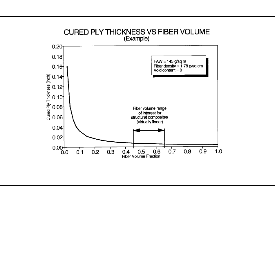
MIL-HDBK-17-1F

Volume 1, Chapter 2 Guidelines for Property Testing of Composites

2-72

thickness (and hence cured ply thickness) is also dependent only upon resin content. Thus, it follows that

cured ply thickness is solely dependent upon fiber volume fraction for constant fiber areal weight and void

content. This dependency permits normalization of each individual test specimen by its ply thickness (to-

tal thickness divided by number of plies). An example of this relationship between cured ply thickness

and fiber volume fraction (which is virtually linear within the 0.45 to 0.65 fiber volume fraction range of

usual interest for structural composites) is shown in Figure 2.4.3.2.

The following describes the derivation of an equation for normalizing each individual test specimen.

Using the relationships discussed in the previous paragraph, expressions for

normalizing

and FV

specimen

are

developed and substituted into Equation 2.4.3.2(a). For illustrative simplicity compatible units of measure

are assumed.

The first step is to define an equivalent thickness of fiber which would result if the fiber material could

be shaped into a solid sheet of uniform thickness with no air space between filaments:

FAW

2.4.3.2(b)

FIGURE 2.4.3.2 Example of correlation of cured ply thickness with fiber volume fraction.

where

= equivalent thickness of a solid layer of fiber

FAW = reinforcement fiber areal weight

= fiber density

The fraction of fiber in a laminate is then the thickness of this fiber layer divided by the total laminate

thickness:

FV =

CPT

`2.4.3.2(c)

where

FV = fiber volume fraction

MIL-HDBK-17-1F

Volume 1, Chapter 2 Guidelines for Property Testing of Composites

2-73

CPT = laminate cured ply thickness

From Equations 2.4.3.2(b) and 2.4.3.2(c) it follows that

FV =

FAW

xCPT

2.4.3.2(d)

This is the equation that was plotted for the example in Figure 2.4.3.2. It then follows that

normalizing

nominal

normalizing

FAW

CPT

2.4.3.2(e)

and

specimen

FAW

CPT

2.4.3.2(f)

where

normalizing

= fiber volume fraction specified or chosen for normalizing

specimen

= fiber volume fraction of the specimen

FAW

nominal

= nominal fiber areal weight from a material specification or other source

FAW

specimen

= specimen actual fiber areal weight

CPT

normalizing

= cured ply thickness corresponding to normalizing fiber volume fraction

CPT

specimen

= actual specimen ply thickness (specimen thickness divided by number of plies)

Combining Equations 2.4.3.2(e) and 2.4.3.2(f), the following is obtained:

normalizing

specimen

nominal

specimen

normalizing

FAW

CPT

2.4.3.2(g)

and substituting 2.4.3.2(g) into 2.4.3.2(a) produces:

Normalized value = Test value x

FAW

CPT

nominal

specimen

normalizing

2.4.3.2(h)

Thus, each specimen can be normalized by multiplying the test value by the ratios of fiber areal weight

and cured ply thickness shown. The normalizing cured ply thickness is calculated by rearranging Equa-

tion 2.4.3.2(e) as follows:

normalizing

nominal

normalizing

CPT

FAW

2.4.3.2(i)

While Equation 2.4.3.2(h) is illustrative of the model initiated in Equation 2.4.3.2(a), it is not necessary to

calculate

CPT

normalizing

if Equation 2.4.3.2(h) is transformed to:

Normalized value = Test value x

CPT

FAW

normalizing specimen

specimen

2.4.3.2(j)

The value for

FAW

specimen

is defined as the actual fiber areal weight for each individual specimen, but

this measurement is not made on a specimen basis. However, since fiber areal weight does not usually

vary greatly within a batch of material, the batch average (or roll average, if available) fiber areal weight is

generally sufficient for normalization. In the case of laminates made by resin transfer molding (RTM) or

other non-prepreg processes, lot or roll average areal weights for the fabric or preforms should be used.

With this assumption that batch fiber areal weight approximates specimen fiber areal weight within a

batch, Equation 2.4.3.2(j) becomes:

Normalized value = Test value x

CPT

FAW

normalizing specimen

batch

2.4.3.2(k)

In actual practice, fiber areal weight is commonly reported in g/m

and fiber density in g/cm

, while ply

thickness may be in inches or millimeters. For these units, Equation 2.4.3.2(k) requires a conversion fac-

tor of 25,400 in the numerator if ply thickness is in inches, or a factor of 1000 if in millimeters. With these

factors included, Equation 2.4.3.2(k) becomes:

Normalized value = Test value x

25,400x

CPT

FAW

normalizing specimen

batch

2.4.3.2(l)

MIL-HDBK-17-1F

Volume 1, Chapter 2 Guidelines for Property Testing of Composites

2-74

Normalized value = Test value x

1000x

CPT

FAW

normalizing specimen

batch

2.4.3.2(m)

where

normalizing

= fiber volume fraction specified or chosen for normalizing

CPT

specimen

= actual specimen ply thickness (specimen thickness divided by number of

plies), inch (Equation 2.4.3.2(l)) or mm (Equation 2.4.3.2(m))

= fiber density, g/cm

FAW

batch

= batch average fiber areal weight, g/m

As stated earlier, void content affects fiber volume fraction. If porosity is "added" to a laminate, the

thickness will increase and the fiber volume fraction will decrease. However, for a given fiber areal

weight, the change in fiber volume fraction will be the same regardless of the source of a thickness

change (resin content change or void content change). Thus, when normalizing using Equation 2.4.3.2(l)

or 2.4.3.2(m), there is no need to make any adjustment for void volume. This assumes, of course, that

the void content is not so large or localized that basic load carrying capability is reduced.

A hybrid method uses both individual specimen thickness and fiber volume data obtained by experi-

mental methods (matrix digestion, ignition, optical techniques, etc.). This approach is shown by Equation

2.4.3.2(n):

Normalized value = Test value x

CPT

specimen

batchavg.

normalizing

batchavg.

2.4.3.2(n)

where

CPT

specimen

= actual specimen ply thickness (specimen thickness divided by number of

plies)

CPT

batch avg.

= batch average cured ply thickness calculated from a number of panel or

specimen thickness measurements

normalizing

= fiber volume fraction specified or chosen for normalizing

batch avg.

= batch average fiber volume fraction calculated from a number of experimental

fiber volume determinations from panels within the batch

In Equation 2.4.3.2(n), the test value is first adjusted by specimen ply thickness to an average batch ply

thickness. This essentially normalizes the data to a common fiber volume fraction, presumably the batch

average fiber volume fraction. The second ratio in Equation 2.4.3.2(n) then makes a further adjustment

from the batch average fiber volume fraction to the normalizing fiber volume fraction. This method can be

useful when fiber areal weights are not available. However, this approach requires another assumption:

that the specimens used to experimentally determine batch average fiber volume fraction had an average

ply thickness equal to

CPT

batch avg.

. This is not generally the case, since batch average cured ply thickness

may be determined from many measurements over a number of panels, while batch average fiber volume

fraction may be obtained from comparatively few specimens. If fiber volume specimens are selected

carefully so they are representative of batch ply thickness, this method may be used successfully.

2.4.3.3 Practical application of normalization

Common practice is to normalize fiber-dominated lamina and laminate strengths (both unnotched and

notched) and moduli for laminates fabricated from tapes, fabrics, and rovings. Although fiber volume ef-

fects on various matrix-dominated properties (in-plane and interlaminar shear, for example) have been

observed, there is no clear model for these effects, and such properties are not normalized. In Volume 2

of this Handbook, normalized values are presented for all mechanical strength and stiffness properties

except: 90° (transverse) tension and compression of unidirectional laminates, interlaminar (

3- or

z-direction) tension, interlaminar shear, in-plane shear, short beam strength, bearing, bearing/bypass,

strain energy release rate, and Poisson's ratio.

MIL-HDBK-17-1F

Volume 1, Chapter 2 Guidelines for Property Testing of Composites

2-75

Laminates fabricated from rovings and similar forms using a winding process present a unique situa-

tion relative to normalization. Such constructions do not have plies in the usual sense: the wound "ply"

thickness depends upon tow band width, wind spacing, and tow spread during winding. Since nominal

ply thickness and fiber areal weight are not directly applicable, normalization by ply thickness and fiber

areal weight is not possible. Test data for these materials must be normalized using the ratio of normaliz-

ing fiber volume fraction to the average measured panel fiber volume fraction (Equation 2.4.3.2(a)).

When fiber-dominated properties are normalized, data scatter should decrease compared to the un-

normalized values since variability due to fiber volume fraction differences is being reduced. Thus, coeffi-

cients of variation should be lower after normalization. However, this is not always observed, and there

are a number of reasons why the reduction in scatter expected from normalization is not invariably real-

ized:

1. If measured cured ply thicknesses are close to the normalizing thickness and fiber areal weight is

close to nominal, correction factors will be small, and may be nearly the same magnitude as er-

rors in measuring these quantities.

2. The mode of failure initiation may change as a function of fiber volume. As an example, meas-

ured (unnormalized) compression strength may increase as fiber volume fraction increases over

a given range. However, at some point additional fiber may not increase strength because the

ability of the matrix to support the fibers has been exceeded, and a stability failure occurs on a

macro scale. In this case, the relationship between strength and fiber volume breaks down, and

data scatter is not necessarily reduced by normalization.

3. Flaws in test specimens might cause premature failures. If some specimens fail because of flaws

and others at the true material limit, results of normalization will not be predictable.

4. If the coefficient of variation is already small (less than 3%, for example), further reduction as a

result of normalization should not be expected, since this level of variability is about the minimum

usually observed for most composite properties.

No change in data scatter after normalization is usually not a cause for concern. However, if data scatter

increases significantly after normalization, the reason should be investigated.

2.4.4 Dispositioning of Outlier Data

Detection of outlier data points (observations which are much lower or much higher than other obser-

vations in a data set) is part of statistical analysis and is discussed in Volume 1, Section 8.3.3. Although

Section 8.3.3 cautions against discarding outlier data for which no clear cause for its erroneous nature

has been found, there are cases where outliers can (and should) be removed based on judgment. The

following paragraphs attempt to attach some degree of structure to the judgment process so that outliers

that should be retained are not casually discarded, and those which should be deleted are not retained.

For purposes of this discussion, it is assumed that the objective of testing is to characterize the prop-

erties of a material when processed, conditioned, and tested in accordance with specified procedures and

parameters. If this is the case, variability within the test data should (ideally) reflect only material variabil-

ity (raw material quality, constituent process variability, mix ratios, etc.), processing parameter variability

(within the control ranges for the specimen fabrication process), variability in the environmental history of

the specimens prior to test (within control limits), and variability within the tolerances of the test machine

parameters. In reality there is also unavoidable random variability due to unknown and uncontrollable

factors. However, beyond these inevitable and acceptable sources of variability are sources of error that

inflate the observed data scatter. This additional variability may be due to inferior fabrication practices,

process parameters that exceed allowed control limits, test fixture or test machine deficiencies, and any

number of other factors both detectable and undetectable. The task in dealing with outlier data is to de-

termine (based on physical evidence and judgment) whether the data variability is from a source that re-

MIL-HDBK-17-1F

Volume 1, Chapter 2 Guidelines for Property Testing of Composites

2-76

flects accepted material and process variability (in which case the outlier data is retained), or from an er-

roneous external source (in which case the outlier data is discarded).

When outlier data is detected (either by visual inspection of the data or by statistical tests), the first

action should be to identify the cause through physical evidence. The following list gives some examples

of conditions that could be used as the basis for discarding outlier data (the list is not exhaustive):

1. The material (or a constituent) was out of specification

2. One or more panel or specimen fabrication parameters were outside the specified tolerance range

3. Test specimen dimensions or orientation were outside the specified tolerance range

4. A defect (not under study) was detected in the test specimen

5. An error was made in the specimen preconditioning (or conditioning parameters were out of specified

tolerance ranges)

6. The test machine and/or test fixture was improperly set up in some specific and identifiable manner

7. The test specimen was improperly installed in the test fixture in some specific and identifiable manner

8. Test parameters (speed, test temperature, etc.) were outside the specified range

9. The test specimen slipped in the grips during test

10. The test specimen failed in a mode other than the mode under test (loss of tabs, unintended bending,

failure outside the gage section, etc.)

11. A test was purposely run to verify conditions suspected to have produced outlier data

12. Data were improperly normalized

Once the search for physical causes has been completed without success, the judgment process begins.

There are many approaches to assessing outlier data for which no physical cause has been identified.

The following is suggested as one possible process, and follows the flow chart shown in Figure 2.4.4.

When an outlier is detected, it may or may not be a cause of concern. If its inclusion in the data does

not significantly affect calculated basis values and does not raise other engineering issues, it may simply

be retained without further consideration.

If an outlier data point was detected in a single batch or set of data, and if additional data sets are

available (same fabrication, conditioning, and test conditions), there are a number of considerations that

can be used to support a judgment call. If, on the other hand, additional data sets are not available, or if

the outlier was detected only after combining (pooling) several data sets (see Volume 1, Section 8.3.1),

there are fewer options to consider and judgment is more subjective.

In the case of a single data set outlier where additional data sets are available, the first consideration

is to determine if the outlier in question is within the range of the non-outliers of the other data set(s). If it

is within the non-outlier range of the other data, it is recommended that the outlier be retained.

If a single data set outlier is outside of the non-outlier range of other data, the next option is to obtain

retest data using specimens from the same part or panel as the original data that contained the outlier. If

the retest data refutes the outlier data, the retest data set may be used to replace the entire original data

set. The replacement set is then combined with the other data sets. If outliers still exist in the retest data,

the original data is retained and combined with the other data sets. The retest data set may also be

added to the body of data. Regardless of whether the original data was replaced or not, the combined set

is then tested for outliers. If no outliers are detected in the combined set of data, no deletions from the

combined set are made.

MIL-HDBK-17-1F

Volume 1, Chapter 2 Guidelines for Property Testing of Composites

2-77

Single

batch

outlier before

pooling ?

Other

batches

Available?

High

outlier?

Original

panel or part

available?

Does

retest data

refute outlier?

Within

range of

other batch

non-outliers

Start

yes

Far beyond

material

capability?

Outlier may

be discarded

yes

Outlier should

be retained

yes

Run retests on

same panel or part

Combine set with

other sets (batches)

Still an

Outlier?

yes

Replace entire original

data set with retest data

no no

Add retest data set

there an

engineering

concern?

yes

FIGURE 2.4.4 Judgment process for dispositioning of outlier data without identified cause.

MIL-HDBK-17-1F

Volume 1, Chapter 2 Guidelines for Property Testing of Composites

2-78

If there are outliers in the combined data set (or in a single set where no additional sets were avail-

able), the judgment process becomes even more subjective. In this case it is recommended that only

high outliers be considered for deletion. Generally, if a high outlier is so high that, based on experience

and similar test results from other sources, it is clearly beyond the known or expected capability of the

material, it may be discarded. If low outliers exist in single data sets and no additional sets are available,

additional batches should be tested and the judgment process repeated. Retests of the same single

batch are not considered sufficient without additional batch information.

Note that the judgment process does not specifically identify a cause, and does not really prove that

the questionable data resulted from erroneous variability. The judgment process attempts to build a body

of information that leads to the conclusion that it is highly likely that erroneous variability (caused by

something other than expected material, process, or testing variations) was responsible for the outlier.

This approach to outlier disposition should only be used after all attempts to identify and quantify physical

causes have failed. The rationale for any data deletions made by the judgment process should be fully

documented.

2.4.5 Data documentation

This section is reserved for future use.

2.5 MATERIAL TESTING FOR SUBMISSION OF DATA TO MIL-HDBK-17

2.5.1 Introduction

Section 2.5 describes the requirements for publication of material property data in MIL-HDBK-17 Vol-

ume 2. A Data Source Information Package is available from the MIL-HDBK-17 Coordinator or Secre-

tariat to aid data suppliers in submitting data to the Handbook. This package provides recommendations

on data preparation and transfer and a diskette containing ASCII text and spreadsheet files containing

suggested formats for specimen, batch, and material information. The overall data submittal and review

process is described in Section 1.5 and summarized in Figure 2.5.1.

Material property data sets submitted for possible publication are classified by one of the MIL-HDBK-

17 data classes described below, and are examined to see that material and process (Section 2.5.2),

sampling (Section 2.5.3), conditioning (Section 2.5.4), test methods (Section 2.5.5), and data documenta-

tion (Section 2.5.6) requirements are met for the properties discussed in Sections 2.5.7-2.5.11. B-basis

values are presented in the handbook only for B and A data classes. (If sufficient data are available, an A

class designation is used and both A- and B-values are presented). The MIL-HDBK-17 data classes are:

• A75 – Robust Sampling Data

Statistically-based material properties that meet the most stringent handbook level of population

sampling, data documentation and test method requirements. A- and B-values are presented in the

handbook. The upper-case letter A is used for summary tables.

• A55 – Reduced Sampling Data

Statistically-based material properties that meet the most stringent handbook level of data documen-

tation and test method requirements with reduced sampling appropriate for certain applications (See

Volume 3, Chapter 4, [Building Block Approach]). A- and B-values are presented in the handbook.

The lower-case letter a is used for summary tables.

MIL-HDBK-17-1F

Volume 1, Chapter 2 Guidelines for Property Testing of Composites

2-79

FIGURE 2.5.1 Data submittal and review process.

• B30 – Robust Sampling Data

Statistically-based material properties that meet the most stringent handbook level of population

sampling for B-values, data documentation and test method requirements. B-values are presented in

the handbook. The upper-case letter B is used for summary tables.

The B30 data class corresponds to the Fully Approved class in MIL-HDBK-17 versions B through E.

MIL-HDBK-17-1F

Volume 1, Chapter 2 Guidelines for Property Testing of Composites

2-80

• B18 – Reduced Sampling Data

Statistically-based material properties that meet the most stringent handbook level of data documen-

tation and test method requirements with reduced sampling appropriate for B-values for certain appli-

cations (See Volume 3, Chapter 4 (Building Block Approach)). B-values are presented in the hand-

book. The lower-case letter b is used for summary tables.

• M – Mean Data

Mean material properties that meet the most stringent handbook level of data documentation and test

method requirements. This data class generally applies to modulus and Poisson’s ratio data and

other properties for which basis values are not typically used. The upper case letter M is used for

summary tables.

• I – Interim Data

Data that do not meet the specific sampling or data documentation requirements required of B and A

data classes. Interim data can be subdivided into two categories:

1. Data that meet data documentation requirements for B and A data classes, but for which insuffi-

cient batches or replicates were tested. These data may potentially be pooled with other data to

create a properly-sampled population that meets the B and A data requirements.

2. Data which fail to meet the data documentation requirements for B and A data, even if the popula-

tion sampling is adequate for those data classes. Such data cannot be used for subsequent pool-

ing.

• S – Screening Data

Data representing fewer than three batches, or data resulting from a test method limited to the

screening level of approval. The screening data class is intended to provide for rapid inclusion in the

handbook of data for new materials and other information that is useful even with a limited data set as

described in Section 2.1.2.2 and as illustrated by the recommended test matrix of Table 2.3.1.1.

Note that, for uses other than inclusion in MIL-HDBK-17, selection of a material data class for use in an

application is subject to agreement between the contractor and the certifying agency.

2.5.2 Material and process specification requirements

All materials submitted to the handbook should be manufactured in accordance with a material speci-

fication that imposes requirements on key physical and mechanical properties and should be processed

in accordance with a process specification that adequately controls key processing parameters.

2.5.3 Sampling requirements

As noted in Section 2.2.5.1, the magnitude of a basis value is a function of the amount of data ob-

tained, the number of batches represented, and the uniformity of the batches produced. Basis values are

presented in the handbook only for B and A data classes. The minimum sampling requirements for each

class are shown in Table 2.5.3.

The essence of documentation requirements is complete traceability and control of the database de-

velopment process from material production, through procurement, fabrication, machining, environmental

conditioning, gaging, testing, data acquisition, data normalization, and final statistical interpretation. The

key items of information from this process for lamina/laminate mechanical testing are summarized in Ta-

ble 2.5.6 and should be documented as part of any such material property determination. The items

marked (

•) should be included with any data submitted to the Secretariat. The items marked (⊗), as well

as all items marked (

•), must be included in the submission in order for submitted data to qualify for B, A,

and M data classes. All other information should be traceable and available to the Secretariat for valida-

tion of statistical outliers. This list is based on the information necessary for lamina/laminate level me-

MIL-HDBK-17-1F

Volume 1, Chapter 2 Guidelines for Property Testing of Composites

2-81

chanical property testing. Individual documentation items or documentation groups are not required

where they are not applicable

TABLE 2.5.3. Minimum sampling requirements for MIL-HDBK-17 data classes.

Minimum Requirements

Designation

Symbol

Description

Number of

Batches

Number of

Specimens

A75 A A-Basis – Robust

Sampling

10 75

A55 a A-Basis – Reduced

Sampling

5 55

B30 B B-Basis – Robust

Sampling

5 30

B18 b B-Basis – Reduced

Sampling

3 18

M M Mean 3 18

I I Interim 3 15

S S Screening 1 5

2.5.3.1 Additional requirements for B and A data classes

The prepreg batches should be prepared by the material supplier using production facilities. The first

prepreg batches, up to five, should each be made using distinct fiber and matrix constituent lots (not re-

quired for batch numbers greater than five). For each condition and property, batch replicates should be

sampled from at least two different test panels covering at least two separate processing cycles. Test

panels should be nondestructively evaluated using ultrasonic inspection or another suitable nondestruc-

tive inspection technique. Test specimens should not be extracted from panel areas having indications of

questionable quality. A test plan (or report) should document laminate design, specimen sampling details,

fabrication procedures (including material traceability information), inspection methods, specimen extrac-

tion methods, labeling schemes, and test methods.

2.5.3.2 Data pooling

The ability to pool multiple similar but not identical data sets is desirable in order to obtain sufficient

data to calculate material property basis values. Data sets for pooling may be available for materials from

different fabricators, different locations of a single fabricator, or slightly different processes from the same

fabricator.

Decisions on suitability of pooling will be made by the MIL-HDBK-17 Data Review working group,

which will examine all tested properties for batch-to-batch variability (Section 8.3.2.2). Advance approval

of the MIL-HDBK-17 Data Review working group is recommended before starting a new testing program

that relies on pooling. However, MIL-HDBK-17 Data Review approval of a specific pooling process will

not guarantee that the material data sets will, when testing is completed, be found to be poolable. Pre-

liminary investigations into poolability are recommended before committing significant resources to

large-scale testing.

For example, fastener type and torque-up conditions are applicable to the bolt-bearing test but not to a tension test. Consequently,

the reporting of this information is required for the bearing test and is not required for the tension test.

MIL-HDBK-17-1F

Volume 1, Chapter 2 Guidelines for Property Testing of Composites

2-82

MIL-HDBK-17 Data Review has already pre-approved a pooling process for the case when several

different fabricators wish to jointly develop B-basis data for MIL-HDBK-17 submission. Standard material

and process specifications must be used and available. Sampling requirements are a minimum of three

fabricators, each producing panels from at least three different batches of material. The minimum of nine

batches must be sampled from five distinct prepreg batches, as discussed in Section 2.5.3.3. The batch

replicate, processing, inspection, planning, and reporting requirements of Section 2.5.3.3 also hold.

2.5.4 Conditioning requirements

This section is reserved for future use.

2.5.5 Test method requirements

Specific test method criteria apply when submitting data to MIL-HDBK-17 for consideration for inclu-

sion in Volume 2 of the Handbook, based on the following concepts. Ideally, a test method should have

undergone a rigorous review of its applicability, precision and bias by an independent voluntary consen-

sus standards organization that may include representatives from material suppliers, end-users, acade-

mia, or government. This review, and the test method, should be available in a referenceable, open-

literature publication, and include interlaboratory (round robin) testing. Many times test methods meeting

the above criteria are not available, and methods which meet less rigorous criteria (2 or 3 below) must be

selected for data submittal.

The MIL-HDBK-17 Coordination Group has identified specific test methods, based on the material’s

structural complexity level (Section 2.1.2.1) and property, to be used when submitting data for considera-

tion for inclusion in Volume 2 of the Handbook. These methods are designated or described in Chapters

3 through 7, and meet one or more of the following criteria:

1. Methods, applicable to advanced composites and in common use, which have completed the fol-

lowing:

• Round robin testing under sponsorship of a recognized standards-making organization

• Rigorous review of precision and bias

• Publication in the open literature of a recognized standards-making organization

2. "Common practice" methods, which have not been standardized as in (1) above, but which are in

common usage in the composite materials industry, are available in referenceable, open-literature

publications, and have begun the process toward formal standardization.

3. Where no standards meeting the above criteria exist for specific structures or process/product

forms, other test methods may have been selected by consensus of the MIL-HDBK-17 Coordina-

tion Group. Such methods may have been developed within the MIL-HDBK-17 Working Groups,

or by other organizations, and will have begun the process toward formal standardization.

The test methods used for data submittal to the handbook must meet the handbook recommendations,

summarized in Table 2.2.4, at the time the tests were performed. Fully Approved test methods are re-

quired for B and A data classes. Interim test methods are acceptable for I class data and Screening test

methods are acceptable for S class data.

2.5.6 Data documentation requirements

This section outlines data documentation requirements necessary for the inclusion of data in

MIL-HDBK-17 Volume 2. Data must meet the data documentation requirements that are in effect on the

date of submission to the handbook. The data documentation requirements in effect at the time of publi-

cation of the handbook are provided in Table 2.5.6. Note that these requirements are subject to subse-

quent modification and that the latest authoritative data documentation requirements, which may differ

slightly from Table 2.5.6, must be obtained from either the Secretariat or the Coordinator.

MIL-HDBK-17-1F

Volume 1, Chapter 2 Guidelines for Property Testing of Composites

2-83

TABLE 2.5.6 Documentation requirements

Material identification - required for all composite materials

material identification

material class (e.g., C/EP)

▼

material procurement specification

Matrix material - required for all composite materials

commercial designation

manufacturer

date of manufacture, earliest and latest

lot number for each lot

nominal density and test method

Reinforcement - required for all composite materials

precursor type (i.e., PAN, Rayon)

commercial designation

manufacturer

date of manufacture, minimum and maximum

lot number for each lot

surface treatment (Y/N)

▼

surface treatment type

surface finish (sizing) identification and amount

density (average per lot) and test method

nominal filament count

twist

Preform

preform architecture

preform identifier

preform manufacturer

preform method of manufacture - molded, stitched, RFI, etc.

number of preform layers

2-D Fabric

▼

fabric manufacturer/weaver

fabric family (weave pattern)

fabric standard style number (particularly for glass fabrics)

fabric sizing identification

fabric sizing content

fabric warp and fill tow count per inch

fiber areal weight per batch

fabric fill fiber (if different)

3-D Woven Materials (including triaxial fabric)

interlock description

warp fiber filament count

weft fiber filament count

angle fiber filament count

weaver yarn filament count

percentage of warp yarn

percentage of weft yarn

angle of angle yarn (positive with respect to axial yarn)

percentage of angle yarn

percentage of weaver yarn

See Part Description, fiber areal weight

MIL-HDBK-17-1F

Volume 1, Chapter 2 Guidelines for Property Testing of Composites

2-84

percentage of through-thickness yarn

pitch length

warp end count

weft end count

Stitching Information

stitch type

stitch thread

stitch axial pitch

stitch row spacing

▼

stitch denier

stitch filament count

bias yarn end count

bias yarn angle

Braiding Information

braid description

axial fiber type

braid fiber type

axial fiber filament count

braid fiber filament count

braid angle

percentage of axial yarn

percentage of braid yarn

▼

axial yarn spacing in braids

Winding Description

winding description

Prepreg

ply manufacturer

date of manufacture

material lot number

commercial designation

material form - tape/fabric

fiber areal weight per batch

total resin content per lot

▼

volatile content

scrim material class

scrim fabric style

Processing - required for all composite materials

▼

process specification

lay-up schematic (including bagging, scrim, bleeder, etc.)

⊗

part manufacturer

date of manufacture (date completed)

reinforcement application process (how the fiber/preform was put together) - see Volume 2, Table

1.4.2(b)

cure process type (how the part was cured/molded) - see Volume 2, Table 1.4.2(b)

▼

tackifier common name

▼

tackifier material class (e.g., epoxy)

▼

tackifier form - aerosol/liquid

▼

tackifier manufacturer

See Part Description, fiber areal weight

MIL-HDBK-17-1F

Volume 1, Chapter 2 Guidelines for Property Testing of Composites

2-85

Process Description - appropriate group required for all composite materials

Autoclave/oven/press cure

near-net or extra resin process

temperature for putting uncured part into autoclave/oven/press (including range)

ramp rate to cure conditions

cure conditions - temperature, pressure, duration,

ramp rate to postcure

postcure conditions - temperature, pressure, duration,

cooling rate

part removal temperature

other critical control parameters

RTM (not applicable to RFI)

degas steps on the resin prior to injection

initial tool temperature

preform insertion temperature

heat-up rate, soak time and temperature before injection

vacuum used (Y/N) and inches Hg

injection rate (cm

/min), temperature, and pressure

cure temperature, pressure, and duration

cooling rate and part removal temperature

additional postcure (Y/N) - temperature, duration, in-tool/free-standing

Part Description- required for all composite materials

form (panel, tube, etc.)

ply count

lay-up code

fiber areal weight

, nominal, by batch or part, and test method

nominal fiber volume

and test method

▼

resin content (weight or volume), nominal and test method

⊗

void content, nominal, by batch or part, and test method

density, nominal, by batch or part, and test method

ply thickness, nominal, by batch or part, and test method

glass transition temperature (wet and dry, nominal) and test method

Specimen preparation- required for all composite materials

specimen orientation

⊗

tab adhesive curing temperature (nominal)

Mechanical testing- required for mechanical testing of all composite materials

number of specimens

test procedure (citing all deviations from standard procedures including reporting requirements. It is

assumed that, other than the deviations reported, the test method was followed.)

date of applicable standard

date of testing

specimen thickness for each specimen

specimen conditioning standard method

conditioning temperature

conditioning humidity

conditioning time

conditioning environment (if not lab air), standard designation of fluids if available

Fiber volume or fiber areal weight (FAW) for each batch or panel is required. For prepregs, batch or roll average FAW is accept-

able. For other materials, lot or roll average FAW of the assembled reinforcement (fabric, braid, or preform) is acceptable. If addi-

tional out-of-plane reinforcement, such as stitching is used, the lot or roll average FAW can be obtained for the reinforcement as-

sembly prior to the out-of-plane reinforcement (e.g., unstitched fabric).

If multi-step conditioning method was used, provide conditioning information for each step.

MIL-HDBK-17-1F

Volume 1, Chapter 2 Guidelines for Property Testing of Composites

2-86

equilibrium (Y/N)

⊗

moisture content, specify whether moisture content or uptake

test temperature

soak time at test conditions prior to load initiation

fastener type and torque-up conditions (bearing, mechanically fastened joint (MFJ), filled hole)

hole diameter (open/filled hole, bearing, MFJ)

▼

hole clearance, countersink angle and depth (filled hole, bearing, MFJ)

nominal thickness, width, and material for each member (bearing, MFJ)

edge distance (bearing, MFJ)

fixture torque-up (e.g., SACMA RM-1)

shear strain at which test was truncated (shear)

failure mode identification and location

all non-normalized (raw) data

method of calculating modulus and Poisson's ratio

method of finding offset strength (bearing)

method of finding proportional limit (bearing

method of calculating fracture toughness (fracture toughness)

method of finding proportional limit (bearing)

method of calculating fracture toughness (fracture toughness)

z Required for submission to Secretariat

⊗ Required submission to the Secretariat for B and A data classes

▼ Requested for submission to the Secretariat, presented if available

General recommendations on data documentation are provided in Section 2.2.12. The essence of

documentation requirements is complete traceability and control of the database development process

from material production, through procurement, fabrication, machining, environmental conditioning, gag-

ing, testing, data acquisition, data normalization, and final statistical interpretation. The key items of in-

formation for mechanical testing of composite materials are summarized in Table 2.5.6 and should be

documented as part of any such material property determination. The items marked (z) should be in-

cluded with any data submitted to the Secretariat. The items marked (

⊗), as well as all items marked (z),

must be included in the submission in order for submitted data to qualify for B and A data classes. Items

marked (▼) are requested for submission to the Secretariat; this information will be presented in Volume 2

if available. Recommendations for in-house documentation are discussed in Volume 1, Section 2.2.12.

All reasonable information should be traceable and available to the Secretariat for validation of statistical

outliers.

This list is based on the information necessary for mechanical property testing. The documentation

requirements are grouped by possible forms at various stages of fabrication. Groups required for all com-

posite materials are identified. Material Identification, Matrix Material, and Reinforcement groups are re-

quired for all types of materials. The items in the Preform and Prepreg groups are required based on ad-

ditional steps in fabricating the material as indicated for each fabrication form. For example, a (2-D) fabric

prepreg would require the 2-D Fabric portion of the Preform group and the Prepreg group. The appropri-

ate section within Process Description should be used. The remaining groups apply to all mechanical

property testing. Note that items are grouped by whether or not they are needed to include relevant in-

formation for a particular stage of fabrication. For most items, this also is the fabrication form from which

the information is obtained. There are a few exceptions to the latter grouping. For example, information

on scrim is included with Prepreg since that is the form which requires scrim information. Fiber areal

weight should be measured at the most appropriate stage of fabrication. Individual documentation items

are not required where they are not applicable

For example, fastener type and torque-up conditions are applicable to the bolt-bearing test but not to a tension test. Consequently,

the reporting of this information is required for the bearing test and is not required for the tension test.

MIL-HDBK-17-1F

Volume 1, Chapter 2 Guidelines for Property Testing of Composites

2-87

The information required for other types of tests or material levels is similar. For instance, prepreg

property testing would require the prepreg, reinforcement, matrix, and possibly fabric information, as well

as appropriate information on specimen preparation and testing procedures.

2.5.7 Data normalization

Certain types of data should be normalized to provide consistent presentation of properties and to

allow for reasonable material comparison. For mechanical properties, data are normalized by the Secre-

tariat for lamina/laminate strength and stiffness properties except 90° (transverse) tension and compres-

sion of unidirectional laminates, interlaminar (

3- or z-direction) tension, interlaminar compression, inter-

laminar shear, in-plane shear, short beam strength, bearing and bearing/bypass, strain energy release

rate, and Poisson's ratio. The procedures from Section 2.4.3 should be used for normalization of hand-

book mechanical data, in the following order of preference:

1. By fiber volume as measured on the test specimen as shown in Equation 2.4.3.2(a),

2. By specimen cured ply thickness and batch average fiber areal weight as shown in Equation

2.4.3.2(k)

3. By specimen cured ply thickness and batch average fiber volume as shown in Equation 2.4.3.2(n)

Data for unidirectional tape are normalized to 60% fiber volume and data for fabric are normalized to 57%

fiber volume unless another value is considered more appropriate by the Data Review working group.

Normalization procedures for other properties have not yet been approved.

2.5.8 Statistical analysis

All data for the handbook are analyzed according to the flowchart in Section 8.3.1. Where batch-to-

batch variability can be neglected (based on Section 8.3.2) the data model used is the first data model

with an observed significance level greater than 0.05. Models are considered in the following order -

Weibull, normal, lognormal, and nonparametric. Selection of statistical approach including consideration

of pooling (Section 2.5.3) is subject to review and approval by the Data Review working group.

2.5.9 Mechanical properties of laminae and laminates

Handbook values for mechanical properties of each material will be listed in the data summary in Vol-

ume 2.

2.5.9.1 Unidirectional properties from laminates

A laminate "backing-out" approach for unidirectional material lamina mechanical properties is docu-

mented in Section 2.4.2. Data by this approach will be considered for inclusion in the handbook accord-

ing to the procedures in Figure 2.5.1. While the Section 2.4.2 approach is applicable to many lay-ups and

other possibilities continue to be explored, to date only [90/0]ns laminates have been considered accept-

able by the MIL-HDBK-17 Coordination Group.

2.5.9.2 Strength and strain-to-failure

Handbook values for strength, and strain-to-failure should meet the sampling requirements in Section

2.5.3 for each property and at each condition. For the data to be included in the population, failure modes

must be considered acceptable in accordance with the test method used. Strengths will be normalized

according to Sections 2.4.3 and 2.5.7. Strengths and strains-to-failure will receive the full statistical

treatment described in Section 8.3.1 including outlier detection, data pooling testing, determination of dis-

tribution, and B-basis value calculation.

MIL-HDBK-17-1F

Volume 1, Chapter 2 Guidelines for Property Testing of Composites

2-88

2.5.9.3 Elastic moduli, Poisson's ratios, and stress/strain curves

Handbook values for elastic moduli (Young's moduli or shear moduli) and Poisson's ratios, calculated

over a fixed strain range, should meet the sampling requirements in Section 2.5.3 for each property and

at each condition. The elastic moduli should be normalized according to Sections 2.4.3 and 2.5.7 and all

results receive the statistical analysis outlined in Section 8.3.1. Minimum, average, maximum, and coeffi-

cient of variation (CV) values will be tabulated for moduli, and the average value tabulated for Poisson's

ratio. The report should include the calculation method and strain ranges for each property. If

stress/strain data are provided an average stress/strain curve will be calculated using the procedures de-

scribed in Section 8.4.4 and reported as shown in Volume 2, Section 1.4.2.

2.5.10 Chemical properties

This section is reserved for future use.

2.5.11 Physical properties of laminae and laminates

Handbook values for physical properties (at 73±5°F (23±3°C), if available) will be listed in the data

summary for each material. Additional values as a function of temperature or other parameters, if avail-

able, will be presented graphically.

2.5.11.1 Density

The handbook value for density should be determined at a specified temperature (in the absence of a

specific requirement use 73±5°F (23±3°C)) from the average of a minimum of three specimens for each

batch used in the determination of any mechanical properties.

2.5.11.2 Composition

This section is reserved for future use.

2.5.11.3 Equilibrium moisture content

Handbook values for equilibrium moisture content should be determined for specified relative humid-

ity and temperature values (in the absence of a specific requirement, use 85%RH, 180°F (82°C)) from the

average of a minimum of three specimens at each condition. If additional information is available for

equilibrium moisture content as a function of temperature and relative humidity, those values will be pre-

sented graphically.

2.5.11.4 Moisture diffusivity

Handbook values for moisture diffusivity should be determined for specified temperatures (in the ab-

sence of a specific requirement use 180°F (82°C)) from the average of a minimum of three specimens at

each temperature. If additional information is available for moisture diffusivity as a function of tempera-

ture and relative humidity, those values will be presented graphically.

2.5.11.5 Coefficient of moisture expansion

Handbook values for moisture expansion coefficient should be obtained and will be reported in the

same way as those for thermal expansion coefficient (Section 2.5.12.1).

2.5.11.6 Glass transition temperature

Handbook values for glass transition temperature should be determined for dry and wet material con-

ditions from the average of a minimum of three specimens at each condition. Guidelines for glass transi-

tion temperature testing and maintenance of a wet condition are discussed in Section 6.4.3.

MIL-HDBK-17-1F

Volume 1, Chapter 2 Guidelines for Property Testing of Composites

2-89

2.5.12 Thermal properties

Thermal property room temperature values will be listed in the data summary. Additional values as a

function of temperature, if available, will be presented graphically in a single figure according to Volume 2,

Section 1.4.3. Each property should be determined for a specified temperature or temperature range.

Default values, to be used when temperatures are not otherwise specified, are provided for different ma-

trix materials in Table 2.5.12. The room temperature default value for all materials is 73°F (23°C). The

tolerance on all default temperatures is ±5F° (±3C°).

TABLE 2.5.12 Default temperatures for handbook thermophysical data.

Matrix Material

Default Elevated

Temperature

Default Temperature

Range

Family °F °C °F °C

Epoxy 220 104 73 - 275 23 -135

Bismaleimide 350 177 73 - 450 23 - 232

PEEK 220 104 73 - 250 23 - 121

Polyimide 550 288 73 - 600 23 - 315

2.5.12.1 Coefficient of thermal expansion

Handbook values for average coefficient of linear thermal expansion (CTE) should be determined for

specified temperature ranges (in the absence of a specific requirement, use the default temperature

range for the appropriate matrix material family in Table 2.5.12) from the average of a minimum of five

specimens for each temperature range. The reference temperature for thermal expansion should be

clearly noted.

2.5.12.2 Specific heat

Handbook values for constant pressure specific heat should be determined at specified temperatures

(in the absence of a specific requirement use the room temperature default) from the average of a mini-

mum of three specimens for each temperature.

2.5.12.3 Thermal conductivity

Handbook values for average thermal conductivity should be determined for specified temperature

ranges (in the absence of a specific requirement, use the default temperature range for the appropriate

matrix material family in Table 2.5.12) from a minimum of three specimens for each temperature range.

2.5.12.4 Thermal diffusivity

Handbook values for thermal diffusivity should be determined for specified temperatures (in the ab-

sence of a specific requirement, use the default elevated temperature for the appropriate matrix material

family in Table 2.5.12 as the median temperature) from the average of a minimum of three specimens for

each temperature.

MIL-HDBK-17-1F

Volume 1, Chapter 2 Guidelines for Property Testing of Composites

2-90

2.5.13 Electrical properties

This section is reserved for future use.

2.5.14 Fatigue

Fatigue is defined as the change in property as a result of repeated mechanical loading in the appro-

priate environmental conditions. This is not normally considered a design limiting property for PMC struc-

tures that have been designed with fiber dominated lay-ups and have minimal out-of-plane loading condi-

tions. The exceptions to this generalization are high cycle fatigue components like rotor blades, propeller

blades, and engine fan blades. These structures encounter a high number of cyclic loads (up to 5x10^8)

and should not be sized for static and damage considerations alone. In these applications, fatigue is an

important property. The "building block" design/validation approach using coupon, element, and compo-

nent testing can be used to assure adequate fatigue life.

Fatigue should be addressed at various levels of development:

• Basic material property screening- Primary purpose is to compare various materials to aid in the

selection process.

• Design allowables-Purpose is to characterize the specific material selected with sufficient repli-

cate testing and conditions to ensure adequate performance of the completed design by analysis.

An additional use of this level of testing is to define fatigue enhancement factors for conducting

higher level (more complex) element and component tests.

There is no established practice of using laminae fatigue data to construct laminate fatigue allow-

ables, so it is recommended that application specific laminate based allowables be generated. ASTM

D3479, "Tension-Tension Fatigue Oriented Fiber, Resin Matrix Composites" is a generalized coupon test-

ing method that can be used as a guide for a fatigue test method. Note, this published test method ap-

proach is for tension-tension fatigue. Compression-compression and tension-compression fatigue are

typically more critical in composites.

The following are some general guidelines for specimen fatigue testing. Fatigue data is generated at

the design critical test conditions, i.e. -65F, room temperature, or hot/wet. Design critical test conditions

are very application dependent. For hot/wet testing, specimens should be brought to their desired mois-

ture level prior to testing, and maintained at this moisture level during the actual fatigue test. The desired

moisture level is again application dependent. It may be an equilibrium moisture level for a specified rela-

tive humidity, a percentage of an equilibrium level, or some other condition defined by the specific applica-

tion environment, part geometry, and projected service life. As an example, Reference 2.5.14(a)

(J. Rouchon) contains the methodology used by one certifying agency.

Like the generation of static design allowables, notches can be used for fatigue testing as well. This

approach could be non-conservative, in that a notched specimen has a greatly reduced volume of mate-

rial at the maximum stress cross-section when compared to an unnotched specimen. If the purpose of the

specimen test is to account for material and process variation effects on fatigue performance, the un-

notched specimen is a more appropriate configuration. Unnotched specimen failures will initiate at ran-

dom failure sites that are inherent in the specimen, whereas notched specimen failures are constrained to

initiate at the manufactured notch.

If the purpose of the fatigue testing is to provide a structural level assessment of process variation,

the use of actual manufacturing anomalies may be more appropriate. Composite structure based manu-

facturing anomalies, such as delaminations, disbonds, fiber breaks, are important in a cyclic load envi-

ronment because it must be shown they will not grow significantly in the no growth damage tolerance ap-

proach or they will not grow to a critical length during the life of the component or before they are de-

tected by inspection in the growth approach. Element, component, and sub-component level fatigue tests

are usually recommended to substantiate allowable manufacturing anomaly limits and also to establish

in-service inspection requirements.

MIL-HDBK-17-1F

Volume 1, Chapter 2 Guidelines for Property Testing of Composites

2-91

Fatigue data for in-plane material property performance can be evaluated with three R-ratios: R=0.1

(tension-tension), R=10.0 (compression-compression), and R=-1.0 (tension-compression). Design fatigue

loading conditions may not dictate the full spectrum of loading conditions, but with these three R-ratios a

Goodman diagram (Reference 2.5.14(b)) can be constructed to aid in predicting fatigue at any given

R-ratio. For interlaminar properties, it is recommended two R-ratios be run, R=0.1 and R=-1 .0. R=10.0 is

not necessary for flatwise (through the thickness) fatigue, since this is not typically a viable failure mode.

The loading conditions are the same for R=10.0 and R=0.1 for interlaminar shear fatigue, so R=10.0 tests

are not performed.

Tests are typically run in load control. Strain control tests are not generally necessary because of

PMC's linear elastic behavior. Unless test frequencies are set to be the same as in-service frequencies,

test frequencies should be set so that any temperature rise in the specimen is limited to 5F. Generally,

test frequencies of 5-10 hertz are used. All specimens should be thermo-coupled to ensure specimen

heating is insignificant during all fatigue testing. The use of in-service frequencies during testing can be

important, since it has been shown that increased test frequencies can increase fatigue life in some mate-

rials/test configurations.

Failure mode evaluation of fatigue test specimens are just as important as for static test specimens.

Erroneous data can be generated if an improper failure mode occurs. The typical undesirable failure

modes to avoid include, tab debonding, non-gauge section failures, and fiber splitting in geometry transi-

tion areas. Fatigue specimen design and fabrication quality are very significant in achieving the proper

gauge section failure modes in specimen fatigue tests.

Stress levels selected for testing should provide good data spacing on a semi-log fatigue stress vs.

cycles plot (S/N plot), and provide failure points in the cycle regime of interest. An example of a cycle

range for a low cycle fatigue (LCF) 40,000 cycle structure, would be to generate failure points from 10^3

to 10^5 cycles. The number of data points required per curve varies depending on its desired use. For

materials screening, 8 data points are usually sufficient to establish the fatigue performance. For design

allowables, 15 data points are recommended over three batches. Regression analysis or Sendeckyj's

method (References 2.5.14(c) and (d)) are efficient approaches for analyzing this data and establishing

B-basis and A-basis design allowable lines.

The fatigue design allowable curves can be used for two purposes. The first is to establish maximum

stress values for a specific number of cycles by using a B-basis or A-basis value. The other purpose is to

use the data distribution from the fatigue data of the critical design property to establish a load/life en-

hancement magnification factor used for element or component testing. Since only a small number of

elements or components are usually fatigue tested, the load/life of the test must be enhanced to account

for material and process scatter. Even though there are empirically based techniques to predict the life of

PMC structures, the element or component fatigue test is required for verification because of feature de-

pendent effects like ply drops and manufacturing complexities not accounted for in the specimen testing

or the design analysis. The load/life enhancement approach is outlined in the FM report (Reference

2.5.14(e)) and provides a sound statistical approach to ensure application durability with a limited number

of test articles. Load/life enhancement approach may also be used to account for environmental effects

that are difficult to reproduce in element or component tests.

As discussed previously, most fatigue concerns in composites apply to high cycle applications. Most

aircraft structure is subjected to a range of loads with various amplitudes and maxima (spectra loading).

These structures are not characteristically high cycle. The spectrum loading introduces another complex-

ity that has proved difficult to account for in life prediction. Cumulative damage approaches developed for

metallic structure have been shown to be ineffective in composites. This has necessitated an increased

reliance on empirical procedures for life verification rather than life prediction.

MIL-HDBK-17-1F

Volume 1, Chapter 2 Guidelines for Property Testing of Composites

2-92

REFERENCES

2.1.1(a) Rouchon, J., “Certification of Large Aircraft Composite Structures, Recent Progress and

New Trends in Compliance Philosophy,” presented at the 17th ICAS, Stockholm, Sweden,

1990.

2.1.1(b) Whitehead, R. S., Ritchie, G. L., and Mullineaux, J. L., "Qualification of Primary Composite

Aircraft Structures," presented at the USAF ASIP Conference, Macon, GA, 27-29 Novem-

ber, 1984.

2.1.1(c) Whitehead, R. S., and Deo, R. B., "A Building Approach to Design Verification Testing of

Primary Composite Structures," Proceedings of the 24th AIAA/ASME/AHS SDM Confer-

ence, Lake Tahoe, NV, May 1983, pp. 473-477.

2.2.4 Fields, R. E, "Improving Test Methods for Composites," ASTM Standardization News, Oct.

1993, pp. 38-43.

2.2.7(a) ASTM Test Method D 570 "Water Absorption of Plastics," Annual Book of ASTM Standards,

Vol. 8.01, American Society for Testing and Materials, West Conshohocken, PA.

2.2.7(b) ASTM Practice D 618 "Conditioning Plastics and Electrical Insulating Materials for Testing,"

Annual Book of ASTM Standards, Vol. 8.01, American Society for Testing and Materials,

West Conshohocken, PA.

2.2.7(c) ASTM Test Method D 5229/D 5229M "Moisture Absorption Properties and Equilibrium

Conditioning of Polymer Matrix Composite Materials," Annual Book of ASTM Standards,

Vol. 15.03, American Society for Testing and Materials, West Conshohocken, PA.

2.2.7(d) Ryder, J.T., “Effect of Load History on Fatigue Life”, AFWAL-TR-80-4044, July 1980.

2.2.7.1 Hedrick, I. G., and Whiteside, J. B., "Effects of Environment on Advanced Composite Struc-

tures," AIAA Conference on Aircraft Composites: Emerging Methodology for Structural As-

surance, San Diego, CA, 1977.

2.2.7.3(a) Whiteside, J. B., et al, "Environmental Sensitivity of Advanced Composites," Volume 1, En-

vironmental Definition, AFWAL-TR-80-3076.

2.2.7.3(b) MIL-STD-210C, Climatic Information to Determine Design and Test Requirements for Mili-

tary Systems and Equipment.

2.2.7.3(c) Sanger, K.B., “Certification Testing Methodology Structures”, Naval Air Development Cen-

ter Report NADC-86132-60 on Federal Aviation Administration Report DOT/FAA/CT-36/38,

Jan 1986, p. 38.

2.2.8(a) Hedrick, I.G., and Whiteside, J.B., "Effects of Environment on Advanced Composite Struc-

tures," AIAA Conference on Aircraft Composites: Emerging Methodology for Structural As-

surance, San Diego, CA, 1977.

2.2.8(b) Schneider, P.J., Conduction Heat Transfer, Addison-Wesley, 1955.

2.2.8(c) Whiteside, J.B., et al., "Environmental Sensitivity of Advanced Composites," Vol. I Envi-

ronmental Definition, AFWAL-TR-80-3076.

2.2.8(d) Whitehead, R.S. and Kinslow, R.W., "Composite Wing/Fuselage Program," Vol. IV Test

Results and Qualification Recommendations, AFWAL-TR-88-3098.

MIL-HDBK-17-1F

Volume 1, Chapter 2 Guidelines for Property Testing of Composites

2-93

2.2.8.1(a) Garrett, R.A., Bohlmann, R.E., and Derby, E.A., "Analysis and Test of Graphite/ Epoxy

Sandwich Panels Subjected to Internal Pressures Resulting From Absorbed Moisture," Ad-

vanced Composite Material Environmental Effects Symposium, Sept. 1977.

2.2.8.1(b) Ashford, L.W., "Analysis and Test of Carbon/Bismaleimide Laminates Subjected to Internal

Pressures Resulting From Trapped Moisture," Proceedings of the 18th International

SAMPE Technical Conference, Oct. 1986.

2.2.8.1(c) Kim, H.J., Bohlmann, R.E., "Thermal Shock Testing of Wet Thermoplastic Laminates," Pro-

ceedings of the 37th International SAMPE Symposium, March 1992.

2.2.12(a) ASTM Guide E 1485, "Development of Material and Chemical Property Database Descrip-

tions," ASTM Annual Book of Standards, Vol. 15.03, American Society for Testing and

Materials, West Conshohocken, PA.

2.2.12(b) ASTM Guide E 1309, "Identification of Composite Materials in Computerized Material

Property Databases," ASTM Annual Book of Standards, Vol. 15.03, American Society for

Testing and Materials, West Conshohocken, PA.

2.2.12(c) ASTM Guide E 1434, "Development of Standard Data Records for Computerization of Me-

chanical Test Data for High-Modulus Fiber-Reinforced Composite Materials," ASTM Annual

Book of Standards, Vol. 15.03, American Society for Testing and Materials, West Consho-

hocken, PA.

2.2.12(d) Composite Material Test Data Schema, Version 1.0, 2 February 1996, available from

http://mil-17.udel.edu/.

2.2.12(e) Rumble, Jr., J. R., and Smith, F. J., Database Systems in Science and Engineering, Adam

Hilger, Philadelphia, 1990.

2.2.12(f) The Building of Materials Databases, ASTM Manual 19, C. H. Newton, ed., American Soci-

ety for Testing and Materials, West Conshohocken, PA, 1993.

2.3.1.1 "Standard Tests for Toughened Resin Composites, Revised Edition," NASA Reference

Publication 1092 - Revised, July 1983, Available NTIS.

2.3.1.3(a) NASA Contract NAS1-11668.

2.3.1.3(b) Curliss, D. B., Carlin, D. M., and Arnett, M. S., "The Effect of Jet Fuel Absorption on Ad-

vanced Aerospace Thermoset and Thermoplastic Composites," Wright Patterson Air Force

Base.

2.3.1.3(c) Corrigan, E., Thermoplastics Conference, February 1990.

2.3.1.3(d) MIL-T-5606, Hydraulic Fluid, Petroleum Base; Aircraft, Missile, and Ordnance.

2.3.1.3(e) MIL-T-5624, Turbine Fuel, Aviation, Grades JP-4, JP-5, and JP-5/JP-8 ST.

2.3.1.3(f) MIL-L-7808, Lubricating Oil, Aircraft Turbine Engine, Synthetic Base.

2.3.1.3(g) MIL-A-8243, Anti-Icing and Deicing-Defrosting Fluid.

2.3.1.3(h) MIL-S-8802, Sealing Compound, Temperature-Resistant, Integral Fuel Tanks and Fuel Cell

Cavities, High Adhesion.

MIL-HDBK-17-1F

Volume 1, Chapter 2 Guidelines for Property Testing of Composites

2-94

2.3.1.3(i) MIL-L-23699, Lubricating Oil, Aircraft Turbine Engine, Synthetic Base, NATO Code Number

O-156.

2.3.1.3(j) MIL-T-83133, Turbine Fuels, Aviation, Kerosene Type, NATO F-34 (JP-8) and NATO F-35.

2.3.1.3(k) MIL-H-83282, Hydraulic Fluid, Fire Resistant, Synthetic Hydrocarbon Base, Aircraft, Metric,

NATO Code Number H-537.

2.3.1.3(l) MIL-C-87252, Coolant Fluid, Hydrolytically Stable, Dielectric.

2.3.1.3(m) MIL-C-87936, Cleaning Compounds, Aircraft Exterior Surfaces, Water Dilutable.

2.3.1.3(n) P-D-680, Dry Cleaning and Degreasing Solvent.

2.3.1.3(o) TT-I-735, Isopropyl Alcohol.

2.3.1.3(p) TT-S-735, Standard Test Fluids, Hydrocarbon.

2.3.1.3(q) ASTM Specification D 740, “Methyl Ethyl Ketone,” Annual Book of ASTM Standards, Vol.

6.04, American Society for Testing and Materials, West Conshohocken, PA. (supersedes

TT-M-261).

2.3.1.3(r) ASTM Specification D 4701, “Technical Grade Methylene Chloride,” Annual Book of ASTM

Standards, Vol. 15.05, American Society for Testing and Materials, West Conshohocken,

PA. (supersedes MIL-D-6998).

2.3.1.3(s) SAE AMS 1432, “Fluid, Deicing/Anti-icing, Runways and Taxiways, Potassium Acetate

Base,” SAE, Warrendale, PA. (supersedes MIL-D-83411).

2.3.1.3(t) SAE AMS 2629, “Jet Reference Fluid for Sealants,” SAE, Warrendale, PA.

2.3.1.3(u) Tanimoto, E. Y., "Effects of Long Term Exposure to Fuels and Fluids on Behavior of Ad-

vanced Composite Materials," NASA Contract Report 165763, August 1981.

2.3.2.4(a) JANNAF CMCS Test & Inspection Panel Meeting, 23 May 1991.

2.3.2.4(b) Military Handbook 17 Filament Winding Working Group Meeting, 18 September 1991.

2.3.7 Tomblin, John S., Ng, Yeow C., and Raju, K. Suresh, “ Material Qualification and Equiva-

lency for Polymer Matrix Composite Material Systems” DOT/FAA/AR-00/47, April, 2001.

2.4.2(a) Rawlinson, R.A., "The Use of Crossply and Angleply Composite Test Specimens to Gener-

ate Improved Material Property Data," Proceedings of the 36th International SAMPE Sym-

posium, April, 1991, pp. 1058-1068.

2.4.2(b) Hart-Smith, L.J., "Generation of Higher Composite Material Allowables using Improved Test

Coupons," Proceedings of the 36th International SAMPE Symposium, April, 1991, pp.

1029-1044.

2.4.2(c) Wilson, D.W., Prandy, J., and Altstadt, V., "An Analytical and Experimental Evaluation of

0/90 Laminate Tests for Compression Characterization," presented at the D-30 Sympo-

sium, ASTM Spring Meeting, Pittsburgh, PA, 1992.

2.4.2(d) "Standardization of Test Methods for Laminated Composites," Materials Sciences Corpora-

tion Technical Progress Report, MSC TPR 3244/1706-002, AMTL Contract No. DML04-89-

C-0023, July, 1992.

MIL-HDBK-17-1F

Volume 1, Chapter 2 Guidelines for Property Testing of Composites

2-95

2.4.2.1 Farley, G.L., Smith, B.T., and Maiden, J., "Compression Response of Thick Layer Compos-

ite Laminates with Through-the-Thickness Reinforcement," Journal of Reinforced Plastics

and Composites, Vol. 11, July 1992, pp. 787-810.

2.4.2.3 Chatterjee, S.N., Wung, E.C.J., Ramnath, V., and Yen, C.F., "Composite Specimen Design

Analysis - Volume 1: Analytical Studies," Technical Report AMTL TR 91-5, prepared by Ma-

terials Sciences Corporation, January, 1991.

2.5.14(a) J. Rouchon, " Certification of Large Airplane Composite Structures, Recent Progress and

New Trends in Compliance Philosophy", 17 ICAS Congress, Stockholm 1990

2.5.14(b) John Goodman, "Mechanics Applied to Engineering" Longmans, Green, & Co., Ltd. Lon-

don, 1899

2.5.14(c) Sendeckyj, G.P. "Fitting Models to Composite Materials Fatigue Data," ASTM STP734,

1981, p.p. 245-260

2.5.14(d) Sendeckyj, G.P. "Effect of Stress Ratio Effect on Fatigue Life of Composites" presented at

8th Annual Mechanics of Composites Review, Dayton, OH, 5-7 October, 1982, AF-

WAL-TR-83-4005 (April 1983)

2.5.14(e) Whitehead, R.S., Kan H.P., Cordero, R., and Saether, E. "Certification Testing Methodology

for Composite Structures" D.O.T/F.A.A./CT-86-39 October 1986

MIL-HDBK-17-1F

Volume 1, Chapter 2 Guidelines for Property Testing of Composites

2-96

This page intentionally left blank

MIL-HDBK-17-1F

Volume 1, Chapter 3 Evaluation of Reinforcement Fibers

3-1

CHAPTER 3 EVALUATION OF REINFORCEMENT FIBERS

3.1 INTRODUCTION

This chapter describes techniques and test methods that are generally used to characterize the

chemical, physical, and mechanical properties of reinforcement fibers for application in organic matrix

composite materials. Reinforcements in the form of unidirectional yarns, strands, or tows, and bidirec-

tional fabrics are covered. Sophisticated experimental techniques generally are required for fiber charac-

terization, and test laboratories must be well-equipped and experienced for measuring fiber properties. It

is also recognized that in many cases the measurement of a fiber property that manifests itself in the rein-

forced composite can best be accomplished with the composite. Sections 3.2 through 3.5 recommend

general techniques and test methods for evaluating carbon, glass, organic (polymeric), and other spe-

cialty reinforcement fibers. Section 3.6 contains examples of test methods that can be used for evaluating

fibers.

Most reinforcement fibers are surface treated or have a surface treatment (e.g., sizing) applied during

their production to improve handleability and/or promote fiber-resin bonding. Surface treatments affect

wettability of the fiber during impregnation as well as the dry strength and hydrolytic stability of the fiber-

matrix bond during use. Because of the direct relation to composite properties, the effectiveness of any

treatments to modify surface chemistry is generally measured on the composite itself by means of me-

chanical tests. The amount of sizing and its compositional consistency are significant in quality control of

the fiber and measurement of these parameters is part of the fiber evaluation.

3.2 CHEMICAL TECHNIQUES

A wide variety of chemical and spectroscopic techniques and test methods are available to character-

ize the chemical structures and compositions of reinforcement fibers. Carbon fibers are found to range

from 90-100% carbon. Typically, standard and intermediate modulus PAN carbon fibers are 90-95% car-

bon, with most of the remaining material being nitrogen. Minor constituents and trace elements can be

extremely important when composites containing these fibers are considered for use at elevated tempera-

tures (above 500°F or 260°C). Organic fibers usually contain significant amounts of hydrogen and one or

more additional elements (e.g., oxygen, nitrogen, and sulfur) which can be identified by spectroscopic

analysis. Glass fibers contain sulfur dioxide and usually aluminum and iron oxide. Depending upon the

type of glass, calcium oxide, sodium oxide, and oxides of potassium, boron, barium, titanium, zirconium,

sulfur, and arsenic may be found.

3.2.1 Elemental analysis

A variety of quantitative wet gravimetric and spectroscopic chemical analysis techniques may be ap-

plied to analyze the compositions and trace elements in fibers. ASTM Test Method C 169 may be used to

determine the chemical compositions of borosilicate glass fibers (Reference 3.2.1(a)).

A suitable standardized method for carbon and hydrogen analysis, modified to handle carbon and

polymeric fibers is provided by ASTM D 3178 (Reference 3.2.1(b)). Carbon and hydrogen concentrations

are determined by burning a weighed quantity of sample in a closed system and fixing the products of

combustion in an absorption train after complete oxidation and purification from interfering substances.

Carbon and hydrogen concentrations are expressed as percentages of the total dry weight of the fiber.

ASTM Method D 3174 (Reference 3.2.1(c) describes a related test in which metallic impurities may be

determined by the analysis of ash residue.

Alternatively, a variety of commercial analytical instruments are available which can quickly analyze

carbon, hydrogen, nitrogen, silicon, sodium, aluminum, calcium, magnesium and other elements in rein-

forcement fibers. X-ray fluorescence, atomic absorption (AA), flame emission, and inductively coupled

plasma emission (ICAP) spectroscopic techniques may be employed for elemental analysis. Operating

instructions and method details are available from the instrument manufacturers.

MIL-HDBK-17-1F

Volume 1, Chapter 3 Evaluation of Reinforcement Fibers

3-2

Trace metallic constituents are significant in carbon and polymeric fibers because of their possible

effect on the rate of fiber oxidation. The presence of metals is usually expressed as parts per million in

the original dry fiber and can be determined by analyzing the ash residue. Semi-quantitative determina-

tions are generally made using flame emission spectroscopy. When quantitative values are desired,

atomic absorption methods are used. With respect to oxidation of carbon fibers, sodium is usually of

most concern because of its tendency to catalyze the oxidation of carbon.

3.2.2 Titration

The potential chemical activity of surface groups on fibers may be determined by titration techniques.

For example, the relative concentration of hydrolyzable groups introduced during the manufacture or post

treatment of carbon fibers may be determined by measuring the pH (section 3.6.1). However, titration

techniques are typically not used on commercial carbon fibers due to the low levels of surface functional-

ity.

3.2.3 Fiber structure

X-Ray diffraction spectroscopy may be used to characterize the overall structure of crystalline or

semi-crystalline fibers. The degree of crystallinity and orientation of crystallites have a direct effect on the

modulus and other critical properties of carbon and polymeric fibers.

X-ray powder diffraction using commercial power supplies and diffractometer units is used to charac-

terize the structure of carbon fibers. The fiber is ground into a fine powder and then the X-ray powder

diffraction pattern is taken using CuK

radiation. The patterns generally undergo computer analysis to de-

termine the following parameters:

(a) Average graphite layer spacing: from the 002 peak position.

(b) Average crystal size

: from the 002 peak width

: from the 100 peak width.

(d) Average lattice dimension

a-axis: from the 100 peak position.

(e) The ratio of peak area to the diffused area.

(f) The 002 peak area to the total diffraction area.

(g) The 100 peak area to the total diffraction area.

(h) The ratio of the 100 to 002 peak areas.

(i) Crystallinity index: from a comparison of the X-ray diffraction of known crystallized and amor-

phous carbons.

X-ray scattering of crystalline fibrous materials shows the presence of sharp and diffuse diffraction

patterns which are indicative of crystal phases interdispersed with amorphous regions. The concept of

the crystallinity index is derived from the fact that a portion of the scattering from a fiber is diffuse and

thereby contributes to the so-called amorphous background. Thus, a simple method of estimating crystal-

linity is obtained by separating the diffraction pattern into crystalline (sharp) and amorphous (diffuse)

components. The crystallinity index is a relative measure of crystallinity, and not an absolute numerical

result, useful for correlating with physical properties of fibers.

Wide angle X-ray spectroscopy and infrared spectroscopy techniques have also been developed to

determine the crystallinity and orientation of molecules in polymeric fibers. Testing and interpretation of

results requires specialized equipment, sophisticated computer models, and a high level of technical ex-

pertise.

3.2.4 Fiber surface chemistry

Fibers generally are given a surface treatment to improve the adhesion between the fibers and resin

matrix materials. Gases, plasmas, liquid chemical or electrolytic treatments are employed to modify fiber

MIL-HDBK-17-1F

Volume 1, Chapter 3 Evaluation of Reinforcement Fibers

3-3

surfaces. Introducing surface oxidation is perhaps the most common approach to modifying fiber sur-

faces.

Fiber surface structure, the modifications which surfaces undergo as a result of the different fiber sur-

face treatments, and the relative importance of these modifications for composite properties are not well

understood. This arises because of the small surface areas involved (0.5 to 1.5 m

/g) and the very low

concentrations of functional groups. If 20% of the surface was covered by one particular species, this

would only amount to 1

µmole of chemical groups per gram of fiber. Surface characterization should be

carried out on fibers which have not been sized. Residual size from solvent desized fiber can interfere

with most techniques, while pyrolysis techniques may alter the fiber surface due to oxidation and char

products.

The following techniques have been used for characterizing fiber surfaces:

(a) X-ray diffraction - provides information relating to crystallite size and orientation, degree of graph-

itization, and micropore characteristics.

(b) Electron diffraction - gives crystallite orientation, three-dimensional order, and degree of graph-

itization. (better for surfaces since penetration is only 1000S).

scopic techniques routinely available. Ultramicrotomy can be used to prepare specimens, typi-

cally about 50 nanometers thick, for direct TEM analysis of the fiber surfaces. TEM provides in-

formation about surface fine structure and show fibrils and needle-like pores.

(d) Scanning Electron Microscopy (SEM) - Gives structural and surface features. SEM is a useful

technique for determining fiber diameters and identifying morphological characteristics (scales,

chips, deposits, pits) on fiber surfaces.

(e) Electron Spin Resonance (ESR) Spectroscopy - gives crystallite orientation.

(f) X-ray Photoelectron Spectroscopy (XPS) or Electron Spectroscopy for Chemical Analysis (ESCA)

- measures the binding energy of core electrons in atoms excited by low energy X-rays. Changes

in the chemical environment of a surface region 10-15 nanometers thick (the first few atomic lay-

ers) are revealed by slight shifts in the energy of these core electrons giving information on func-

tional group types and concentrations. The surface sensitivity arises because the depth of the

electrons is between 1 and 2 nanometers.

The ratios of total oxygen to total carbon and of oxidized carbon (including hydroxyl, ether, ester, car-

bonyl and carboxy functional groups) to total carbon may be determined in carbon fibers using

XPS or ESCA.

(g) Auger Electron Spectroscopy (AES) - directs high energy electrons (1-5 KeV) onto surfaces to

create vacancies in the core levels of atoms. These vacancies represent excited ions which may

undergo de-excitation and thereby create Auger electrons. By analyzing the characteristic ener-

gies of all the back-scattered Auger electrons in the energy range 0-1 KeV, the elemental compo-

sition of the first 30 or 40 atomic layers (about 30 nanometers) is possible and in some cases mo-

lecular information can be obtained from analysis of data.

(h) Ion Scattering Spectroscopy (ISS) - uses an ion as a molecular probe to identify elements on the

outermost surface layer. Only atomic information can be obtained and sensitivity depends upon

the atomic element.

MIL-HDBK-17-1F

Volume 1, Chapter 3 Evaluation of Reinforcement Fibers

3-4

(i) Secondary Ion Mass Spectroscopy (SIMS) - uses a controlled sputtering process with accelerated

ions to remove surface atomic layers for direct analysis by mass spectroscopy. SIMS can be

used to identify surface molecules and determine their concentrations.

(j) Infrared Spectroscopy (IRS) or Fourier Transform IRS (FTIRS) - absorption vibrational spectros-

copy technique to obtain molecular information about surface composition. IRS yields both quali-

tative and quantitative information relating to the chemical composition of surface molecules. The

quality of the IR analysis depends on the fiber composition and is directly related to the care

taken during sample preparation.

For fibers with diameters between 0.015 and 0.03 mm, no sample preparation is required if an IR mi-

croscope is available to examine fibers directly. Organic fibers may be pressed (up to 1000/m

)

into a film of fiber grids.

(k) Laser Raman spectroscopy - absorption/vibrational spectroscopic technique which complements

IR and is relatively simple to apply. Little or no sample preparation is necessary. Fibers can be

oriented in the path of the incident beam for direct analysis. Fiber sample must be stable to the

high intensity incident light and should not contain species that fluoresce.

(l) Contact angle and wetting measurements - provide an indirect measurement of fiber surface free

energy for use in predicting interfacial compatibility and thermodynamic equilibrium with matrix

materials. Contact angle and wetting measurement information can be obtained by direct meas-

urement of contact angle, mass pick-up, or surface velocity. Measurement of contact angles on

small diameter fibers (< 10 microns) is difficult if done optically. If a fiber's dimensions are known,

a simple force balance may be used to determine the contact angle by measuring the force in-

duced by immersing the fiber into a liquid of known surface free energy. The apparatus usually

employed for this test is the Wilhelmy balance (Reference 3.2.4(a)).

Contact angles

θ also may be measured indirectly by the micro-Wilhelmy technique (References

3.2.4(b-e)). A single fiber is partially immersed in a liquid and the force exerted on the fiber due to

the surface tension of the liquid is measured. The contact angle is determined from the relation-

ship

F = Cγ

cosθ where F is the force measured corrected for buoyancy, C is the circumference

of the fiber, and

is the surface tension of the liquid. The results may be used to determine the

fiber surface free energy and the contributions of polar and dispersive components to the free en-

ergy (References 3.2.4(c) and (d)).

(m) Physisorption and chemisorption measurements - adsorption of inert gas or organic molecules

can be used to measure fiber surface area. To obtain accurate estimates of surface area, it is

important that there is complete monolayer coverage of the surface, that the area occupied by the

adsorbed gas is known and that significant amounts of the gas are not taken up in micropores.

Additional complications arise when the adsorption of organic molecules is used in place of gas

adsorption, since it may be necessary to know the orientation of the adsorbed molecules to calcu-

late surface area. Adsorption may also occur only at specific active sites and, if solutions are

used, solvent molecules may be adsorbed as well.

The chemical reactivity of fiber surfaces can be determined by oxygen chemisorption and desorption

measurements. Topographical changes (e.g., pores, cracks and fissures) caused by surface

treatments often can be readily detected by adsorption measurements. Flow microcalorimetry is

a useful technique for directly measuring heats of adsorption (Reference 3.2.4(f)).

(n) Thermal desorption measurements - desorption of volatile products from fibers by heat treatment

in vacuo. Thermal gravimetric analysis (TGA), gas chromatography (GC), mass spectroscopy

(MS), infrared spectroscopy (IRS) analysis or combinations of pyrolysis GC/MS or TGA/IRS may

be used to identify components desorbed from fiber surfaces. Below 150°C, CO, NH , CH and

various organic molecules are observed depending upon the fiber type.

MIL-HDBK-17-1F

Volume 1, Chapter 3 Evaluation of Reinforcement Fibers

3-5

(o) Chemical identification of functional groups by titrimetric, coulometric and radiographic tech-

niques.

3.2.5 Sizing content and composition

The amount of sizing contained on fibers is expressed as a percentage of the dry sized fiber weight.

It is generally determined by extracting the fibers with a heated solvent; then the cleaned fibers are

washed, dried, and weighed. ASTM Test Method C 613 (Reference 3.2.5) describes a suitable method

utilizing Soxhlet extraction equipment; however, similar extractions using a laboratory hot plate and

beaker are also common. The selection of a solvent which quantitatively removes all the sizing but not

does dissolve the fiber is essential for accuracy in this determination.

Thermal removal techniques are also utilized and are most practical for the more difficult soluble siz-

ings. Time, temperature, and atmosphere conditions must be predetermined to ensure the sizing is re-

moved with out seriously affecting the fiber. The precise amounts of residue from decomposition of the

sizing and weight loss of the fibers due to oxidation must also be known from control tests for greatest

accuracy. SACMA recommended test method SRM 14-90 "Determination of Sizing Content on Carbon

Fibers" describes a pyrolysis technique for carbon fibers.

Sizing compositions and lot-to-lot chemical consistency may be determined by spectroscopic and

chromatographic analysis of materials isolated by extracting the fibers with a suitable solvent. Acetone,

tetrahydrofuran and methylene chloride are commonly used solvents for extraction. Liquid and gas chro-

matography and diffuse infrared spectroscopy are used to analyze or "fingerprint" the chemical composi-

tions of extracts.

3.2.6 Moisture content

The moisture content or moisture regain of fibers or textiles may be determined using the procedure

shown in Section 3.6.3. Care must be taken when applying the procedure since volatile materials in addi-

tion to moisture may be removed. If possible, tests should be performed on fibers that have not been

sized. Moisture content is expressed as weight percentage moisture based upon the dry weight of the

specimen.

3.2.7 Thermal stability and oxidative resistance

The susceptibility of fibers and fiber surface to oxidation is measured as weight loss under given con-

ditions of time, temperature, and atmosphere. This is especially important in the evaluation of carbon and

organic fibers considered for use in plastics exposed to elevated temperatures since it contributes to the

long term degradation of composite properties. Thermal gravimetric analysis (TGA) may be used to de-

termine the thermal decomposition temperature

of carbon and organic fibers and estimate the relative

amounts of volatile, organic additives and inorganic residues.

A standard method for determining the weight loss of carbon fibers is given in ASTM Test Method

D 4102 (Reference 3.2.7(a)). Variations in this test method regarding exposure of fibers have been stud-

ied and give similar results (Reference 3.2.7(b)). In order to minimize variability in test results, proper

control of gas flow rates and currents is critical when performing TGA analyses.

3.2.8 Chemical resistance

This section reserved for future use.

MIL-HDBK-17-1F

Volume 1, Chapter 3 Evaluation of Reinforcement Fibers

3-6

3.3 PHYSICAL TECHNIQUES (INTRINSIC)

The physical properties of fibers of importance in their applications in polymer matrix composites fall

into two categories - those inherent in the filament itself (intrinsic), and those derived from the construc-

tion of filaments into yarns, tows, or fabrics (extrinsic). The former includes density, diameter, and electri-

cal resistivity; the latter includes yield, cross-sectional area, twist, fabric construction and areal weight.

Density and the derived properties are used in the calculations required for the construction and analysis

of the composite products. Density and yield are useful measures of quality assurance. Filament diame-

ter and electrical resistivity are important for the nonstructural aspects of aerospace and aircraft applica-

tions.

3.3.1 Filament diameter

The average diameter of fibers may be determined by using an indexing microscope fitted with an

image splitting eyepiece or from a photomicrograph of the cross-sectional view of a group of mounted

fibers. Since fibers are not always true cylinders, effective diameters may be calculated from the total

cross-sectional area of the yarn or tow and dividing by the number of filaments in the bundle. The cross-

sectional area may also be estimated from the ratio of mass per unit length to density. For irregular, but

characteristically-shaped, fibers an area factor may be required in calculating the average fiber diameter.

Optical microscopy can provide information about fiber diameter and variation in diameter with length.

The upper limit of resolution of the optical microscope is about one-tenth of a micron; hence features less

than one micron can not be well-characterized by optical microscopy. A detailed procedure for the deter-

mination of fiber diameter is described in Section 3.6.4.

Other techniques, such as scanning electron microscopy (SEM), provide much higher resolution than

optical microscopy for determining fiber diameter and cross-sectional characteristics. Features of fiber

surfaces down to the 5 nanometer level can be observed. In addition, the large depth of field provided by

SEM helps defined three-dimensional characteristics on fiber surfaces and define fiber topography.

3.3.2 Density of fibers

3.3.2.1 Overview

Fiber density is not only an important quality control parameter in fiber manufacture, it is required for

determination of the void content of the fibrous composite, as described in ASTM D 2734, "Void Content

of Reinforced Plastics" (Reference 3.3.2.1(a)). Fiber density can also be used as a distinguishing pa-

rameter to identify a fiber. For example, fiber density results can readily differentiate between E and S-2

glass (E glass is 2.54 g/cm

(0.092 lb/in

), S-2 is 2.485 g/cm

(0.090 lb/in

)).

With few exceptions, the determination of density is accomplished indirectly by measuring the volume

and weight of a representative sample of the fiber, and then combining these values to calculate density.

The weight measurement is most easily obtained by using a quality analytical balance. To determine vol-

ume, however, there are several approaches used. The most common approach uses simple Ar-

chemedes methods involving displacement of liquids of known density. Direct measurement of density

can be made by observation of the level to which the test material sinks in a density-graded liquid (Refer-

ence 3.3.2.1(b)).

Liquids are used almost exclusively in displacement techniques for the determination of volume.

However, there are advantages to using a gas medium in place of liquid to determine the volume of fiber.

One advantage is minimization of errors associated with liquid surface tension. The gas displacement

approach is often referred to as helium pycnometry. When a gas displacement approach is used, the test

specimen volume is determined by measuring pressure changes of a confined amount of a gas that be-

haves as an ideal gas at room temperature (preferably high purity helium). Helium pycnometry is not a

recognized test method for measuring the volume and density of fibers, yet it has been demonstrated to

be a viable technique (References 3.3.2.1(c) and (d)). As no test standard or guidelines exist for this

MIL-HDBK-17-1F

Volume 1, Chapter 3 Evaluation of Reinforcement Fibers

3-7

method as applied to fiber, a test procedure has been developed within the MIL-HDBK-17 Testing Work-

ing Group (see Section 6.4.4.4.1).

ASTM Test Method D 3800 (Reference 3.3.2.1(e)) deals specifically with obtaining the density of fi-

bers. This standard covers three different liquid displacement procedures: Procedure A, which is very

similar to the D 792 liquid displacement method (Reference 3.3.2.1(f)); Procedure B, in which a low-

density liquid is slowly mixed with a high-density liquid (containing the fibers) until the fibers become sus-

pended; and Procedure C, which simply references D 1505, which is a density-gradient method.

For detailed guidance on D 1505 and helium pycnometry, the reader is referred to Sections 6.4.4.3

through 6.4.4.5 of this volume of the Handbook. Note that Section 6.4.4 refers specifically to composites,

but the methods discussed are fully applicable to fiber measurement except as noted below in Sections

3.3.2.2 through 3.3.2.3.

3.3.2.2 ASTM D 3800, Standard Test Method for Density of High-Modulus Fibers

The approach taken in ASTM D 3800 is threefold. Procedure A is identical to D 792 except that the

immersion fluids recommended have only fibers in mind. The concern is complete fiber wetting and

avoiding entrapped microbubbles. Procedure B relies on careful mixing of two liquids of different densi-

ties (with the fiber immersed). When the fibers are suspended in the mixed liquid a hydrometer or liquid

pycnometer is used to determine the density of the liquid. The density of the suspended fiber is equal to

that of the liquid. Procedure C is D 1505 inserted as a part of D 3800 by reference.

Given that apparatus and procedures are identical to D 792 for the liquid displacement procedure

(Procedure A), and that Procedures B and C have much in common with D 1505, the reader is referred to

Sections 6.4.4.2 through 6.4.4.5. Here, only those test aspects peculiar to fibers are discussed.

The experimenter needs to be mindful to avoid entrapped bubbles, liquid absorption, and problems

involving the fiber sizing coating (if any). Common sense immediately flags roving as a difficult fiber form

to wet out, yet complete wetout is required to produce meaningful data. Pay close attention to the inter-

filament regions. In D 1505 the problem is not as severe because the fibers can be cut and/or spread out

prior to insertion. Since the measurement is direct the size of the fiber sample is irrelevant. Immersing

many small fiber fragments allows for direct verification of density variations of the fiber, keeping in mind

that small fragments may take hours to sink to their equilibrium density level. It can not be emphasized

enough that complete wetout must be achieved. Use of high-wetting, vacuum-degassed liquids go a long

way to this end. Remember that the fibers are a prime geometry for nucleation of gas bubbles out of so-

lution. If the liquid is not fully degassed a bubble-free roving can quickly form new bubbles.

The surface area to volume ratio of composite fibers is extremely high. For cylindrical shapes,

S.A./V=2/R, where R, the radius, is only several microns. For a 0.028 mil (7 micron) fiber the ratio is

143,000 to 1. It is, therefore, very important to ensure compatibility between the fiber and liquid. Glass

and polyethylene fibers are fairly immune in this regard; however, aramid, for example, is certainly not.

The liquid immersion time should be kept to a minimum to avoid liquid diffusion into the fiber.

The mistake is often made of thinking of the fiber by itself, when in reality it is usually coated with an

interfacial sizing agent (to promote improved bonding with the matrix resin). It is good practice to re-

search the sizing agent, as it is a completely different material than the fiber (with different absorption and

chemical characteristics). Since the sizing is applied to the outer surface of the fiber even the volume of a

thin coat quickly becomes significant. For example, a 0.028 mil (7 micron) diameter carbon fiber with a

typical coating of 1% sizing agent on a weight basis (with assumed density of 1.2 g/cm

(0.043 lb/in

))

gives a final product which is 98.5% fiber and 1.5% sizing on a volume basis. For precision work, strip

the sizing agent off the fiber before measuring fiber density.

MIL-HDBK-17-1F

Volume 1, Chapter 3 Evaluation of Reinforcement Fibers

3-8

3.3.2.3 Recommended procedure changes to Section 6.6.4.4.1 (helium pycnometry) for use in measur-

ing fiber density

In general, it would seem that helium pycnometry lends itself to the measurement of fiber vol-

ume/density (although this has yet to be rigorously tested). This is mainly due to the fact that the inert

gas medium circumvents the issue of fiber wetout, which is a concern when using any of the liquid im-

mersion methods. Recommended changes to the procedure in Section 6.6.4.4.1 are as follows:

• To prepare the fiber specimens, cut them to the height of the sample cell and stand them on end

to get best packing.

• Fill the cell volume to a minimum of 30% of its full capacity.

• Precondition the fibers in the same manner as for immersion testing.

• Follow the instructions under step 2.

3.3.2.4 Density test methods for MIL-HDBK-17 data submittal

Data produced by the following test methods (Table 3.3.2.4) are currently being accepted by MIL-

HDBK-17 for consideration for inclusion in Volume 2.

TABLE 3.3.2.4 Fiber density test methods for MIL-HDBK-17 data submittal.

Property Symbol Fully Approved, Interim, and Screening Data Screening Data Only

Density

D 3800A, D 3800C, D 1505, 3.3.2.3* D 3800B**

*When this method is used to generate data for subsequent determination of composite void

volume, the test specimen must occupy at least 30% of the test cell volume.

**Data from this method is not recommended for use in determining void volume of composites

due to precision limitations.

3.3.3 Electrical resistivity

The determination of electrical resistivity is recommended as a control measure for checking process-

ing temperature and to determine compliance with specific resistance specifications, where required.

Electrical resistivity is one of the properties dramatically affected by the structural anisotropy of carbon

fibers. Measurements can be made on either a single filament or a yarn. The measured value is resis-

tance per given length of fiber as read on an ohm meter or similar device. The contact resistance can be

eliminated by obtaining the resistance for two different lengths of fiber and calculating the difference due

to the longer length. This difference is then converted to resistance per unit length and then multiplied by

the area of the fiber or yarn bundle expressed in consistent units. Resistivity is expressed as ohm-

centimeter, ohm-meter, or ohm-inches and refers to the value in the axial direction. Transverse resistivity

is seldom reported. A procedure for determining the electrical resistance of carbon cloth or felt is de-

scribed in Section 3.6.5.

MIL-HDBK-17-1F

Volume 1, Chapter 3 Evaluation of Reinforcement Fibers

3-9

3.3.4 Coefficient of thermal expansion

Standardized methods for measuring the coefficient of thermal expansion (CTE) of the fibers are not

generally available although good correlations between laboratories making these measurements do ex-

ist. CTE's are directionally dependent, highly influenced by the anisotropy of fibers. Carbon fibers typi-

cally have a negative axial CTE and a slightly positive transverse CTE. Commercial instruments (e.g.,

DuPont Model 943 Thermomechanical Analyzer, or equivalent) can be used directly or modified to meas-

ure axial CTE.

The CTE of the fiber can also be derived from measurements made on composites with unidirectional

reinforcement. Laser interferometry and dilatometry are the techniques most frequently used. Other

techniques, including some applied to the unimpregnated fiber, have also been found satisfactory. When

testing the composite, the unidirectional fibers may be oriented parallel or perpendicular to the direction of

measurement to obtain the axial or transverse CTE. To perform the analysis, the modulus of the fiber, the

modulus and CTE of the matrix, and the fiber loading must be known. It may be desirable to perform the

measurements on composites with different fiber loadings in order to check the results.

3.3.5 Thermal conductivity

The thermal conductivity of fibers is generally determined analytically from measurements of axial

thermal conductivity on unidirectional reinforced composites. However, some measurements have been

made on both fiber bundles and single filaments. These have agreed quite well with values determined

from composite measurements (Reference 3.3.5(a)). Both types of measurements require considerable

operator skill and sophisticated equipment, and are perhaps best left to the thermophysics laboratory. A

well defined relationship between axial thermal conductivity and axial electrical conductivity (or resistivity)

has been developed for a wide range of carbon fibers. Since electrical resistivity is relatively easy to

measure, reasonable estimates of thermal conductivity can be made for electrical resistivity measure-

ments (Reference 3.3.5(b)). Transverse thermal conductivity can be determined for thin composites using

a pulsed laser technique to measure thermal diffusivity. The thermal conductivity can then be calculated if

the specific heat of the fiber is known.

3.3.6 Specific heat

This property is measured in a calorimeter such as described in ASTM D 2766 (Reference 3.3.6).

This also is not a simple measurement and is best left to the experienced laboratory.

3.3.7 Thermal transition temperatures

Differential scanning calorimetry (DSC), differential thermal analysis (DTA) or thermal mechanical

analysis (TMA) instrumentation may be applied to measure the glass transition temperature

and, if the

fiber is semi-crystalline, its crystalline melting temperature

. General procedures for measuring T

and

of organic fibers are given in ASTM standards D 3417 and D 3418 (References 3.3.7(a) and (b)).

3.4 PHYSICAL TECHNIQUES (EXTRINSIC)

3.4.1 Yield of yarn, strand, or roving

Yield is generally expressed as length per unit weight, such as yards per lb, or as its reciprocal, linear

density, expressed as weight per unit length. The latter is normally the measured value and is determined

by accurately weighing in air a precise length of yarn, strand, and roving.

MIL-HDBK-17-1F

Volume 1, Chapter 3 Evaluation of Reinforcement Fibers

3-10

3.4.2 Cross-sectional area of yarn or tow

This property is calculated rather than measured. However, it is very useful in subsequent calcula-

tions of fiber loadings in prepregs and composites as well as in calculations for other physical and ther-

mophysical properties. Often it is considered a quality assurance criterion for fiber manufacture. The

cross-sectional area is determined by dividing the linear density, weight per unit length, by the volumetric

density, weight per unit volume, using consistent units. It should be noted that this value includes only the

cumulative total of the cross-sectional areas of all the individual filaments within the bundle. The cross-

sectional area is not affected by any space between filaments nor related to any calculations based on

yarn or bundle "diameter".

3.4.3 Twist of yarn

Twist is defined as the number of turns about its axis per unit length in a yarn or other textile strand.

Twist is sometimes desirable to improve handleability and, at other times, undesirable because it restricts

spreading of the yarn or tow. It can be measured according to the direct procedure described in ASTM

D 1423 (Reference 3.4.3).

3.4.4 Fabric construction

Properties of fabrics such as handleability, drapability, physical stability, thickness, and the effective-

ness of the translation of fiber properties to the fabric are all dependent on fabric construction. For the

purpose of this document, fabric construction is defined according to the fiber used (by type and filament

count), the weave style such as "plain" or "satin", and the number of yarns per inch of fabric in both warp

and fill directions. The most common weave styles employed for carbon fabrics used in aircraft and aero-

space applications are plain weave, crowfoot satin, five harness satin, and eight harness satin. For a

given yarn, fabric physical stability decreases and drapability increases progressively from the plain

weave to the eight harness satin weave. In order to maintain a satisfactory level of stability, more yarns

per inch must be added progressively toward the 8-harness satin weave fabric, thus the lightest weight

fabrics are of plain weave style. There are many construction-related tests applied in the textile industry

which are beyond the scope of this document. Essential standards for measure of construction are De-

termination of Yarn Count (ASTM D 3775), Length (ASTM D 3773), Width (ASTM D 3774) and Weight

(ASTM D 3776) (References 3.4.4(a) - (d)). Additional information on weaves is provided in Volume 3,

Section 2.5.1.

3.4.5 Fabric areal density

This property, although related to the yarn count previously described, is itself useful in calculations

for composite construction and analysis. Expressed as weight per unit area of fabric, fabric areal density

along with the fiber density governs the thickness of a cured ply of impregnated fabric at a given fiber vol-

ume loading. It is measured according to the method described in ASTM D 3776 (Reference 3.4.4(d)).

3.5 MECHANICAL TESTING OF FIBERS

3.5.1 Tensile properties

It is important to note that the fiber stress at specimen failure is test dependent. For example, Table

3.5.1 shows the difference in fiber tensile stress at failure for typical carbon fibers tested as a filament, an

impregnated tow, and a unidirectional laminate. These data reflect the fact that composite tensile

strength depends upon many factors, including interface characteristics, as well as fiber and matrix prop-

erties. These data emphasize the need to define the objective of fiber testing. Thus, for acceptance test-

ing, it is recommended that fiber strength be measured on a material form representative of composite

behavior. For carbon fibers, an impregnated tow test is recommended; for boron fibers, single filament

tests are recommended.

MIL-HDBK-17-1F

Volume 1, Chapter 3 Evaluation of Reinforcement Fibers

3-11

TABLE 3.5.1 Effect of test method on measured tensile strength.

Nominal Measured Fiber Tensile Strength

TEST Typical Carbon Fiber

Standard Modulus

Typical Carbon Fiber

Intermediate Modulus

ksi MPa ksi MPa

Filament

Tow

Laminate

595

580

555

4100

4000

3830

780

790

665

5380

5450

4590

3.5.1.1 Filament tensile testing

Single filament tensile properties can be determined using ASTM D 3379, Tensile Strength and

Young's Modulus for High-Modulus Single-Filament Materials (Reference 3.5.1.1). The following summa-

rizes this method:

A random selection of single filaments is made from the material to be tested. The filaments are cen-

terline mounted on special slotted tabs. The tabs are gripped so that the test specimen is aligned axially

in the jaws of a constant speed movable crosshead test machine, and stressed to failure.

For this test method, filament cross-sectional areas are determined by planimeter measurements of a

representative number of filament cross-sections as displayed on highly magnified photomicrographs.

Alternative methods of area determination, such as optical gages, image-splitting microscope, linear

weight-density method, etc., may also be used.

Tensile strength and Young's modulus are calculated from the load-elongation records and the cross-

sectional area measurements. The specimen is shown in Figure 3.5.1.1.

3.5.1.2 Tow tensile testing

ASTM D 4018, Tensile Properties of Continuous Filament Carbon and Graphite Yarns, Strands, Rov-

ings, and Tows (Reference 3.5.1.2) or its equivalent is recommended for carbon and graphite. The follow-

ing summarizes this method:

Properties are determined by tensile loading to failure of resin impregnated yarns, strands, rovings, or

tows. The purpose of the impregnating resin is to provide the yarn, strand, roving, or tow, when cured,

with sufficient mechanical strength to produce a rigid test specimen capable of sustaining uniform loading

of the individual filaments in the specimen. To minimize the effects of the impregnating resin on the ten-

sile properties, the following should be observed:

• The resin should be compatible with the fiber.

• The amount of resin in the cured specimen (resin content) should be the minimum required to

produce a useful test specimen.

• The individual filaments of yarn, strand, roving, or tow should be well collimated.

• The strain capability of the resin should be significantly greater than the strain capability of the

filaments.

MIL-HDBK-17-1F

Volume 1, Chapter 3 Evaluation of Reinforcement Fibers

3-12

FIGURE 3.5.1.1 Typical specimen mounting method (Reference 3.5.1.1).

ASTM D 4018 Method I test specimens require a special cast-resin end tab and grip design (Figures

3.5.1.2(a) and (b)), to prevent specimen slippage in the grips under high loads. Alternative methods of

specimen mounting with end tabs are acceptable, provided that test specimens maintain axial alignment

on the test machine centerline, and they do not slip in the grips at high loads.

Method II test specimens require no special gripping mechanisms. Standard rubber-faced jaws

should be adequate.

FIGURE 3.5.1.2(a) Test specimen with cast-resin tabs (Reference 3.5.1.2).

MIL-HDBK-17-1F

Volume 1, Chapter 3 Evaluation of Reinforcement Fibers

3-13

FIGURE 3.5.1.2(b) Grips for high load tensile specimen (Reference 3.5.1.2).

MIL-HDBK-17-1F

Volume 1, Chapter 3 Evaluation of Reinforcement Fibers

3-14

3.5.1.3 Fiber properties from unidirectional laminate tests

The most general representative procedure for the measurement of composite properties is to com-

bine fiber and resin and test as a cured laminate. It is important to understand that laminate properties

are a function of both fiber and resin. Table 3.5.1.3 shows the dependence of measured mechanical

properties with various modified epoxy resins. Another factor to consider is the fiber volume fraction of

the laminate. A fiber volume of 55% to 65% has been found to allow consistent measurement of normal-

ized fiber properties for carbon fiber laminates. Since the objective is to determine fiber properties, the

data must be normalized to 100% fiber volume. This is done simply by the following equation:

Property (100%) =

Property x 100

Fiber Volu

3.5.1.3

Laminate testing should be conducted per ASTM D 3039 (Reference 3.5.1.3). Laminate mechanical test-

ing is further discussed in Section 6.6.

TABLE 3.5.1.3 Effects of resin on laminate properties.

FIBER RESIN TENSILE

STRENGTH,

TENSILE

MODULUS,

(ksi) (MPa) (Msi) (GPa)

AS4

527

500

435

432

3630

3450

3000

2980

32.1

32.7

32.4

31.9

221

225

223

220

Tensile strength and modulus data normalized to 100% fiber volume

3.5.2 Filament compression testing

Dynamic recoil tests can be utilized to measure compressive strengths of single filaments. The test

method is currently under development and is not in general use.

3.6 TEST METHODS

3.6.1 Determination of pH

(Reference 3.6.1)

3.6.1.1 Scope

This method describes a procedure for determining the pH of carbon and graphite fibers and fabrics

by means of a pH meter. Measurements should be made on fibers that have not been sized. Due to the

small amount of surface functionality on commercial fibers, these measurements require extreme care.

3.6.1.2 Apparatus

The apparatus needed for this procedure is as follows:

MIL-HDBK-17-1F

Volume 1, Chapter 3 Evaluation of Reinforcement Fibers

3-15

1. A pH meter equipped with glass and calomel electrodes or a single combination electrode which

is preferable. It should have an accuracy of ±0.005 pH and conform to the requirements in the

Method for Determination of pH of Aqueous Solutions with the Glass Electrode ASTM E-70.

2. Lipless beakers 100-ml. capacity with cover glasses.

3. Hot plate.

4. Shears for cutting samples.

5. Large pyrex flask one to two liters capacity for boiled distilled water. The pH of this water should

be between 6.9 and 7.1 at 77°F (25°C). If it is impossible to meet these limits by boiling, the pH

may be adjusted with extremely weak NaOH or HCl.

3.6.1.3 Procedure

1. Prepare cloth samples by shearing into small (1/2" to 3/4") squares sufficient quantity to make 3.0

grams. Prepare yarn by cutting the sample into pieces 1/2" to 3/4" in length.

2. To 3 grams of sample add 30 ml. of the boiled distilled water, cover with a watch glass and boil

very gently for 15 minutes. The use of Berzelius or lipless beakers prevents excessive loss of

water. At the end of 15 minutes approximately 4 or 5 ml. of slurry should remain.

3. Set the covered beakers in a tray of cold water and cool to room temperature. Keep the beakers

covered to prevent the absorption of chemical fumes that may be present in the room. After cool-

ing remove the cover glasses but do not wash down.

4. When all is in readiness for the test, standardize the pH meter by use of a reliable buffer. Place

buffer in a beaker, immerse the electrodes and adjust the meter to exactly the same value. A

buffer should be chosen with a pH value in the same range as the sample to be tested. The tem-

perature of the buffer and the sample should be the same temperature within ±1°.

5. After the meter is adjusted, remove the electrodes from the buffer, rinse thoroughly with distilled

water and wipe dry with clean absorbent tissue.

6. Place the electrodes in the slurry and rotate the beaker gently in alternate directions until a con-

stant pH value is obtained.

3.6.2 Determination of amount of sizing on carbon fibers

3.6.2.1 Scope

This method describes the procedures for determining the sizing on carbon fibers, expressed as a

percent of yarn weight.

3.6.2.2 Apparatus

The following equipment is needed for this procedure:

1. Balance - Analytical, Mettler Model B5-H26. Scientific Products Catalog No. B1253, or equiva-

lent.

2. Desiccator - Scheibler including Coors desiccator plate, 250 mm I.D. Scientific Products Catalog

No. D1450-5, or equivalent.

MIL-HDBK-17-1F

Volume 1, Chapter 3 Evaluation of Reinforcement Fibers

3-16

3. Crucible - Coors, 40 ml Cap, 47mm rim dia., 40 ml h. Scientific Products Catalog No. C8450-8,

or equivalent.

4. Muffle Furnace - Thermolyne, Model No. F-A1730. Maximum temp. 2000°F. Chamber Dimen-

sions: 9 1/2"W x 8 1/2"H x 13 1/2"D, or equivalent.

5. Sagger - Stainless steel (16 gage). Dimensions: 9"W x 3"H x 10"D, with a snug fitting stainless

steel cover having a 1/2" hangover on all sides. Sagger must have a 1/8" stainless steel tube

connected into it for purposes of nitrogen purging. In house fabricated.

3.6.2.3 Materials

The following materials are needed for this procedure:

1. Drierite or equivalent - Both indicating and non-indicating crystals.

2. Nitrogen Gas - Standard purity.

3.6.2.4 Procedure

1. Wind approximately .003 lb. (1.5g) of sample yarn into a small ~.98-1.57 in. dia. (25-40 mm dia.)

coil and place it in a desiccator for 2 hours.

2. Using clean dry forceps, remove the sample coiled from the desiccator and weigh to nearest 0.1

mg. Record as

3. Obtain a clean dry crucible from the desiccator and place the sample coil in it. Weigh crucible

plus yarn and record as

. NOTE: Wear clean dry cotton gloves to prevent any moisture from

being picked up by the crucible.

4. Place the crucible plus sample in the sagger and cover it with lid. A stainless steel shelf with

twelve 1-3/4" Dia. holes located 3/4" from the bottom of the sagger is suggested to prevent cruci-

bles from overturning.

5. Purge the sagger with nitrogen at a rate of 7.5 S.C.F.H. for a minimum of 45 minutes.

6. While system is purging, set the control on the muffle furnace to 842°F (450°C) and turn on.

7. When purging time is complete and the furnace is at temperature, place the sagger in the furnace

and heat for 1 hour. Note, for safety, wear protective asbestos gloves or equivalent when insert-

ing or removing the sagger from the hot muffle furnace. The

purge is continued throughout the

heating and cool-down phases of this test.

8. After heating for 1 hour, remove the sagger from the furnace and place it in protected cool-down

area.

9. Remove the crucible from the sagger and place it in the desiccator to cool to room temperature.

10. When cool, weigh crucible plus sample and record as

3.6.2.5 Calculation

Calculate the amount of sizing by determining the percent weight loss as follows:

Sizing Content =

X100

3.6.2.5

MIL-HDBK-17-1F

Volume 1, Chapter 3 Evaluation of Reinforcement Fibers

3-17

3.6.2.6 Preparation of crucibles for reuse

Before reusing crucibles, burn off any residue by placing them in the muffle furnace and heating them

at 1292°F (700°C) in air for at least 2 hours. After the crucibles are removed from the furnace and cool to

room temperature, blow them out with clean compressed air. Store clean crucibles in the desiccator.

3.6.3 Determination of moisture content or moisture regain

3.6.3.1 Scope

This method may be used to determine the amount of moisture in a textile either as it is received or

when it is in moisture equilibrium for testing in the standard atmosphere as defined in the definitions of

Terms Relating to Textile Materials (ASTM D 123, Reference 3.6.3.1).

3.6.3.2 Apparatus

The following equipment is needed for this procedure:

1. Weighing Bottle, glass, approximately 100-ml. capacity, fitted with a ground-glass cover, or an

aluminum weighing can, approximately 100-ml. capacity, and having a tight-fitting cover.

2. Desiccator, containing anhydrous calcium chloride (

CaCl

) or other suitable dehydrating agent.

3. Chemical Balance, capable of weighing to 0.5 mg.

4. Oven, maintained at 221-230°F (105-110°C). Note that special equipment for drying specimens

to constant weight, which is generally available in textile laboratories (conditioning ovens, etc.)

may also be used. The apparatus here and the procedure described in Section 3.6.3.4 are pro-

vided for laboratories without such special equipment.

3.6.3.3 Sample preparation

1. Cut samples for test. Approximately 2 grams are required. When sampling cloth use the Alfred

Sutler Company sample cutter or equivalent, which cuts a circular disc slightly over two inches in

diameter. Four discs will usually weigh about two grams. When sampling yarn, form sample into

small coil. Hold in place by tying with one of the ends.

3.6.3.4 Procedure

1. Dry the glass weighing bottle at 221-230°F (105-110°C) to constant weight. Place the weighing

bottle and cover separately in the oven. After heating for 1 hour, replace the cover, transfer the

weighing bottle to the desiccator and allow it to cool to room temperature. Remove the cover

momentarily to equalize the pressure, and with the cover in place, weigh the container. Repeat

the heating, cooling, and weighing until the weight of the empty weighing bottle is constant to

within ±0.001

2. Place the specimen to be tested in the container, cover, and weigh. Subtract the weight of the

empty container (1.) from this weight to obtain the air-dry weight of the specimen, weight

3. Place the uncovered weighing bottle and specimen in the oven for 1 1/2 hours at a temperature of

221-230°F (105-110°C). Cover and transfer the container to a desiccator. When the container

has cooled to room temperature, remove the cover momentarily to adjust the pressure, replace

the cover, and weigh. Repeat the heating for periods of not less than 20 minutes, cooling and

weighing until the weight is constant to within ±0.001

g. Subtract the weight of the empty con-

tainer from this weight to obtain the oven-dry weight of the specimen, weight

B. When textiles are

MIL-HDBK-17-1F

Volume 1, Chapter 3 Evaluation of Reinforcement Fibers

3-18

heated under the conditions described, volatile materials, in addition to moisture, may be re-

moved. If this possibility is known or suspected, it should be reported that the percentage loss in

weight of the textile does or may include volatile substances as well as moisture.

3.6.3.5 Calculations

Calculate the moisture content of the specimen as follows:

Moisture content,percent =

A- B

X100 3.6.3.5(a)

Calculate the moisture regain of the specimen as follows:

Moisture regain,percent =

A- B

X100 3.6.3.5(b)

where:

A = air-dry weight of the specimen

B = Oven-dry weight of the specimen

3.6.4 Determination of fiber diameter

3.6.4.1 Description and application

This method describes a procedure for determining the average diameter of fibers by means of a mi-

croscope fitted with an image splitting eyepiece. This instrument measures the distance across an object

as it lays upon a glass slide. Therefore, this is a valid diameter measurement only if the fibers are essen-

tially true cylinders. Since different types of fibers have characteristic shapes it is possible to use this pro-

cedure for irregularly shaped fibers by determining an area factor for the particular type of fiber being

measured by means of microphotography.

Figure 3.6.4.1 is a sketch showing the optical scheme incorporated in the instrument. In the Image

Splitter a prism system is interposed between microscope objective and eyepiece to produce a double

image of the microscope field of view. This prism system is precisely rotatable by a micrometer screw.

Upon rotation of the prisms double images of objects in the field of view transverse one another. Meas-

urement is accomplished by reading off the micrometer the amount of prism rotation required to place on

object's double images exactly edge to edge in the axis of desired measurement. Measurement is ac-

complished in the plane of the object.

The accuracy which can be obtained and the size limits for various conventional microscope objec-

tives are shown in Table 3.6.4.1.

3.6.4.2 Apparatus

The following equipment is needed for this procedure:

1. Microscope, Unitron monocular model MLU with 5X, 10X, 20X and 40X objectives, fitted with a

Vickers AEI 10X image splitting eyepiece, or equivalent.

2. Microscope lamp, A.O. Spencer, Fisher Catalog #12-394, or equivalent.

3. Glass microscope slides (e.g., Fisher Catalog No. 12-550).

4. Sharp knife or razor blade for cutting sample.

MIL-HDBK-17-1F

Volume 1, Chapter 3 Evaluation of Reinforcement Fibers

3-19

FIGURE 3.6.4.1 Schematic diagram of the optics of an image-splitting microscope.

TABLE 3.6.4.1 Accuracy and size limits.

OBJECTIVE POWER

READING ACCURACY

MAXIMUM SIZE OBJECT

WHICH CAN BE

COM

PLETELY SHEARED

(N.A. 0.15)

0.00008"

2.0

µm

0.04"

1.0 mm

10X

(N.A. 0.28)

0.00004"

1.0

µm

0.02"

0.5 mm

20X

(N.A. 0.50)

0.000026"

0.6

µm

0.01"

0.25 mm

40X

(N.A. 0.65)

0.0000128"

0.325

µm

0.005"

0.12 mm

MIL-HDBK-17-1F

Volume 1, Chapter 3 Evaluation of Reinforcement Fibers

3-20

3.6.4.3 Calibration

Assemble and calibrate the microscope following the directions supplied with the instrument. If for

any reason a different eyepiece or objective is used, the instrument must be recalibrated for the new part.

3.6.4.4 Prepare slide

Select representative strands from the sample and align in an even bundle. Place the bundle on a

spare glass slide and hold it in place with the top of the finger. Cut the strands with a sharp instrument to

secure smooth even ends. Place the strands on a clean slide so that the even ends are near one edge of

the slide. (See Figure 3.6.4.4.) Cut the strands so that the pieces approximately .19 in. (0.5 mm) will be

produced. The pieces will dust in a fine spray over the surface of the slide in an even pattern.

FIGURE 3.6.4.4 Place the strands on a clean slide so that the even ends are near

one edge of the slide.

3.6.4.5 Measuring procedure

1. Place the slide under the microscope and select at random a single fiber. The fiber will appear as

parallel red and green lines.

2. Rotate the image splitter until the fiber is parallel with the axis of the micrometer barrel and the

ends of the two image are even.

3. Bring into sharp focus. Rotate the micrometer until the red and green images overlap forming a

single black line. Continue the rotation until the red and green lines again separate and a band of

light shows between them. Reverse the rotation and slowly bring the colored images back to-

gether until they just touch. Neither a thin light nor black line should be visible. Record the mi-

crometer reading. If the micrometer should be turned too far so that the black line appears back

off and start over. This will eliminate the effect of any backlash in the mechanism.

4. Continue to rotate the micrometer until the images have completely overlapped and are just ready

to separate on the opposite side. Turn the micrometer very slowly until the thick black line com-

pletely disappears. At this point the red and green images should be just touching with no light

MIL-HDBK-17-1F

Volume 1, Chapter 3 Evaluation of Reinforcement Fibers

3-21

showing between them. Record the micrometer reading. The difference between the two read-

ings is equal to twice the width of the object being measured.

5. Select other fibers and continue the measurements until twenty pieces have been measured.

Move the slide in a uniform pattern to eliminate the possibility of measuring the same piece twice.

3.6.4.6 Calculation

List the difference in micrometer readings obtained in Paragraph 5 for each of the twenty measure-

ments. Divide this number by two then multiply the result by the calibration factor for the microscope to

obtain diameter measurement in microns. Calculate the average for the twenty measurements.

If the diameter measurement calculated above is to be used to calculate cross sectional area for

strength determinations see Section 3.6.4.1. For example, the area of Thornel 25™ fibers may be calcu-

lated as follows: calculate the area using the average diameter determined in this procedure. Multiply

this area by the area factor to obtain the actual area. (An area factor of 0.66 has been determined for

Thornel 25™.)

3.6.5 Determination of electrical resistivity

3.6.5.1 Scope

This method describes a procedure for determining the electrical resistance of carbon and graphite

cloth and felt. It is used as a control measure for checking temperature of processing and to determine

compliance of materials with specific resistance specifications.

3.6.5.2 Apparatus

The following equipment is needed for this procedure:

1. Jig for clamping cloth.

2. Vacuum tube volt-ohmmeter. Triplet #850 or equivalent.

3. Scissors or other implement for cutting samples.

3.6.5.3 Sample preparation

For cloth, obtain a 1/2 yard long (45.7 cm), full width piece of each roll of cloth to be tested. Cut five

warp and five fill direction strips 1-1/4" wide and 11" to 12" (27.9 to 30.5 cm) long. Distribute the location

of the strips over the entire area of the cloth sample. Ravel each strip to the nearest thread to one inch

width. For felt samples, obtain a 1/2 yard long (45.7 cm), full width piece of each roll of felt to be tested.

Cut five strips in "warp" direction and five strips in "fill" direction using a 1" x 12" (25 mm x 305 mm) metal

template. Distribute the location of strips over the entire area of the felt sample.

3.6.5.4 Procedure

1. Adjust the silver jaws of the resistance jig to provide a test length of 10".

2. Clamp sample in jig and measure resistance.

3.6.5.5 Calculation

Divide observed resistance by 10 to obtain ohms/square value. (See Section 3.6.5.7.) Determine the

average resistance for five strips and record on data sheet as ohms per inch per inch width.

MIL-HDBK-17-1F

Volume 1, Chapter 3 Evaluation of Reinforcement Fibers

3-22

3.6.5.6 Calibration and maintenance

Vacuum tube volt-ohmmeters are used for fabric and felt measurement. The meter and jig should be

calibrated every six months with a standard resistance box, certified to NBS standards. Any incident re-

quiring meter maintenance (tube replacement, etc.) should be followed by recalibration regardless of the

six month routine check.

The zero and full scale adjustment should be checked each shift the meter is used. If meter fails to

adjust properly to zero and full scale, it must be checked by the electrical maintenance department. The

zero adjustment compensates for lead wire and meter resistance errors.

3.6.5.7 Definition of units of measurement

The electrical resistance measurement on cloth and felt is expressed in ohms per square (unit area).

This is not the same value as the specific resistance measured on bulk carbon. The fabric resistance

value is proportional to specific resistance when a given grade is considered. For example, carbon cloth

has higher resistance than graphite cloth, the same material after graphitization.

The size of the square (unit area) does not influence the resistance value of the cloth or felt. This can

be demonstrated with the standard equation for the relation between sample resistance and specific

resistance for a solid rectangular shape.

RTW

or R =

3.6.5.7(a)

where

P = specific resistance

R = sample resistance

L = sample length

T = sample thickness

W = sample width

For materials with identical specific resistance (

P) such as copper, the resistance of one square inch

of a given thickness would be:

3.6.5.7(b)

Since

T and P are constant, the resistance of the one inch square can be written:

R=K

=K 3.6.5.7(c)

If the square is made twice as large (2 x 2), the resistance of the square will remain the same.

R=K

=K 3.5.6.7(d)

Therefore, the resistance of fabrics is reported as ohms/square. The user can use any unit for the square

he chooses, inch, centimeter, foot or yard.

MIL-HDBK-17-1F

Volume 1, Chapter 3 Evaluation of Reinforcement Fibers

3-23

REFERENCES

3.2.1(a) ASTM C 169, "Chemical Analysis of Soda Lime and Borosilicate Glass," 1984 ASTM Book

of Standards, Vol 15.02, ASTM, Philadelphia, PA, 1984.

3.2.1(b) ASTM D 3178, "Carbon and Hydrogen in the Analysis Sample of Coal and Coke," 1984

ASTM Book of Standards, 5.05, ASTM, Philadelphia, PA, 1984.

3.2.1(c) ASTM D 3174, "Ash in the Analysis Sample of Coal and Coke from Coal," 1984 ASTM

Book of Standards, 5.05, ASTM, Philadelphia, PA, 1984.

3.2.4(a) Adamson, A.W., Physical Chemistry of Surfaces, Wiley, New York, 1980, p. 344.

3.2.4(b) Hammer, G.E. and Drzal, L.T., "Graphite Fiber Surface Analysis by X-ray Photoelectron

Spectroscopy and Polar/Dispersive Free Energy Analysis," Applications of Surface Sci-

ence, Vol 4, 1980, p. 340.

3.2.4(c) Dynes, P.J. and Kaeble, D.H., "Surface Energy Analysis of Carbon Fibers and Films," J.

Adhesion, Vol 6, 1974, p. 195.

3.2.4(d) Kaeble, D.H., "Surface Energy Analysis of Treated Graphite Fibers," J. Adhesion, Vol 6,

1974, p. 239.

3.2.4(e) Drzal, L.T., Mescher, J.A., and Hall, D.L., "The Surface Composition and Energetics of

Type HM Graphite Fibers," Carbon, Vol 17, 1979, p. 375.

3.2.4(f) Rand, B. and Robinson, R., "A Preliminary Investigation of PAN Based Carbon Fiber Sur-

faces by Flow Microcalorimetry," Carbon, Vol 15, 1977, p. 311.

3.2.5 ASTM C 613-67, "Resin Content of Carbon and Graphite Prepregs by Solvent Extraction,"

1988 ASTM Book of Standards, Vol 15.03, ASTM, Philadelphia, PA, 1988.

3.2.7(a) ASTM D 4102-82, "Thermal Oxidative Resistance of Carbon Fibers," 1988 ASTM Book of

Standards, Vol 15.03, ASTM, Philadelphia, PA, 1988.

3.2.7(b) Eckstein, B.H., "Weight Loss of Carbon Fibers in Air," 18th International SAMPE Technical

Conference, 1986.

3.3.2 ASTM D 3800-79, "Density of High Modulus Fibers," 1988 ASTM Book of Standards, Vol

15.03, ASTM, Philadelphia, PA, 1988.

3.3.2.1(a) ASTM D 2734, “Standard Test Method for Void Content of Reinforced Plastics,” Annual

Book of ASTM Standards, ASTM, West Conshohocken, PA.

3.3.2.1(b) ASTM D 1505, “Standard Test Method for Density of Plastics by the Density-Gradient Tech-

nique,” Annual Book of ASTM Standards, ASTM, West Conshohocken, PA.

3.3.2.1(c) Ghiorse, S.R., data presented to MIL Handbook 17 Testing Working Group, Santa Fe, NM,

March 1996.

3.3.2.1(d) Ghiorse, S.R. and Tiffany, J, “Evaluation of Gas Pycnometry as a Density Measurement

Method,” Proceedings of the 34th MIL-HDBK-17 PMC Coordination Group, Schaumberg,

IL, September 1996.

3.3.2.1(e) ASTM D 3800, "Standard Test Method for Density of High-Modulus Fibers," Annual Book

of ASTM Standards, ASTM, West Conshohocken, PA.

MIL-HDBK-17-1F

Volume 1, Chapter 3 Evaluation of Reinforcement Fibers

3-24

3.3.2.1(f) ASTM D 792, “Standard Test Method for Density and Specific Gravity (Relative Density) of

Plastics by Displacement,” Annual Book of ASTM Standards, ASTM, West Conshohocken,

PA.

3.3.5(a) Piraux, L., Nysten, B., Haquenne, A., and Issi, J.P., "Temperature Variation of the Thermal

Conductivity of Benzene-Derived Fibers:, Solid State Comm., Vol 50(8), pp. 697-700, 1984.

3.3.5(b) Kalnin, I.L., "Thermal Conductivity of High Modulus Carbon Fibers," ASTM STP 580 Com-

posite Reliability, 1975.

3.3.6 ASTM D 2766, "Specific Heat of Liquids and Solids," 1984 ASTM Book of Standards, Vol

05.02, ASTM, Philadelphia, PA, 1984.

3.3.7(a) ASTM D 3417-83, "Heats of Fusion and Crystallization of Polymers by Thermal Analysis,"

1987 ASTM Book of Standards, Vol 08.03, ASTM, Philadelphia, PA, 1987.

3.3.8(b) ASTM D 3418-82, "Transition Temperatures of Polymers by Thermal Analysis," 1987 ASTM

Book of Standards, Vol 08.03, ASTM, Philadelphia, PA, 1987.

3.4.3 ASTM D 1423, "Twist in Yarns by the Direct Counting Method," 1984 ASTM Book of Stan-

dards, Vol 07.01, ASTM, Philadelphia, PA, 1984.

3.4.4(a) ASTM D 3775, "Fabric Count of Woven Fabric," 1984 ASTM Book of Standards, Vol 07.01,

ASTM, Philadelphia, PA, 1984.

3.4.4(b) ASTM D 3773, "Length of Woven Fabric," 1984 ASTM Book of Standards, Vol 07.01,

ASTM, Philadelphia, PA, 1984.

3.4.4(c) ASTM D 3774, "Width of Woven Fabric," 1984 ASTM Book of Standards, Vol 07.01, ASTM,

Philadelphia, PA, 1984.

3.4.4(d) ASTM D 3776, "Weight (Mass Per Unit Area) of Woven Fabric," 1984 ASTM Book of Stan-

dards, Vol 07.01, ASTM, Philadelphia, PA, 1984.

3.5.1.1 ASTM D 3379-75, "Tensile Strength and Young's Modulus for High-Modulus Single Fila-

ment Materials," 1990 Annual Book of ASTM Standards, Vol 15.03, American Society for

Testing and Materials, Philadelphia, 1990.

3.5.1.2 ASTM D 4018-81, "Tensile Properties of Continuous Filament Carbon and Graphite Yarns,

Strands, Rovings, and Tows," 1990 Annual Book of ASTM Standards, Vol 15.03, American

Society for Testing and Materials, Philadelphia, 1990.

3.5.1.3 ASTM D 3039-76, "Tensile Properties of Fiber-Resin Composites," 1990 Annual Book of

ASTM Standards, Vol 15.03, American Society for Testing and Materials, Philadelphia,

1990.

3.6.1 "Determination of pH," Union Carbide Corp., Carbon Products Div., WC-2090, 12-6-66

3.6.3.1 ASTM D 123-86, "Terminology Relating to Textiles," 1987 ASTM Book of Standards, Vol

07.01, ASTM, Philadelphia, PA, 1987.

MIL-HDBK-17-1F

Volume 1, Chapter 4 Matrix Characterization

4-1

CHAPTER 4 MATRIX CHARACTERIZATION

4.1 INTRODUCTION

The function of the matrix in a composite is to hold the fibers in the desired position, and to provide a

path for introducing external loads into the fibers. Since the strengths of matrix materials are generally

lower than fiber strengths by an order of magnitude or more, it is desirable to orient the fibers within a

composite structure so that they will carry the major external loads. Although the success of composites

is largely due to this ability, the strength and other properties of matrix materials cannot be ignored. Ma-

trix material properties can significantly affect how a composite will perform, particularly with respect to in-

plane compression, in-plane shear, resistance to impact damage, and other interlaminar behavior, and

especially when exposed to moisture and elevated temperatures.

A wide range of polymeric resin systems are used as the matrix portion of fiber reinforced compos-

ites. These systems generally fall into two broad categories: thermoplastic materials and thermosetting

materials. The thermoplastics are non-reactive solids designed to soften, melt, and intimately infiltrate

reinforcement fiber bundles at appropriate processing temperatures and pressures, and to solidify into a

desired shape upon cooling. Thermosets are reactive materials comprised of organic resins and other

constituents required for chemical “curing.” They may exist in various forms (liquid, solid, film, powder,

pellets, etc.) in the uncured state, and may be partially reacted prior to combining with the reinforcing fi-

bers. During composite processing they react irreversibly to form solids. In addition to the organic con-

stituents, thermoset systems may also contain additives such as catalysts, fillers, and processing aids,

which may be inorganic or contain metals. Thermoplastic or elastomeric fillers may also be incorporated.

Due to their reactive nature, most uncured thermosets must be stored under refrigeration, although some

multi-part systems designed for component mixing just prior to use may not require cold storage. Both

thermoplastics and thermosets can be used to preimpregnate reinforcing fibers to produce prepreg, while

processes like RTM (resin transfer molding) are generally more suited to thermosets.

This chapter focuses on methods of testing and characterizing matrix materials and their constituents.

Chemical, physical, thermal, and mechanical properties are considered, as well as methods for test

specimen preparation and environmental conditioning of test specimens. Tests of thermosets (in both the

cured and uncured states), and thermoplastics are addressed.

The properties covered in this chapter will largely be of interest to resin formulators and material sup-

pliers. The composite end user will also find some matrix properties useful, particularly for process cycle

development and, to a lesser extent, for initial screening and material selection. A number of matrix prop-

erties and tests are also applicable to quality assurance, especially if resins are purchased separately

from the reinforcement for use in RTM or similar processes.

4.2 MATRIX SPECIMEN PREPARATION

4.2.1 Introduction

Specimens of unreinforced (neat) matrix material are required for physical and/or mechanical charac-

terization of these polymers in the solid (cured) state. Methods available for specimen preparation are

strongly dictated by the type of matrix material being studied. Primary variables include thermoset vs

thermoplastic, viscosity at various processing stages, processing temperature, amount of volatiles

evolved, and degree of brittleness in the fabricated state. When working with uncured polymers, personal

safety is always a concern, and the appropriate Material Safety Data Sheets (MSDS) should be con-

sulted.

MIL-HDBK-17-1F

Volume 1, Chapter 4 Matrix Characterization

4-2

4.2.2 Thermoset polymers

Thermoset polymers of interest, i.e., those used as matrices in composites, are typically of sufficiently

low viscosity at some point during the cure process to flow. Thus, they may be cast into plate forms to

provide blanks from which finished specimens can be machined, or molded into even more complex ge-

ometries if necessary to create net- dimension specimens directly.

When casting neat (unreinforced) polymers for use as mechanical test specimens, it is critical that

voids, inclusions, and similar defects be minimized, both in size and number. Most thermoset polymers

used as matrices, even those considered to be toughened, tend to be relatively brittle, and thus their ulti-

mate strengths are strongly dictated by critical flaw size.

Inclusions can be present in impure resin as obtained from the supplier, or introduced during the fab-

rication process (e.g., inadequately cleaned molds, airborne dirt particles, inadequate mixing of compo-

nents, etc.). Caution also must be exercised when using release agents, to avoid contamination of the

polymer.

Defects can be in the form of surface scratches, edge chips, and mold marks. Voids are typically

caused by trapped volatiles which evolve during the initial stages of the curing process. The evolution of

volatiles can be suppressed, or at least minimized, by subjecting the polymer to pressure during the cur-

ing process. However, it is more common to apply a vacuum during the initial stage of the cure cycle,

either while the polymer is still in the mixing container or already in the mold. This is done at one or more

points in time as the temperature is being elevated, and while the viscosity is at its lowest. Thus, a vac-

uum oven is useful.

The vacuum can evoke a strong evolution of volatiles, requiring that the container or mold have suffi-

cient volume to contain the frothy polymer until the gas bubbles burst. If a single flat panel is to be fabri-

cated, a simple box mold consisting of five steel plates, viz., a bottom and four sufficiently high sides, held

together with screws, works well. This box can be disassembled after cure, for ease of polymer matrix

plate removal, and easy clean-up. Individual strips of polymer can also be made in this manner, by plac-

ing thin steel strips of width equal to the desired polymer matrix specimen width upright on one long edge,

spaced apart to the desired polymer specimen thickness.

Since volatiles are being evacuated, the vacuum pump itself should be protected, by the use of a cold

trap to condense these vapors before they pass through the pump.

If a cavity mold is being used to produce individual specimens of net dimensions, an elastomeric fun-

nel works well to contain the volume of volatiles; the polymer will flow back down into the mold as the

bubbles collapse. The funnel can then be left in place during the remainder of the cure. During clean-up,

the funnel can be flexed to easily remove the cured polymer residue on it.

The individual specimen cavity molds can be fabricated of metal, usually steel rather than aluminum

because of its lower thermal expansion and higher surface hardness. These are typically two-piece split

molds, to permit cured specimen removal. Elastomeric molds, themselves easily fabricated by casting

around a permanent pattern, are an attractive alternative. The cured mold can be slit along its length to

remove it from around the pattern, this slit also permitting it to be later pried open to easily remove the

polymer specimen cast in it. In any case, the individual specimen molds are typically ganged together for

efficiency. The as-molded specimens are ready for testing with little or no further preparation. At most,

and primarily for aesthetic reasons, the mold seam(s) may be lightly sanded off.

If vacuum is not being subsequently used to remove volatiles, the molds can be filled from the bot-

tom, to minimize trapped air, but this adds complication and is usually not necessary. Likewise, if the vis-

cosity of the polymer is too high for gravity fill, pressure can be used to force it into the mold. Again, this

is not usually necessary considering the composite processing requirements of these polymers as matrix

materials anyway.

MIL-HDBK-17-1F

Volume 1, Chapter 4 Matrix Characterization

4-3

As an alternative to a box mold for fabricating flat neat matrix plates, the polymer can be cast be-

tween two vertically positioned flat plates, held the desired cast polymer plate thickness apart by spacers,

and sealed around three edges. The polymer is then poured into the open top edge. The plates may be

metal or glass. However, this technique is not always successful. Because of the constraint of the mold

at both surfaces of the polymer, and the difficulty of achieving full release, the cast polymer plate may

crack due to the stresses induced by differential thermal contraction during cooldown from the cure tem-

perature. Also, the polymer, which typically has a higher coefficient of thermal expansion than the mold,

may contract away from the mold surfaces, producing a mottled surface. These local depressions are

typically very shallow and can be removed by subsequent surface grinding of the cast plate. However,

thermal residual strains associated with the formation of these surface irregularities remain (as can be

observed under polarized light), and are very difficult to anneal out. Also, the very long path length that

any trapped air bubbles or volatiles must travel to reach the free surface makes the production of void-

free polymer plates more difficult to achieve.

4.2.3 Thermoplastic polymers

Thermoplastic polymers used in composites are typically high processing temperature (620-840

°F

(325-450°C)) systems and higher temperature mold materials must be used. Matrix polymers for use in

fabricating neat specimens tend to be available in film or granular forms. Pressure injection or compac-

tion is typically necessary, which is complicated by the fact that the minimum viscosities achievable tend

to be higher than for thermosets. Although volatile evolution is usually not an issue when molding ther-

moplastics since they are typically fully polymerized, trapped air can still be a problem. Thus, the use of

vacuum during forming may still be desirable.

These high temperature thermoplastics tend to be less brittle than the thermoset polymer matrix ma-

terials. Thus, cracking of the polymer plate during the molding operation due to differential contraction of

plate and mold is less of a problem, but it can still occur.

4.2.4 Specimen machining

For both thermosets and thermoplastics, if the neat matrix specimen has been molded to final shape,

no additional preparation is needed. Dogbone cylindrical specimens, typically for use in solid-rod torsion

testing, but sometimes used for tension and compression testing, are one such example.

Tension, compression, and Iosipescu shear specimens of thermoset polymers are typically machined

from flat plates or strips rather than being molded to net dimensions. Although individual dogbone flat

specimens of commodity thermoplastics are commonly (injection-) molded to final dimensions, high tem-

perature thermoplastic matrix materials are usually not. Rather, flat rectangular blanks are molded, and

dogbone specimens are machined from them.

The various polymers are relatively easy to machine using abrasive wheels. If desired, the surfaces

of as-molded plates can be ground prior to cutting individual specimens from them. The plates are cut

into strips and specimen blanks using thin abrasive blades, although sometimes diamond wheels, or even

toothed band saw blades, are used. Dogbone specimens can then be ground to final dimensions. The

notches in Iosipescu shear specimens can likewise be ground in, using shaped grinding wheels and mul-

tiple passes. Specimens can be stacked together for this operation, mutually supporting each other.

Most polymer matrix specimens will tolerate minor grinding-induced scratches and chipped edges,

even though this is never desirable. However, some polymers are extremely sensitive to these surface

defects. All surfaces and edges within the specimen gage length must then be carefully smoothed with

fine (e.g., down to 600-grit) emery cloth. When working with a new polymer matrix, both as-ground and

surface-polished tensile specimens should initially be tested, to determine the polymer's sensitivity to sur-

face defects. Since final polishing adds additional labor cost, it is desirable to only do so when necessary.

MIL-HDBK-17-1F

Volume 1, Chapter 4 Matrix Characterization

4-4

4.3 CONDITIONING AND ENVIRONMENTAL EXPOSURE

These issues as applied to the matrix materials themselves (after cure or consolidation) are very simi-

lar to the same issues applied to the composite materials using these matrices. The latter case is dis-

cussed in detail in Volume 1, Section 6.3. Despite this there are several distinct differences that affect

how the information in Section 6.3 is applied to unreinforced matrix material. These include the following:

1. Without reinforcement, most matrix materials are nearly isotropic. In such cases, conditioning re-

strictions or concerns based on consideration of anisotropy, such as specimen aspect ratio con-

cerns due to moisture absorption through the edge of a specimen, need no longer apply.

2. The transport properties (thermal and moisture) of the unreinforced matrix materials are signifi-

cantly different than those of the composite. For example, an unreinforced ("neat") epoxy has

both a significantly higher diffusivity constant and a significantly higher equilibrium moisture con-

tent, as compared to a fiber reinforced composite containing the same resin system.

3. Additional test methods for properties of the matrix material are available that are not typically

applied to the composite, such as the moisture content test methods for matrix materials dis-

cussed in Section 4.5.7.

4.4 CHEMICAL ANALYSIS TECHNIQUES

Chemical characterization techniques are listed in Table 4.4. Elemental analysis and functional group

analysis provide basic and quantitative information relating to chemical composition. Spectroscopic analy-

sis provides detailed information about molecular structure, conformation, morphology, and physical-

chemical characteristics of polymers. Chromatographic techniques separate sample components from

one another, and thereby simplify compositional characterization and make a more accurate analysis

possible. Employing spectroscopic techniques to monitor components separated by gas or liquid chroma-

tography greatly enhances characterization, providing a means to identify and quantitatively analyze even

the most minor components.

4.4.1 Elemental analysis

Elemental analysis techniques such as ion chromatography, atomic absorption (AA), X-ray fluores-

cence, or emission spectroscopy can be applied to analyze specific elements, such as boron or fluorine.

When necessary, X-ray diffraction may also be used to identify crystalline components, such as fillers,

and to determine the relative percent crystallinity for certain resins.

4.4.2 Functional group and wet chemical analysis

The analysis of reactive functional groups is particularly important in determining equivalent weights

of prepolymers. Titration and wet chemical analysis for specific functional groups are useful techniques

for characterizing individual epoxy components but have limited application and may provide misleading

results when complex resin formulations are analyzed.

4.4.3 Spectroscopic analysis

Infrared spectroscopy (IRS) provides more useful information for identifying polymers and polymer

precursors than any other absorption or vibrational spectroscopy technique and is generally available in

most laboratories. IR yields both qualitative and quantitative information concerning a polymer sample's

chemical nature, i.e., structural repeat units, end groups and branch units, additives and impurities (Ref-

erence 4.4.3(a)). Computerized libraries of spectra for common polymeric materials exist for direct com-

parison and identification of unknowns. Computer software allows the spectrum of a standard polymer to

be subtracted from an unknown to estimate its concentration and perhaps to determine whether another

type of polymer is also present in the sample.

MIL-HDBK-17-1F

Volume 1, Chapter 4 Matrix Characterization

4-5

TABLE 4.4 Techniques for chemical characterization.

Elemental Analysis -

Conventional Analytical Techniques

X-Ray Fluorescence

Atomic Absorption (AA)

ICAP

EDAX

Neutron Activation Analysis

Functional Group Analysis - Conventional Wet Chemical Techniques

Potentiometric Titration

Coulometry

Radiography

Spectroscopic Analysis - Infrared (Pellet, Film, Dispersion, Reflectance), Fourier Transform IR

(FTIR), Photoacoustic FTIR, Internal Reflection IR, IR Micros-

copy, Dichroism

Laser Raman

Nuclear Magnetic Resonance (NMR) 13C, 1H, 15N

; Conventional

(Soluble Sample), Solid State (Machined or Molded Sample)

Fluorescence, Chemiluminescence, Phosphorescence

Ultraviolet-Visible (UV-VIS)

Mass Spectroscopy (MS), Election Impact MS, Field Desorption MS,

Laser Desorption MS, Secondary Ion Mass

Spectroscopy (SIMS),

Chemical Ionization MS

Electron Spin Resonance (ESR)

ESCA (Electron Spectroscopy for Chemical Analysis)

X-Ray Photoelectron

X-Ray Emission

X-Ray Scattering (Small Angle-Saxs)

Small-Angle Neutron Scattering (SANS)

Dynamic Light Scattering

Chromatographic Analysis - Gas Chromatography (GC) or GC/MS (Low MW Compounds)

Pyrolysis-GC and GC/MS (Pyrolysis Products)

Headspace GC/MS (Volatiles)

Inverse GC (Thermodynamic Interaction Parameters)

Size-Exclusion Chromatography (SEC), SEC-IR

Liquid Chromatography (LC or HPLC), HPLC-MS, Multi-

Dimensional/

Orthogonal LC, Microbore LC

Supercritical Fluid Chromatography (SFC)

Thin-Layer Chromatography (TLC), 2-D TLC

Infrared (IR) spectroscopy is sensitive to changes in the dipole moments of vibrating groups in mole-

cules and, accordingly, yields useful information for the identification of resin components. IR spectros-

copy provides a fingerprint of the resin composition and is not limited by the solubility of resin components

(References 4.4.3(b) - 4.4.3(d)). Indeed, gases, liquids and solids may be analyzed by IR spectroscopy.

Advances in technology have led to the development of Fourier transform infrared spectroscopy (FTIR), a

computer-supported IR technique for rapidly scanning and storing infrared spectra. Multiple scans and

Fourier transformation of the infrared spectra enhance the signal-to-noise ratio and provide improved

MIL-HDBK-17-1F

Volume 1, Chapter 4 Matrix Characterization

4-6

spectra for interpretation. In addition, the FTIR attenuated total reflection (ATR) and diffuse reflectance

techniques may be applied for quality assurance of thermoset composite materials to assess their state of

cure; i.e., residual epoxide concentration. (See Section 5.5.3)

Although not as popular as IR, laser Raman spectroscopy complements IR as an identification tech-

nique and is relatively simple to apply (Reference 4.4.3(a)). As long as the specimen is stable to the high

intensity incident light and does not contain species that fluoresce, little or no sample preparation is nec-

essary. Solid specimens need only be cut to fit into the sample holder. Transmission spectra are obtained

directly with transparent specimens. For translucent specimens, a hole may be drilled into the specimen

for passage of the incident light and a transmission spectra obtained by analyzing light scattered perpen-

dicular to the incident beam. The spectrum of a turbid or highly scattering specimen is obtained by ana-

lyzing the light reflected from its front surface. Powdered samples are simply tamped into a transparent

glass tube and fibers can be oriented in the path of the incident beam for direct analysis.

4.4.4 Chromatographic analysis

High performance liquid chromatography (HPLC) is the more versatile and economically viable quality

assurance technique for soluble resin materials (References 4.4.4(a) - 4.4.4(g)). HPLC involves the liq-

uid-phase separation and monitoring of separated resin components. Dilute solutions of resin samples

are prepared and injected into a liquid mobile phase which is pumped through column(s) packed with a

stationary phase to facilitate separation and then into a detector. The detector monitors concentrations of

the separated components, and its signal response, recorded as a function of time after injection, pro-

vides a "fingerprint" of the sample's chemical composition. Quantitative information may be obtained if the

sample components are known and sufficiently well-resolved, and if standards for the components are

available. Size exclusion chromatography (SEC), an HPLC technique, is particularly useful in determining

the average molecular weights and molecular weight distributions of thermoplastic resins (Reference

4.4.4(g)). Recent advances have resulted in improved and automated HPLC instrumentation that is rela-

tively low cost and simple to operate and maintain.

A powerful, but technically more demanding, technique for directly analyzing polymers is pyrolysis

GC/MS (gas chromatography/mass spectroscopy). In this case, the sample only needs to be rendered

sufficiently small to fit onto the pyrolysis probe. Not only can the polymer type be identified by comparing

the resulting spectrum with standards, but volatiles and additives can be identified rapidly and quantita-

tively, and polymer branching and crosslink density can sometimes be measured.

Other chromatographic and spectroscopic techniques have also been considered (References

4.4.3(a), 4.4.4(h) - 4.4.4(l)). Gas chromatography (GC), GC head-space analysis, and GC-mass spec-

troscopy are useful for analyzing residual solvents and some of the more volatile resin components.

Combined thermal analysis - GC-mass spectroscopy can be used to identify volatile reaction products

during cure (References 4.4.4(m) and 4.4.4(n)).

4.4.5 Molecular weight and molecular weight distribution analysis

Techniques for evaluating polymer molecular weight (MW), molecular weight distribution (MWD), and

chain structure are listed in Table 4.4.5. Size-exclusion chromatography (SEC) is the most versatile and

widely used method for analyzing polymer MW and MWD. Once the solubility characteristics of a poly-

mer are known, a suitable solvent can be selected for dilute solution characterization. THF is most often

the solvent of choice for SEC, however, toluene, chloroform, TCB, DMF (or DMP) and m-cresol are also

used. If the polymer's Mark-Houwink constants,

K and a, in the solvent are known, size-exclusion chro-

matography (SEC) can be applied to determine the polymer's average MW and MWD (Reference

4.4.5(a)). If the constants are unknown or the polymer has a complex structure (e.g., branched, a co-

polymer, or mixture of polymers), SEC still may be used to estimate the MWD and other parameters relat-

ing to the structure and composition of the polymer. Although SEC indicates the presence of soluble non-

polymeric components, high performance liquid chromatography (HPLC) is the better technique for char-

acterizing residual monomers, oligomers, and other soluble, low MW sample components.

MIL-HDBK-17-1F

Volume 1, Chapter 4 Matrix Characterization

4-7

Light scattering, osmometry, and viscometry are also used to analyze polymer MW. Although seldom

applied to synthetic polymers, sedimentation is an excellent technique for characterizing the MW of poly-

mers having very large MW. The "special" techniques tend to be somewhat empirical or have limited util-

ity and therefore are used less often.

New techniques which show great promise for characterizing polymer chain structure also are listed

in Table 4.4.5. One of the most promising new techniques is dynamic laser light scattering. Unlike SEC,

dynamic light scattering can be applied to any soluble polymer, regardless of temperature or solvent, and

does not require polymer standards for calibration. Figure 4.4.5 illustrates the MWD of poly

(1,4-phenylenetereph-thalamide) (i.e., Kevlar™) measured by the laser light scattering (Reference

4.4.5(b)).

FIGURE 4.4.5 Molecular weight distribution (MWD) of Kevlar

in concentrated

sulfuric acid, using dynamic laser light scattering.

As indicated, the polymer's MWD can be fully characterized using very little sample and a single solu-

tion with concentrated sulfuric acid as the solvent.

Dilute solution viscometry is a simple technique for determining the limiting viscosity number or intrin-

sic viscosity [

η] of soluble polymers (Reference 4.4.5(a)). The apparatus is inexpensive and simple to

assemble and operate. The [

η] of a polymer depends upon its hydrodynamic volume in the solvent and is

related to the MW of the polymer.

4.4.6 General scheme for resin material characterization

The following questions deserve careful consideration when developing procedures for preparing and

characterizing polymer and polymer precursor (thermosetting resins and resin formulations) samples -

What are the inherent characteristics of the polymer or prepolymer?

Will certain operations cause irreversible changes in the sample?

MIL-HDBK-17-1F

Volume 1, Chapter 4 Matrix Characterization

4-8

TABLE 4.4.5 Polymer molecular weights, molecular

Standard Techniques

Parameters Measured

Size-Exclusion Chromatography Mol. wgt. averages and MWD, also provides (SEC) informa-

tion relating to polymer chain branching, copolymer compo-

sition, and polymer shape.

Light Scattering (Rayleigh)

Weight-average mol. wgt.

(g/mol), virial coefficient A

(mol. cc/g

), radius of gyration <R

(A)

, polymer structure,

anisotropy, polydispersity.

Membrane Osmometry

Number-average mol. wgt.

(g/mol), virial coefficient A

(mol cc/g

). Good for polymers with MW's in the range

5000 < MW < 10

, lower MW species must be removed.

Vapor Phase Osmometry

Same as membrane osmometry except that the technique

is best suited for polymers with MW < 20,000 g/mol.

Viscometry (dilute solution)

Viscosity-average mol. wgt.

(g/mol) as determined by

intrinsic viscosity [η] (ml/g) relationship [η] = KM

where K

and a are constants.

Ultracentrifugation or Sedimentation

Sedimentation-diffusion average mol. wgt.

as defined by

the relationship M

= S

. Number- and z-

average mol.

wgt., M

and M

. MWD determined by the relation S = kM

where k and a

are constants. Also provides information on

the size and shape of polymer molecules.

Special Techniques Parameters Measured

Ebulliometry

Number-average mol. wgt.

(g/mol) for M

< 20,000

g/mol.

Cryoscopy

Number-average mol. wgt.

(g/mol) for M

< 20,000

g/mol.

End Group Analysis

Number-average mol. wgt.

(g/mol generally for M

10,000. Upper limit depends on the sensitivity of the ana-

lytical method used.

Turbidimetry

Weight-average mol. wgt.

(g/mol) and MWD based

upon solubility considerations and fractional precipitation

of polymers in very dilute solutions

MIL-HDBK-17-1F

Volume 1, Chapter 4 Matrix Characterization

4-9

weight distribution and chain structure.

Principle

Liquid chromatography technique. Separates molecules according to their size in so-

lution and employs various detectors to monitor concentrations and identify sample

components. Requires calibration with standard polymers.

Measurement of scattered light intensities from dilute polymer so

lutions dependent

upon solute concentration and scattering angle. Requires solubility, isolation, and in

some cases fractionation of polymer molecules.

Measurement of pressure differential between dilute polymer solution and solvent

separated by a semi-

permeable membrane. Colligative property method based upon

thermodynamic chemical potential for polymer mixing.

Involves isothermal transfer of solvent from a saturated vapor phase to a polymer so-

lution and measurement of energy required to maintain thermal equilibrium. A colliga-

tive property.

Employs capillary or rotational viscometer to measure increase in viscosity of solvent

caused by the presence of polymer molecules. Not an absolute method, requires

standards.

Strong centrifugal field

is employed with optical detection to measure sedimentation

velocity and diffusion equilibrium coefficients S

and D

. Sedimentation transport

measurements of dilute polymer solutions corrected for pressure and diffusion pro-

vides the sedimentation coefficient S. Permits analysis of gel containing solutions.

Principle

Measures boiling point elevation by polymer in dilute solution. A colligative property.

Measures freezing point depression by polymer in dilute solution. A colligative prop-

erty.

The number or concentration of polymer chain end groups per weight or concentration

of polymer are determined by specific chemical or instrumental techniques.

Optical techniques are applied to measure the extent of precipitation as polymer solu-

tion is titrated with a non-solvent under isothermal conditions or as the solution pre-

pared with a poor solvent is slowly cooled.

MIL-HDBK-17-1F

Volume 1, Chapter 4 Matrix Characterization

4-10

TABLE 4.4.5 Polymer molecular weights, molecular

Special Techniques

Parameters Measured

Chromatographic Fractionation Molecular weight

distribution. An absolute MW technique is

needed to analyze fractions.

Melt Rheometry

Weight-average mol. wgt.

(g/mol) and weight-

fraction

differential molecular weight distribution semi-

empirical

method.

Gel-Sol Analysis of Crosslinked Poly-

mers

Gel fraction, Crosslink density

Swelling Equilibrium Network structure, crosslink density, number-

average mol.

wgt. of chains between crosslinks M

Promising Techniques Parameters Measured

Laser Light Scattering (quasi-

elastic,

line-broadening or dynamic)

Same as Rayleigh light scattering plus trans-diffusion coeffi-

cient, molecular weight

distribution, and information relating

to gel structure.

Field Flow Fractionation (FFF) Mol. wgt. averages and MWD. Requires calibration.

Non-Aqueous Reverse-

Phase High

Performance Liquid Chromatography

HPLC and Thin-Layer Chromatogra-

phy TLC

Mol. wgt. averages and MWD. Requires calibration.

Supercritical Fluid Chromatography

(SFC)

Mol. wgt. averages and MWD. Requires calibration.

Neutron Scattering Small Angle

(SANS)

Weight-average mol. wgt.

(g/mol), Virial coefficient A

(mol-cc/g

), Radius of gyration <R

(A)

MIL-HDBK-17-1F

Volume 1, Chapter 4 Matrix Characterization

4-11

weight distribution and chain structure.

Principle

Polymer is coated onto silica particles packed in thermostated column and separated

according usi

ng solvent gradient elution. Polymer solubility decreases with increasing

MW.

Dynamic melt rheological method involving measurement of spectrum of diffusional

relaxation times for polymer during oscillatory deformation.

Extraction, filtration, and cent

rifugation are employed to isolate soluble polymer from

gel. MW of soluble polymer is determined separately.

Molar volume of crosslinked polymer immersed in swelling liquid and density of the

swollen polymer are determined. Theory of partial molar free energy of mixing is ap-

plied.

Principle

Same as above but also involves measurement of the low-

frequency line broadening

of the central Rayleigh line of the scattered light. The structure of polymers in both

dilute and concentrated solutions can be analyzed.

Separates polymers according to their size and shape in solution. An elution tech-

nique, like chromatography

, except that a field/gradient (thermal, gravitational, flow,

electrical, etc.) is applied perpendicular to th

e axis of solution flow through a capillary

or ribbon-shaped channel and a single phase is employed.

Liquid chromatography

technique based upon equilibrium distribution of polymer

molecules between a non-aqueous binary solvent mobile phase and a nonpolar sta-

tionary (packing) phase.

Liquid chromatography technique involving the use of a mobile phase under super-

critical conditions (100 bars, 250°C).

Measurement of amplitude of neutron scattering momentum vector for polymer in di-

lute solution or blend with another polymer. Scattering angle and polymer concentra-

tion are varied. Deuterated solvents are used. Dilute solid solutions and polymer

blends have been studied.

MIL-HDBK-17-1F

Volume 1, Chapter 4 Matrix Characterization

4-12

What requirements does the characterization technique impose upon the sample?

Is it necessary to isolate the polymer or prepolymer from other sample components?

It should be recognized that the properties of polymer compounds and prepolymer formulations are

often quite different from those of the pure polymers and polymer precursors. Polymer properties are

greatly influenced by the presence of other components, e.g., fillers, additives, processing aids, dyes, re-

sidual catalysts, impurities, solvents and other polymers, low MW oligomers and monomers.

One must decide whether the specimen needs to be modified or specially treated for a particular

analysis. Chemical structure, thermal transition behavior and solubility determine what can be done with

a specimen. Operations, such as heating or extraction, may alter morphology or change the chemical

composition of a specimen and thereby affect its properties and compromise the validity of certain tests.

Many characterization techniques require polymer specimens to be modified or have a particular shape or

form. If a specimen does not conform precisely to test criteria, the test may be invalid. On the other

hand, in order to apply certain techniques (e.g., light scattering and membrane osmometry for MW analy-

sis), it is essential that the polymer be totally isolated from nonpolymeric components.

Knowledge of the type of polymer or prepolymer is important in developing characterization proce-

dures. If the material is unidentified, a simple series of tests (Level I in Figure 4.4.6(a)) may be applied,

first to answer the question of whether the sample actually contains polymer, and then to determine its

characteristics and identify the polymer or prepolymer.

Specimen modification for Level I merely involves breaking or cutting a small section from the sample

and, if possible, further reducing the specimen size by grinding. To facilitate thermal and spectroscopic

analysis and solubility testing, the specimen should have a large surface area. Liquid and heterogeneous

specimens should be thoroughly mixed before removing an aliquot for analysis. Each test can be run us-

ing as little as 10 mg sample.

Structural and compositional information obtained by the tests in Level I is used to help develop more

sophisticated specimen preparation schemes and support the application of more detailed or specialized

characterization techniques. The major concern of Level II is representative sampling and insuring that

specimen modification procedures (cutting, grinding, molding, etc.) do not compromise polymer character-

istics to be evaluated. Level II also addresses the "quantitative" aspects of sample composition (percent

polymer, additives, volatiles, and inorganic and other organic residues) and, if necessary, deals with the

identification of nonpolymeric components.

A general scheme for polymer analysis is illustrated in Figure 4.4.6(b). The polymer sample should be

uniform and have a large surface area. Once volatile components are removed, the polymer can be di-

rectly analyzed, or a variety of techniques (e.g., extraction, precipitation, filtration, liquid chromatography)

may be applied to isolate the polymer. If required, special procedures are applied to prepare the polymer

sample for chemical characterization - molecular weight, molecular weight distribution, and chain struc-

ture evaluation, and bulk characterization (Level III in Figure 4.4.6(a)).

Whenever possible, complementary techniques should be used for the chemical quality assurance of

resin materials. Techniques, such as HPLC and IR spectroscopy, are fundamentally different from one

another and provide direct, but different, information about a resin's composition. If appropriate test

methods are applied, HPLC and IR spectroscopy are usually powerful enough to detect differences or

changes in the chemical compositions of resins. DTA and DSC complement HPLC and IR spectroscopy

by providing information relating to the handleability (i.e., the

and extent of reaction of the resin)and the

processability of the prepreg. TGA and GC head-space analysis techniques for volatile components are

secondary, but important, techniques. Special techniques for analyzing specific components or elements

should be used if knowledge of the concentrations of the components is critical for processing the resin or

if their presence could adversely effect the performance and durability of the cured composite. The in-

formation provided by mechanical, rheological, and dielectric analysis techniques is related to the chemi-

cal composition of the prepreg resin and thereby complements the more direct chemical techniques.

MIL-HDBK-17-1F

Volume 1, Chapter 4 Matrix Characterization

4-13

However, caution is recommended in applying non-chemical techniques since the information obtained is

complex and frequently ambiguous when attempts are made to relate measured parameters to chemical

composition. (See Section 5.5)

FIGURE 4.4.6(a) Polymer/prepolymer characterization scheme.

MIL-HDBK-17-1F

Volume 1, Chapter 4 Matrix Characterization

4-14

Polymer Sample (fine powder or thin film)

Volatiles Removal and/or Determination

Weight loss on drying

TGA (Thermal Gravimetric Analysis)

Head-Space analysis (GC/MS)

Moisture analyzer

Isolation of Polymeric Component(s)

Extraction

Dissolution

Filtration

Precipitation

Centrifugation

Chemical Characterization Techniques

Elemental analysis

Functional group analysis

Spectroscopic analysis

Chromatographic analysis

Polymer Molecular Weight, Molecular Weight

Distribution, and Chain Structure

Dilute solution techniques

Other special techniques

Bulk Characterization Techniques

Thermal analysis

Microscopy

Morphology

Mechanical testing

Miscellaneous

FIGURE 4.4.6(b) General scheme for polymer analysis.

4.5 THERMAL/PHYSICAL ANALYSIS AND PROPERTY TESTS

The physical properties of the matrix material will influence the processing method as well as deter-

mine the type of application appropriate for the fabricated composite. Thermal analysis methods are used

to determine glass transition and crystalline melt temperatures, thermal expansion, thermal decomposi-

tion, heat of reaction, and other thermal events in matrix materials. Rheological methods provide informa-

tion on the temperature-dependent flow behavior. In addition, the cure-dependent characteristics of

thermosetting resins can also be evaluated. Other methods can be employed to determine the morphol-

ogy and density of the matrix material. The analysis techniques discussed in the following sections are

used to determine the physical properties of thermoplastic and thermosetting materials.

MIL-HDBK-17-1F

Volume 1, Chapter 4 Matrix Characterization

4-15

4.5.1 Introduction

This section is reserved for future work.

4.5.2 Thermal analysis

Thermal analytical techniques, such as thermal gravimetrical analysis (TGA), differential thermal

analysis (DTA), differential scanning calorimetry (DSC), thermal mechanical analysis (TMA), dynamic me-

chanical analysis (DMA), and torsional braid analysis (TBA) provide useful information relating to the

composition and processability of resins.

Thermal gravimetric analysis (TGA) monitors the weight changes in a sample as a function of tem-

perature. Although primarily used for studying the degradation processes, TGA can also be applied as a

quality assurance technique to provide information about the volatiles, resin, fiber, and inorganic residue

content of prepreg materials (Reference 4.5.2(a)). Since dissimilar materials often degrade and volatilize

at different temperature and rates, compositional differences may be reflected by differences in their TGA

thermograms. Thermal oxidative degradation rates determined by TGA are useful for estimating the life

cycles of resin materials (Reference 4.5.2(b)).

Differential scanning calorimetry (DSC) and differential thermal analysis (DTA) techniques are fre-

quently employed for characterizing resins and composite materials (References 4.4.4(g), 4.4.3(b),

4.5.2(c), and 4.5.2(d)). Both DSC and DTA monitor enthalpy changes in materials as a function of tem-

perature (DSC directly and DTA indirectly) and thereby provide similar information useful for quality as-

surance of prepreg materials. DTA measures the temperature difference (

∆T) between the epoxy resin

specimen and a reference material; whereas DSC measures the rate of heat evolution (

dH/dt) or enthalpy

absorption of the specimen relative to a reference. DTA and DSC measure thermal changes (1) as a

function of time with both the specimen and reference material held at the same temperature (isothermal),

or (2) as a function of temperature with both the specimen and reference material heated at the same

heating rate (dynamic).

For quality assurance applications, DTA and DSC are usually run in the dynamic mode with the

weighed specimen in an aluminum specimen holder and an empty holder used as the reference. Dy-

namic DTA and DSC measure the glass transition temperature

and heat of reaction ∆H of the prepreg

resin but do not provide information about chemical composition directly. By monitoring the fraction of

heat evolved as a function of temperature or time, information relating to the extent of cure and curing

kinetics can be obtained. DSC and DTA may also be applied to evaluate the melting temperature

T and

to estimate the degree of crystallinity of thermoplastic resins and composites. Since the average speci-

men size used in DSC is only about 10 mg (0.00002 lb), special care must be taken in obtaining repre-

sentative materials. Multiple specimens runs are advisable.

Thermal mechanical analysis (TMA) is used in conjunction with DTA and DSC to study the thermal

transition behavior (e.g.,

) of prepreg resins and cured laminates. TMA simulates a linear dilatometer to

measure the thermal expansion and contraction of specimens under dynamic or isothermal heating condi-

tions. Adjustable loads are applied via a specially designed probe resting upon the specimen surface.

Sensitive displacement devices are employed to monitor the "nominal" thermal response of a material.

Since thermal transition behavior is related to the chemical composition and extent of cure of a prepreg

resin, TMA can be applied as a quality assurance technique.

As previously discussed, TGA provides an indication of a sample's thermal decomposition tempera-

ture

and is used to estimate the relative amounts of volatiles, polymer, nonpolymeric additives, and

inorganic residues. DSC or DTA is applied to evaluate the extent of cure and curing characteristics of

thermoset resins, to determine a polymer's

, and, if the polymer is semi-crystalline, to determine its

crystalline melting temperature

. Suggested procedures for measuring T

and T

are given in ASTM

Standards D 3417 and D 3418 (References 4.5.2(e) and 4.5.2(f)). TMA can also be used to determine

the

and to obtain further information about a polymer's heat distortion temperature and thermal expan-

sion coefficient. For pelletized or molded samples, a razor blade or microtome can be used to cut sam-

MIL-HDBK-17-1F

Volume 1, Chapter 4 Matrix Characterization

4-16

ples to approximately fit the dimensions (thickness and diameter) of the sample holder. If the sample has

been cut or is already in film or sheet form with a thickness no greater than 0.015 in (0.04mm), a punch or

cork borer may be used to cut disks of an appropriate size.

Alternatively, a hot stage microscope may be used to observe the heat distortion temperature and

onset of flow of powdered samples. Initially the powder particles have sharp, rough edges. As the sam-

ple is heated and the heat distortion temperature is approached, the edges first become blurred and then

the particles start to agglomerate. Finally, at

, for semi-crystalline polymers, or T

, in the case of glassy

polymers, flow occurs and a clear melt or liquid forms. Microscopes equipped with cross polarizers are

useful for defining crystal-crystal transitions and the onset of melting of semi-crystalline polymers.

4.5.3 Rheological analysis

The processing characteristics of a thermoplastic or thermosetting resin are dependent upon flow be-

havior, which is characterized by rheological analysis. Methods which measure the temperature-

dependent viscosity under constant shear conditions are used to obtain information on flow behavior.

These methods include the use of viscometers or capillary rheometers. Since the viscosity of thermoset-

ting materials also depends on the degree of cure, other methods may be used to obtain rheological in-

formation during cure.

Dynamic mechanical analysis (DMA), torsional braid analysis (TBA), and various mechanical spec-

trometers may be used to measure the rheological response of resins as a function of frequency, tem-

perature, and/or state of cure. Both DMA and TBA can provide information relating to the storage

modulus, loss modulus, complex viscosity, and tan delta of polymers. In addition, information relating to

gelation, vitrification, and the

of cured thermosetting resins can be obtained (References 4.3.1(c) and

4.5.3(a) - (c)). Rheological techniques are most often used to optimize processing parameters. However,

since rheological properties are related to resin composition and morphology, rheological techniques may

also be applied for the quality assurance of resins.

Dynamic dielectric analysis (DDA) techniques can provide information on the flow behavior and cur-

ing characteristics of matrix materials. DDA involves the use of electrical measurements to monitor

changes in the dielectric constant, the dissipation factor, capacitance, and/or conductance of the resin

during processing as a function of frequency, time, and temperature. Measured electrical parameters are

highly responsive to changes in resin viscosity and are often employed to investigate and optimize pre-

preg processing parameters such as resin flow and gelation time/temperature. Since chemical composi-

tion affects the electrical properties and curing behavior of thermosetting resins, DDA techniques may

also be applied for their quality assurance (References 4.5.3(c) - 4.5.3(j)).

ASTM test methods which are applicable for rheological analysis (References 4.5.3(k) - (o)) include:

ASTM D 2393 "Viscosity of Epoxy Resins and Related Components". Method for measuring the vis-

cosity of the liquid components of an epoxy resin system and/or the mixed formulation.

ASTM D 3835 "Rheological Properties of Thermoplastics with a Capillary Rheometer". Method de-

scribes the measurement of the rheological characteristics of thermoplastics at temperatures and

shear conditions common to processing equipment.

ASTM D 4065 "Determining and Reporting Dynamic Mechanical Properties of Plastics". Practice for

obtaining rheological information by free vibration and resonant or nonresonant forced vibration tech-

niques.

ASTM D 4440 "Rheological Measurement of Polymer Melts Using Dynamic Mechanical Procedures".

Practice for determining the rheological properties of thermoplastics over a range of temperatures by

nonresonant forced-vibration techniques.

MIL-HDBK-17-1F

Volume 1, Chapter 4 Matrix Characterization

4-17

ASTM D 4473 "Measuring the Cure Behavior of Thermosetting Resins Using Dynamic Mechanical

Procedures". Practice is intended to provide means for determining the cure behavior of supported

and unsupported thermosetting resins over a range of temperatures by free vibration and resonant

and nonresonant forced-vibration techniques.

Definitions of terms related to dynamic mechanical analysis are provided in ASTM D 4092 (Reference

4.5.3(p)).

4.5.4 Morphology

The morphology of the matrix material will be dependent upon the type of polymer. The formation of

a highly cross-linked network in thermosetting materials is controlled by the degree of conversion and the

functionality of the components involved in the cure. Their degree of cross-linking is described in terms of

the degree of cure which can be determined by thermal analysis and spectroscopic methods.

On a microscopic scale, the semi-crystalline thermoplastics contain regions of three-dimensional or-

der (crystalline) and regions which lack long-range order (amorphous). Typically the crystalline regions

consist of spherulites, which are aggregates of lamellar crystals that radiate from a nucleation site. The

thermal history of the material, as well as the presence of fibers and/or fillers will affect the size and num-

ber of spherulites and the degree of crystallinity (References 4.5.4(a) - 4.5.4(b)). Differences in the crys-

talline region may also have an effect on mechanical properties (References 4.5.4(c) - 4.5.4(d)).

The analysis of the crystalline region is achieved by a variety of techniques. The size and degree of

orientation of crystals can be studied by X-ray diffraction, electron microscopy, and birefringence meth-

ods, while a polarizing microscope is typically used for the analysis of spherulites. The degree of crystal-

linity can be determined by X-ray diffraction, specific volume, and heat of fusion. The specific volume

method requires determining the specific volume of the sample as well as completely amorphous and

crystalline samples of the material. The heat of fusion method involves ratioing the heat of fusion of the

sample and a completely crystallized sample of the material. The heats of fusion can be determined us-

ing ASTM D 3417 (Reference 4.5.2(e)).

The noncrystalline thermoplastics may exhibit different levels of molecular orientation. The liquid

crystal polymers may have regions of one- and/or two-dimensional order which can be evaluated by

thermal analysis. The amorphous thermoplastics, typically lacking any long-range order, can undergo

orientation depending upon the processing technique. In general, molecular orientation can produce

anisotropic properties in the material. However, the morphological characteristics of a neat resin sample

may be quite different from those found in a fabricated composite.

4.5.5 Density/specific gravity

4.5.5.1 Overview

The matrix density is required when determining the approximate void content of the composite as

described in ASTM D 2734 "Void Content of Reinforced Plastics" (Reference 4.5.5.1(a)). Density is also

used to identify or characterize matrix material within a given class of polymers. For example, in semi-

crystalline thermoplastic matrices, the degree of crystallinity of a particular polymer will change the den-

sity of that polymer.

The density of the composite matrix is almost always assumed to be the same whether it is in the

composite or is a cast neat resin plate and the neat resin value is always used in practice. It is important

to point out that the composite matrix density and the cast neat resin density may not be identical due to

differences in their processing history. In the composite the matrix experiences a different thermal, pres-

sure, and spatial environment, including surface conditions in the fiber/matrix interphase. Theoretical

thought has led many to believe that the bulk matrix density value is lower than that found in the compos-

ite (Reference 4.5.5.1(a)). However, there is no known experimental verification of this assumption. Fur-

MIL-HDBK-17-1F

Volume 1, Chapter 4 Matrix Characterization

4-18

ther, if a density difference does exist, the question arises as to whether it is significant enough to be of

consequence.

With few exceptions, the determination of density is accomplished indirectly by measuring the volume

and weight of a representative sample of the cured matrix resin, and then combining these values to cal-

culate density. The weight measurement is most easily obtained by using a quality analytical balance. To

determine volume, however, there are several approaches used. The most common approach uses sim-

ple Archemedes methods involving displacement of liquids of known density.

Direct measurement of

density can be made by observation of the level to which the test material sinks in a density-graded liquid

(Reference 4.5.5.1(b)).

Liquids are used almost exclusively in displacement techniques. However, there are advantages to

using a gas medium in place of liquid to determine specimen volume. One advantage is minimization of

errors associated with liquid surface tension. The gas displacement approach is often referred to as he-

lium pycnometry. When helium pycnometry is used the test specimen volume is determined by measur-

ing pressure changes of a confined amount of helium. Helium pycnometry is not yet a standardized test

method for measuring the volume and density of cured matrix resins, yet it has been demonstrated to be

a viable technique (References 4.5.5.1(c) and (d)). As no test standard or guidelines exist for this method

as applied to resins, a test procedure has been developed within the MIL-HDBK-17 Testing Working

Group (see Section 6.6.4.4.1).

At present there are two ASTM standards which deal specifically with obtaining the density of cured

matrix resins. These are test methods D 792 (Reference 4.5.5.1(e)), covering the liquid displacement

method, and D 1505 (Reference 4.5.5.1(b)), covering the density gradient method.

For detailed guidance on how to experimentally obtain the density of cured matrix resins the reader is

referred to Sections 6.6.4.7 through 6.6.4.6 of this volume of the Handbook. Note that Section 6.4.4 re-

fers specifically to composites, but the methods discussed are fully applicable to cured matrix resins ex-

cept as noted in Section 4.5.5.2 below.

4.5.5.2 Recommended procedure changes to Sections 6.6.4.2, 6.6.4.3 and 6.6.4.4 (D 792, D 1505 and

helium pycnometry) for use in measuring cured resin density

Differences between measuring composite density as opposed to the density of a neat resin sample

are slight and occur in the area of specimen preparation. The neat resin specimen will typically be more

fragile and may crack during machining operations. Due to the relative softness (compared to a compos-

ite) and isotropic nature of the resin, good edge quality is easier to obtain using fine grit sandpaper.

4.5.5.3 Density test methods for MIL-HDBK-17 data submittal

Data produced by the following test methods (Table 4.5.5.3) are currently being accepted by MIL-

HDBK-17 for consideration for inclusion in Volume 2.

For a quick and convenient, but less accurate density determination method, the reader is referred to the micrometer technique as

specified in ASTM D 2734, Test Method C. This method obtains specimen volume by simple dimensional measurement and is only

appropriate for precision work in limited specific cases.

MIL-HDBK-17-1F

Volume 1, Chapter 4 Matrix Characterization

4-19

TABLE 4.5.5.3 Resin density test method for MIL-HDBK-17 data submittal.

Property Symbol Fully Approved, Interim, and Screening Data Screening Data Only

Density

D 792, D 1505, 4.5.5.2* D 2734C

*When this method is used to generate data for subsequent determination of composite void

volume, the test specimen must occupy at least 30% of the test cell volume.

4.5.6 Volatiles content

The volatiles content of resin materials is of interest to prepreg manufacturers, RTM fabricators, and

manufacturers using wet lay-up techniques. Inadequate control of volatiles may effect handling of pre-

pregs and final laminate quality. The property is most relevant where materials have a solvent incorpo-

rated into the formulation. The volatile content represents the solvent(s), resin components, and other

constituents that volatilize at the test temperature. The remainder is commonly known as resin solids and

filler. The resin solids include the materials that can be dissolved in an organic solvent (usually polymer

constituents) and the filler is generally insoluble inorganic material. The test for volatiles is commonly per-

formed as a quality control check.

Specific methods are material dependent, but they generally involve placing the materials in an air

circulating or vacuum oven at a specified temperature for a specified time. Weight loss is measured gra-

vimetrically. The time and temperature are selected such that volatiles completely evaporate and resin

solids do not volatilize or degrade. ASTM D 3530 "Volatiles Content of Carbon-Fiber Prepreg" (Reference

4.5.6.a) represents the standard oven exposure test method intended for carbon/epoxy fiber prepregs.

The procedure may also be used as a guideline for most thermosetting resins, though the user is cau-

tioned that the temperature may not be appropriate for other resin systems. In the ASTM standard, the

time is fixed but the temperature is selected to represent the part process cycle.

Thermogravimetric analysis (TGA) is sometimes used instead of an oven exposure method. TGA is

an instrumented procedure where a small specimen is placed on a microbalance. The instrument is

automated to gradually increase the temperature while continuously monitoring the specimen weight. A

TGA procedure for volatiles content should specify heating rate, gas and flow rate, specimen size, and

the temperature range used to define volatile content. While there is no established ASTM procedure for

TGA to determine volatiles in resins, ASTM E 1131 “Compositional Analysis by Thermogravimetry” (Ref-

erence 4.5.6.b) gives general guidance. Other techniques such as TGA-FTIR and Headspace Gas

Chromatography (Reference 4.5.6.c) may be used in a research or problem-solving environment for

qualitative/quantitative determination of volatiles.

4.5.7 Moisture content

Depending on the resin system, moisture may retard cure, create volatiles or cause other undesirable

reactions during processing. For those resin systems affected, control and measurement of the moisture

content is required. Automated moisture meters based on the Karl Fischer titration method are commonly

used to determine moisture content in most types of resins. A small sample, typically 5 grams of liquid

resin, is introduced to a cell containing the Karl Fischer Reagent and a solvent, typically methanol. A cur-

rent is passed between two electrodes, creating iodine in a quantitative series of reactions with water and

MIL-HDBK-17-1F

Volume 1, Chapter 4 Matrix Characterization

4-20

the Karl Fischer Reagent. The reaction and test are described in ASTM D 4672 “Polyurethane Raw Mate-

rials: Determination of Water Content in Polyols” (Reference 4.5.7.a).

An alternate method for determining moisture content uses an instrument that heats a small speci-

men, typically 10 grams of solid. The moisture is volatilized and transported to an electrolytic cell by a

nitrogen carrier gas. The water reacts to form phosphoric acid, which is then quantitatively measured by

passing current through the cell. A standard for this test is ASTM D 4019, “Method for Moisture in Plastics

by Coulometric Regeneration of Phosphorous Pentoxide" (Reference 4.5.7.b).

4.6 STATIC MECHANICAL PROPERTY TESTS

4.6.1 Introduction

Knowing the static mechanical properties of the matrix material can be very useful when choosing

among various candidate systems for use in a composite material. If a particular composite property

must be enhanced, the proper selection of an alternate matrix material may be sufficient to meet the

need. For example, substituting a matrix with only a slightly higher modulus of elasticity may reduce a

fiber microbuckling problem to an acceptable level. A matrix with an enhanced shear strength, or shear

strain to failure, will enhance the corresponding composite property.

Likewise, detailed knowledge of the static mechanical properties of the matrix material is mandatory if

a micromechanics analysis is to be used to predict composite properties from constituent properties.

Even those polymers that are termed “brittle” often exhibit nonlinear tensile and compressive stress-strain

responses, the nonlinear nature of which is non-negligible. Even more important is the very significant

nonlinear shear stress-strain response exhibited by most polymers. Thus, not only must the initial stiff-

ness properties (

, ν

, G

) be determined, but also the complete stress-strain curves to failure. This can

present special strain instrumentation challenges, as discussed in the following sections.

In general, the polymers used as matrix materials in composites are not formulated to be used in the

neat (unreinforced) form. Thus, their viscosities and volatile contents may not be particularly amenable to

casting into the void-free neat resin sheets, plates, and other forms required for mechanical test specimen

preparation, as discussed in Section 4.2. Nevertheless, obtaining the quality specimens required for the

mechanical tests described in the following sections is particularly critical, and must be given special at-

tention.

4.6.2 Tension

, ,

νε

4.6.2.1 Introduction

Neat (unreinforced) matrix tensile testing is typically performed per ASTM D 638 (Reference

4.6.2.1(a)). Although this standard was originally written (in 1941) for commodity thermoplastics, it can be

followed directly for the testing of high performance thermosets and high temperature thermoplastics used

as matrices in composites. Another standard, ASTM D 882 (Reference 4.6.2.1(b)), intended for testing

thin plastic sheeting, is also available. It is stated in this standard that the "tensile properties of plastics

1.0 mm (0.04 in.) or greater in thickness should be determined according to Test Method D 638." That is,

ASTM D 882 typically does not apply to neat matrix testing.

4.6.2.2 Specimen preparation

Most commonly, flat dogbone (i.e., dumbbell-shaped, per the terminology of ASTM D 638) specimens

are used. As discussed in Section 4.2, these specimens are typically machined from cast flat plate mate-

rial rather than being individually molded to final dimensions. It is important to observe the plate fabrica-

MIL-HDBK-17-1F

Volume 1, Chapter 4 Matrix Characterization

4-21

tion precautions discussed in Section 4.2, to help ensure that adequate material quality will be main-

tained. Likewise, the quality of specimen machining must be controlled. As discussed in Section 4.2,

some matrix polymers, being relatively brittle, are very sensitive to surface scratches and edge chips ac-

cidentally induced during machining. In fact, some matrix polymers are very sensitive to roughness of

machined surfaces in general, and require polishing as a final preparation step. Neat polymer tensile

specimens are not usually tabbed, the dog-boning making this unnecessary.

As recommended in ASTM D 638, the Type I specimen geometry, or something very similar, is pre-

ferred, and most commonly used, when testing the high performance composite matrix materials. This

geometry is recommended for testing specimens 0.28 in. (7.0 mm) or less in thickness, which is usually

the case. As shown in Figure 4.6.2.2, this 6.50 in. (165 mm) long specimen is 0.75 in. (19 mm) wide, re-

duced to 0.50 in. (13 mm) in the 2.25 in. (57.0 mm) long gage length region, with an ample 3.0 in.

(76 mm) transition radius. Should this specimen not fail in the gage section, the Type II specimen is rec-

ommended. It is of similar geometry, but with a gage section width of only 0.25 in. (6.0 mm) rather than

0.50 in. (13 mm). That is, it has a more severely reduced gage cross section than the Type I specimen.

Three other specimen types are also defined in ASTM D 638, but these are not normally applicable to

matrix polymer testing.

FIGURE 4.6.2.2 ASTM D 638 type I flat dogbone tensile specimen geometry (all

dimensions in inches).

Occasionally, dogbone solid circular cylindrical specimens are used for tensile testing, as discussed

in ASTM D 638, but such specimens tend to be more difficult to fabricate, and to grip, than flat specimens.

A detailed experimental investigation of the influence of solid circular cylindrical specimen size and ge-

ometry is presented in References 4.6.2.2(a) and 4.6.2.2(b). Thin-walled tubes can also be tensile tested.

However, this specimen geometry is even more difficult to fabricate and grip than a solid cylindrical

specimen. Details of thin-walled tube specimen geometry and gripping are included in ASTM D 638.

4.6.2.3 Test apparatus and instrumentation

The flat dogbone specimens are usually tested using wedge grips. Mechanical and hydraulically-

actuated grips usually function equally well. Although not as frequently used, screw-actuated grips can

also perform satisfactorily since the tensile strength of neat polymer specimens is not very high and thus

MIL-HDBK-17-1F

Volume 1, Chapter 4 Matrix Characterization

4-22

only moderate grip forces are required. Correspondingly, slipping in the fixed-position screw- actuated

grips due to Poisson contraction is usually not a serious problem.

Screw-actuated grips often incorporate smooth metal or rubber gripping surfaces, while most wedge

grip inserts have aggressive serrations. Thus, it is common to use some type of padding material be-

tween the specimen and these wedge grip faces. One or two layers of emery cloth works well. ASTM D

638 also discusses the use of abrasive wire mesh and plastic sheet.

The so-called flame-sprayed grip faces that are finding increasing use in test laboratories, although

not yet referred to in the ASTM D 638 standard, are proving to be particularly effective. These grip faces

are typically coated with tungsten carbide particles in a nickel (or cobalt) matrix. These grip faces are

usually very smooth and nonaggressive, having a surface roughness similar to that of about 150 grit em-

ery cloth. However, they have excellent holding power, equivalent to that of serrated grips. Such grip

faces would be a good choice for screw-actuated grips as well.

Although extensometers are recommended in ASTM D 638 for measuring strains, strain gages have

been shown to perform at least as well (References 4.6.2.2(a) and 4.6.2.2(b)), even on relatively brittle

polymers. If Poisson's ratio is to be determined, a biaxial extensometer (or two linear extensometers)

must be used. Correspondingly, a biaxial strain gage is convenient for this purpose.

4.6.2.4 Tensile test methods for MIL-HDBK-17 data submittal

Data produced by the following test method are currently being accepted by MIL-HDBK-17 for

consideration for inclusion in Volume 2:

TABLE 4.6.2.4 Resin tensile test methods for MIL-HDBK-17 data submittal.

Tensile Property Symbol Fully Approved, Interim,

and Screening Data

Screening Data Only

Ultimate Strength

ASTM D 638

Yield Strength

Modulus

Poisson’s Ratio

Strain to Failure

4.6.3 Compression

, ,

νε

MIL-HDBK-17-1F

Volume 1, Chapter 4 Matrix Characterization

4-23

4.6.3.1 Introduction

Compressive testing of neat polymer matrix materials tends to be performed much less frequently

than tensile and shear testing, although there does not appear to be any intrinsic reason. Compressive

testing is usually no more difficult. The elastic response of most polymer matrices does tend to be similar

in tension and compression (References 4.6.3.1(a) and 4.6.3.1(b)), although the ultimate strength in com-

pression is typically much higher since "critical flaw size" does not influence failure as severely.

ASTM D 695 (Reference 4.6.3.1(c)) governs the compressive testing of rigid plastics, and is the test

method commonly used. It defines the axial compressive loading of a short prism (or tube), or a dogbone

flat specimen laterally restrained against column buckling.

The short prism specimen is commonly used. This specimen for measuring compressive strength

may be square or circular in cross section, having a length twice the transverse dimension (i.e., a speci-

men with an aspect ratio of 2). A recommended specimen size for strength determination is 0.50 in. (12.7

mm) in cross-sectional dimensions and 1.0 in. (25.4 mm) long. A specimen of the same cross-sectional

dimensions but twice as long is recommended for modulus and offset yield stress measurement.

4.6.3.2 Specimen preparation

Circular rather than square cross section short prism specimens are commonly used. Particularly for

thermoset polymers, it can be difficult to cast a void-free 0.50 in. (12.7 mm) thick plate (as discussed in

Section 4.2) from which to cut square specimens. Also, excessive heat-up due to exothermic reactions

during cure can be a problem when casting such thick plates. As a secondary consideration, any remain-

ing material from this thick casting is not particularly useful for other neat matrix testing, e.g., tensile,

shear, thermal, or moisture expansion testing.

It is often more practical to cast 0.50 in. (12.7 mm) diameter cylinders to net diameter and then simply

cut them to the desired length. Of course square specimens could be cast, but a mold with a circular cav-

ity is usually easier to fabricate.

Since specimens machined from neat polymer plates typically 0.12 in. (3.2 mm) thick or less are

commonly used for both tensile and Iosipescu shear testing, it is often convenient to fabricate compres-

sion specimens from these same cast plates. In this case, ASTM D 695 suggests the use of dogbone flat

specimens similar to those used for tensile testing (per ASTM D 638), but only about half as long.

Whether short prism or flat dogbone specimens are being prepared, particular attention must be given

to the parallelism of the specimen ends, and their perpendicularity to the specimen longitudinal (loading)

axis. Recommended tolerances are given in ASTM D 695 (Reference 4.6.3.1(c)). The influence on com-

pressive strength of roughness of the specimen surfaces, whether as-cast or machined, must also be

evaluated. Some polymers are much more sensitive to surface imperfections than others. ASTM D 695

simply states, "All machining operations should be done carefully so that smooth surfaces result."

4.6.3.3 Test apparatus and instrumentation

The short prism specimens are simply loaded in compression between two flat platens. If testing ma-

chine platens are used, it is important that they be flat and parallel, and well-aligned perpendicular to the

loading axis of the testing machine. ASTM D 695 describes a compression subpress which is a very con-

venient alternative. This self-contained unit includes a rigid frame with linear ball bushings guiding a

hardened steel loading plunger free to move axially but carefully aligned with a hardened steel specimen

support anvil.

When testing the flat dogbone compression specimens in axial compression, lateral support must be

provided to prevent gross column buckling. A support jig is defined for this purpose in ASTM D 695.

SACMA Recommended Method SRM 1 (Reference 4.6.3.3) describes an improved fixture which serves

the same purpose but is much easier to use.

MIL-HDBK-17-1F

Volume 1, Chapter 4 Matrix Characterization

4-24

Although extensometers are recommended in ASTM D 695 for measuring strains, strain gages have

been shown to perform at least as well (References 4.6.3.1(a) and 4.6.3.1(b)), even on relatively brittle

polymers. If Poisson's ratio is to be determined, a biaxial extensometer (or two linear extensometers)

must be used. Correspondingly, a biaxial strain gage is convenient for this purpose.

4.6.3.4 Limitations

Short Prism Compression Specimens: Either a special 0.50 in. (12.7 mm) thick plate must be

molded from which to cut 0.50 in. x 0.50 in. (12.7 mm x 12.7 mm) square cross section specimens, or a

special 0.50 in. (12.7 mm) square or circular cross section mold must be available. If ASTM D 695 is ad-

hered to, specimens of two different lengths must be tested, to measure compression strength and

modulus, respectively. Also, either special care must be taken to align the testing machine, or a com-

pression subpress must be used.

Laterally Supported Flat Dogbone Specimens: Specimen preparation is slightly more time con-

suming since the specimen must be dogbone. Also, a special lateral support fixture is required.

4.6.3.5 Compressive test methods for MIL-HDBK-17 data submittal

Data produced by the following test method are currently being accepted by MIL-HDBK-17 for

consideration for inclusion in Volume 2:

TABLE 4.6.3.5 Resin compressive test methods for MIL-HDBK-17 data submittal.

Compression Property Symbol Fully Approved, Interim,

and Screening Data

Screening Data Only

Ultimate Strength

ASTM D 695*

Yield Strength

Modulus

Poisson’s Ratio

Strain to Failure

* The SACMA SRM 1 test fixture is also an acceptable supporting jig.

4.6.4 Shear

, F

, G

4.6.4.1 Test methods available

The shear properties of resin matrix materials are typically determined by testing either a solid circular

cylinder rod in torsion or a standard Iosipescu (V-Notched Beam) specimen in a standard test fixture. In

the former case, ASTM E 143 is applicable (Reference 4.6.4.1(a)). In the latter case, ASTM D 5379 ap-

MIL-HDBK-17-1F

Volume 1, Chapter 4 Matrix Characterization

4-25

plies (Reference 4.6.4.1(b)). Dynamic mechanical analysis (DMA) (Reference 4.5.3(m)) is also available,

but is not commonly utilized.

4.6.4.2 Torsion specimen preparation

Originally, solid rods were cast as rods of uniform diameter, either in a glass tube which could then be

broken away after cure, or in a plunger-in-cavity steel mold and pushed out the end after cure. Currently,

dog-boned cylindrical specimens are usually used. These solid rods are typically cast in either steel or

silicon rubber molds, although other mold materials can be used also. The metal mold is typically split

along its diameter, to permit removal of the cured specimen. The silicon rubber mold is typically split

along a radius, so that it can be spread open to remove the cured specimen (and to remove the pattern it

itself was originally molded from). The lower end of the mold is closed off and the resin poured in from

the top (or sometimes injected from the bottom, under pressure if necessary for low viscosity systems).

Cored specimens have also been infrequently utilized, using a silicon rubber core of constant diameter

which can then be pulled out one end after cure to form a tubular specimen.

4.6.4.3 Iosipescu shear specimen preparation

Iosipescu specimens are typically machined from flat plates either cast in an open mold or injection

molded in the case of low viscosity resins, e.g., the high temperature thermoplastics. Specimens could

also be molded to net dimensions but this is not known to have been done to date.

4.6.4.4 Test apparatus and instrumentation

A torsion testing device of relatively low torque capacity is used to test solid rod specimens, while a

standard Iosipescu shear test fixture is used with the Iosipescu specimen. Strain gages, typically ±45°

biaxial rosettes, bonded to the surface of either the solid rod or the Iosipescu specimen, are utilized to

determine shear modulus, and the complete shear stress-shear strain curve to failure.

4.6.4.5 Limitations

Solid Rod Torsion Test (ASTM E 143): The shear strain varies from zero at the specimen axis of

twist to a maximum at the specimen surface. Almost all resin materials, even those generally considered

to be brittle, exhibit significant nonlinearity in shear beyond the elastic limit, and thus the strain variation is

not linear. The shear strain being measured by the strain gages is the surface strain. Correspondingly,

the calculation of shear stress in the nonlinear range must account for this nonlinearity. (The shear strain

is uniform in the gage section of the Iosipescu specimen and thus no special consideration is required

when testing nonlinear materials.)

Solid (or hollow) rod specimens must be specially prepared rather than being cut from the same plate

material as tensile and compression specimens.

A torsion testing machine in the required torque range is not available in many laboratories.

Iosipescu Shear Test (ASTM D 5379): A standard Iosipescu shear test fixture must be available.

For very ductile resins, the fixture may bottom out (very large shear strains) before the specimen fails.

For very brittle resins, crushing of the specimen at the loading points may require the use of tabs.

4.6.4.6 Shear testing methods for MIL-HDBK-17 data submittal

Data produced by the following test methods are currently being accepted by MIL-HDBK-17 for con-

sideration for inclusion in Volume 2:

MIL-HDBK-17-1F

Volume 1, Chapter 4 Matrix Characterization

4-26

TABLE 4.6.4.6 Shear testing methods for MIL-HDBK-17 data submittal.

Shear Property Symbol Fully Approved, Interim,

and Screening Data

Screening

Data Only

Ultimate Strength

Yield Strength

Modulus

ASTM E 143 & D 5379

4.6.5 Flexure

4.6.5.1 Introduction

As previously noted in Section 4.6.3, the measured ultimate tensile strength of a neat polymer is typi-

cally much less than the ultimate compressive strength, because of the greater critical flaw size sensitivity

in tension. Therefore, polymer flexure specimens tend to fail at or near the tensile surface (depending on

where a critical flaw is located). Thus, it is usually more logical to test for tensile strength directly, by per-

forming a polymer matrix tensile test as described in Section 4.6.2.

Because of this, flexural testing of neat polymers is not commonly performed, even though flexural

testing of composite materials is. For composites, flexural testing tends to persist because of the simplic-

ity of the test specimen and test apparatus, not because of the general value of the data obtained, which

is often limited. One exception is when the composite material is to be actually used in service in a simi-

lar geometric configuration and loading.

If flexural testing of a neat polymer is to be performed, ASTM Standard D 790 (Reference 4.6.5.1) is

available for general guidance.

4.6.5.2 Specimen preparation

The flexure test specimen is a simple rectangular strip of polymer matrix, of constant width and thick-

ness. Thus, it can be readily machined from a molded plate of the appropriate thickness, using the tech-

niques and precautions described in Section 4.2. The ASTM D 790 recommendation of a span length to

specimen thickness ratio of 16 for polymers dictates the length of the specimen, allowing for at least 10

percent overhang (but not less than 0.25 in., 6.4 mm) at each end. Specimen width should not exceed

one-fourth of the support span, except that the minimum width should not be less than 0.50 in. (12.7 mm).

For example when testing a 0.10 in. (2.5 mm) thick polymer matrix material, the test span would be 1.6 in.

(41 mm), and thus the overall specimen length about 2.1 in. (53 mm) and the specimen width 0.50 in.

(12.7 mm).

4.6.5.3 Test apparatus and instrumentation

ASTM D 790 permits either three-point or four-point loading, with no preference indicated. It will be

noted that for three-point loading the maximum tensile stress occurs locally at the surface opposite the

loading point. For four-point loading the maximum tensile stress occurs over the entire surface between

the loading points, again at the surface opposite that where the loading points are applied. Thus, based

MIL-HDBK-17-1F

Volume 1, Chapter 4 Matrix Characterization

4-27

upon the higher probability of a critical flaw being present, statistically it can be expected that four-point

flexure will result in lower measured flexural strengths. However, very often this difference is less than

the normal data scatter, particularly for less brittle polymer matrix materials.

ASTM D 790 does suggest that the specimen be supported and loaded via circular cylinders of di-

ameters which may be up to three times the specimen thickness, but not less than 0.25 in. (6.4 mm).

Thus, for the 0.10 in. (2.5 mm) thick polymer specimen used as an example in Section 4.6.5.2, the cylin-

ders should be between 0.25 in. (6.4 mm) and 0.30 in. (7.6 mm) in diameter. Since fixtures are typically

supplied with cylinders of standard sizes, e.g., likely 0.25 in. (6.4 mm) or 0.50 in. (12.7 mm) in the present

case, the 0.25 in. (6.4 mm) diameter cylinders would be appropriate. In all cases, the goal is to use cylin-

ders of sufficient diameter so as to minimize excessive indentation of the specimen, or local failures due

to stress concentrations directly under the cylinders.

ASTM Standard D 790 suggests the use of either testing machine crosshead displacement or speci-

men midlength deflection to determine flexural strain and/or modulus. A strain gage bonded to the tensile

surface of the specimen at midlength can also be used.

4.6.5.4 Flexural test methods for MIL-HDBK-17 data submittal

Data produced by the following test method (Table 4.6.5.4) are currently being accepted by MIL-

HDBK-17 for consideration for inclusion in Volume 2:

TABLE 4.6.5.4 Resin flexural test methods for MIL-HDBK-17 data submittal.

Flexural Property Symbol Fully Approved, Interim,

and Screening Data

Screening Data Only

Ultimate Strength

ASTM D 790

Yield Strength

Modulus

4.6.6 Impact

This section is reserved for future work.

4.6.7 Hardness

This section is reserved for future work.

4.7 FATIGUE TESTING

Fatigue testing of unreinforced resins is performed by cyclic loading of a test specimen below failure

load to determine time or number of cycles to failure. A wide variety of loading conditions may be em-

ployed, including bending, crack opening, tension, compression, or tension-compression reverse loading.

The loading is often characterized by the ratio of the minimum to maximum load, for example, tension-

tension fatigue, R=0.1. A series of tests are usually conducted at a loading frequency chosen to be low

MIL-HDBK-17-1F

Volume 1, Chapter 4 Matrix Characterization

4-28

enough to avoid heating of the specimen. This heating can lead to thermally-induced failure. Load or

deformation is cycled between selected values until failure, and maximum load or some other indication

of load intensity is plotted against the log of the number of cycles to failure. Multiple tests are performed

at each of several load levels, and the plot of the results of these tests is referred to as an S-N curve.

Since the fatigue resistance of a fiber-reinforced composite does not depend in a predictable way on

the fatigue resistance of the unreinforced matrix, detailed recommendations for such tests are not in-

cluded in this handbook. A discussion of fatigue testing of composite materials may be found in Section

6.9.

4.8 TESTING OF VISCOELASTIC PROPERTIES

Testing of viscoelastic, as opposed to elastic, properties involves characterization of the time depend-

ence of these properties . This time dependence arises from the viscoelastic nature of polymeric resins.

These tests may be conducted by measuring deformation as a function of time at constant load (creep

testing), by measuring load as a function of time at constant deformation (stress relaxation), or by subject-

ing the material to some more complex load or deformation history to determine the elastic and viscous

components of the material response. Dynamic mechanical analysis is an example of cyclic loading for

viscoelastic material characterization. A discussion of dynamic mechanical analysis may be found in Sec-

tion 6.6.3.

Since the viscoelastic or time-dependent properties of a fiber-reinforced composite do not depend in

a predictable way on the viscoelastic response of the unreinforced matrix, detailed recommendations for

such tests are not included in this handbook. A discussion of viscoelastic testing of composite materials

may be found in Section 6.11.

MIL-HDBK-17-1F

Volume 1, Chapter 4 Matrix Characterization

4-29

REFERENCES

4.4.3(a) Siesler, H.W., and Holland-Moritz, K., Infrared and Raman Spectroscopy of Polymers, Mar-

cel Dekker, New York, 1980.

4.4.3(b) May, C.A., Hadad, D.W., and Browning, C.E., "Physiochemical Quality Assurance Methods

for Composite Matrix Resins," Polymer Eng. Sci., Vol 19, 1979, pp. 545-551.

4.4.3(c) Koenig, J.L., "Quality Control and Nondestructive Evaluation Techniques for Composites

Part II: Physiochemical Characterization Techniques. A State-of-the-Art Review," U.S. Army

Aviation R & D Command, AVRADCOM TR 83-F-6, May 1983.

4.4.3(d) Garton, A., "FTIR of the Polymer-Reinforcement Interphase in Composites," Polymer Pre-

prints , Vol 25(2), 1984, pp. 163-164.

4.4.4(a) Hagnauer, G.L., "Quality Assurance of Epoxy Resin Prepregs Using Liquid Chromatogra-

phy," Polymer Composites, Vol 1, 1980, pp. 81-87.

4.4.4(b) Hagnauer, G.L., and Dunn, D.A., "Quality Assurance of an Epoxy Resin Prepreg Using

HPLC," Materials 1980 (12th National SAMPE Tech. Conf.), Vol 12, 1980, pp. 648-655.

4.4.4(c) Hagnauer, G.L., "Analysis of Commercial Epoxies by HPLC and GPC," Ind. Res. Dev., Vol

23(4), 1981, pp. 128-188.

4.4.4(d) Hagnauer, G.L., and Dunn, D.A., "High Performance Liquid Chromatography: A Reliable

Technique for Epoxy Resin Prepreg Analysis," Ind. Eng. Chem., Prod. Res. Dev., Vol 21,

1982, pp. 68-73.

4.4.4(e) Hagnauer, G.L., and Dunn, D.A., "Quality Assurance of Epoxy Resin Prepregs," Plastics in

a World Economy, ANTEC '84, Society of Plastics Engineers 42nd Annual Technical Con-

ference and Exhibition, 1984, pp. 330-333.

4.4.4(f) Mestan, S.A., and Morris, C.E.M., "Chromatography of Epoxy Resins," J. Macromol. Sci.,

Rev. Macromol. Chem. Phys., Vol C24(1), 1984, pp. 117-172.

4.4.4(g) ASTM Test Method D 5296, "Molecular Weight Averages and Molecular Weight Distribution

of Polystyrene by High Performance Size-Exclusion Chromatography," Annual Book of

ASTM Standards, Vol 8.03, American Society for Testing and Materials, West Consho-

hocken, PA.

4.4.4(h) Kowalsha, M. and Wirsen, A., "Chemical Analysis of Epoxy Prepregs - Market Survey and

Batch Control," Natl. SAMPE Symp. Exhib. [Proc.], Vol 25 (1980's Payoff Decade Adv. Ma-

ter.), 1980, pp. 389-402.

4.4.4(i) Lu, C.S., and Koenig, J.L., "Raman Spectra of Epoxies," Am. Chem. Soc., Div. Org. Coat.

Plast. Chem., Vol 32(1), 1972, p. 112.

4.4.4(j) Poranski, C.F. Jr., Moniz, W.B., Birkle, D.L., Kopfle, J.T., and Sojka, S.A., "Carbon-13 and

Proton NMR Spectra for Characterizing Thermosetting Polymer Systems I. Epoxy Resins

and Curing Agents," Naval Research Laboratory, NRL Report 8092, June, 1977.

4.4.4(k) Happe, J.A., Morgan, R.J., and Walkup, C.M., "NMR Characterization of Boron Trifluoride-

Amine Catalysts Used in the Cure of Carbon Fiber/Epoxy Prepregs," Compos. Technol.

Rev., Vol 6(2), 1984, pp. 77-82.

MIL-HDBK-17-1F

Volume 1, Chapter 4 Matrix Characterization

4-30

4.4.4(l) Morse, G.A., "Primary Amine Analysis in Polymers," J. Polm. Sci., Chem. Ed., Vol 22, 1984,

pp. 3611-3615.

4.4.4(m) Hunter, A.B., "Analysis of Reaction Products of Polyimide by High Pressure DSC with

GC/MS," Proc. 12th N. American Thermal Conf., Williamsburg, VA, September 1983, p.

527.

4.4.4(n) Chen, J.S., and Hunter, A.B., "Chemical Characterization of Composites," Polymer Pre-

prints, Vol 22, August 1981, p. 253.

4.4.5(a) ASTM Test Method D 2857 "Dilute Solution Viscosity of Polymers," Annual Book of ASTM

Standards, Vol 08.02, American Society for Testing and Materials, West Conshohocken,

PA.

4.4.5(b) Naoki, M., Park, I-H., Bunder, S.L., and Chu, B., "Light Scattering Characterization of

Poly(ethylene terephthalate)," J. Polym. Sci., Polym. Phys. Ed., Vol 23, 1985, p. 2567.

4.5.2(a) Bellenger, V., Fontaine, E., Fleishmann, A., Saporito, J., and Verdu, J., "Thermogravimetric

Study of Amine Cross-Linked Epoxies," Polym. Degrad. Stab., Vol 9(4), 1984, pp. 195-208.

4.5.2(b) Flynn, J.H., and Wall, L.A., "General Treatment of the Thermogravimetry of Polymers," J.

Res. Nat. Bur. Stds., Vol 70A, Nov/Dec 1966, p. 487.

4.5.2(c) Carpenter, J.F., "Assessment of Composite Starting Materials: Physiochemical Quality

Control of Prepregs," AIAA/ASME Symp. on Aircraft Composites, San Diego, CA, March

1977.

4.5.2(d) Schnieder, N.S., Sprouse, J.F., Hagnauer, G.L., and Gillham, J.K., "DSC and TBA Studies

of the Curing Behavior of Two Dicy-Containing Epoxy Resins," Polymer Eng. Sci., Vol 19,

1979, p. 304.

4.5.2(e) ASTM Test Method D 3417 "Heats of Fusion and Crystallization of Polymers by Thermal

Analysis"; Annual Book of ASTM Standards, Vol 08.02, American Society for Testing and

Materials, West Conshohocken, PA.

4.5.2(f) ASTM Test Method D 3418 "Transition Temperatures of Polymers by Thermal Analysis,"

Annual Book of ASTM Standards, Vol 08.02, American Society for Testing and Materials,

West Conshohocken, PA.

4.5.3(a) Gillham, J.K., "Characterization of Thermosetting Materials by TBA," Polymer Eng. Sci., Vol

16, 1976, p. 353.

4.5.3(b) Enns, J.B., and Gillham, J.K., "Time-Temperature-Transformation (TTT) Cure Diagram:

Modeling the Cure Behavior of Thermosets," J. Appl. Polym. Sci., Vol 28, 1983, pp.

2567-2691.

4.5.3(c) Zukas, W.X., MacKnight, W.J., and Schneider, N.S., "Dynamic Mechanical and Dielectric

Properties of an Epoxy Resin During Cure," Chemorheology of Thermosetting Polymers,

ACS Symp. Ser., Vol 227, Am. Chem. Soc., Washington, DC, 1983, pp. 223-250.

4.5.3(d) Crozier, D., and Tervet, F., "Rheological Characterization of Epoxy Prepreg Resins,"

SAMPE J., Nov/Dec 1982, pp. 12-16.

MIL-HDBK-17-1F

Volume 1, Chapter 4 Matrix Characterization

4-31

4.5.3(e) May, C.A., Dusi, M.R., Fritzen, J.S., Hadad, D.K., Maximovich, M.G., Thrasher, K.G., and

Wereta, A., Jr., "Process Automation: A Rheological and Chemical Overview of Thermoset

Curing," Chemorheology of Thermosetting Polymers, ACS Symp. Ser., Vol 227 Am. Chem.

Soc., Washington, DC, 1983, pp. 1-24.

4.5.3(f) Hinrichs, R.J., "Rheological Cure Transformation Diagrams for Evaluating Polymer Cure

Dynamics," Chemorheology of Thermosetting Polymers, ACS Symp. Ser., Vol 227 Am.

Chem. Soc., Washington, DC, 1983, pp. 187-200.

4.5.3(g) Roller, M.B., "Rheology of Curing Thermosets: Critique and Review," in Plastics in a World

Economy, ANTEC '84, Society of Plastics Engineers 42nd Annual Technical Conference

and Exhibition, 1984, pp. 268-269.

4.5.3(h) Baumgartner, W.E., and Ricker, T., "Computer Assisted Dielectric Cure Monitoring in Mate-

rial Quality and Cure Process Control," SAMPE J., Jul/Aug 1983, pp. 6-16.

4.5.3(i) Senturia, S.D., Sheppard, N.F., Jr., Lee, H.L., and Marshall, S.B., "Cure Monitoring and

Control with Combined Dielectric/ Temperature Probes," SAMPE J., Jul/Aug 1983, pp.

22-26.

4.5.3(j) Chowdhury, B.B., "Significance of Thermally Stimulated Discharge Current for Epoxy Res-

ins," Am. Lab., January 1985, pp. 49-53.

4.5.3(k) ASTM Test Method D 2393, “Viscosity of Epoxy Resins and Related Components,” Annual

Book of ASTM Standards, Vol 8.02, American Society for Testing and Materials, West Con-

shohocken, PA.

4.5.3(l) ASTM Test Methods D 3835, “Rheological Properties of Thermoplastics with a Capillary

Rheometer,” Annual Book of ASTM Standards, Vol 8.02, American Society for Testing and

Materials, West Conshohocken, PA.

4.5.3(m) ASTM Practice D 4065, “Determining and Reporting Dynamic Mechanical Properties,” An-

nual Book of ASTM Standards, Vol 8.02, American Society for Testing and Materials, West

Conshohocken, PA.

4.5.3(n) ASTM Practice D 4440, “Rheological Measurement of Polymer Melts Using Dynamic Me-

chanical Procedures,” Annual Book of ASTM Standards, Vol 8.03, American Society for

Testing and Materials, West Conshohocken, PA.

4.5.3(o) ASTM Practice D 4473, “Measuring the Cure Behavior of Thermosetting Resins Using Dy-

namic Mechanical Properties,” Annual Book of ASTM Standards, Vol 8.03, American Soci-

ety for Testing and Materials, West Conshohocken, PA.

4.5.3(p) ASTM Terminology D 4092, “Definitions and Descriptions of Terms Relating to Dynamic

Mechanical Measurements on Plastics, Annual Book of ASTM Standards, Vol 8.02, Ameri-

can Society for Testing and Materials, West Conshohocken, PA.

4.5.4(a) Cebe, P. and Hong, S.D., "Crystallization Behavior of Poly(ether-ether-ketone)," Polymer,

Vol 27, August 1986, p.1183.

4.5.4(b) Blundell, D.J. and Osborn, B.N., "The Morphology of Poly(ether-ether-ketone)," Polymer,

Vol 24, August 1983, p. 953.

4.5.4(c) Lee, Y. and Porter, R.S., "Crystallization of Poly(etherether-ketone) (PEEK) in Carbon Fiber

Composites," Polymer Eng. Sci., Vol 26, 1986, p. 633.

MIL-HDBK-17-1F

Volume 1, Chapter 4 Matrix Characterization

4-32

4.5.4(d) Seferis, J.C., "Polyetheretherketone (PEEK): Processing-Structure and Properties Studies

for a Matrix in High Performance Composites," Polymer Composites, Vol 7, 1986, p. 158.

4.5.5.1(a) ASTM D 2734, “Standard Test Method for Void Content of Reinforced Plastics,” Annual

Book of ASTM Standards, ASTM, West Conshohocken, PA.

4.5.5.1(b) ASTM D 1505, “Standard Test Method for Density of Plastics by the Density-Gradient

Technique,” Annual Book of ASTM Standards, ASTM, West Conshohocken, PA.

4.5.5.1(c) Ghiorse, S.R., data presented to MIL Handbook 17 Testing Working Group, Santa Fe, NM,

March 1996.

4.5.5.1(d) Ghiorse, S.R. and Tiffany, J, “Evaluation of Gas Pycnometry as a Density Measurement

Method,” Proceedings of the 34th MIL-HDBK-17 PMC Coordination Group, Schaumberg,

IL, September 1996.

4.5.5.1(e) ASTM D 792, “Standard Test Method for Density and Specific Gravity (Relative Density) of

Plastics by Displacement,” Annual Book of ASTM Standards, ASTM, West Conshohocken,

PA.

4.5.6(a) ASTM Test Method D 3530. "Volatiles Content of Carbon-Fiber Prepreg," Annual Book of

ASTM Standards, Vol 15.03, American Society for Testing and Materials, West Consho-

hocken, PA.

4.5.6(b) ASTM Test Method E 1131. “Compositional Analysis by Thermogravimetry” Annual Book of

ASTM Standards, Vol 14.02, American Society for Testing and Materials, West Consho-

hocken, PA.

4.5.6(c) ASTM Test Method D 4526. “Determination of Volitiles in Polymers by Headspace Gas

Chromatography” Annual Book of ASTM Standards, Vol 8.03, American Society for Testing

and Materials, West Conshohocken, PA.

4.5.7(a) ASTM D 4672 “Polyurethane Raw Materials: Determination of Water Content in Polyols”

American Society for Testing and Materials, West Conshohocken, PA.

4.5.7(b) ASTM Test Method D 4019, "Moisture in Plastics by Coulometry," Annual Book of ASTM

Standards, Vol 8.02. American Society for Testing and Materials, West Conshohocken, PA.

4.6.2.1(a) ASTM Test Method D 638, "Standard Test Method for Tensile Properties of Plastics", An-

nual Book of ASTM Standards, Vol 8.01, American Society for Testing and Materials, West

Conshohocken, PA.

4.6.2.1(b) ASTM D 882, "Standard Test Methods for Tensile Properties of Thin Plastic Sheeting", An-

nual Book of ASTM Standards, Vol 8.01, American Society for Testing and Materials, West

Conshohocken, PA.

4.6.2.2(a) Odom, E.M., and Adams, D.F., "Specimen Size Effect During Tensile Testing of an Unrein-

forced Polymer," Journal of Materials Science, Vol 27, No. 7, 1992, pp. 1767-1771.

4.6.2.2(b) Odom, E.M., and Adams, D.F., "The Mechanical Response of a Thermosetting Polymer,"

Report UW-CMRG-R-91-104, Composite Materials Research Group, University of Wyo-

ming, Laramie, Wyoming, May 1991.

MIL-HDBK-17-1F

Volume 1, Chapter 4 Matrix Characterization

4-33

4.6.3.1(a) Odom, E.M., and Adams, D.F., "Specimen Size Effect During Tensile Testing of an Unrein-

forced Polymer," Journal of Materials Science, Vol 27, No. 7, 1992, pp. 1767-1771.

4.6.3.1(b) Odom, E.M., and Adams, D.F., "The Mechanical Response of a Thermosetting Polymer,"

Report UW-CMRG-R-91-104, Composite Materials Research Group, University of Wyo-

ming, Laramie, Wyoming, May 1991.

4.6.3.1(c) ASTM D 695, "Standard Test Method for Compressive Properties of Rigid Plastics," Annual

Book of ASTM Standards, Vol 8.01, American Society for Testing and Materials, West Con-

shohocken, PA.

4.6.3.3 SACMA Recommended Method SRM 1, "Compressive Properties of Oriented Fiber-Resin

Composites," Suppliers of Advanced Composite Materials Association, Arlington, Virginia.

4.6.5.1 ASTM D 790, "Standard Test Methods for Flexural Properties of Unreinforced and Rein-

forced Plastics and Electrical Insulating Materials," Annual Book of ASTM Standards,

Vol 8.01, American Society for Testing and Materials, West Conshohocken, PA.

4.6.4.1(a) ASTM Test Method E 143-87, "Shear Modulus at Room Temperature," Annual Book of

ASTM Standards, Vol 3.01, American Society for Testing and Materials, West Consho-

hocken, PA.

4.6.4.1(b) ASTM Test Method D 5379-93, "Shear Properties of Composite Materials by the V-Notched

Beam Method," Annual Book of ASTM Standards, Vol 15.03, American Society for Testing

and Materials, West Conshohocken, PA.

MIL-HDBK-17-1F

Volume 1, Chapter 4 Matrix Characterization

4-34

This page intentionally left blank

MIL-HDBK-17-1F

Volume 1, Chapter 5 Prepreg Materials Characterization

5-1

CHAPTER 5 PREPREG MATERIALS CHARACTERIZATION

5.1 INTRODUCTION

The processability and properties of high performance composites depend upon the composition of

the fiber/resin preimpregnated materials (prepregs) from which they are manufactured. In general, pre-

pregs consist of "modified" or surface-treated glass, graphite, or aramid fibers impregnated with 28-60

weight-percent of a reactive and chemically-complex thermoset resin formulation or a thermoplastic resin.

A typical thermoset resin formulation may contain, for example, several different types of epoxy resins,

curing agents, diluents, rubber modifiers, thermoplastic additives, accelerators or catalysts, residual sol-

vents, and inorganic materials, plus various impurities and synthetic by-products. Furthermore, such res-

ins are often "staged" or partially reacted during the prepregging process and may undergo compositional

changes during transport, handling, and storage. Although less likely to undergo compositional changes,

polymer molecular weight (MW), molecular weight distribution (MWD), and crystalline morphology have

major effects on the processability and properties of thermoplastic prepregs and composites. Inadvertent

or minor changes in resin composition may cause problems in processing and have deleterious effects on

the performance and long-term properties of composites.

Modern analytical techniques and detailed knowledge relating to fibers, fiber surface treatments, and

resin types and formulations are needed to characterize prepregs and composite materials. Characteri-

zation involves the identification and quantification of the fiber, fiber surface, and major resin components

and should include information about the presence of impurities or contaminants. For thermoset resins

and composites, characterization should include a description of the nature and extent of the prepreg

resin reaction and the thermal/rheological and thermal/mechanical behavior. In the case of thermoplas-

tics, the polymer molecular weight distribution, crystallinity, and time/temperature viscosity profile should

also be analyzed. However, few laboratories are equipped or have the knowledgeable technical person-

nel to characterize prepregs and composites completely, and few studies have been published describing

how variations in fiber type and resin chemistry/morphology affect the physical properties and long-term

performance of composites. Also, until recently, prepreg compositions were considered proprietary, proc-

essing conditions were only recommended, and acceptance was based primarily upon mechanical testing

of fabricated specimens. The purpose of this chapter is to provide an overview of characterization tech-

niques and, more specifically, to address the application of state-of-the-art techniques for the chemical

and physical characterization of resins and prepreg materials used in the manufacture of high perform-

ance organic matrix composites.

5.2 CHARACTERIZATION TECHNIQUES - OVERVIEW

According to a recent survey (Reference 5.2(a)), the most widely utilized techniques for the charac-

terization and quality assurance of composite material precursors are -

1. High Performance Liquid Chromatography (HPLC)

2. Infrared (IR) Spectroscopy

3. Thermal Analysis

4. Rheological Analysis

HPLC and IR spectroscopy provide the capability for rapid screening and quality control fingerprinting

of individual resin constituents as well as of the prepreg resin and, therefore, may be used advanta-

geously by both the prepregger and composite manufacturer (References 5.2(b) - (f)). Thermal analytical

techniques, such as thermal gravimetrical analysis (TGA), differential thermal analysis (DTA), differential

scanning calorimetry (DSC), thermal mechanical analysis (TMA), dynamic mechanical analysis (DMA),

and torsional braid analysis (TBA) are not strictly chemical analysis techniques; however, they provide

useful information relating to the composition and processability of resins (Reference 5.2(g)). Similarly,

rheological and dielectric techniques are used frequently to evaluate the chemoviscosity properties of

MIL-HDBK-17-1F

Volume 1, Chapter 5 Prepreg Materials Characterization

5-2

thermoset resins during cure (Reference 5.2(h)), and there is increasing interest in applying such tech-

niques for process monitoring and process control of both thermoset and thermoplastic resins.

Many of the chemical and physical analytical techniques described in Chapter 4 are also applicable to

the characterization of prepreg materials. HPLC, IR spectroscopy, thermal analytical techniques and

rheological methods are described in Section 5.5.

5.3 SAMPLING

Prepregs are commonly described by the purchaser's requirements which may include the manufac-

turer's trade name, resin type (e.g., 250°F) and lot number, fiber type and form (tape, fabric, roving, etc.),

prepreg lot and roll numbers, and date of manufacture. The shipping date and expected shelf life are also

usually designated along with recommended processing conditions. Generally, prepregs are shipped as

rolls of impregnated woven fabric or unidirectional tape. (Typical widths are 38" (~97 cm) for woven ara-

mid and glass, 42" (~107 cm) for woven graphite, and 12" (~30 cm) for tapes.) The prepreg layers are

separated by thin, removable plastic or coated paper films which are removed when the prepregs are

analyzed.

To check uniformity, it is recommended that sections be cut from the center and each side of the

front-end (first off) of designated prepreg rolls. The amount and number of samples required for a particu-

lar analysis or test depends upon the homogeneity of the resin and the uniformity of the prepreg fibers.

For some techniques, such as HPLC, 0.5 to 2.0 grams of prepreg may be needed to provide a represen-

tative sample. Other techniques (e.g., DSC) which utilize relatively small specimens (10 to 20 milligrams)

may demand multiple specimens to provide an "average" value or test result.

Care must be taken not to contaminate or in any way alter samples during handling and storage. The

samples should be placed in clean, dry, sealable containers and be carefully labeled. The containers

must not react with the samples and precautions must be taken not to expose the prepregs to moisture

nor allow them to stand unrefrigerated for long periods of time. For reactive prepreg resins such as epox-

ies, it is recommended that the prepregs be stored in hermetically sealed packaging at -0°F (-18°C).

Upon removing the containers from cold storage, they should be allowed to achieve room temperature

before opening to prevent condensation of moisture on the samples.

5.4 PHYSICAL CHARACTERISTICS AND PROPERTY TESTS

5.4.1 Physical description of reinforcement

The physical description of the reinforcement used in a composite should be described using the

standard definitions of ASTM D 3878 (Reference 5.4.1). The filaments in the prepreg should be uniformly

wetted by the resin. No particulates should be observable upon visual examination.

5.4.1.1 Alignment

In unidirectional prepregs, the filament bundles must be parallel to the longitudinal direction of the

prepreg within an angle of 0.5° when examined visually using appropriate aids to measure angular align-

ment.

5.4.1.2 Gaps

Any gap within or between filament bundles in unidirectional prepregs generally should comply with

the specifications. General guidelines are provided as follows:

a. No gap should exceed 0.030 inch (0.76 mm) in width.

MIL-HDBK-17-1F

Volume 1, Chapter 5 Prepreg Materials Characterization

5-3

b. The length of any portion of the gap with an average width of 0.030 inch (0.76) should not exceed

24 inches (0.61 m).

c. Gaps in line with each other and no more than one inch (25 mm) apart should be considered as

one gap, regardless of number.

d. Gaps with excessive width or length should be considered defective and will be the basis for flag-

ging or replacing the prepreg.

5.4.1.3 Width

Width tolerance for unidirectional prepreg tape should be as specified, typically ±0.030 inch (0.76

mm).

5.4.1.4 Length

The length of each roll of prepreg should be provided. Limits on the length of prepreg on any single

roll should be specified. Alternatively, suppliers and users may agree on limits for the prepreg weight or

area per roll.

5.4.1.5 Edges

Acceptable waviness of edges should be specified. A typical acceptance value for any 12-inch (30-

cm) length of tape should be 0.030 inch (0.76 mm) from the edge when measured with an appropriate

straight edge.

5.4.1.6 Splices

Prepreg splices may be permitted on any roll of tape where processing is continuous without change

in fiber or resin batch. Such splices should be appropriately marked as a nonconforming area.

5.4.2 Resin content

The resin content of prepregs may be determined by extracting the resin from the prepreg fibers us-

ing a solvent in which the resin material is fully soluble and the fibers are not dissolved. Soxhlet extrac-

tion procedures are described in ASTM C 613 (Reference 5.4.2(a)). Procedures for determining the resin

content of carbon fiber-epoxy prepregs are provided in ASTM D 3529 (Reference 5.4.2(b)). Special pro-

cedures and solvents may be required to extract high molecular weight or thermoplastic resins. An alter-

nate procedure for determining the resin content in epoxy resin prepregs is outlined in Section 5.5.1.

5.4.3 Fiber content

Procedures used to determine resin content often provide information about the fiber content of pre-

pregs. Alternatively, acid digestion methods (ASTM D 3171) may be applied to remove the matrix resin

from the fibers as long as the fibers are not degraded (Reference 5.4.3). Digestion methods are not pre-

ferred for graphite and aramid fiber prepregs since such fibers are subject to oxidative degradation. Sec-

tion 5.5.1 describes a procedure for determining the fiber and resin contents of glass, carbon, and aramid

fiber/epoxy resin prepregs.

5.4.4 Volatiles content

The volatiles content of prepregs may be determined by ASTM D 3530 (Reference 5.4.4). Thermo-

gravimetric analysis (TGA) may also be applied to estimate weight percent volatiles in a prepreg.

MIL-HDBK-17-1F

Volume 1, Chapter 5 Prepreg Materials Characterization

5-4

5.4.5 Moisture content

The moisture content of prepregs may be determined by coulometry in accordance with ASTM

D 4019 (Reference 5.4.5) or by automated moisture meters based on the Karl Fischer titration method.

5.4.6 Inorganic fillers and additives content

The quantitative determination of inorganic fillers and additives in the prepreg resin requires consid-

erable care. For example, the weight percent inorganic fillers and additives in a prepreg resin may be

determined according to the procedure described in Section 5.5.1. Assuming that the organic resin mate-

rial is fully soluble in tetrahydrofuran (THF) and that the inorganic fillers and additives are insoluble, the

solution prepared in step 6 can be centrifuged to precipitate the insoluble components. The precipitate is

washed at least three times with the solvent, dried, and then weighed.

5.4.7 Areal weight

The areal weight (mass per unit area) of a prepreg material may be determined using ASTM D 3776

(Reference 5.4.7).

5.4.8 Tack and drape

Tack refers to the ability of a prepreg to adhere to itself or to other material surfaces and is a key fac-

tor in determining prepreg suitability for component/part fabrication. There is no quantitative method for

measuring tack. Subjective terms such as high, medium, and, low are often used in describing tack. Al-

though there is no generally accepted method for measuring tack, some composite manufacturer's use a

Monsanto Tack Tester™ to obtain a relative index for prepreg tack. Drape is also a subjective term which

relates to the ease of handling and conforming prepregs to complex surfaces.

5.4.9 Resin flow

Resin flow under specified test conditions relates to the composition, extent of reaction, and/or mor-

phology of the prepreg resin, as well as the resin content. Prepreg processability and resin content in the

processed laminate are affected by resin flow. Test conditions (temperature, pressure, layers of prepreg,

number of bleeder plies) depend upon the type of resin. The resin flow of prepreg materials may be de-

termined by ASTM D 3531 (Reference 5.4.9).

5.4.10 Gel time

Gel time relates to the chemical composition and extent of reaction of thermosetting prepreg resins.

Prepreg processability is affected by the resin gel time. The test temperature depends upon the type of

resin. The gel times of prepregs may be determined by ASTM D 3532 (Reference 5.4.10).

5.5 TEST METHODS

The following methods are examples of analytical techniques that can be used for prepreg characteri-

zation.

5.5.1 Resin extraction procedure for epoxy resin prepregs

This procedure is applicable for determining the fiber and resin contents of glass, carbon, and aramid

fiber/epoxy resin prepregs. Solutions prepared according to this procedure can be used directly for HPLC

analysis provided appropriate grade solvents are used. Recommended sampling, specimen handling

procedures, and standard laboratory safety procedures should be followed.

MIL-HDBK-17-1F

Volume 1, Chapter 5 Prepreg Materials Characterization

5-5

1. Cut a rectangular specimen (approx. 1 g) from prepreg section and weigh on analytical balance

(±0.001

g or better). Record weight as W

(grams).

2. Place specimen in 25 mL Erlenmeyer flask (fitted with a ground-glass stopper) and add about 20 mL

THF (tetrahydrofuran, fresh, HPLC grade, distilled-in-glass, with no inhibitor added).

3. Stopper the flask and allow the specimen to soak in the THF for at least 4 hours.

4. Place flask on vortex mixer and agitate for 1 minute.

5. Carefully decant the THF solution into a 50

mL volumetric flask. The fibers should remain bunched

together in the 25

mL flask.

6. Add about 10

mL THF to rinse the fibers in the 25 mL flask, mix on the vortex mixer, and decant the

THF into the 50

mL volumetric flask containing the primary solution (step 5).

7. Repeat step 6.

8. Add THF to fill the volumetric flask to the 50 mL mark.

9. Carefully remove the graphite fibers from the 25 mL Erlenmeyer flask (using forceps), wrap fibers in

Kimwipes™ or equivalent, place in labeled paper envelop, place the envelope in fume hood air

stream, and allow fibers to dry overnight. Alternatively, residual THF may be removed by placing the

envelope with fibers in a vacuum oven (fitted an appropriate vapor trap) set at 40°C and maintaining a

vacuum for at least 1 hour.

10. The fibers are removed from the Kimwipes™ and weighed on an analytical balance. Record the fiber

weight as

(grams).

11. Calculate the concentration of the resin solution (see step 8) and record concentration as

(µg/µL).

This concentration will be useful in the analysis of HPLC data.

(

)

0.050

g/ L

µµ

5.5.1(a)

12. Mix resin solution (from step 11) on vortex mixer and immediately filter about 4 mL of the resin sample

solution through a 0.2

µm Teflon™ membrane filter into a dry, clean glass vial. Immediately cap the

vial to prevent contamination and solvent loss. This solution will be used for HPLC analysis. The re-

maining (unfiltered) solution in the flask can be used to determine soluble resin content and insoluble

content (steps 16 and 17).

13. The extractable resin content and fiber content, not corrected for the presence of volatiles and insolu-

ble components in the prepreg resin and remaining on the fibers, are calculated -

wt-%extractable resin =100%x

(

)

5.5.1(b)

wt-% fiber =100% - wt%extractable resin 5.5.1(c)

14. Glass fibers may be placed in a muffle furnace and heated at 650 to 800°C to remove nonextractable

surface material. After cooling to room temperature, the fibers are reweighed and their weights are

recorded as

15. The amount of nonextractable fiber surface material in glass fiber prepregs is calculated -

wt-% nonextractables=100% x

(

)

’

5.5.1(d)

16. Insoluble content. The extractable or THF-soluble resin content may also be determined by filtering

the solution prepared in step 8 through a 0.2

µm Teflon™ membrane filter. Using a volumetric pipet,

MIL-HDBK-17-1F

Volume 1, Chapter 5 Prepreg Materials Characterization

5-6

an aliquot (e.g., 10 mL) of the filtered solution is transferred to a pre-weighed aluminum pan (weight

) which is then placed into a fume hood to evaporate the solvent. A stream of filtered air or nitro-

gen can be directed over the surface of the pan to accelerate evaporation. After 9 mL or more of the

solvent is removed leaving an oily residue of resin, the pan can be placed in a vacuum oven and

heated at about 50°C for several hours to remove residual solvent. After cooling to room tempera-

ture, the pan is reweighed (

’

) and the resin content is calculated -

wt-%soluble resin =100% x(

’

5.5.1(e)

Differences in the weight-percent resin determined using Equations 5.6.1(b) and 5.6.1(e) may be at-

tributed to the presence of volatiles and insoluble (nonfibrous) components in the prepreg.

17. Insoluble content. The amount of insoluble components may be determined by the following proce-

dure. An aliquot of the solution from step 12 can be centrifuged to precipitate the insoluble compo-

nents. The precipitate is washed at least three times with the solvent, dried, and weighed.

5.5.2 Procedure for HPLC/HPSEC analysis of glass, aramid, and graphite fiber prepregs

Mix resin solution (prepared in Section 5.5.1, step 12) on a vortex mixer and immediately filter about 4

mL of the resin sample solution through a 0.2

µm Teflon™ membrane filter into a dry, clean glass vial.

Immediately cap the vial to prevent contamination and solvent loss. The sample is now ready for

HPLC analysis.

If the HPLC analysis is not run immediately, the sample solution should be kept in a cool, dark loca-

tion. If care is taken during storage, the THF solution will remain stable and may be analyzed weeks after

its preparation with no apparent effect on the HPLC analysis.

5.5.2.1 Reverse phase HPLC analysis

The epoxy resin prepreg analysis can be run using any of a number of commercially available HPLC

instruments. An integrator/recorder or state-of-the-art HPLC data analysis system is recommended for

data acquisition, plotting, and reporting. HPLC operating conditions were selected for simplicity and com-

patibility with most commercial HPLC equipment.

HPLC System: Waters Associates model-244 instrument with M6000A solvent delivery systems,

M720 system controller, 710B WISP auto-injection system, M440 UV detector, and M730 data module.

Similar systems available from other manufacturers may also be used.

Solvents: Acetonitrile (distilled-in-glass) and reagent grade water prepared from distilled water using a

Millipore Milli-Q2 (Millipore Corp., Bedford, MA) or equivalent water purification system. Purging the sol-

vents with helium is recommended.

Column: Waters Associates

µBondapak C18. (Similar columns available from other manufacturers

may also be used).

Injection Volume: 10 mL

Flow Rate: 2.0 mL/min

MIL-HDBK-17-1F

Volume 1, Chapter 5 Prepreg Materials Characterization

5-7

Mobile Phase (solvent program):

Time % Acetonitrile % Water Curve

0 45 55 *

12 min 100 0 7

16 min 100 0 *

20 min 45 55 6

Detector: UV 254nm Run Time: 20 minutes

5.5.2.2 Size Exclusion Chromatography (SEC) analysis

The SEC analysis of the prepreg resins can be run using HPLC instrumentation as described above.

Solvent: THF (distilled-in-glass) A helium purge should be maintained on THF for optimum results.

Columns: IBM SEC type A and type C, 5 micron (columns from other manufacturers, such as the Wa-

ters

µStyragel 1000, 500, 100, 100S, are also acceptable).

Injection Volume: 10

µL Flow Rate: 1 mL/min

Detector: UV 254nm Run Time: 15 minutes

Calculations: Integrated peak areas are converted to area percentages (% area).

5.5.3 Procedure for Fourier transform infrared spectroscopy (FTIR)

Several droplets of the resin/THF solution (prepared in Section 5.5.1, step 12) are placed on the sur-

face of a polished salt plate (preferably KBr). The sample is analyzed as soon as the THF has evapo-

rated. A Perkin Elmer model 1550 or 1700 FTIR spectrometer with model 7500 computer or an equiva-

lent instrument is used to scan and record the spectrum (500 to 4000 cm ) of the salt plate with and with-

out the sample on its surface. The analysis should be conducted with the salt plate and sample in a

purged, dry nitrogen atmosphere at room temperature. Depending upon the sample, 100 to 200 scans of

the spectrum may be required to optimize spectral resolution. It also may be necessary to deposit more

or less sample on the salt plate. The spectrum of the sample obtained by subtracting that of the salt plate

is plotted, reported, and stored on a computer disk.

5.5.4 Procedure for differential scanning calorimetry (DSC)

This test can be performed using a DuPont Instruments 9900 Thermal Analyzer/Controller and model

912 DSC accessory or an equivalent instrument.

MIL-HDBK-17-1F

Volume 1, Chapter 5 Prepreg Materials Characterization

5-8

Specimen: Prepreg (10 to 30 mg) in an aluminum sample pan

Reference: Empty sample pan

Heating Rate: 10°C/min

Temperature Range: Room temperature to 350°C

Atmosphere: Dry nitrogen gas purge

Data Handling: Data is stored on a computer disk and a plot of heat flow

dH/dt (µW/sec) vs

temperature (°C) is produced.

Heat of Reaction: The calibration routine and integration program provided with the thermal

analyzer is used to calculate heats of reaction

∆H of thermoset prepreg resins.

Glass Transition: A cooling device attached to the DSC cell may be needed to facilitate glass

transition temperature

measurements of thermoset prepreg resins; i.e., it is

often necessary to initiate temperature scans at -50°C or lower since such

resins typically have

values below room temperature. The thermal ana-

lyzer

may have a software routine to assist in determining

values.

5.5.5 Procedure for dynamic mechanical analysis (DMA)

A single ply of prepreg is cut into a 1.1 cm x 1.7 cm strip and the strip is mounted in a DuPont model

982 or 983 DMA accessory. A DuPont 9900 or 1090 controller is used to run the test and plot the results.

Equivalent instruments may also be used.

Heating Rate: 5°C/min

Temperature Range: Room temperature to 350°C

Atmosphere: Dry, nitrogen gas purge

Data Handling: Data is stored on a computer disk and a plot of storage modulus and tan

δ is

plotted as a function of temperature.

Glass Transition: The temperature of the damping peak maximum is assigned as the

value.

Gelation: Gelation occurs when the Young's modulus starts increasing rapidly (several

orders of magnitude) over a narrow temperature range. Gelation temperature

depends upon heating rate and mechanical frequency. Therefore, both

heating rate and frequency should be included when DMA gelation

temperatures are reported.

Gelation Time: In the isothermal mode, the time to gelation is determined by rapidly heating a

sample to the desired temperature, holding the temperature constant and

monitoring the change in Young's modulus with time. Gelation time is defined

as the time it takes for the modulus to start rapidly increasing (several orders

of magnitude).

5.5.6 Procedure for rheological characterization

A Rheometrics Dynamic Spectrometer (RDS) or equivalent system is used for this test. Samples are

prepared by cutting three 25-mm diameter circles from a single ply of prepreg. The three plies are stacked

and placed between the rheometer's parallel plates.

Heating Rate: 2°C/min

Temperature Range: Room temperature to the onset of gelation (for thermosets)

Atmosphere: Air or a blanket of nitrogen gas

Geometry: 25-mm diameter parallel plate

Gap: Typically 0.8 mm, but may be adjusted according to sample characteristics.

Data Reporting: Shear moduli (storage and loss) and complex viscosity are plotted as a

function of temperature.

MIL-HDBK-17-1F

Volume 1, Chapter 5 Prepreg Materials Characterization

5-9

REFERENCES

5.2(a) Kaelble, D.H., "Quality Control and Nondestructive Evaluation Techniques for Composites -

Part 1: Overview of Characterization Techniques for Composite Reliability," U.S. Army Avia-

tion R & D Command, AVRADCOM TR 82-F-3, May 1982.

5.2(b) Hagnauer, G.L., "Quality Assurance of Epoxy Resin Prepregs Using Liquid Chromatogra-

phy," Polymer Composites, Vol 1, 1980, pp. 81-87.

5.2(c) Hagnauer, G.L., and Dunn, D.A., "Quality Assurance of an Epoxy Resin Prepreg Using

HPLC," Materials 1980 (12th National SAMPE Tech. Conf.), Vol 12, 1980, pp. 648-655.

5.2(d) Hagnauer, G.L., and Dunn, D.A., "High Performance Liquid Chromatography: A Reliable

Technique for Epoxy Resin Prepreg Analysis," Ind. Eng. Chem., Prod. Res. Dev., Vol 21,

1982, pp. 68-73.

5.2(e) Hagnauer, G.L., and Dunn, D.A., "Quality Assurance of Epoxy Resin Prepregs," Plastics in

a World Economy, ANTEC '84, Society of Plastics Engineers 42nd Annual Technical Con-

ference and Exhibition, 1984, pp. 330-333.

5.2(f) Kowalsha, M. and Wirsen, A., "Chemical Analysis of Epoxy Prepregs - Market Survey and

Batch Control," Natl. SAMPE Symp. Exhib. [Proc.], Vol 25 (1980's Payoff Decade Adv. Ma-

ter.), 1980, pp. 389-402.

5.2(g) Carpenter, J.F., "Assessment of Composite Starting Materials: Physiochemical Quality

Control of Prepregs," AIAA/ASME Symp. on Aircraft Composites, San Diego, CA, March

1977.

5.2(h) Crozier, D., and Tervet, F., "Rheological Characterization of Epoxy Prepreg Resins,"

SAMPE J., Nov/Dec 1982, pp. 12-16.

5.4.1 ASTM Terminology D 3878, "Definitions of Terms Relating to High-Modulus Reinforcing

Fibers and Their Composites," Annual Book of ASTM Standards, Vol 15.03, American So-

ciety for Testing and Materials, West Conshohocken, PA.

5.4.1.7 ASTM Practice D 3951, "Commercial Packaging," Annual Book of ASTM Standards, Vol

15.09, American Society for Testing and Materials, West Conshohocken, PA.

5.4.2(a) ASTM Test Method C 613, "Resin Content of Carbon and Graphite Prepregs by Solvent

Extraction," Annual Book of ASTM Standards, Vol 15.03, American Society for Testing and

Materials, West Conshohocken, PA.

5.4.2(b) ASTM Test Method D 3529/D 3529M, "Resin Solids Content of Carbon Fiber-Epoxy Pre-

preg," Annual Book of ASTM Standards, Vol 15.03, American Society for Testing and Mate-

rials, West Conshohocken, PA.

5.4.3 ASTM Test Method D 3171, "Fiber Content of Resin-Matrix Composites by Matrix Diges-

tion," Annual Book of ASTM Standards, Vol 15.03, American Society for Testing and Mate-

rials, West Conshohocken, PA.

5.4.4 ASTM Test Method D 3530/D 3530M, "Volatiles Content of Carbon Fiber-Epoxy Prepreg,"

Annual Book of ASTM Standards, Vol 15.03, American Society for Testing and Materials,

West Conshohocken, PA.

MIL-HDBK-17-1F

Volume 1, Chapter 5 Prepreg Materials Characterization

5-10

5.4.5 ASTM Test Method D 4019, "Moisture in Plastics by Coulometry," Annual Book of ASTM

Standards, Vol 08.02, American Society for Testing and Materials, West Conshohocken,

PA.

5.4.7 ASTM Test Method D 3776, "Weight (Mass) per Unit Area of Woven Fabric," Annual Book

of ASTM Standards, Vol 07.02, American Society for Testing and Materials, West Consho-

hocken, PA.

5.4.9 ASTM Test Method D 3531, "Resin Flow of Carbon Fiber-Epoxy Prepreg," Annual Book of

ASTM Standards, Vol 15.03, American Society for Testing and Materials, West Consho-

hocken, PA.

5.4.10 ASTM Test Method D 3532, "Gel Time of Carbon Fiber-Epoxy Prepreg," Annual Book of

ASTM Standards, Vol 15.03, American Society for Testing and Materials, West Consho-

hocken, PA.

MIL-HDBK-17-1F

Volume 1, Chapter 6 Lamina, Laminate, and Special Form Characterization

6-1

CHAPTER 6 LAMINA, LAMINATE, AND SPECIAL FORM CHARACTERIZATION

6.1 INTRODUCTION

The use of composite materials continues to increase as new performance, reliability, and durability

requirements drive hardware designs to higher levels of structural efficiency. Additionally, government

requirements are becoming more stringent to ensure proper levels of structural integrity are maintained.

These design drivers, among others, have resulted in a growing recognition that certification or qualifica-

tion of aerospace structure requires an extensive combination of analysis, testing, and documentation.

Further, because of the large number of design variables inherent to composite structure, analytic

models are even more necessary than for metallic structure to ensure completeness of the hardware

qualification process. Inherent in all structural analysis models are material, physical, and mechanical

property characterization data. Ideally, these analytic models would permit analysts to predict full-scale

structural response (e.g. stability, deflections, strength, life) directly from a generic (lamina) material data-

base. In truth, test data is required at design development (element, subcomponent, component) and full-

scale article test levels as well as the generic (coupon) levels of evaluation.

The purpose of Chapter 6 is to provide guidelines of testing procedures for characterization of physi-

cal and mechanical lamina (ply) and laminate properties.

A laminate is a product made by bonding together two or more layers of material or materials, and a

lamina is a single ply or layer in a laminate. The material forming each layer typically consists of a car-

bon, glass, or organic (polymeric) fiber reinforcement embedded in a thermoplastic or thermosetting resin

matrix. While retaining their identities in the composite, the constituents combine to provide specific

characteristics and properties.

Many techniques are used to characterize the chemical, physical, and mechanical properties of com-

posite materials. The purpose of this chapter is to provide information on techniques that may be used to

analyze and evaluate these properties. The test methods discussed in each section may not be appro-

priate for all types of composite materials. Currently, more studies are being conducted to investigate

how variations in reinforcement and resin chemistry and morphology may affect the physical properties

and long term performance of composites. Where possible, the limitations of existing test methods are

discussed.

6.2 SPECIMEN PREPARATION

6.2.1 Introduction

This section provides general recommendations for the fabrication and preparation of the test speci-

mens detailed in this document. These recommendations cover specimen traceability, test article

fabri-

cation, specimen location, configuration, and machining.

The validity of material properties used in design of structure is dependent on the quality of the

specimens being tested. If the objective of the testing is to provide comparative information of different

materials, it is crucial that variability due to specimen preparation be kept to a minimum. If the data being

generated are intended to be used to generate allowables, the goal is to reflect the interaction of the base

material and processing which is expected to occur in production. In either case care must be taken in

the specimen preparation process to minimize the variation which naturally occurs during the process.

Specimen fabrication should be performed in compliance to ASTM D 5687 (Standard Guide for Prepara-

tion of Flat Composite Panels with Processing Guidelines for Specimen Preparation). Even test articles

that are not flat can benefit from the ASTM guide.

A test article is any construction from which individual specimens are extracted. Such a test article may be a flat panel fabricated

specifically to develop material properties, or it may be a production part set aside for test purposes.

MIL-HDBK-17-1F

Volume 1, Chapter 6 Lamina, Laminate, and Special Form Characterization

6-2

6.2.2 Traceability

All specimens should be traceable to the material batch, lot, roll, process and test article. The re-

questing organization may choose to require traceability of each specimen to its location within the test

article.

The specification, or purchasing paperwork, should require batch, lot, roll traceability and lot accep-

tance test information. It is recommended that when uncured material is purchased it be required that all

available traceability information, including vendor certifications and material receiving inspection data of

acceptance test results, be delivered with the material. The organization conducting the investigation

should review the information to ensure there is enough traceability information to proceed with test arti-

cle and specimen fabrication.

All prepreg material that is stored before fabrication should have a storage history record. Information

such as accumulated time in and out of refrigeration should be recorded.

For the test article, the prepreg batch number, lot number, roll number, and processing information

should be recorded. Another piece of information which needs to be maintained throughout specimen

fabrication is ply orientation. One method by which this may be accomplished is through the use of a wit-

ness line, as discussed in the next section.

6.2.3 Test article fabrication

The following is a list of important items that should be considered when fabricating test articles:

a. Test articles should be built according to engineering drawing requirements or sketches. The

drawing requirements or sketches should specify: ply materials, test article reference orientation,

ply orientation, material and process specifications or equivalent process document, and inspec-

tion requirements.

b. Vital material and process identification, such as prepreg batch number, lot number, roll number,

autoclave run, press, or other consolidation method and lay-up stacking sequence, should be re-

corded. This information is stored to maintain traceability of the test articles. This same traceabil-

ity should be maintained on any excess material left after the specimens have been removed.

c. The test article identification code and witness line should be permanently identified on each test

article. A witness line should be established on the fabrication tool to act as a reference to the fi-

ber orientation on the test article. For hand lay-up methods a witness line which will be main-

tained during the lay-up and curing process must be identified as the reference orientation. The

angular tolerance between the plies put down and this line depends on the processing specifica-

tion by which the material is being processed. In automated processes some other method of es-

tablishing the reference orientation must be established. Once established, the witness line

should be transferred to the test article, and maintained throughout specimen extraction.

d. It is generally recommended that for cured test articles at least 1 in. (25 mm) of material be

trimmed from the edges. One of the machined edges of the test article may be used to perma-

nently maintain the reference orientation on the article.

e. The requesting organization (or if required, the appropriate quality assurance organization)

should inspect test articles. This inspection should be done before the specimens are fabricated

to ensure they meet all requirements in the controlling process specification or appropriate

equivalent document. If the test article does not meet all requirements, the requesting organiza-

tion and, when applicable, the customer representative, should provide the final disposition of the

test article.

MIL-HDBK-17-1F

Volume 1, Chapter 6 Lamina, Laminate, and Special Form Characterization

6-3

6.2.4 Specimen fabrication

The following is a list of important items that should be considered when fabricating specimens.

a. Specimens should be extracted from test articles in the region that meets all process, engineering

drawing, and specimen drawing requirements.

b. Specimens should be located on the test article according to the cutting diagram provided by the re-

questing organization. If a test article does not pass the inspection criteria, the requesting organiza-

tion may choose to cut specimens relative to identified test article defects to make the effect of the de-

fects on the specimen response representative of the full-scale item.

NOTE: When defining specimen locations, allow for material removed in the cutting operation.

c. A specimen identification code should be defined in the test plan, referenced in the test instructions,

and recorded in the data sheets. The specimen identification code should be permanently marked on

each specimen. Care should be taken to keep the code outside the failure area of the specimen.

d. For specimens too small to mark the complete code, mark only the unique serial number on the

specimen. It is recommended that care be taken to place small specimens in bags properly labeled

with that specimen’s full identification.

e. If it is required that the location of the specimen on the test article be known, specimens should be

labeled before being extracted. This labeling should allow all specimen and excess material locations

to be known after cutting.

f. The reference edge of the specimen should be aligned within the specified orientation using the wit-

ness line. In instances where a smaller subtest article is machined and used to make several speci-

mens at once, a reference line or edge should be transferred to this subtest article from the witness

line. This transferred line should be orientated within ±0.25

° with respect to the witness line.

g. Before cutting, the specimen location and orientation should be verified by the requesting organiza-

tion or an independent reviewer.

h. Specimens should be extracted from the fabricated test articles according to the appropriate machin-

ing procedure as specified. Specimens may be machined with a variety of machining tools. In gen-

eral the final cutting tool should have a fine grit, be hardened, and run at a high tool speed without

wobble. The cut itself should be executed to minimize excess heating of the laminate.

i. The added cost and manufacturing associated with tabbed specimens should be considered when

selecting specimen type. The limitations and problems associated with the tabbing of specimens is

stated in each individual test method. If bonded tabs are required, the cure of the adhesive should be

evaluated to determine if it is compatible with the composite system and tab material (if different). If

the tab configuration produced in the bonding process is not within the geometry requirements of the

specimen configuration, further machining of the tabs may be required.

j. Holes in specimens should be drilled in accordance to the applicable process specification.

k. Any fasteners that are required should be installed in accordance to the applicable process specifica-

tion.

l. Completed specimens should be inspected prior to testing to ensure conformance with the standards

being used. Variations in individual specimen thickness should be within the applicable test method

tolerances. Larger variations may cause improper loading when used with close tolerance test fix-

tures. These variations may indicate that the specimen was fabricated improperly (e.g., ply drop-off

or resin bleed).

MIL-HDBK-17-1F

Volume 1, Chapter 6 Lamina, Laminate, and Special Form Characterization

6-4

6.3 CONDITIONING AND ENVIRONMENTAL EXPOSURE

6.3.1 Introduction

Conditioning is the process of exposure of material to a potentially property-altering environment prior

to subsequent test.

This section focuses on conditioning of materials subjected to moisture exposure

(immersion in all types of fluids, but especially humid air). There are, of course, many other types of con-

ditioning environments. An incomplete list includes: subambient (moderately low temperatures), cryo-

genic (very low temperatures), elevated temperature (dry), oxidizing, low-Earth orbit simulation (including

exposure to monatomic oxygen), and exposure to various types of radiation. Conditioning issues in these

other environments will not be explicitly discussed in this section. A related, but much more difficult, ex-

tension of material conditioning is associated with the issue of long-term aging (for example, 10,000 to

80,000 or more hours of exposure), which for practical engineering purposes requires development of

procedures for accelerated conditioning. While some very limited and restricted guidelines for accelera-

tion of basic moisture conditioning are discussed in the following subsections, acceleration of long-term

aging processes is a state-of-the-art topic that is beyond the scope of this section.

Most polymeric materials, whether unreinforced resin, polymeric composite matrix, or a polymer-

based fiber, are capable of absorbing relatively small but potentially significant amounts of moisture from

the surrounding environment.

The physical mechanism for moisture mass change, assuming there are

no cracks or other wicking paths, is generally assumed to be mass diffusion following Fick’s Law (the

moisture analog to thermal diffusion is discussed in Section 6.4.8). Fickian moisture diffusion into or out

of the interior occurs relatively slowly; many orders of magnitude slower than heat flow in thermal diffu-

sion. Nevertheless, given enough exposure-time in a moist environment, a significant amount of moisture

may be absorbed into the material. This absorbed moisture may cause material swelling, and, particularly

at higher temperatures, may soften and weaken the matrix and matrix/fiber interface, which is deleterious

to many mechanical properties that are often design drivers for structural applications. Absorbed mois-

ture effectively lowers the maximum use temperature of the material (see Sections 2.2.7 and 2.2.8). The

effect is demonstrated by a lowering of the glass transition temperature (thus the particular interest in

test results).

The two main types of basic moisture conditioning of materials are: fixed-time conditioning, where a

material specimen is exposed to a conditioning environment for a specified period of time; and equilibrium

conditioning, where a specimen is exposed until the material reaches equilibrium with the conditioning

environment. While fixed-time conditioning is still in common use when screening materials, it usually

results in a material condition that is substantially non-uniform through the thickness; subsequent test re-

sults are, therefore, considered only a qualitative assessment rather than a quantitative result. Except for

certain screening-level purposes, or as part of application-specific structural-level tests, fixed-time condi-

tioning as summarized in Section 6.3.2 is not considered sufficient or representative; only equilibrium

conditioning as discussed in Section 6.3.3 provides a true assessment of comparable material response.

When absorbed moisture is a potential design concern, a material testing program should evaluate

both the moisture absorption material properties (diffusion rate and equilibrium content) and the effect of

absorbed moisture on key design properties after equilibrium moisture exposure. An ASTM moisture ab-

sorption conditioning/material property test method, ASTM D 5229/D 5229M (Reference 6.3.1), has been

created to define the conditioning parameters and procedures needed to assure that uniform through-

Nonambient testing is another subject, and, for mechanical testing, is covered in Section 6.5.3.

While certain polymers, like polybutadiene, resist water vapor absorption to the point that humidity conditioning may not be re-

quired, these materials are still considered rare exceptions. On the other hand, most reinforcements, including those of the carbon,

glass, metallic, and ceramic fiber families, are not hygroscopic. As a result, except for polymeric fibers like aramid, it is usually as-

sumed that any water vapor absorption is limited to the polymer matrix.

MIL-HDBK-17-1F

Volume 1, Chapter 6 Lamina, Laminate, and Special Form Characterization

6-5

thickness equilibrium

is obtained during conditioning. ASTM D 5229/D 5229M also defines how to de-

termine the moisture absorption properties, and its use for this purpose is discussed in more detail in Sec-

tion 6.6.8.

6.3.2 Fixed-time conditioning

As stated above, fixed-time conditioning is only of limited usefulness

, it cannot generally provide the

desired uniform moisture condition through the thickness of the material. The shortcomings of the fixed-

time approach are illustrated in Figure 6.3.2 for a simulated 30-day exposure of IM6/3501-6 carbon/epoxy

at 140

°F (60°C) and 95% RH. Using known values for moisture diffusivity and moisture equilibrium con-

tent, the calculated average moisture content of various laminate thicknesses is plotted and shown as a

smooth curve. From this curve, it can be seen that the maximum laminate thickness that can reach equi-

librium at this temperature during this fixed, though fairly lengthy, conditioning exposure, is 0.035 in. (0.89

mm). For greater thicknesses, the moisture distribution through the thickness will not be uniform, as the

interior moisture levels will be below equilibrium moisture content. This is further illustrated by an exam-

ple in Section 6.3.3.

FIGURE 6.3.2 Two-sided moisture absorption of carbon/epoxy laminate after 30

days exposure at 140°F (60°C)/95% RH.

As will be discussed in Section 6.3.3.1, with lower target relative humidity levels, it is common to try to

accelerate conditioning by subjecting the material to a higher relative humidity level for a shorter period of

time. The objective is to introduce the same average moisture content in the material as would be seen in

equilibrium conditioning at the lower relative humidity level, although the distribution of moisture content

distribution will be less uniform through the thickness. Using a single-humidity level, fixed-time condition-

ing example, again illustrated by Figure 6.3.2, equilibrium at 78% RH (1.2% equilibrium moisture content

for this material) can be approximated only at a thickness of 0.070 in. (1.8 mm). For a thickness greater

than 0.070 in. (1.8 mm), the average moisture content will be insufficient, and for a thickness less than

The discussion focuses on through the thickness moisture absorption; however, in-plane moisture absorption will locally dominate

near edges, and may even dominate the overall absorption process in those cases where edge area is a substantial portion of the

total exposed area.

Examples of fixed-time conditioning methods that should specifically be avoided include: ASTM D 618 (Reference 6.3.2(a)), ASTM

D 570 (Reference 6.3.2(b)), and SACMA RM 11-88 Method I (Reference 6.3.2(c)).

MIL-HDBK-17-1F

Volume 1, Chapter 6 Lamina, Laminate, and Special Form Characterization

6-6

0.070 in. (1.8 mm), the moisture content will be higher than desired. Again, the fixed-time conditioning

approach is inadequate.

As seen from the examples above, total moisture content resulting from fixed-time conditioning is

thickness dependent. However, since fluids diffuse through different materials at different rates, fixed-

time conditioning cannot produce a uniform material condition for all materials,

even if thickness is held

constant. Therefore, test results based on fixed-time conditioning should not be used for design values,

and generally should not even be used in qualitative comparisons between different materials. However,

fixed-time conditioning can serve a purpose when combined with a flexure test (which is sensitive to sur-

face exposure) for qualitative aerospace fluids assessment, as discussed in Section 2.3.1.3.

6.3.3 Equilibrium conditioning

To evaluate worst-case effects of moisture content on material properties, tests are performed with

specimens preconditioned to the design service (end-of-life) moisture content (hereinafter assumed

equivalent to equilibrium at the design service relative humidity). The preferred conditioning methodology

uses ASTM D 5229/D 5229M (Reference 6.3.1), a test method that includes procedures for conditioning

as well as for determining the two Fickian moisture material properties: moisture diffusivity and moisture

equilibrium content (weight percent moisture).

ASTM D 5229/D 5229M is a gravimetric test method that exposes a specimen to a moisture environ-

ment and plots moisture mass gain versus the square-root of elapsed time. The early portion of the

mass/square-root-time relationship is linear, the slope of which is related to the moisture diffusivity. As the

moisture content of the material near the surface begins to approach equilibrium, the slope of this curve

becomes increasingly smaller. Eventually, as the interior of the material approaches equilibrium, the dif-

ference between subsequent weighings will be very small and the slope will be nearly zero. At this point

the material is said to be at equilibrium moisture content. This process is illustrated in Figures 6.3.3(a)

and (b). Figure 6.3.3(a) shows the total mass gain versus square-root-time during specimen moisture

exposure; the different curves illustrate the difference in response due to different temperatures. For the

150

°F condition (the diamonds in Figure 6.3.3(a)), Figure 6.3.3(b) shows the moisture profile through the

thickness of the specimen for several early time periods, illustrating the rapid moisture uptake near the

surface together with the relatively slow update of moisture in the middle of the specimen.

A similar, but more limited and not fully equivalent, procedure for conditioning and equilibrium mois-

ture content (but not diffusivity) is documented by SACMA RM 11R-94 (Reference 6.3.3(b)), which first

brings three specimens to moisture equilibrium at 85% RH.

The actual SACMA conditioning process on

test specimens is then subsequently conducted, and terminated when the weight gain of the conditioned

specimens reaches 90% of the moisture equilibrium content, resulting in a lower moisture content in the

test specimen as compared to that resulting from ASTM D 5229/D 5229M. As an example, a 0.1 in. (2.5

mm) thick laminate with a diffusivity of 1.6E-09 in

/s (1.0E-06 mm

/s) and a true (very long-term) equilib-

rium moisture content of 1.50%, when evaluated by the two approaches, would reach effective equilibrium

at 1.45% in 24 days (ASTM), or at 1.43% in 21 days (SACMA). In subsequent conditioning, the ASTM

procedure would reproduce the same 1.45% moisture content in 24 days, while the SACMA conditioning

procedure would produce a moisture content of 1.29% (0.9 x 1.43) in 13 days.

Including a specific material system produced at different resin contents.

While the 1988 version of SACMA RM 11 used a different definition of equilibrium, the 1994 edition adopted the ASTM definition,

with one difference: the reference time period (minimum weighing time interval for equilibrium) was fixed at 24 hours. For suffi-

ciently high diffusion rates there is no difference. For example, for the SACMA RM 11R-94 preferred thickness of 0.040 in. (1 mm),

the two definitions begin to deviate when the moisture diffusivity is slower (smaller in value) than 3.6E-10 in

/s (2.3E-07 mm

/s). As

the rate of diffusion slows below 3.6E-10 in

/s (2.3E-07 mm

/s), the SACMA calculated equilibrium moisture content will begin to

deviate from the ASTM value. This diffusivity crossover point is a function of thickness; for the maximum SACMA thickness of 0.080

in. (2 mm), the crossover point increases to a diffusivity of 1.4E-09 in

/s (9.3E-7 mm

/s). When determining the moisture equilibrium

content of low diffusivity materials, the ASTM definition, which is sensitive to both diffusion rate and coupon thickness, should be

used.

MIL-HDBK-17-1F

Volume 1, Chapter 6 Lamina, Laminate, and Special Form Characterization

6-7

FIGURE 6.3.3(a) Typical moisture absorption response (Reference 6.3.3(a)).

The relative humidity level to be used when moisture conditioning is application dependent. As dis-

cussed in more detail in Section 2.2.7.3, the MIL-HDBK-17 Coordination Group has agreed that a rea-

sonable upper-bound value for aircraft design service relative humidity is 85%, and that this value may be

used when a specific determination of design service moisture content has not been established for a

specific aircraft application. Accepted design service moisture levels for other applications have not yet

been established.

6.3.3.1 Accelerating conditioning times

Because equilibrium moisture conditioning can take a very long time, there is a strong desire to at-

tempt to accelerate the process. While certain two-step, accelerated conditioning cycles are considered

acceptable, such as use of an initial high-humidity step (95+% RH) to speed up moisture gain, followed by

completion to equilibrium at a lower final humidity level (85% RH), one must be careful not to select an

accelerating environment that changes the material, alters the physics of diffusion, or both. Since the

moisture diffusion rate is so strongly dependent on temperature, there is a temptation to accelerate the

process by increasing the conditioning temperature.

However, long exposures to high temperatures

combined with moisture may alter the chemistry of the material.

350°F (177°C) cure epoxy-based mate-

rials are typically not conditioned above 180

°F (82°C) in order to avoid this problem; materials that cure at

lower-temperatures may need to be conditioned below 180

°F (82°C). And while an initial high relative

humidity step is acceptable, the extreme cases of exposure to pressurized steam or immersion in

hot/boiling water are not accepted methods of accelerating humidity absorption, as they have been found

to produce different results from that of 100% humidity.

As an example, for the material illustrated by Figure 2.2.7.1(a), increasing the temperature from 150°F (65°C) to 180°F (82°C) in-

creased the moisture diffusivity of the material from 4.5E-10 in

/s (2.9E-07 mm

/s) to 9.8E-10 in

/s (6.3E-07 mm

/s), resulting in

substantially reduced conditioning times.

The definition of "high" temperature, is, of course, relative to the material system in question, and cannot properly be addressed

here.

The differences reported in the literature are probably due in part to excessively-high conditioning temperatures, but even at mod-

erate temperatures water immersion appears to produce a different response in many polymers than water vapor. In some cases,

matrix components have been known to dissolve into the water.

MIL-HDBK-17-1F

Volume 1, Chapter 6 Lamina, Laminate, and Special Form Characterization

6-8

FIGURE 6.3.3(b) Through the thickness moisture profile versus time (Reference 6.3.3(a)).

6.3.3.2 Procedural hints

While the procedural description and requirements for ASTM D 5229/D 5229M are fairly complete,

the following items justify emphasis:

1. It is highly recommended that some knowledge of the material moisture response be obtained

prior to starting conditioning, either from the literature, or from prior test.

2. In moisture property measurement the actual specimen must be initially dry, and the precision

and timing of early mass measurements are critical. But for material conditioning needs, knowl-

edge of the initial moisture content may not be important, or may adequately be separately de-

termined from other specimens in parallel. Therefore, it is common not to begin moisture condi-

tioning with a material dry-out step. Moisture conditioning also does not require the repetitive,

precise weighings early in the exposure process that are needed to determine the moisture diffu-

sivity. Thus, conditioning without simultaneous determination of the moisture absorption proper-

ties is faster and less labor intensive.

3. If the moisture properties are desired, it is faster and less labor intensive to create two other sets

of specialized moisture property specimens: a “thin” set that will reach equilibrium quickly, and a

“thick” set from which a stable slope to the moisture weight gain versus square-root-time curve

can be reliably obtained with minimum test sensitivity. This process is discussed in more detail in

Section 6.6.8.

While the procedures for both moisture property determination and equilibrium moisture conditioning are

similar, there are some practical reasons why simultaneous determination of moisture properties during a

moisture conditioning phase is rarely desirable.

MIL-HDBK-17-1F

Volume 1, Chapter 6 Lamina, Laminate, and Special Form Characterization

6-9

Moisture content measurements are taken either by weighing the actual specimens, or by weighing in

their place “travelers,” which are material conditioning specimens cut from the same panel and condi-

tioned at the same time as the specimens. Travelers are required when the specimen is either too small,

too large, or includes other materials, such as specimens with tabs, or sandwich specimens. A traveler,

when used, accompanies the specimen, or group of related specimens, throughout all subsequent condi-

tioning history.

Because the weight gain of typical polymeric composites is relatively small (on the order of 1%), mass

measurement equipment must be selected accordingly. For larger specimens (>50 g), a balance accu-

rate to 0.001 g is generally adequate. For smaller specimens with mass down to 5 g, a precision analyti-

cal balance capable of reading to 0.0001 g is required. Direct moisture mass monitoring of coupons

weighing less than 5 g is not recommended; a traveler should be used instead.

Near the end of conditioning, minor weighing errors or small relative humidity excursions of the envi-

ronmental chamber, particularly slight depressions in relative humidity, may artificially cause the material

to appear to have reached equilibrium, when, in fact, the material is still absorbing moisture. The lower

the temperature (lower the diffusion rate), the more important these errors become. Despite the literal

definition of equilibrium expressed by ASTM D 5229/D 5229M, in view of the likely possibility of these ex-

perimental errors, the prudent engineer should do the following:

1. Even after the material satisfies the definition of equilibrium, review the chamber records to en-

sure that a depression in chamber relative humidity did not occur during the reference time period

(weighing time interval). If such a depression is found to have occurred, continue the exposure

until the chamber has stabilized, then go to item 2.

2. Even after the material satisfies the definition of equilibrium, maintain the exposure, and show

satisfaction of the criterion for several consecutive reference time periods.

If the required reference time period does not match a reasonable human time schedule for weighing,

then a more regular time interval may be adopted and the ASTM D 5229/D 5229M requirement (less than

0.01% mass change over the reference time period) pro rated to the adjusted time interval. For example,

if a required reference time period for equilibrium is determined to be 115,000 s (32 hours), the coupons

may be weighed at either 24 hour intervals or 48 hour intervals, with the mass change requirement ad-

justed from 0.01% to either 0.0075% (24/32 x 0.01) or 0.015% (48/32 x 0.01), respectively.

While many newer models have solid-state controls, a great many environmental chambers control

the chamber humidity via monitoring of “dry-bulb” (actual) and “wet-bulb” (moisture depressed) tempera-

tures, which are converted to equivalent relative humidity via a table or algorithm supplied by the manu-

facturer. The ability of these chambers to control relative humidity is dependent on the accuracy of the

thermometer readings. Particularly important in these chambers is regular cleaning of the water reservoir,

replacement of the wick, and maintenance of a proper contact between the wick and the wet-bulb ther-

mometer (Reference 6.3.3.2). Chambers that control the dry-bulb temperature and the differential be-

tween the dry-bulb and wet-bulb temperatures generally have improved control of chamber relative hu-

midity over those that control the dry-bulb and wet-bulb temperatures.

If a drying step is included, whether as an initial step prior to moisture conditioning, or has part of an

oven-dry experiment, care should be taken to avoid excessively high drying temperatures and high ther-

mal excursions that may induce thermal cracking in the material.

A variant of equilibrium conditioning uses equilibrium conditioning test data, for a specific material and

relative humidity, to establish a table or plotted-curve of minimum exposure time required to achieve equi-

librium versus laminate thickness. This approach requires some up-front testing and calculation, but

eliminates much of the repetitive weighing otherwise required. A continuous record of the chamber envi-

ronment must be maintained to prove that proper exposure was achieved.

MIL-HDBK-17-1F

Volume 1, Chapter 6 Lamina, Laminate, and Special Form Characterization

6-10

6.4 INSTRUMENTATION AND CALIBRATION

6.4.1 Introduction

The ability to accurately and repeatably measure deformation and displacement is critical to the test-

ing and characterization of composite materials. This section will discuss the various types of instrumen-

tation used to make strain measurements, and provide guidelines to help determine the appropriate

methods for various test types, material forms, test conditions, and data requirements. Only those exten-

someters which can be classified as ASTM E 83 Class B-2 or better are acceptable for generating data to

be included in MIL-HDBK-17 (Reference 6.4.1).

6.4.2 Test specimen dimensional measurement

6.4.2.1 Introduction

Virtually all mechanical property testing requires that dimensional measurements of the test specimen

be made. The types of measurements vary depending upon the particular specimen geometry and test

requirements, and may include specimen length, width, thickness, gage length, hole diameter, and fas-

tener diameter. Required precision is usually specified by the test method or specification, but generally

depends on how a measurement will be used. Some measurements are simply informational, while oth-

ers are used in calculations (to convert load to stress, for example), and still others are needed to verify

conformance to a required geometry. The following five sections discuss (in order of decreasing preci-

sion) the various devices commonly used to measure specimen dimensions. Following this is a section

on special hole diameter measuring devices. The final section discusses calibration of dimensional

measurement devices.

6.4.2.2 Calibrated microscopes

Microscopes with calibrated scales in their eyepieces can provide an extremely accurate means for

measuring small specimen dimensions. Resolutions down to 0.0001 inch (2.5

µm) can routinely be at-

tained using magnifications in the range of 50x - 200x. Although this technique is usually more time con-

suming than micrometer measurement, there are some instances where optical methods may be the only

practical option. For example, the thickness of a tabbed specimen may be in question after destruction of

the gage section during test. Thickness may be measured and/or verified by optically measuring the

thickness of the laminate remaining intact under the bonded tabs. Under the calibrated microscope the

laminate thickness between the adhesive bondlines of the tabs can easily be seen and measured (al-

though there is a bias on rough textured specimens). Except for such special cases, however, direct mi-

crometer measurement is usually preferable.

6.4.2.3 Micrometers

Micrometers are precision instruments that are most commonly used for measuring small dimensions.

Although some models are available for measurements up to several inches, or even several feet, they

generally can only measure continuously over a one inch (25 mm) interval, and require extension rods for

different intervals. For this reason calipers are often more convenient for measuring dimensions larger

than one inch.

The standard one inch micrometer (25.4 mm)

is the most popular instrument for measuring speci-

men thicknesses. For wide specimens, deep reach micrometers are available for making thickness

measurements several inches or more from the specimen edges. The readout may be a scale engraved

around the barrel (optionally with a vernier scale), a mechanical digital display, or an electronic digital dis-

play. Most instruments indicate in 0.0001 inch graduations and digital models often estimate a fifth deci-

mal place.

Note that the SI equivalent dimensions provided in this section are Αsoft≅ conversions, that is SI dimensions for measuring instru-

ments and gradations are provided but sizes are not necessarily converted to SI standard sizes.

MIL-HDBK-17-1F

Volume 1, Chapter 6 Lamina, Laminate, and Special Form Characterization

6-11

Several styles of measuring faces are available. These generally fall into four categories: flat, spheri-

cal, blade, and pointed. Both faces on a given instrument may be the same style or different (one face

flat and one spherical, for example). Pointed faces are not recommended for use with composites, as

they may penetrate the surface (pointed faces are typically used to measure the root diameter of

threads). Blade (knife edge) faces are convenient for measuring specimen thickness between bonded

tabs on short gage section length specimens. However, such specimens should be carefully inspected

for the presence of tab bonding adhesive in the gage section. If adhesive is present the measured lami-

nate thickness will be erroneously inflated.

Flat and spherical (ball) faces are appropriate for most specimen width and thickness measurements,

but laminate surface texture should be considered when choosing between these two face styles. For

"glass smooth" surfaces, double flat, double ball, or ball-flat faces are all appropriate. However, if the sur-

face is textured (due to coarse weave fabrics, or from use of peel ply during processing, as examples) a

flat face will contact the "hills" of the texture, and the resulting measurement will be falsely inflated. A ball

face, which will settle somewhat into the "valleys" of the texture or compress the "hills," is therefore pre-

ferred. Although the percentage error can vary with specific surface conditions, it is usually not significant

for thick specimens. However, for thin (2-3 ply) specimens, measurements may be significantly biased

since differences of 0.0015 to 0.0030 inch (0.038 to 0.076 mm) may typically be observed between

measurements made with double ball and double flat micrometers. Test specimens that are smooth on

one surface and textured on the other may be evaluated by a ball/flat micrometer.

In addition to "stand-alone" micrometers, some testing machines have micrometers integrated into

their systems, permitting direct electronic input of specimen dimensions. The system generally prompts

the user to position the specimen in the micrometer for width, thickness, and possibly other measure-

ments, and later uses these measurements for calculations. Since the measuring faces fall into the same

categories as discussed above, the same considerations apply.

6.4.2.4 Scaled calipers

Scaled calipers are devices with parallel, jaw-like measuring faces and a scale for reading the dis-

tance between the stationary face and the movable face. Although models are available for measuring

dimensions up to several feet, 6 inch and 12 inch (15 cm and 30 cm) lengths are most common for meas-

uring composite test specimens. The scale may be engraved along the length of the caliper, or may take

the form of a dial or digital electronic readout. Although an engraved scale (with auxiliary vernier scale)

and the digital readout have 0.0001 inch (2.5

µm) resolution, accuracy is more commonly limited to

±0.001 inch (0.025 mm).

Calipers are convenient for measuring specimen lengths and widths, particularly in the range of 1 - 12

inches (2.5 - 30 cm), since this range exceeds the capability of the common 1 inch micrometer. In addi-

tion, some calipers have measuring tips (nibs) designed in such a way that internal as well as external

measurements may be made. With this design, calipers may be used to measure hole diameters (in

open hole tension and compression specimens, for example). Typically, nibs designed for internal

measurement can fit into a 0.25 inch (6.35 mm) or larger hole. Some can read an internal dimension as

small as 0.125 inch (3.18 mm).

Calipers may not be particularly suited for measuring specimen thicknesses, especially if the speci-

men surface(s) is textured. For such measurements a ball-faced instrument is generally preferred (see

Section 6.4.2.3 above) as opposed to calipers (which have flat or blade shaped measuring faces).

6.4.2.5 Precision scales

Precision scales are available in various lengths, with 6 inch and 12 inch (15 cm and 30 cm) being

common. These tools are similar to rulers, but are usually made of steel and are more precisely and

finely graduated. Each instrument typically has four scales, one along each edge of each side. The finest

graduations are commonly 1/64 inch or 1/100 (0.01) inch (0.4 mm or 0.25 mm). Reading to 1/100 inch

MIL-HDBK-17-1F

Volume 1, Chapter 6 Lamina, Laminate, and Special Form Characterization

6-12

(0.25 mm) generally requires use of a magnifying glass to discern the graduations clearly. While preci-

sion scales may be used for any measurements requiring this resolution, calipers or other instruments are

usually easier to use.

6.4.2.6 Rulers and tape measures

These tools are commonly marked in 1/16 inch (1.6 mm) divisions, though some are marked in 1/32

inch (0.79 mm) increments for at least part of their total length. They are generally used for measure-

ments that are recorded for descriptive purposes, but not for more precise measurements. For example,

a ruler might be used to identify two groups of specimens: one group with four inch nominal gage lengths,

and another group with six inch nominal gage lengths.

6.4.2.7 Special hole diameter measuring devices

Although, as noted above in Section 6.4.2.4, some calipers are designed for inside diameter meas-

urement, special instruments are also available for such measurements. These include telescoping

gages, small hole gages, and calibrated pins. Telescoping gages are "T" shaped devices with two spring

loaded plungers forming the top of the "T." The measuring faces at the plunger ends are curved and they

self-center against the inside walls of the hole. Once in position they are locked by turning a knurled

screw on the stem of the "T," and the instrument is withdrawn from the hole. Hole diameter is then deter-

mined by measuring the distance between the locked plunger faces using a standard micrometer. The

disadvantages of telescoping gages are (1) a set of several gages must be used to cover a range of hole

sizes and (2) because of their size, gages are not available for holes smaller than about 5/16 inch (8 mm)

diameter.

Small hole gages are similar to telescoping gages except that an adjustable split ball is used instead

of plungers. The split ball is placed in the hole and is enlarged by turning the barrel of the device until the

ball just contacts the hole walls. The instrument is then removed from the hole and measured with a

standard micrometer in the same manner as the telescoping gage. These gages must also be used in

sets to cover a wide range of hole sizes but, unlike the telescoping gages, holes down to about 1/8 inch

diameter can be measured.

Sets of calibrated pins of known diameter may also be used to measure hole diameters. Pins of vari-

ous sizes are inserted into the hole until a close, but not tight, fit is obtained. The hole diameter is then

taken as the pin diameter. Pins are available in virtually any size, and are generally graduated in 0.0005

inch increments. Very extensive sets are needed to cover a range of nominal hole sizes.

Of the devices available, calipers or small hole gages are most useful and economical for measuring

hole diameters in composite test specimens.

6.4.2.8 Calibration of dimensional measurement devices

In order to maintain the stated accuracy of mechanical measuring devices such as micrometers and

calipers, they must be periodically calibrated. In general, there are no detailed calibration procedures

available in high level (ASTM, ANSI, etc.) U.S. standards. Typically these instruments are calibrated us-

ing gage blocks, and specific procedures are contained in company internal specifications. Some ISO

documents address aspects of this subject, and the reader is referred to standards under the jurisdiction

of ISO Technical Committee 3 on Limits and Fits, as well as to ISO 10012-1 (Reference 6.4.2.8).

6.4.3 Load measurement devices

6.4.3.1 Introduction

The ability to accurately and repeatably measure load (force) is critical to the testing and characteri-

zation of composite materials. This section will discuss the various types of instrumentation used to make

load measurements, and provide guidelines to insure the accuracy of those measurements. Load meas-

MIL-HDBK-17-1F

Volume 1, Chapter 6 Lamina, Laminate, and Special Form Characterization

6-13

urement device classification and verification is discussed in ASTM E4 “Standard Practices for Force Veri-

fication of Testing Machines” (Reference 6.4.3.1(a)), ASTM E74 “Standard Practice of Calibration of

Force-Measuring Instruments for Verifying the Force Indication of Testing Machines” (Reference

6.4.3.1(b)), and ASTM E467 “Standard Practice for Verification of Constant Amplitude Dynamic Loads on

Displacements in an Axial Load Fatigue Testing System” (Reference 6.4.3.1(c)). Calibration of load de-

vices is also discussed in ISO 5893 “Rubber and plastics test equipment – Tensile, flexural and compres-

sive types (constant rate of traverse) – Description” (Reference 6.4.3.1(d)).

Note: Force in the case of testing machines is defined as pound-force, or Newton where one pound

force is the force required to provide a one pound mass an acceleration of 32.1740 ft/sec

(9.80665

m/sec

), and a Newton is the force required to provide a one kilogram mass an acceleration of 1m/sec.

This force is used to determine the load applied on test specimens. Load is commonly used inter-

changeably with force in mechanical testing specifications and in MIL-HDBK-17.

6.4.3.2 Load cells

The most common type of force measurement device in the mechanical properties testing laboratory

is the strain-gage instrumented load cell. These devices consist of an elastic member that deflects in a

uniform, consistent, and repeatable manner under the application of load. The elastic member in the load

cell is instrumented with strain gages so as to measure the deflection. The output of the strain gage cir-

cuit can easily be read by a variety of recording devices and data acquisition systems. The strain gages

in the load cell form a complete bridge, carefully balanced, so that the load cell can be calibrated using a

reference excitation voltage, and thereafter the output of the bridge circuit will be dependent only upon the

external conditioning circuitry. The bridge is, therefore, guaranteed to be in a balanced condition (at ther-

mal equilibrium) when no load is applied. Load cells with internal signal conditioning circuitry should be

avoided when circumstances may require the heating and/or cooling of the load cell. An important factor

in the design or choice of a load cell is the ability of the load cell to reject spurious inputs generated by

improper but inevitable misuse, such as off-axis loading and heating/cooling of the load cell during a test.

The ability of a load cell to reject off-axis loads and thermal drift is dependent on the design of the elastic

member and the placement of the strain gages upon that member. (See Section 6.4.2.4 on strain gages).

A well designed load cell can have a repeatability of 0.01% (of the full-scale output of the load cell), and a

thermal stability of 0.001% (full scale) per degree F.

6.4.3.2.1 Design and specification considerations

Load cells should be chosen to provide the greatest degree of accuracy consistent with the required

data. An indicated load accurate to within 0.1% of the actual load at critical points in the test (modulus

chord points, failure load) will guarantee high quality test results. A variety of load cell configurations is

available:

1. Bending beam load cells are constructed as a simple cantilever beam, with strain gages attached to

measure deflection. The beam may be instrumented with a single strain gage (quarter bridge), two

gages (half bridge), or four gages (full bridge). When two gages are used, they are connected in

such a manner that the strains in the gages are summed, effectively doubling the sensitivity of the cir-

cuit. When four gages are used, they may be arranged so as to quadruple the sensitivity, or to com-

pensate for the nonlinearity of the strain gradient in the beam. Bending beam load cells are used

when cost is a factor, as when destruction of the load cell is a possibility. High accuracy is possible

with this type of load cell when it is used correctly. The “S” beam load cell is a special form of the

bending beam load cell which permits “in-line” loading to be used with an inexpensive load cell de-

sign. Bending beam load cells can reject torsional loading of the beam, and thermal effects, but at

higher strains some designs become markedly nonlinear while still producing repeatable results.

2. Shear beam load cells, in their simplest form, utilize the uniform shear condition in the web of an

I-beam shaped member as the surface of measurement. Precision load cells commonly utilize eight

or twelve mechanical elements of the shear beam type arranged in a radially symmetric pattern,

MIL-HDBK-17-1F

Volume 1, Chapter 6 Lamina, Laminate, and Special Form Characterization

6-14

which combined with a well designed bridge circuit utilizing four of the shear beams, allows the load

cell to reject off-axis loads.

3. Ring load cells, essentially so-called proving rings, consist of an elastic member of a ring shape,

which when loaded at diametrically opposite points deforms elliptically. This type of load cell can be

of high accuracy, but does a poor job of rejecting off axis loads.

6.4.3.3 Other load measuring systems

The following is a brief summary of other types of load measuring devices sometimes used. These

systems are generally for highly specialized uses, or are based on older technology, and are not preferred

for obtaining MIL-HDBK-17 data.

LVDT Devices -- A load cell which uses an LVDT (linear variable differential transformer, see 6.7.2.4.4) as

a strain measuring device may occasionally be seen. This type of load cell may be as accurate as a

bonded strain gage type cell, but is somewhat less rugged.

Solid state load transducers -- Special purpose load cells utilizing piezoelectric or piezoresistive semi-

conductor strain measuring elements (see ”Strain Gage Technology” (Reference 6.4.3.3) are available for

measuring load during impact, when the strain change rate might exceed the ability of a bonded foil strain

gage load cell to accurately indicate load. Semiconductor strain gages are extremely sensitive to tem-

perature changes, and will yield rapid zero shifts with changing temperature. Therefore, they must be

used only at thermal equilibrium.

Bourdon tubes, etc. -- There are older test machines in everyday use which rely on Bourdon tubes and

other ingenious mechanisms for indicating load. A Bourdon tube is a sealed tube, formed in a spiral,

semi-circle or helical shape and filled with fluid. When pressurized, the fluid causes the tube to move in a

reproducible manner, mechanically acting on a readout device or indicating needle. The indicating dials

on these machines should be relied on only as relative indicators of load level. In all cases, these ma-

chines should be retro-fitted with electronic load cells and indicators which can be calibrated more readily,

and to greater degrees of accuracy.

Calibrated weights -- Creep testing machines are commonly of the unequal arm dead-weight loading

type. The weights used on these machines are commonly cast iron and should be calibrated to Class 6

of ASTM E 617 (note this is the least precise class given in ASTM E 617 and has a tolerance of 0.01%).

The measurement of the length of the arms and the condition of the knife-edges should be verified per

the machine manufacturers instructions.

Levers -- Test machines with an integral system of levers and knife edges for indicating load as on a

beam balance or compound scale should be retrofitted with electronic load indicators to simplify calibra-

tion and data acquisition.

6.4.3.4 Instrumentation and calibration

Calibration (more properly, verification) of test machines and load cells requires a “CLASS A” load

standard. Those standards are commonly high precision load cells or proving rings. The load standard

must have an uncertainty not exceeding 0.25% of the load being measured. Therefore, the minimum load

which it may be used to calibrate must be at least 400 times the uncertainty. ASTM E 4 allows the uncer-

tainty of a load device used for testing to be up to 1% of full scale. ASTM E 74 contains a detailed expla-

nation and analysis of the calibration of load measuring devices, and it should be studied closely by any-

one responsible for calibrating these devices. Machines meeting the ISO requirements have a sliding

scale of allowable error with a maximum of

±1.0% at full scale for Grade A machines and ±2.0% of full

scale for grade B machines. A load cell calibrated to ISO 5893, Grade A meets the load cell requirements

of ASTM E 4, though there are additional requirements in ASTM E 4 for test machines that are not cov-

ered in the ISO standard. The ISO and ASTM standards both include other details such that they are not

strictly interchangeable.

MIL-HDBK-17-1F

Volume 1, Chapter 6 Lamina, Laminate, and Special Form Characterization

6-15

6.4.3.5 Precautions

Certain precautions should be observed to insure the accuracy of load cell readings.

a. In all cases, scrutinize the specifications of a commercial load cell, or carefully analyze the bridge cir-

cuit of a self manufactured load cell. Curve fitting of nonlinear output is possible, but care should be

taken to insure that the fitting equation is correct, and that it is applied correctly.

b. The load cell should be calibrated at regular intervals to verify its performance per ASTM E 4 and E

74. The calibration device should be traceable to a national standard such as NIST, and its readout

and accuracy should exceed that of the device being calibrated by a factor of 4 or more.

c. The load cell calibration should be reverified whenever unusual loading conditions occur, such as

overloading, impacting, or bending (off-axis loading). Refer to the specification of the individual load

cell for overload tolerances.

d. Load cells not specifically declared to be tolerant of temperature changes during testing should be

assumed to be inaccurate at elevated or depressed temperatures. Therefore, care should be taken to

isolate the load cell and its cabling, from temperature changes and/or gradients.

e. Care must be taken to insure that the applied load axis corresponds as nearly as possible to the indi-

cated loading axis of the load cell. Off-axis loads should be avoided and may result in inaccurate

readings, and may damage the load cell or other parts of the load train.

f. In general, the capacity of the load cell to be used for a given test should be determined such that the

predicted failure load is between 15% and 85% of the capacity of the load cell. If expected loads are

less than 15% of the load cell capacity, the user should insure that adequate calibration has been per-

formed in the test range. Such a calibration may be outside the scope of a routine ASTM E 4 calibra-

tion, so special arrangements may need to be made. When the instrumentation used permits the

“ranging” of the load cell, for instance where a 100,000 pound load cell might be used over a range of

10,000 pounds through amplification, the load cell must be separately calibrated under those circum-

stances as a 10,000 pound capacity load cell. Similar individual calibrations must be conducted for all

“ranges” provided. Use of a load cell for testing when the expected data is greater than 85% of the

load cell capacity is discouraged since an unexpected high load may exceed the capacity of the load

cell.

6.4.4 Strain/displacement measurement devices

6.4.4.1 Introduction

The ability to accurately and repeatability measure deformation and displacement is critical to the

testing and characterization of composite materials. This section will discuss the various types of instru-

mentation used to make strain measurements, and provide guidelines to help determine the appropriate

methods for various test types, material forms, test conditions, and data requirements. Extensometer

classification and verification is discussed in ASTM E 83 (Reference 6.4.1). The class of the extensom-

eter is determined from the maximum expected error. Class A has the least expected error, followed by

classes B-1, B-2, C, D, and E in that order. Calibration to class A is very difficult to achieve. Only those

extensometers which can be classified as ASTM E 83 Class B-2 or better are acceptable for generating

data to be included in MIL-HDBK-17.

MIL-HDBK-17-1F

Volume 1, Chapter 6 Lamina, Laminate, and Special Form Characterization

6-16

6.4.4.2 LVDT (Linear Variable Differential Transformer) deflectometers

LVDT’s are electromagnetic devices designed so that as a ferromagnetic core is displaced within a

transformer (consisting of three windings), a linearly varying a.c. voltage and phase shift are produced,

this signal is demodulated to produce a varying d.c. output. LVDT’s are available in both linear and angu-

lar configurations. LVDT’s are available in lengths to 10 feet (3 meters), their output linearity is about

0.1%, and their maximum resolution is 1 microinch (25

µm). The accuracy of a given LVDT is commonly

limited to 0.01% of total travel. An LVDT may be used directly as a deflectometer with its core contacting

the specimen; it can be used with a linkage; or it can be incorporated into a contacting extensometer

High temperature LVDT’s may be usable up to the Curie Temperature of the core material, but are gener-

ally used with extensions or linkages to avoid exposing them to hostile environments. LVDT’s must be

calibrated at the temperature to which they will be exposed in use.

6.4.4.3 Contacting extensometers

Contacting extensometers and compressometers are devices that are used to determine the relative

displacements of two points on a specimen. The contact extensometer must be clamped to the specimen

surface in such a way that the contact points cannot slip, and that the extensometer does not affect the

test. Extensometers are relatively complex devices which rely on integral strain gages or LVDT’s to con-

vert the relative displacements of their attachment points into linearly related outputs. Extensometers are

available in a range of fixed gage lengths from 0.500 to 2.00 in. (12 - 50 mm), their output linearity is

0.1%, and they can resolve displacement to 1 microinch (25

µm). This resolution does not imply accu-

racy or calibration. A well-made contact extensometer is accurate to 0.01% of full scale, and can meas-

ure strain up to 1.00 (100%). Repeatability of contacting extensometers is dependent on their maintaining

a constant initial gage length, therefore, when a zero stop is provided it should always be used when at-

taching the extensometer to a specimen.

Contact extensometers are available which can be used at liquid nitrogen temperatures, others can

safely be exposed to temperatures of 500°F (260°C) for extended periods of time. Extensions and link-

ages are available which allow remote use of extensometers on specimens exposed to temperatures up

to 3000°F (1600°C). ASTM E 83 requires that extensometers be calibrated at the temperature at which

they will be used. Extensometer calibration should be verified whenever the extensometer is subjected to

deflection exceeding the normal range, been exposed to a hostile environment, received rough handling,

and whenever the knife edges or points are replaced.

6.4.4.3.1 Contacting extensometers, applications

Extensometers are chosen in preference to bondable strain gages when one or more of the following

conditions exist:

1. The price of individual bonded strain gages exceeds the cost of a comparable extensometer.

2. The construction of a laminate will induce a non-uniform strain field under a bonded strain gage.

3. Strains will exceed the practical limit of bonded strain gages (0.03 or 3%).

4. The net deformation of a complex structure or assembly is required (for example a bonded or

bolted joint).

5. When specimen conditioning or preconditioning will not allow proper bonding of strain gages.

Extensometers are not recommended when the following circumstances apply:

1. Extensometers fitted with points or knife edges may cause premature failures in notch sensitive

materials.

2. Extensometers of large inertial mass respond unpredictably to rapid changes in strain.

3. Catastrophic failure of a specimen while an extensometer is attached will result in damage to the

extensometer requiring repair and recalibration or replacement.

MIL-HDBK-17-1F

Volume 1, Chapter 6 Lamina, Laminate, and Special Form Characterization

6-17

6.4.4.4 Bondable resistance strain gages

Strain gages are structures of precisely etched metal foil or wire (usually on a polyimide film sub-

strate) which are permanently bonded to a specimen surface so that the strain field of that surface is im-

mediately transmitted to the gage. In use, the strain gage forms part of a Wheatstone Bridge circuit,

which allows strain to be accurately measured as a function of the change in resistance of the grid. Strain

gages are made from alloys (Constantan, Karma Alloy) which show relatively small changes in strain sen-

sitivity (ratio of change in resistance to change in length) when they are deformed beyond their propor-

tional limits (Reference 6.4.4.4).

Strain gages have inherently infinite resolution (limited by the accuracy of the gage factor calibration);

their ability to indicate small changes in strain accurately is limited only by the instrumentation used.

Strain gages are versatile:

1. Strain gages can be applied directly to a specimen, or can be used to construct extensometers or

beam bending deflectometers.

2. Several strain gages can be applied to a single specimen in different orientations to measure si-

multaneous multiaxial properties.

3. Several strain gages can be applied to a single specimen in various places in similar orientations

to identify stress concentrations.

6.4.4.4.1 Strain gage selection

Strain gages are available in a wide range of styles. The selection of the proper strain gage is critical

if accurate and repeatable results are to be obtained. Polymeric matrix composites are relatively poor

thermal conductors, therefore, 350

Ω or higher resistance gages are usually chosen in preference to 120Ω

gages, higher resistance gages operate at lower currents for a given strain and are less likely to produce

errors due to self-heating (Reference 6.4.4.4.1(a)).

Since stresses in woven composites are transmitted by the interaction of relatively large repeating

units, the gage must be large enough to integrate any strain gradient associated with the weave. The grid

size chosen for a composite specimen will generally be larger than that for a similar metal specimen. Grid

sizes of 0.125, 0.250 and 0.500 in. (3.17, 6.35, and 12.7 mm) are commonly used, with specimen size

limiting the size of the gage which can be used. The installation of gages very close to specimen edges is

to be avoided, as edge effects are difficult to predict. Finally, gages are made to function optimally over a

limited range of temperatures, and it is important that the manufacturers' recommendations be heeded

regarding maximum operating temperatures of different gage styles (Reference 6.4.4.4.1(b)).

6.4.4.4.2 Surface preparation and bonding of strain gages

Careful evaluation of surface preparation and bonding techniques for strain gages must be done if

reliable data are to be obtained. Details of these techniques will be found in Section 6.2 and Reference

6.4.4.4.2. Extreme care should be used when abrading composites to minimize damage to the fibers of

the surface laminae. It should be noted that the bonding of strain gages to thermoplastic materials is es-

pecially difficult.

6.4.4.4.3 Strain gage circuits

A strain gage or gages function as the variable element(s) in a resistance bridge; the Wheatstone

bridge of four elements, shown in Figure 6.4.4.4.3, is the most usual. The diagram illustrates a 1/4

bridge, with a single active gage, 3-wire configuration (the 3-wire configuration removes the effects of lead

wire resistance from the circuit). P+ and P- represent the excitation voltage for the bridge, S+ and S- rep-

resent the output signal. R1 and R3 are fixed resistors of identical value. When R2 and RG (the resis-

tance of the strain gage) are identical, the bridge is said to be balanced, and no current flows between S+

and S-. A change in resistance of similar value and sign in adjacent elements (e.g., R2, R3) is a null input

MIL-HDBK-17-1F

Volume 1, Chapter 6 Lamina, Laminate, and Special Form Characterization

6-18

to the bridge. A change in resistance of similar value and sign in opposite elements (for example, R1, R3)

is summed in magnitude. These results are useful in strain measurement: in the first case a gage can be

applied to a spare piece of specimen material, and if this second gage is positioned at R1 in the circuit

(therefore adjacent to RG) and then exposed to the test conditions, it will compensate for the thermal re-

sponses of the specimen and the active gage. In the second case, referred to as a half bridge, a speci-

men has two active gages both placed within a constant strain field, the second gage is placed at R2 (op-

posite to RG), then the gage outputs will be summed, and dividing by 2 will give the average strain, with a

2-fold increase in resolution. Contact extensometers are often designed using four gages in a “Full-

Bridge” configuration which makes good use of the bridge by effectively summing all elements (adjacent

gages are positioned so as to be exposed to strain fields of equal value and opposite sign). In all cases

where passive bridge elements exist they are referred to as “Bridge Completion” and are a necessary part

of the instrumentation associated with strain gages.

FIGURE 6.4.4.4.3 Wheatstone bridge.

6.4.4.4.4 Strain gage instrumentation

The instrumentation used with strain gages (and extensometers utilizing strain gages as their active

elements) is usually of the constant voltage type. The bridge circuit is provided with a stabilized d.c. exci-

tation voltage between 2 and 10 Volts, and the output is on the scale of microvolts. High gain instrumen-

tation amplifiers with low drift and excellent stability are used to scale the outputs up to Volt levels.

The combination of excitation and amplification in a single instrument is called a conditioner. Condi-

tioners are available with fixed or variable excitation voltages. A variable excitation conditioner can be

used to achieve high resolutions at high excitation voltages (high signal to noise ratio), or extended strain

ranges at low voltages. It is a good idea to avoid using excitation voltages greater than 10 Volts for 350

Ω

gages on polymer matrix composites, which do not dissipate heat efficiently, to avoid “self-heating” of the

gage (Reference 6.4.4.4.4). Conditioners with fixed excitation voltages usually offer variable amplifier

gains to scale outputs. There is less possibility of overheating the gage with a fixed voltage conditioner.

MIL-HDBK-17-1F

Volume 1, Chapter 6 Lamina, Laminate, and Special Form Characterization

6-19

6.4.4.4.5 Strain gage instrumentation calibration

Strain conditioner linearity is verified by the use of strain simulation. With 350

Ω taken as the balance

point or zero, strain values can be simulated by using a high accuracy decade resistance box with ranges

from 0.01

Ω to 100Ω in place of the active gage, and using the following equation to simulate strain val-

ues:

Ω = 0.0007 +350

sim

6.4.4.4.5

where

Ω = decade resistance box setting to simulate target strain (ohms)

sim

= target strain to be simulated (microstrain)

When fixed excitation conditioners have been verified in this way and found acceptable, no further calibra-

tion is necessary before testing. The output of the conditioner is simply multiplied by

2/K, where K is the

gage factor reported by the gage manufacturer.

When conditioners offer variable excitation, shunt calibration is required.

6.4.4.4.5.1 Shunt calibration (for 1/4 bridge)

When a variable excitation conditioner is used, the excitation voltage is generally chosen to scale the

conditioner output (span) to the expected maximum strain level expected in the test. This provides the

maximum resolution over the range of the test. With an active gage in the circuit (usually an actual

specimen with no load applied), the conditioner output is zeroed. A precision resistor is placed in the cir-

cuit parallel with a bridge resistor. The value of the resistor is chosen so that when it is wired parallel to

the gage, the combined resistance is exactly that necessary to simulate a known strain, called the shunt

value. The excitation voltage is then adjusted so that the conditioner readout shows a value equal to

2/K

multiplied by the shunt value. After instrument scaling, the indicated strain will be correct at the magni-

tude of the calibration strain, but slightly in error at other strain levels. The corrected strain at any differ-

ent strain level can be calculated from Reference 6.4.4.4.1(b) :

εεε

= 2 / (2 + K( - ))

isi

6.4.4.4.5.1

where

ε = corrected strain (microstrain)

= indicated strain (microstrain)

= shunt cal value (microstrain)

K = gage factor of strain gage

The topic of shunt calibration of Wheatstone bridges is treated simply here, but is actually a matter of

great complexity, and it is recommended that the serious researcher carefully study Reference

6.4.4.4.5.1.

6.4.4.5 Other methods

A number of extensometric methods exist which see limited use in the determination of polymer ma-

trix composite properties due either to unreliability or difficulty of use. However, under appropriate cir-

cumstances these techniques yield valuable data which could otherwise not be obtained, therefore, they

are described here in limited detail.

6.4.4.5.1 Optical methods of extensometry

A number of methods of strain measurement based on optical phenomena exist: photoelasticity,

Moiré interferometry, and laser extensometry. Photoelastic methods and Moiré may be used to verify the

results of finite element calculations, and to investigate stress distributions on test specimens or struc-

MIL-HDBK-17-1F

Volume 1, Chapter 6 Lamina, Laminate, and Special Form Characterization

6-20

tures. The application of these techniques to the design of test specimens and fixturing is an important

stage in optimization of test geometry.

The non-contact nature of laser extensometry makes it particularly attractive in circumstances where

strain gages would be unreliable - at high temperatures, on small radii, and on rough surfaces.

6.4.4.5.2 Capacitative extensometers

Contact extensometers are available which utilize the capacitance of an air gap between two probes

fixed to the specimen surface to determine strain. These probes are accurate only for very small gage

lengths, and cannot be used to record strain to failure as they are easily destroyed. They are used to de-

termine modulus of materials at very high temperatures (>1000°F or 500°C). Capacitative extensometers

can be difficult to calibrate and require complicated conditioning instrumentation. They cannot be cali-

brated better than ASTM E 83 Class B-2.

6.4.4.6 Special considerations for textile composites

The inhomogenity of textile composites requires that strains and displacements are measured over

sufficient gage lengths to be representative of bulk (average) specimen response. Results of a study on

composites made of 2D triaxial braids, 3D weaves, and stitched uniwoven laminates to determine the ef-

fect of strain gage size on strain measurements are given in Reference 6.4.4.6(a).

In general, strain gages should be longer than the unit cell length of the textile and gage width should

be no less than half the length. For specific standards in selecting strain gages use Reference 6.4.4.6(b).

The gage lengths of extensometers should also be larger than the unit cell size to obtain an average or

macroscopic displacement. These recommendations for minimum gage length should apply for thermal

loads as well as mechanical loads.

Although not addressed in References 6.4.4.6(a) and (b), several gages might be arranged end to

end to avoid more costly special order gages for unit cells longer than .5 in. (12.7 mm).

6.4.5 Temperature measurement devices

6.4.5.1 Introduction

Many of the properties that characterize a composite lamina or laminate are temperature dependent.

Thus, temperature is one of the variables that must be measured to fully characterize a material. Many

tools and techniques exist to measure temperature, but not all will provide the desired results or function

in the required environment for the duration of the test. Temperature measurement devices can be divided

into two categories: contact and noncontact. Five types of contact temperature measuring devices are

commonly encountered: thermocouples, resistive temperature devices (metallic RTDs and thermistors),

bimetallic devices, liquid expansion devices, and change of state devices. A noncontact temperature

measuring device commonly used is an infrared detector.

6.4.5.2 Thermocouples

A thermocouple consists essentially of two strips or wires made of different metal alloys and joined at

one end. Referring to Figure 6.4.5.2., changes in the temperature T1 at that junction induce a change in

electromotive force (emf)

between the other ends. As temperature goes up, this output emf of the

thermocouple rises, though not necessarily linearly. The open-end emf is a function of not only the

closed-end temperature T1 (i.e., the temperature at the point of measurement), but also the temperature

T2 at the open end. Only by holding T2 at a standard temperature can the measured emf be considered

a direct function of the change in T1. The industrially accepted standard for T2 is 32

°F (0°C); therefore,

most tables and charts assume that T2 is at that level. In industrial instrumentation, the difference be-

tween actual temperature at T2 and 32

°F (0°C) is usually corrected for electronically, within the instru-

mentation. This emf adjustment is referred to as the cold-junction, or CJ, correction. Temperature

MIL-HDBK-17-1F

Volume 1, Chapter 6 Lamina, Laminate, and Special Form Characterization

6-21

changes in the wiring between the input and output ends do not affect the output voltage, provided that

the wiring is of thermocouple alloy or a thermoelectric equivalent. For example, if a thermocouple is

measuring temperature in a furnace and the instrument that shows the reading is some distance away,

the wiring between the two could pass near another furnace and not be affected by its temperature, un-

less it becomes hot enough to melt the wire or permanently change its electrothermal behavior.

Thermocouples have advantages over other contact sensors in that they are simple, rugged, inex-

pensive, require no external power, are available in a wide variety of forms, and can be used over wide

temperature ranges. Disadvantages of thermocouples are that they are nonlinear, produce very low volt-

ages, and require an external temperature reference.

Figure 6.4.5.2 Schematic of thermocouple junction.

Thermocouples must be selected to meet the conditions of the application. Only general recommen-

dations on size and type can be given. Some of the considerations involved are length of service, tem-

perature, atmosphere, and desired response time. Smaller gauge sizes provide faster response at the

expense of service life at the elevated temperatures. Larger gauge sizes provide longer service life at the

expense of response time. As a rule, it is advisable to protect thermocouple elements with a suitable pro-

tecting tube or drilled well.

Thermocouples are available in different combination of metals or ‘calibrations’. The four most com-

mon calibrations are J, K, T, and E. Each calibration has a different temperature range and environment,

although the maximum temperature varies with the diameter of the wire used in the thermocouple.

Type J: [Iron (+) Constantan (

−)]

Maximum recommended operating temperature is 1400

°F (760°C).

Type K: [CHROMEL (+) ALUMEL (

−)]

Maximum recommended operating temperature is 2300

°F (1260°C).

Type T: [Copper (+) Constantan (

−)]

Recommended operating temperature range is

−328 to 662°F (−200 to 350°C).

Type E: [CHROMEL (+) Constantan (

−)]

Maximum recommended operating temperature is 1652

°F (900°C).

6.4.5.3 Metallic resistive temperature devices

Resistance temperature devices (RTDs) rely on the temperature dependence of a material’s electrical

resistance. They are usually made of a pure metal having a small but accurate positive temperature coef-

ficient. A typical metallic RTD consists of a fine platinum wire wrapped around a mandrel and encased in

a protective coating. Usually, the mandrel and coating are glass or ceramic. The resistance of the plati-

num wire rises more or less linearly with temperature. By measuring the resistance of the wire, its tem-

perature can be determined. RTDs made of platinum wire are well characterized and linear from

−434 to

1112

°F (−259 to 600°C).

Although the response of an RTD is more stable and linear than that of a thermocouple, RTDs cannot

be used over as broad a temperature range as thermocouples. The large thermal mass and poorer ther-

MIL-HDBK-17-1F

Volume 1, Chapter 6 Lamina, Laminate, and Special Form Characterization

6-22

mal coupling combine to produce slow response to temperature changes. The RTD responds to me-

chanical, as well as thermal strains, making it sensitive to loads and vibration, in addition to temperature.

Unlike the thermocouple, the RTD is not self-powered. Since a current must be passed through the de-

vice to provide a voltage that can be measured, the device is prone to self heating. This is particularly

true if a large current is employed, a small RTD is employed, or if the RTD is not well coupled thermally.

6.4.5.4 Thermistors

Thermistors are generally composed of ceramic semiconductor materials that exhibit a large change

in resistance with a change in temperature. There are both positive temperature coefficient (PTC) and

negative temperature coefficient (NTC) devices on the market. A PTC thermistor is defined by an in-

crease in resistance with an increase in temperature. A NTC thermistor is defined by a decrease in resis-

tance with an increase in temperature. The majority of thermistors, however, are of type NTC.

Thermistors can generally be classified into two major groups depending upon the method by which

electrodes are attached to the ceramic body. The first group consists of bead type thermistors and the

second group consists of metallized surface contact thermistors. All of the bead type thermistors have

platinum alloy leadwires which are sintered into the ceramic body. As a group, the sealed bead type ther-

mistors are more stable than the metallized surface contact type. The bead types are generally smaller in

size and have faster thermal time constant values. That is an advantage in many temperature measure-

ment applications. However, the bead types have lower dissipation values that result in greater self-

heating effects in most applications. The metallized surface contact type thermistors are easier to manu-

facture and, therefore, less expensive than the bead type thermistors. However, the metallized surface

contact type thermistors are generally rated at 300

°F (150°C) with the best continuous operating tempera-

ture stability at 221

°F (105°C) or less.

Thermistors are extremely sensitive to temperature changes and can detect temperature changes

that could not be observed using other devices. Although thermistors can be very accurate, their meas-

urement range is small in comparison to thermocouples and RTDs. Since a current must be passed

through the device to provide a voltage that can be measured, the device is prone to self heating. Ther-

mistors are also somewhat more fragile than other temperature measurement devices.

6.4.5.5 Bimetallic devices

Bimetallic temperature indicators take advantage of the difference in the rate of thermal expansion of

different metals. Strips of two dissimilar metals are bonded together. When heated, one side of the com-

posite will expand relative to the other. The resulting bending is translated to a temperature reading via

mechanical linkages. These devices are portable, and require no power. However, they are not as accu-

rate as other temperature measurement devices, cannot be used to make point measurements, and do

not generate data in a form that can be readily recorded. They can be used to acquire a qualitative re-

cord of the ambient temperature if a pen is attached to the indicating pointer, and traces a line on a mov-

ing chart.

6.4.5.6 Liquid expansion devices

Liquid expansion devices, typified by the liquid-column bulb thermometer, require no power, and are

stable even after repeated thermal cycling. On the other hand, they do not generate data that can be

easily recorded and they do not respond well to transient temperature changes. Since they must be im-

mersed in the medium whose temperature is being measured, they cannot be used to make point meas-

urements. Their primary use is measuring the temperature of the test environment.

6.4.5.7 Change-of-state devices

Change-of-state temperature sensors consist of various labels, pellets, crayons, lacquers, or liquid

crystals whose appearance changes once a certain temperature is reached. The typical response time is

measured in minutes, so they do not respond well to transient temperature changes. The accuracy is

MIL-HDBK-17-1F

Volume 1, Chapter 6 Lamina, Laminate, and Special Form Characterization

6-23

lower than with other types of sensors, and the change in state is irreversible, except in the case of liquid

crystal displays. Change-of-state sensors can provide a handy, qualitative confirmation that a material

has, or has not, reached or exceeded some temperature.

6.4.5.8 Infrared detectors

Infrared (IR) detectors are noncontacting devices that measure the amount of radiation emitted by a

surface. At temperatures above absolute zero, all matter radiates electromagnetic energy. The level and

frequency of the radiated energy are proportional to temperature. In many engineering situations, much

of the radiation is in the infrared region. If the radiating characteristics of the surface are known, its tem-

perature can be inferred from the level of the infrared energy at a specific wavelength. The simplest IR

detector design consists of a lens to focus the IR energy onto a detector, that converts the energy to elec-

trical signals that are displayed in units of temperature after being adjusted for ambient temperature varia-

tions.

IR thermometers (IRT) come in a wide variety of configurations pertaining to optics, electronics, tech-

nology, size, and protective enclosures. The basic IRT design is comprised of a lens to collect the energy

emitted from the target; a detector to convert the energy to an electrical signal; an emissivity adjustment

to match the IRT calibration to the emissivity characteristics of the object being measured; and an ambi-

ent temperature compensation circuit to ensure that the temperature variations within the IRT due to am-

bient changes are not transferred to the final output.

Single-wavelength thermometry design measures the total energy emitted from a surface at a pre-

scribed wavelength. These devices measure and evaluate the intensity, or brightness, of the intercepted

thermal radiation. Intensity, or, more generally, radiance is measured in a narrow wavelength band of the

thermal spectrum. Band selection is dictated by the temperature range and the type of material to be

measured. The configuration can range from handheld probes with a simple remote meter to sophisti-

cated portables with simultaneous viewing of target and temperature, plus memory and/or printout capa-

bilities.

Dual- and multi-wavelength thermometry are used in applications where absolute accuracy is critical,

and where the product is undergoing a physical or chemical change. Dual-wavelength thermometry in-

volves measuring the spectral energy at two different wavelengths. The target temperature can be read

directly from the instrument if the emissivity has the same value at both wavelengths. The advantage of

ratio measuring is that temperature readings are greatly independent of emissivity fluctuations and/or

sight path obscurations. The technique is generally used for temperatures above incandescence (1300

°F

(700°C)), but measurements down to 400

°F (200°C) are possible.

Advantages of infrared detectors are that they are non-contacting, can be used to measure very high

temperatures, and can be used to measure temperatures in hostile environments, provided visual access

can be obtained. One disadvantage is that the surface emissivity at the temperature of interest must be

known (this information is not always known). In addition, the device will average all of the temperatures

in its field of view. If a target does not completely fill the field, the temperature of its background will

contribute to the reading. If the target is not a perfect emitter, it will reflect infrared energy from other

sources that can be detected by the device.

6.4.5.9 Calibration of temperature measurement devices

The effectiveness of any temperature measuring equipment is dependent on its accuracy and its re-

peatability. As with other measuring equipment, temperature devices must be calibrated and periodically

verified to maintain confidence that their indicated output is within a certain known tolerance to the true

value. Calibration and verification of temperature devices is simple in concept and involves merely ex-

posing the device of interest and a reference device to the same temperature. Any deviation of outputs

then can be corrected, in the case of calibration, or noted as in or out of tolerance, in the case of verifica-

tion. For the purposes of this document, calibration and verification will be considered together and will

MIL-HDBK-17-1F

Volume 1, Chapter 6 Lamina, Laminate, and Special Form Characterization

6-24

both be referred to as “calibration”. General information on temperature measurement can be found in

References 6.4.5.9(a) and (b).

Temperature measurement devices are nearly always attached to a readout or control instrument of

some type, which must also be calibrated. Often the instrument can be included with the probe and the

assembly calibrated as a system. This is preferred because all components of the system are considered

together, which leads to greater accuracy and can save considerable time. The user should refer to the

specific instrument operations manual for its calibration requirements and procedures. Additionally, good

information for temperature device calibration can be found in the following ASTM specifications:

• ASTM E220 Calibration of Thermocouples by Comparison Techniques (Reference 6.4.5.9(c)).

• ASTM E77-92 Standard Test Method for Inspection and Verification of Thermometers (Reference

6.4.5.9(d)).

• ASTM E1502 Use of Freezing Point Cells for Reference Temperatures (Reference 6.4.5.9(e)).

Note that though these standards are generally oriented toward a particular type of sensor, many of

the practices can also be applied to other sensor types, particularly when applied in concert with the in-

structions provided in the owner’s manual for a given temperature sensor or system.

The general calibration procedure for probes involves physically placing them in a known temperature

environment together with a reference standard that should be traceable to National Institute of Standards

and Technology (NIST) standards. The critical components of a probe calibration setup are shown in Fig-

ure 6.4.5.9, and include:

• The “calibrator” (the device used to generate a known temperature).

• The reference standard probe - usually of the same type as the probe being calibrated.

• A readout device (typically a high resolution digital multimeter of 5½ digit resolution or an indicator

which provides scaling and cold junction compensation for the probe).

• An ice point reference (used to locate the open end of a thermocouple - T

- at the proper refer-

ence temperature as discussed in Section 6.4.5.2). This is required when calibrating thermocou-

ple type probes only, and provides the cold junction reference for thermocouple probes not oth-

erwise compensated for the cold junction.

The Calibrator

Calibrators are the heating or cooling sources used to provide the thermal environment into which the

instrument to be calibrated is placed. Calibrators must have outstanding temperature control capability,

be extremely thermally stable, and free from temperature gradients. Circulating air furnaces are usually

not sufficiently stable and exhibit relatively high thermal gradients. The calibrators most often used are

specifically designed for probe calibration and are one of three types: block calibrators, circulating liquid

baths, and fluidized powder baths.

The block calibrator consists of an electrically powered unit that uniformly heats or cools a solid block

of material (often copper) into which the probes are inserted. Block calibrators are clean and easy to

maintain, but change temperature relatively slowly. It is also important that the probe fit snugly into the

block, so thermal “wells” of many different sizes are often required when calibrating a variety of probes.

Typical temperature ranges of block calibrators are -40°F to 1200°F (-40°C to 648°C).

The circulating bath simply circulates a temperature-controlled fluid in a bath into which the probe is

inserted. This type of calibrator is the least expensive of the three, but has a relatively limited tempera-

ture range, typically -5 to 266°F (-20 to 130°C). More exotic and expensive baths can extend this range

to -250 to 1170°F (-160 to 630°C).

MIL-HDBK-17-1F

Volume 1, Chapter 6 Lamina, Laminate, and Special Form Characterization

6-25

XXX.X°

XX.XXXmV

Ice Point Reference

Calibrator

CJ Compensated Readout

DMM

NOTE: Each probe must have either a cold Junction (CJ) compensated

readout or

a DMM device. Ice point reference and DMM components

therefore only required for uncompensated output.

Probe under

test

Reference

Probe

T/C Wire to

Copper Wire

Connections

FIGURE 6.4.5.9 Typical calibration setup.

Fluidized powder bath calibrators use a gas, usually low-pressure air or nitrogen, to fluidize dry parti-

cles of powder – typically aluminum oxide. These baths have excellent heat transfer characteristics and

are clean and easier to maintain than a circulating bath. They also have a significantly higher tempera-

ture range, though they are generally not capable of cryogenic temperatures. Common temperature

ranges are from 122°F to 1112°F (50°C to 600°C). Extended range powder baths are available from -100

to 1800°F (-70 to 980°C).

The Reference Standard Probe

Reference standard probes are simply temperature probes that are calibrated and traceable to NIST.

Obviously the calibration tolerance of the reference probe must be taken into account in the final toler-

ance of the probe being calibrated. When calibrating a thermocouple probe without an attached readout

instrument, it is important that the reference standard be of the same thermocouple type as the probe be-

ing calibrated. This insures that both probes behave identically at the

ice point reference. When a sys-

tem calibration is being performed, this is not essential because the instrument connected to the probe

will provide independent cold junction compensation. Similarly, if the reference standard is not a stand-

alone probe, but is a calibrated system consisting of a reference probe and a readout device that per-

forms cold junction compensation, the probes need not be of the same type.

All temperature measurement devices have limited temperature ranges over which their response is

well behaved. It is therefore essential to verify that the reference standard probe is well behaved and cali-

brated over the full range of its use.

The Readout Device

Depending on the type of reference standard used, and the probe being calibrated, the readout de-

vice can vary considerably. If using reference standards or calibrating temperature probes without a read-

out device that performs scaling and/or cold junction compensation, the recommended readout device is

a 5½ digit digital multimeter (DMM). This precision instrument allows the thermocouple output to be read

MIL-HDBK-17-1F

Volume 1, Chapter 6 Lamina, Laminate, and Special Form Characterization

6-26

to within 0.001 millivolt, which is the precision to which the NIST thermocouple reference tables are pub-

lished.

If a self-scaling output device is used, its precision (and verified accuracy) must be sufficient to pro-

vide at least four times the accuracy desired from the calibration.

The Ice Point Reference

The ice point reference is used to bring the

junction to its standard value of 32°F (0°C) during cali-

bration of the probe. Again, this is only necessary if either the calibration standard or the probe being

calibrated does not have another form of cold junction compensation. Ice point reference chambers are

often simply a well-controlled and monitored ice bath. Electronic ice points are also available which

greatly simplify the setup. It is important to note that the wiring from the

end of the thermocouple

(which is at 32°F (0°C) in the ice point reference) to the readout device should be exclusively copper.

This ensures that the emf response of the assembly is as-assumed by the thermocouple reference tables.

6.4.6 Data acquisition systems

This section is reserved for future use.

6.5 TESTING ENVIRONMENTS

This section is reserved for future use.

6.5.1 Introduction

This section is reserved for future use.

6.5.2 Laboratory ambient test environment

This section is reserved for future use.

6.5.3 Non-ambient testing environment

6.5.3.1 Introduction

Composite materials can be affected by exposure to non-laboratory ambient environmental conditions

and so must be tested to determine those effects. Below laboratory ambient conditions as well as above

laboratory ambient conditions must be included in the test matrix to determine each effects. Guidelines

for the above and below laboratory ambient test conditions are included below. Many different regimes of

testing may be appropriate depending on the usage of the materials. Normal environmental conditions for

terrestrial applications would be from as cold as -67

°F (-55°C) and up to 350°F (180°C). Conditions in

space would widen the band of performance interest from -250

°F to 450°F (-160°C to 230°C). Cryogenic

conditions (less than -250

°F (-160°C)) may be of interest for storage tank usage. Special conditions may

dictate the usage of composite materials up to and beyond the short duration limit of 600

°F (315°C)

around leading edges or engine components. The user must determine what the limits for their particular

application may be to allow for proper non-laboratory ambient testing to be completed on the materials

used in the application.

The purpose of this section is to give the user some guidance in the testing of materials under other

than standard laboratory conditions. Both below and above room temperature test conditions are dis-

cussed below. Further guidance related to non-laboratory ambient testing can be received from SACMA

SRM 11R-94, Recommended Method for Environmental Conditioning of Composite Laminates.

MIL-HDBK-17-1F

Volume 1, Chapter 6 Lamina, Laminate, and Special Form Characterization

6-27

6.5.3.2 Subambient testing

Testing performed at below laboratory ambient test temperatures can present unique challenges.

Special fixturing or lubrication may be needed to ensure that properties measured are material behavior

related and not due to freezing or sticking of sliding surfaces. Materials can become more brittle and

change their failure modes. Special instrumentation may be necessary to record material properties at

the colder temperatures. Adhesives used for tabbing or strain gaging should be types that retain their

elongation at the cold temperatures.

Test temperatures as cold as -67

°F (-55°C) are common and are discussed here. The test setup in a

test chamber must be precooled until stabilized at test temperature. Fixturing should be allowed to stabi-

lize prior to testing. Cooling medium may be liquid nitrogen (LN

), liquid carbon dioxide (LCO

), or a re-

frigerated chamber. Temperature measurements are commonly made with J, K or T type thermocouples

(T/C’s). See Section 6.4.5 for more information on temperature measurement. A dummy test specimen

should be used to determine soak times prior to actual testing. The dummy specimen should be fabri-

cated using the same material and ply orientation as the test specimen. To determine the soak time, a

T/C should be inserted into a hole drilled at the centerline of the dummy specimen. Record the time it

takes to reach the desired test temperature. This time should be used when testing to regulate when the

test specimens are at the appropriate test temperature . Cool down rates should be controlled to mini-

mize thermal shock and possibility of damage and/or microcracking.

Freezing of test fixtures can be a cause of anomalous test results. Fixture clearances must be

checked to ensure free sliding surfaces exist. Proper lubricants or no lubricants should be used at the

cold temperatures to prevent any fixture related effects on the test results.

A thermocouple (T/C) should be placed in contact with the surface of the test specimen at the time of

test. A typical soak time of 5-10 minutes, or the time determined from actual experimentation, should be

used, after reaching test temperature. Appropriate safety equipment should always be worn to prevent

cold burns. Care must be taken if using LN

or LCO

when cooling the chamber to ensure that room oxy-

gen is not depleted.

6.5.3.3 Above ambient testing

Testing performed at above ambient temperatures must be done with consideration for the tempera-

ture and moisture content of the test sample. Special fixturing may be needed to accommodate the high

temperatures. The possibility for adhesive failures and drying of test specimens should be evaluated be-

fore proceeding with a test program. Special lubricants may be required to prevent fixturing from sticking

or binding. Instrumentation made especially for the required temperatures must be used to ensure valid

data is recorded. Strain gages, extensometers, and adhesives with the correct temperature rating must

be identified and used. Special strain gage foils or backing materials may be required to withstand the

elevated temperatures during testing. Instrumentation may require additional calibration at test tempera-

tures.

The above ambient test temperatures, to 350

°F (180°C), are discussed here. The test setup in a test

chamber must be heated until stabilized at test temperature. Fixturing should be allowed to stabilize prior

to testing. Heating of the test fixture with specimen or only the specimen is usually accomplished with an

electrically heated chamber. Temperature measurements are commonly made using J, K, or T type ther-

mocouples (T/C’s). A dummy test specimen should be used to determine soak times prior to actual test-

ing. The dummy specimen should be fabricated using the same material and ply orientation as the test

specimen. To determine the soak time, a T/C should be inserted into a hole drilled at the centerline of the

dummy specimen. Record the time it takes to reach the desired test temperature. This time should be

used when testing to regulate when the test specimens are at the appropriate test temperature. Heat up

rates should be controlled to minimize thermal shock and possibility of damage and/or microcracking.

MIL-HDBK-17-1F

Volume 1, Chapter 6 Lamina, Laminate, and Special Form Characterization

6-28

Excessive heat up rates may cause charring or melting of test specimens or adhesives. An appropri-

ate lubricant, such as molybdenum disulfide, should be used on sliding surfaces to ensure freedom of

movement of test fixtures.

A T/C should be placed in contact with the surface of the test specimen prior to testing. A standard

soak time would be 5-10 minutes, after reaching test temperature, if the test condition is dry. A standard

soak time would be 2 minutes, after reaching test temperature, if the test condition is wet, to prevent too

much dryout of the test specimen.

If moisture content is a testing variable, then the dryout of the test specimen, unless humidity is con-

trolled during test, should be evaluated by weighing a traveler before and after a specimen soak time and

test. See Section 6.3 for moisture conditioning guidelines. Appropriate safety equipment should always

be worn to prevent burns.

For moderate test conditions, i.e., less than 200

°F (93°C), a humidity controlled test chamber is op-

tional for short duration tests. When testing above 200

°F (93°C), then a precise humidity control is im-

practical and specimen dryout is a concern, especially for fatigue testing. Soak times prior to test should

be kept short (<3 min.) to minimize the dryout.

Testing performed at temperatures above 350

°F (180°C) must use special strain gages and strain

gage adhesives, extensometry, and fixturing designed for the elevated temperatures. Special high tem-

perature capable tab materials and tab adhesives will need to be utilized to prevent tab failures. Usage of

these materials may be inappropriate at other temperatures.

Thermocouples are the most common transducer for measuring temperatures. Various T/C types

may be used but J, K, and T are the most common. Some special conditions may dictate the use of re-

sistance temperature detectors (RTD’s). See Section 6.4.5 for more information on temperature meas-

urement.

6.6 THERMAL/PHYSICAL PROPERTY TESTS

The physical analysis methods for laminae and laminates provide information on the integrity of the

fabricated composite. Thermal analysis methods are used to determine the glass transition and crystal-

line melt temperatures, coefficient of thermal expansion, and residual heat of reaction. Additional analyti-

cal methods discussed in the following sections are used to determine fiber volume, void volume, density,

dimensional stability, and moisture weight gain.

6.6.1 Introduction

The thermal analytical techniques described in Chapter 4, Section 4.5.2 may also be used to evaluate

composite materials. Information obtained from thermal analysis includes the glass transition tempera-

ture, crystalline melt temperature, expansion/contraction properties, thermal stability, and extent of cure

for thermosets.

6.6.2 Extent of cure

Characterization of extent of cure of composite materials has become increasingly important as con-

trolled staging of complex or thick parts has been implemented as part of advanced processing schemes.

Debulking and staging of stiffeners or other structural details can be used to facilitate assembly of large

complex parts, with the ultimate goal of allowing out-of-autoclave processing. Debulking and staging are

also a critically important aspect of the fabrication of thick parts to prevent resin migration and fiber wavi-

ness.

Several different thermal analysis techniques are commonly used for extent of cure measurements in

fiber reinforced organic matrix composites. There include differential scanning calorimetry (DSC) or dy-

MIL-HDBK-17-1F

Volume 1, Chapter 6 Lamina, Laminate, and Special Form Characterization

6-29

namic thermal analysis (DTA) to measure the extent of the residual curing exotherm and dynamic me-

chanical analysis (DMA) or thermomechanical analysis (TMA) to measure the glass transition tempera-

ture. Measurement of

Tg is discussed in some detail in Section 6.6.3 below.

6.6.3 Glass transition temperature

6.6.3.1 Overview

The glass transition of a polymer matrix composite is a temperature-induced change in the matrix ma-

terial from the glassy to the rubbery state during heating, or from a rubber to a glass during cooling. A

change in matrix stiffness of two to three orders of magnitude occurs during the glass transition, due to

the onset or freezing out of long range molecular mobility of the polymer chains. The temperature at

which the glass transition occurs is a function of the molecular architecture and crosslink density of the

polymer chains, but it is also dependent on the heating or cooling rate used in the measurement, and on

test frequency if a dynamic mechanical technique is employed. In addition to the change in stiffness, the

glass transition is marked by a change in the heat capacity and the coefficient of thermal expansion of the

material, and so has at least some characteristics of a second order thermodynamic transition (see Ref-

erence 6.6.3.1).

The glass transition is frequently characterized by a glass transition temperature (

Tg), but since the

transition often occurs over a broad temperature range, the use of a single temperature to characterize it

may give rise to some confusion. The experimental technique used to obtain the

must be described in

detail, especially temperature scanning rate and frequency used. The method by which

is calculated

from the data must also be clearly stated. Reported

may reflect onset of the glass transition or mid-

point temperature depending on the data reduction method.

Upon exposure to high humidity environments, polymer matrices will absorb environmental moisture

and be plasticized by it. One effect of this plasticization is the depression of

, frequently by a significant

amount. A highly crosslinked resin (one based for instance on a tetrafunctional epoxide such as TGMDA)

may have a high initial

, but it may be depressed more strongly than that in a less highly crosslinked

system. Measurement of the

in a composite material plasticized by absorbed moisture poses some

difficult experimental challenges. Heating the test specimen as required by the measurement will drive off

at least some of the absorbed moisture, thereby affecting the measured properties.

Due to the decrease in matrix stiffness that occurs at the glass transition and to the low strength of

these polymer matrices in the rubbery state, the matrix can no longer function effectively to transfer load

to the fibers or suppress fiber buckling above the glass transition.

is, therefore, frequently used to de-

fine the upper use temperature of a composite material, although the time-dependent properties of the

material such as creep compliance may be more sensitive to temperature within the glass transition range

than are the quasi-static mechanical properties. A safety margin of 50F° (28C°) between the

and the

material operational limit (MOL) has been proposed for epoxy matrix composites (see Section 2.2.8).

This approach is useful for initially estimating the MOL, or for verifying a previously chosen MOL. How-

ever, since glass transition frequently occurs over a temperature range, and the measured value of

highly dependent on method, supplemental mechanical property tests should be considered, particularly

for new material systems (see Section 2.2.8).

6.6.3.2 T

Measurements

Several different methods have been used to characterize the glass transition in polymeric materials,

and most of these are also applicable to fiber reinforced materials.

6.6.3.2.1 Differential scanning calorimetry (DSC)

Since the heat capacity of a composite material changes at the glass transition, differential scanning

calorimetry (DSC) may be used to determine

. The glass transition is detected as a shift in the heat

flow versus temperature curve (see Figure 6.6.3.2.1). Many calorimeters are supplied with software

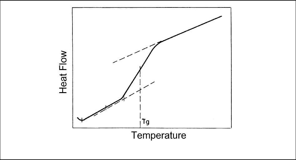
MIL-HDBK-17-1F

Volume 1, Chapter 6 Lamina, Laminate, and Special Form Characterization

6-30

which may be used to calculated T

. T

of neat resin specimens is relatively easy to detect with DSC, but

in composite specimens the resin content in the specimen is small, and the more highly crosslinked the

resin, the smaller the change in heat capacity. It is, therefore, sometimes difficult to detect

in highly

crosslinked cured composites (see Reference 6.6.3.2.1).

FIGURE 6.6.3.2.1 Differential scanning calorimetry (DSC).

6.6.3.2.2 Thermomechanical analysis (TMA)

Thermomechanical techniques such as expansion, flexure, or penetration thermomechanical analysis

(TMA) may also be used to determine

. In expansion TMA, the coefficient of thermal expansion

measured as a function of temperature. As noted above,

undergoes a change during the glass transi-

tion, and

is determined by the point of intersection of lines fit to the thermal expansion data above and

below the glass transition range. Figure 6.6.3.2.2 illustrates the specimen geometries and data reduction

methods used for various TMA techniques.

In flexural TMA, a rectangular specimen is loaded in bending and the dimensional change is meas-

ured as a function of temperature. A curve fitting technique as illustrated in Figure 6.6.3.2.2 is used to

calculate

. Flexural TMA measurement of T

is similar to heat distortion temperature (HDT) measure-

ment, since in both cases the specimens are loaded in flexure. An HDT specimen may be a full-size flex-

ural test specimen, and is loaded in three-point bending or as a cantilever beam. Displacement is meas-

ured as a function of temperature, and the HDT is the temperature at which the displacement reaches

some predetermined value. Use of a full-size specimen minimizes moisture loss during the HDT test, but

flexural TMA and HDT measurement share the disadvantage that values of

or HDT obtained will be

sensitive to the modulus of the reinforcing fibers in the composite sample and they will give different re-

sults depending on the nature of the fiber.

As shown in Figure 6.6.3.2.2, penetration mode TMA measures the hardness of the material. One

disadvantage of this technique is that if the probe is touching a reinforcing fiber, an accurate measure-

ment of the

of the matrix will not be obtained.

MIL-HDBK-17-1F

Volume 1, Chapter 6 Lamina, Laminate, and Special Form Characterization

6-31

FIGURE 6.6.3.2.2 Thermomechanical Analysis (TMA) - typical dimensions shown.

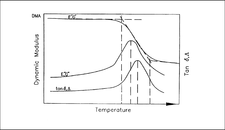
MIL-HDBK-17-1F

Volume 1, Chapter 6 Lamina, Laminate, and Special Form Characterization

6-32

6.6.3.2.3 Dynamic mechanical analysis (DMA)

Dynamic mechanical analysis (DMA) is the most common and preferred method of characterizing the

glass transition of organic matrix composites. There are several types of DMA which have been used

with composites, including torsion pendulum analysis (TPA) and other resonant techniques, and forced

oscillation measurements in tension, torsion, and shear. These forced measurements are made using a

number of DMA instruments, manufactured by DuPont, Perkin Elmer, Polymer Laboratory, Rheometrics,

TA Instruments, and others.

All these DMA techniques produce curves of dynamic storage and loss modulus and loss tangent (

tan

δ) or log decrement (Λ) as a function of temperature (see Figure 6.6.3.2.3(a)). Tan δ and Λ are propor-

tional to the ratio of the loss modulus (

E" or G") to the storage modulus (E' or G'). They reflect the amount

of energy dissipated during each cycle of loading, and go through a peak value during the glass transition.

may be determined from DMA data in several different ways, and this may be a source of differences in

reported values for

. As shown in Figure 6.6.3.2.3(a), T

may be determined as the temperature at the

onset or the midpoint of the transition based on the storage modulus curve, at the maximum in

tan δ, or at

the maximum in loss modulus. Clearly the method used for calculating

could produce markedly differ-

ent values for the same set of DMA data. The temperature scanning rate and frequency employed will

also affect the results, as discussed above.

FIGURE 6.6.3.2.3(a) Dynamic mechanical analysis (DMA).

An ASTM standard (D 4065) is available for DMA of plastics, covering both forced and resonant tech-

niques (Reference 6.6.3.2.3(a)). The test techniques described in this standard practice are the same as

those used for fiber reinforced plastics. In addition, a newly released SACMA method (SRM 18R-94) rec-

ommends the use of DMA for the measurement of

in oriented fiber-resin composites (Reference

6.6.3.2.3(b)). SACMA SRM 18R-94 specifies a forced oscillation measurement at 1 Hz, a heating rate of

5C° (9F°) per minute, and calculation of an onset

from the dynamic storage modulus curve. If a con-

sistent material operational limit (MOL) is to be calculated from

, standards for these experimental vari-

MIL-HDBK-17-1F

Volume 1, Chapter 6 Lamina, Laminate, and Special Form Characterization

6-33

ables should be specified along with a temperature safety margin. Otherwise the measured T

may be

shifted by increasing or decreasing heating rate or frequency.

As discussed above, measurement of

in a wet composite material is made more difficult by the

drying which occurs as the specimen is heated. Techniques which seek to prevent this drying by sealing

the specimen in some way may be helpful in slowing the weight loss, but it cannot be prevented com-

pletely. If the specimen is sufficiently thick, the drying will occur primarily at the outside surface, resulting

in a broadened or even bimodal glass transition (see Figure 6.6.3.2.3(b)). The lower temperature region

will reflect the

of the interior of the specimen which is still wet, and the higher temperature region will

reflect the

of the dried material. The loss tangent or log decrement curve will be broadened, or will ex-

hibit two peaks or a peak and a shoulder, with the relative peak heights indicating the amounts of wet and

dried material present in the specimen. In measuring

of a wet specimen, the lower temperature part of

the transition may be the region of interest, suggesting that calculation of an onset

would be the appro-

priate and conservative approach.

FIGURE 6.6.3.2.3(b) DMA of a wet composite material.

6.6.3.3 Glass transition test methods for MIL-HDBK-17 data submittal

Data generated by DMA as described above are currently being accepted by MIL-HDBK-17 for con-

sideration for inclusion in Volume 2. In addition to the specific apparatus used for the measurement, the

heating rate and frequency must be included, and the method used to calculate

from the data must be

specified. If a resonant method such as torsion pendulum is used, the frequency in the glassy region

should be included with the data.

6.6.3.4 Crystalline melt temperature

The crystalline melt temperature (

) of semi-crystalline thermoplastic composites can be obtained

from DSC or DTA experiments. In addition, an estimate of the degree of crystallinity can be made. This

becomes an important parameter since the properties of semi-crystalline thermoplastic composites may

be dependent upon the degree of crystallinity of the matrix resin. The heating required for processing

prepregs into composite structures may have an affect on the degree of crystallinity as well as the crystal

structure.

MIL-HDBK-17-1F

Volume 1, Chapter 6 Lamina, Laminate, and Special Form Characterization

6-34

6.6.4 Density

6.6.4.1 Overview

The density of composite materials is useful both directly, as for estimation of bulk weight or for ther-

mal or dynamic analysis, as well as indirectly, as in derivation of quantities based on other measure-

ments, like thermal conductivity (with specific heat and diffusivity) and void volume (with fiber and resin

density). The application will determine the optimum test method, each of which have different levels of

precision and bias (see Section 2.2.4) as well as different levels of ease of use. The last application men-

tioned, void volume determination of composites, probably has the most demanding density determina-

tion requirements. In order to accurately determine void volume to within 0.5% or better the density of the

composite and the constituents must be known to within about 0.005 g/cm

(1.8x10

-4

lb/in

) or better.

Density can be measured directly or calculated from separate volume and mass measurements.

From these two approaches the focus will be on the three main density test methods in current use, which

are: 1) Archimedes volume determination by liquid (most often water) displacement, as standardized by

ASTM D 792 (Reference 6.6.4.1(a)); 2) direct measurement of density by observation of the level at which

the test material is suspended in a density gradient column, as standardized by ASTM D 1505 (Reference

6.6.4.1(b)); and 3) measurement of test specimen volume by pressure changes of a known amount of an

inert ideal gas (helium pycnometry), as standardized by ASTM D 4892 (Reference 6.6.4.1(c)) for a non-

composite material and modified by MIL-HDBK-17 for use with composites as described in Section

6.6.4.4.1.

While all three test methods provide generally accurate density values, the helium pycnometry

method has not been demonstrated to be sufficiently accurate for use in determining void volume (see

evaluation results in Section 6.6.4.5), although this may change in time with future modifications to proce-

dure and instrumentation. For typical applications in composites, the Archimedes method, as described in

ASTM D 792 and modified below, is preferred for its low cost, relative simplicity, and high accuracy (when

properly performed). While also accurate, the density-gradient technique is less desirable due to the high

labor cost and low through-put (since it may take several hours for one determination to stabilize in the

column). Also, the long exposure of the specimen to the column fluid may not be desirable for subse-

quent procedures like matrix digestion. Each of the test methods is described in detail in the sections

below.

Liquids are used almost exclusively in displacement techniques. However, there are advantages to

using a gas medium in place of liquid to determine specimen volume. One advantage is minimization of

errors associated with liquid surface tension. The gas displacement approach is often referred to as he-

lium pycnometry. When helium pycnometry is used, the test specimen volume is determined by measur-

ing pressure changes of a confined amount of gas. Helium pycnometry is not yet a standardized test

method for measuring the volume and density of composites, yet it has been demonstrated to be a viable

technique (References 6.6.4.1(e) and (f)). As no test standard or guidelines exist for this method as ap-

plied to composites, a test procedure has been developed within the MIL-HDBK-17 Testing Working

Group. The procedure has been included as Section 6.6.4.4.1. This procedure will remain in effect until

such time as a standard method for composites is adopted by ASTM or another standard-certifying or-

ganization.

6.6.4.2 ASTM D 792, Standard Test Method for Density and Specific Gravity (Relative Density) of

Plastics by Displacement

Density of composites is frequently measured by means of ASTM D 792 which is under the jurisdic-

tion of ASTM Committee D-20 on Plastics. This standard actually describes a means of measuring

specimen volume and combines that value with a weight measurement to calculate density. Obtaining an

accurate volume measurement is the key to a reliable composite density value.

For a quick and convenient, but less accurate density determination method, the reader is referred to the micrometer technique as

specified in ASTM D2734, Test Method C (Reference 6.6.4.1(d)). This method obtains specimen volume by simple dimensional

measurement and is only appropriate for precision work in limited specific cases.

MIL-HDBK-17-1F

Volume 1, Chapter 6 Lamina, Laminate, and Special Form Characterization

6-35

The method is based on the weight of a specimen in air compared to its weight while completely im-

mersed in a liquid of known density, most often water. When using water as the medium it must be de-

gassed and either deionized or distilled for high accuracy work. A close eye must be kept for nucleated

gas bubbles which are most likely to appear on rough surfaces such as machined edges. Also, the ma-

chined surfaces are usually more porous and may not wet completely. Close scrutiny of these surfaces is

recommended to verify that no visible microbubbles are present within surface cavities. If microbubbles

are present, switch to a higher wetting liquid or add a surfactant (for example, add four drops of Cole-

Palmer 8790 Micro-Lab Cleaning Solution per 200 ml of water) for optimum results.

In general, the bigger the specimen the better. As specimen size and weight get closer to zero, the

measurement limits on volume and weight begin to affect the density value. The recommended minimum

test specimen is 1 gram (for carbon/epoxy this is about 0.037 in

(0.6 cm

), for glass/epoxy it is about

(0.024 in

0.4 cm

). A balance accuracy of 0.0001 g (2.2x10

-7

lb) is required for precision work on a

specimen of this size.

The D 792 test method states room temperature testing should be conducted after conditioning the

specimens for at least 40 hours at the standard laboratory atmosphere of 73.4 ±3.6°F (23 ±2°C) with 50

±5% relative humidity. If the test is being performed to referee a disagreement, the tolerances are ±1.8F

(±1C

°), and ±2% relative humidity. For cases where immersion liquids other than water are being used,

the temperature tolerance is ±0.9F

° (±0.5C°). For an improvement in precision, the ASTM D-30 commit-

tee recommends bringing the material to oven-dry equilibrium to determine the initial weight (References

6.6.4.2(a) and (b)).

Two techniques are offered: Test Method A, employing water as the immersion liquid; and Test

Method B using a liquid other than water, such as kerosene. Test Method B is often used when the

specimens are either lighter than water, or when water will cause the specimens to undergo physical

changes such as swelling.

Advantages and Limitations of ASTM Test Method D 792

The main advantages to choosing this method are practicality and precision (when carefully per-

formed), and it is by far the most frequently used method. Equipment needed is simple and inexpensive,

with the exception of a quality analytical balance. With careful technique, accuracy within ±0.005 g/cm

(±1.8x10

-4

lb/in

) is typically obtained. The apparatus includes a balance, a bridge for spanning the bal-

ance pan, a wire or filament, beaker, tweezers, thermometer, water or other liquid, and perhaps some

sinking weights if the specimen is less dense than the liquid.

After a time investment of about a day for practicing the technique so that reproducible results can be

obtained, the tests can begin. Four to six specimens per hour can typically be tested using D 792, how-

ever, there is a certain amount of tedium associated with this technique and actual through-put will likely

be lower.

As with all the density methods mentioned here, it is good practice to take care in specimen prepara-

tion, especially edge quality. Care must be exercised in cutting specimens to avoid density changes.

Other issues to be mindful of are specimen size, surface wetting (some experimenters add trace amounts

of surfactants to the water), liquid absorption during measurement, and water temperature (vacuum de-

gassing will cool the water, slightly changing its density). D 792 relies on a liquid medium, and problems

with entrapped and/or clinging gas bubbles are a concern. High wetting, degassed liquids are required

for optimum results.

6.6.4.3 ASTM D 1505, Standard Test Method for Density of Plastics by the Density-Gradient Technique

ASTM D 1505 is significantly different from D 792 in that specimen density is measured directly; no

calculations are used. It determines density by floating the test specimen in a glass column containing a

liquid mixture of known varied density. Composite specimens work well with this technique as long as the

liquid medium selected is inert to the specimens. The test is useful for tracking materials that undergo

MIL-HDBK-17-1F

Volume 1, Chapter 6 Lamina, Laminate, and Special Form Characterization

6-36

physical changes over time, checking uniformity, and identifying materials. It has also been reported to

be more precise, and likely, more accurate than the D 792 method (Reference 6.6.4.3).

The method uses two approaches: an incremental varied-density liquid column (Test Method A), and

two continuous varied-density liquid columns, Test Method B, progressively less dense liquid, and Test

Method C, progressively more dense liquid. When the column is filled correctly the gradient remains re-

markably stable and linear. The densities of the starting liquids are first closely approximated using a

calibrated volumetric canister (liquid pycnometer). Calibrated sink floats are used to determine the linear

variation of liquid density with the height of the column. By noting the level at which the specimen floats,

the density of the specimen can be matched to the known density of the column liquid at that height. The

accuracy and precision of this test are set by the sink floats along with a highly linear density variation of

the column liquid vs. height.

Advantages and Limitations of the ASTM Test Method D 1505

Equipment for this method can be purchased commercially for a few thousand dollars. This includes

an assortment of column fluids and sink floats. Alternatively, the apparatus can be assembled from stan-

dard lab glassware and components for minimal cost, but expect to spend time on machining and assem-

bly before any testing can be done.

The procedure for filling the column to make a linear gradient is best described as “artful.” Expect to

invest several days to a week learning this portion of the procedure. The column sensitivity is under the

control of the experimenter. A skilled experimenter can make columns that are in the range of

0.001g/cm

/cm (9.2x10

-5

lb/in

/in). Column sensitivity can be adjusted up or down to match the test need.

Sensitivity is set by the density difference of the starting liquids.

Once the column is ready, specimens should be carefully introduced at the top with tweezers. To

avoid gas bubbles clinging to the specimen it is helpful to set aside a small amount of the liquid mixture to

pre-wet the specimens. As with D 792, if bubbles are present they can often be seen through the glass

and transparent liquid, although there is not much that can be done to rectify this in the case of D 1505:

once a specimen is immersed it is extremely difficult to retrieve without destroying the gradient.

The D 1505 test itself is rather time-consuming. The column must be filled slowly and carefully to

preserve the gradient and typically takes several hours. Once the specimens are immersed it takes time

for them to settle to their equilibrated height in the column. If many specimens need to be measured, one

column will not be able to handle them all, so several gradient columns will have to be set up, broken

down, and refilled.

As with all the density methods mentioned here, care must be exercised in cutting specimens to avoid

density changes. The concerns with using a liquid medium are the same as those mentioned for D 792 in

the last paragraph of the above Section 6.6.4.2.

6.6.4.4 Use of helium pycnometry to determine density of composites

Technological advances in electronics and automation have made it possible to obtain accurate and

reliable volume determinations of composites (as well as fibers and matrix resins) using a gas in place of

liquids. Helium pycnometry is a method for measuring the volume of solids of all types, including powders

and open and closed cell materials. This flexibility is made possible because the medium used is an inert

ideal gas, usually helium, which will penetrate the tiniest pores. High purity helium is the most commonly

recommended gas because it is completely inert. High purity nitrogen is a good alternative to helium.

Helium pycnometry is not a new technology. Pycnometers, using both liquids and gases, have been

used in ASTM test standards for many years. However, it was not until fairly recently that helium pyc-

nometers became sophisticated enough to be used for high accuracy volume determinations. ASTM

adopted standard D 4892 (Reference 6.6.4.4) in 1989, which uses a helium pycnometer to determine the

volume/density of a non-composite material to three decimal places.

MIL-HDBK-17-1F

Volume 1, Chapter 6 Lamina, Laminate, and Special Form Characterization

6-37

Interest in using helium pycnometry to measure composite density stems from its potential to be both

as accurate and precise as D 1505 while at the same time having a higher through-put and better ease of

use than D 792. Another distinct advantage of using a gas medium is that it guarantees reproducible

penetration into surface pores. With a liquid medium the experimenter has no way of knowing what per-

centage of the surface porosity is left unfilled.

In helium pycnometry the volume of solid objects is measured by employing Boyle's Law, which

states that the decrease in volume of a confined gas results in a proportionate increase in pressure. Both

helium and diatomic nitrogen are used because they behave as ideal gases at room temperature. A he-

lium pycnometer makes use of this by making two precise pressure measurements on two known cali-

brated volumes. These are the cell volume and the cell volume plus a smaller expansion volume usually

called the "added volume." The first pressure is measured with all gas confined in the main measurement

cell where the test material is located. After this pressure is determined a valve is opened connecting the

main and expansion cells together. This results in a second, lower pressure which is recorded. Using the

ideal gas law the volume of the test material in the main cell is determined using the equation below in

Section 6.6.4.4.1.

Advantages and Limitations of the Helium Pycnometry Procedure

A distinct advantage of using a gas medium is that it guarantees reproducible penetration into surface

pores. With a liquid medium the experimenter has no way of knowing what percentage of the surface

porosity is left unfilled.

The accuracy of this method begins to drop off when the ratio of the sample volume to test cell vol-

ume (

) is low. Experiments have shown that if this ratio is approximately 30% or higher the pyc-

nometer will be near its optimal performance (References 6.6.4.1(e) and (f)). This is not to say that useful

data can not be obtained when the ratio is below 30%. The precision and bias remain quite useful to low

ratios below 1% (References 6.6.4.1(e) and (f)). The ratio needed for a particular test is determined by

the accuracy needed; for example, if one significant digit is sought, then there would be no restriction on

the

ratio. However, if three digits are needed the V

ratio becomes important and should be 0.3

or higher.

The gas pressure is sensitive to temperature. Tests were run to detect temperature fluctuation in the

measurement cell. It was found that no matter what cell volume was used, the internal temperature of the

measurement cell was extremely stable, despite the constant influx and expansion of fresh helium (Ref-

erence 6.6.4.1(f)).

The shape of the test specimen can cause problems during insertion into the measurement cell. The

cells of off-the-shelf pycnometers sold today are usually cylindrical. If the test specimen is restricted to

some rectangular shape it may be difficult to get more than 30% of the cell volume filled due to geometric

incompatibility. Commercially available pycnometers are like this because, although capable of working

with any solid object, they are designed for their most popular application, which is powders. This prob-

lem can be remedied by cutting the composite specimen to match the cell geometry, for example, stacked

disk-shaped specimens.

A quality helium pycnometer, such as the one used in this work, is a sophisticated piece of analytical

equipment with a base cost in the $10,000 range. Much like a lab analytical balance, once the equipment

is purchased very modest costs are associated with the test thereafter. Expect to spend several days

getting familiar with the equipment and procedures.

Pycnometry has an advantage in that much less labor is involved, as the equipment is automated.

Aside from sample preparation and conditioning, the experimenter needs to change specimens at the end

of each run. Once running, the pycnometer gathers data at a rate of 25 to 30 measurements per hour.

An important aspect of automation is that it significantly reduces variations introduced by operator-to-

operator skill and "artfulness" which enter into the test results.

MIL-HDBK-17-1F

Volume 1, Chapter 6 Lamina, Laminate, and Special Form Characterization

6-38

As with all the density methods mentioned here, care must be exercised in cutting specimens to avoid

density changes.

6.6.4.4.1 Helium pycnometry test procedure for determining composite density

Helium pycnometry is not a formally recognized method for measuring composite density. As no test

standard or guidelines exist for this method, a procedural guideline is included here. This procedure will

remain in effect until such time as a standard test method is adopted.

Background

Volume and density of solid objects is measured by employing Boyle's Law, which states that the de-

crease in volume of a confined gas results in a proportionate increase in pressure. Both helium and dia-

tomic nitrogen behave as ideal gases at room temperature. As noted above, the pycnometer makes use

of this by making two precise pressure measurements on two known volumes. These are the cell volume

and the cell volume plus a smaller expansion volume usually called the "added volume." The working

equation used to calculate the test specimen volume is

−

(/)

6.6.4.4.1

where

= specimen volume

= previously calibrated empty specimen cell volume

= previously calibrated added volume

= pressure when all gas is confined to the main cell

= second pressure when the gas fills both cells

Before running the pycnometer,

and V

are calibrated by using a volume calibration standard. As-

sumptions made are that the cell temperature is constant, the two cell volumes are constant, and the

moles of gas present is constant. The specimen density is obtained by supplying the pycnometer with a

weight measurement of the test material from an analytical balance.

Testing has shown that when the

ratio is approximately 30% or higher the pycnometer will oper-

ate near optimal performance. This is not to say that reliable data can not be obtained when the ratio is

below 30%, but rather, some loss in performance begins to occur.

It is important to note that the gas medium guarantees filling the tiniest of surface pores, which other

liquid immersion methods may or may not do, due to surface tension. This should be kept in mind when

comparisons are made. When surface pores are not filled the density data is shifted to some lower value.

Therefore, liquid immersion methods may return density data that is biased slightly to the low side when

compared to data from the helium pycnometry method. This density shift may or may not be noticeable,

depending on such factors as the amount of surface porosity and the wetout between the liquid and the

composite.

Apparatus

Helium pycnometer (the pycnometers specified in ASTM D 4892, Footnote 4 are acceptable for use

here); volume calibration standard; high purity helium or nitrogen gas cylinder with regulator; analytical

balance; desiccator; disposable plastic gloves or tweezers (for specimen handling).

Specimen Preparation

Heat and pressure from the specimen cutting process can locally alter the specimen density. Com-

posite specimens should be sanded with fine grit paper and wiped clean of any remaining loose dust.

Specimen shape is irrelevant to the test, but consideration of specimen geometry is required in order to

ensure enough material gets into the measurement cell. The recommended shape for a cylindrical cell is

MIL-HDBK-17-1F

Volume 1, Chapter 6 Lamina, Laminate, and Special Form Characterization

6-39

a circular specimen with a diameter nominally 0.080 inches (2.0 mm) less than the cell diameter. Speci-

men diameter can be larger, but not so large that there is a risk of jamming against the cell walls. The

disks should be stacked to fill as much of the cell as possible. If significantly lower precision is accept-

able, there is no need to consider what percentage of the cell volume is filled (unless the specimen vol-

ume is extremely small). Useful data will result even when

is near 1% (References 6.6.4.1(e) and

(f)).

Procedure

1. Precondition the test specimens according to ASTM D 618 "Conditioning Plastics and Electrical

Insulating Materials for Testing" (Reference 6.6.4.4.1(a)) or, for improved accuracy, bring the

specimen to oven-dry equilibrium as recommended by References 6.6.4.2(a) and described by

6.6.4.2(b). Store the test specimens in a desiccator at 73.4°F (23°C) until they are ready to test.

2. In general, follow the manufacturer's instructions to determine the composite density. A list of,

and comments on, the test steps is given here.

• The helium (or nitrogen) source should be connected to the pycnometer gas input via a gas-tight

pressure fitting.

• The printer and computer (if so equipped) should be connected to the data output interface via an

appropriate cable.

• After the pycnometer power is turned on, let it warm up to its equilibrium operating temperature,

which is typically 3.6 to 5.4F

° (2 to 3C°) above ambient temperature.

• If the pycnometer has not been calibrated, run the calibration procedure specified in the user’s

manual. From time to time the pycnometer should be recalibrated, especially if the ambient tem-

perature has changed by an appreciable amount or if it fluctuates. The pycnometer is only as

good as the calibration standards used to calibrate it. Be sure the standards used meet proper

specification. If the accuracy of the standards is in doubt they can be spot-checked using a test

such as D 792. Certified standards can be obtained through the National Institute of Standards

and Technology (Reference 6.6.4.4.1(b)).

• Once calibrated, the pycnometer is ready to run. Remove the sealed cap, opening the main cell

to the ambient air. Place the pre-weighed test specimen inside the cell. The cap is then replaced

and the run started. Before measurement begins the pycnometer typically purges itself for sev-

eral minutes with helium. This serves two purposes; it ensures that only helium is in the cell and

it carries off residual moisture from the specimen surface. At this point the actual measurement

runs begin.

• If the pycnometer is automated it will rerun the same specimen a pre-selected number of times

and, when completed, will print a summary of the run, including the average volume and density

with their associated standard deviations. Automated machines will download the raw data and

the report to a personal computer if desired. Once the download is complete the pycnometer is

ready to repeat the measurement cycle.

• Change out the specimens, re-seal the measurement cell and begin a new run. Recalibration is

not necessary for continuous use if the ambient temperature is stable.

6.6.4.5 Summary of helium pycnometry experimental results

A high quality helium pycnometer (Quantachrome Ultrapycnometer 1000) was tested to determine its

viability as a tool for measuring the volume/density of composites. Conclusions reached as a result of

this testing are as follows (refer to References 6.6.4.1(e) and (f) for all conclusions):

MIL-HDBK-17-1F

Volume 1, Chapter 6 Lamina, Laminate, and Special Form Characterization

6-40

• The D 792 method was more accurate with a maximum deviation of 0.003 g/cm

(1.1x10

-4

lb/in

)

from the certified value for the specimen volumes used. More typically the data varied within

0.001 g/cm

(3.6x10

-5

lb/in

) of the NIST standard.

• Above 30% fill of the measurement cell the pycnometer data deviated by a maximum of 0.003

g/cm

(1.1x10

-4

lb/in

). More typically the data varied within 0.002 g/cm

(7.2x10

-5

lb/in

) of the

standard. Below 30% fill the maximum deviation was 0.015 g/cm

(5.4x10

-4

lb/in

) and a fall off in

accuracy with decreasing

was evident.

• The standard deviations of the two techniques are comparable and tight with the pycnometer data

showing slightly tighter or equal values for all data points. The typical standard deviation for the

D 792 method was 0.001 g/cm

(3.6x10

-5

lb/in

) while the standard deviations for the helium

pycnometer typically ranged from 0.0008 to 0.0002 g/cm

(2.9x10

-6

to 7x10

-7

lb/in

). The maxi-

mum standard deviation recorded by the pycnometer was 0.003 g/cm

(1.1x10

-4

lb/in

). The larg-

est standard deviation of the D 792 method was 0.004 g/cm

(1.4x10

-4

lb/in

) recorded in two in-

stances.

• The pycnometer data have a persistent tendency to read slightly below the actual density value

as if a constant offset phenomena was occurring. The reason for the low offset is not known at

this time.

One difference between gas and liquid mediums is that gases are much more susceptible to tempera-

ture variations. The periodic influx of cool helium, and the further cooling of the helium due to expansion

was initially a concern as this situation could cause erroneous low pressures to be recorded. Testing

showed that the thermal environment in the sample cell is extremely stable, with the helium temperature

worst case recovery time of 9 sec. The worst case maximum deviation value reached was -3.8F

(-2.1C

°), which occurred within 50 milliseconds after expansion. From this data it is concluded that the

gas expansion is not an issue and that the helium is quickly reheated by the thermal mass of the sample

cell. Further, 200 repetitions of the gas expansion event showed no change in the temperature recovery

curve or any drop in the cell temperature over time, indicating that the sample cell has ample heat capac-

ity to maintain a stable temperature environment for an indefinite period.

6.6.4.6 Density test methods for MIL-HDBK-17 data submittal

Data produced by the following test methods (Table 6.6.4.6) are currently being accepted by MIL-

HDBK-17 for consideration for inclusion in Volume 2.

TABLE 6.6.4.6 Composite density test methods for MIL-HDBK-17 data submittal.

Property Symbol Fully Approved, Interim, and Screening Data Screening Data Only

Density

D 792, D 1505, 6.4.4.4.1* D 2734C

*When this method is used to generate data for subsequent determination of composite void volume,

the test specimen must occupy at least 30% of the test cell volume.

6.6.5 Cured ply thickness

NOTE: Throughout this discussion the term "cured" refers to a fully processed state. For thermosetting

materials it means chemically cured. For thermoplastic materials it denotes a fully consolidated condition.

MIL-HDBK-17-1F

Volume 1, Chapter 6 Lamina, Laminate, and Special Form Characterization

6-41

6.6.5.1 Overview

The thickness of a composite part is an important property from the standpoint of weight and dimen-

sional compliance (fit) in hardware applications. Part thickness is governed by the number of plies in the

lay-up, the amount of matrix resin present (resin content), the amount of reinforcing fiber (fiber volume),

and the amount of porosity (void volume). In the case of resin transfer molding (RTM), the tool dimen-

sions dictate thickness (by controlling resin content). If it is assumed that the amounts of resin, fiber, and

porosity do not vary from one ply to another within the structure, then the thickness per ply times the

number of plies is representative of the part thickness. In practice, the proportions of resin, fiber, and po-

rosity may vary somewhat from ply to ply. The magnitude of this variation is largely a function of process-

ing parameters. For example, surface bleeding during cure may produce lower resin content in the outer

plies compared to interior plies, depending on the mobility of the resin through the part thickness. How-

ever, the average cured ply thickness multiplied by the number of plies generally provides a reasonable

estimate of part thickness.

Since test panel laminates are typically processed in a manner that simulates a production part proc-

ess, panel cured ply thickness may also be used to estimate part thicknesses. In addition, cured ply

thickness of a test panel may be used in the calculation of fiber volume and subsequent normalization of

mechanical test data (see Section 2.4.2 on normalization).

Determination of cured ply thickness generally involves measuring the thickness of a laminate (panel

or part) in a number of locations, averaging these thickness values, and dividing by the number of plies in

the lay-up. Laminate thickness can be measured by direct means (using devices such as micrometers) or

indirectly (using ultrasonic instruments). Sections 6.6.5.2 and 6.6.5.3 below briefly discuss the use of di-

rect and indirect means of measuring laminate thickness. Section 6.6.5.4 discusses SRM 10R-94, which

is the only current standard for measuring cured ply thickness.

6.6.5.2 Thickness measurement using direct means

Deep throat micrometers are typically used to directly measure thickness at various locations over the

laminate surface. While this is a fairly straight forward procedure, there are several issues to consider.

First is the matter of panel or part size and shape. If the laminate to be measured has large length

and width dimensions, the micrometer may not reach far enough into the interior. This problem may be

overcome by substituting a dial indicator or similar device suspended from a rigid framework, but accu-

racy is usually sacrificed. Also, if the laminate has curvature, the micrometer throat may interfere to the

extent that the anvils will not reach the laminate surfaces. Laminate surface texture is another significant

issue. The reader is referred to Section 6.4.2 for a detailed discussion of this topic. If the size and shape

of the laminate do not present a problem, ball-faced micrometers offer an accurate, low cost means of

direct thickness measurement.

6.6.5.3 Thickness measurement using indirect means

Pulse-echo type ultrasonic equipment can be used to measure laminate thickness. This technique

makes use of the fact that sound can be directed through a laminate, reflected from the opposite surface,

and its traverse time measured. If the sound velocity through the laminate material is established by test-

ing specimens of known thickness, then the unknown laminate thickness can be calculated. ASTM E797-

90 (Reference 6.6.5.3(a)) describes this practice, but does not include detailed information or any specif-

ics relative to measurement of composite laminates.

One advantage of using an ultrasonic method is that access to only one surface is required. This is

important for measuring skin thickness on closed structures, or for measuring large laminates where mi-

crometer measurement is not possible. However, the disadvantages are considerable. First, the equip-

ment can be expensive relative to other options. Second, calibrations must be run on specimens of

known thickness. This must be done for each specific material to be tested since sound velocity may be

different for each. A further complication is that velocity is also affected by the ratio of fiber to matrix resin

MIL-HDBK-17-1F

Volume 1, Chapter 6 Lamina, Laminate, and Special Form Characterization

6-42

in the laminate and, in fact, SACMA method SRM 24R-94 (Reference 6.6.5.3(b)) takes advantage of this

very fact to estimate resin content of prepreg. Third, surface texture is a concern as discussed earlier in

Section 6.6.5.2.

Because of the significant disadvantages, this measurement method is not recommended where di-

rect measurement using a micrometer or similar device is possible.

6.6.5.4 SRM 10R-94, SACMA Recommended Method for Fiber Volume, Percent Resin Volume and Cal-

culated Average Cured Ply Thickness of Plied Laminates

The cured ply thickness portion of this method (Reference 6.6.5.4) specifies that thickness readings

be taken in at least 10 locations over the surface of the laminate using a ball-faced micrometer. It is rec-

ommended that no readings be taken closer than one inch (25 mm) from any edge. The average lami-

nate thickness is calculated and divided by the number of plies to obtain an average cured ply thickness.

The method recommends that a laminate be subdivided for the calculation of fiber volume if the variation

in laminate thickness exceeds 0.008 inch (0.2 mm). This indirectly suggests that a single cured ply thick-

ness should not be calculated under such conditions.

6.6.5.5 Cured ply thickness test methods for MIL-HDBK-17 data submittal

Methods which meet the requirements of SRM 10R-94 are acceptable when submitting data to MIL-

HDBK-17 for consideration for inclusion in Volume 2. In addition, cured ply thickness may be calculated

using measured thicknesses of test specimens obtained from a panel provided there are at least 10

specimens distributed over the entire area of the panel (so as to be equivalent to SRM 10R-94).

6.6.6 Fiber volume (V

) fraction

6.6.6.1 Introduction

The fiber volume (expressed as a fraction or percent) of cured polymer-matrix composites is com-

monly obtained by matrix digestion, ignition loss, areal weight, and image analysis methods. These meth-

ods generally apply to laminates fabricated from most material forms and processes, but the areal weight

method cannot be used for filament wound material or other forms that do not consist of discrete individ-

ual plies. Each method has its benefits and drawbacks. Other less common methods will not be dis-

cussed.

6.6.6.2 Matrix digestion

The method of matrix digestion is covered under ASTM Test Method D 3171 “Fiber Content of Resin-

Matrix Composites by Matrix Digestion” (Reference 6.6.6.2). The technique is based on digestion of the

matrix by a suitable liquid which does not attack the reinforcing fibers. Depending on the resin, three dif-

ferent procedures are used: Procedure A, concentrated nitric acid; Procedure B, aqueous mixture of sul-

furic acid and hydrogen peroxide; and Procedure C, a mixture of ethylene glycol and potassium hydrox-

ide. For example, epoxies generally respond well to all three procedures. Although toughened systems

respond better to procedure B, some fiber types are attacked more by B than by A. BMI’

s, polyimides, and

thermoplastics usually respond well to procedure B. Aramid fibers are attacked by both A and B, and

therefore, procedure C works best on aramid fiber composites.

Possible causes of error:

If the fiber is significantly attacked by the digestion fluid, results will be erroneous. It is recommended

to validate the process by testing a control sample of only fiber to determine mass change of fiber

during test.

Some toughened resin systems have additives such as elastomers or thermoplastics. If these addi-

tives are not dissolved by the digestion fluid, they may cling to the fiber causing erroneous results.

MIL-HDBK-17-1F

Volume 1, Chapter 6 Lamina, Laminate, and Special Form Characterization

6-43

Incomplete digestion of the resin.

Sample size must be large enough to be representative and weighed accurately.

Accuracy is dependent on accuracy of density measurements.

6.6.6.3 Ignition loss

The method of ignition loss is described in standard test method ASTM D 2584 “Ignition Loss of

Cured Reinforced Resins.” The technique determines ignition loss of cured polymer-matrix composites

which can be considered to be the resin mass. A weighed specimen is heated until the resin matrix is oxi-

dized and converted to volatile materials. After removing any remaining ash, the residue (reinforcing fiber)

is weighed and the percent loss is calculated. Fiber density and composite density (to three significant

figures) are required in order to calculate fiber volume.

Possible causes of error:

If the fiber gains or loses weight under the conditions of the test, the results will be erroneous. (For

this reason, this procedure is not appropriate for aramid fibers and requires special temperature controls

for carbon fibers.)

Fillers, if present, must be oxidized with resin.

Incomplete decomposition of resin (and fillers, if present) during the test.

Any volatiles such as water, residual solvent, etc., will cause error unless they are small enough to be

ignored.

If the sample is heated too rapidly, mechanical loss of noncombustible residue (fiber) can occur, caus-

ing erroneous results.

6.6.6.4 Areal weight/thickness

Sections 6.6.6.2 and 6.6.6.3 discussed methods for determining fiber volume by destructively sepa-

rating the fibers from the matrix through chemical or thermal means and measuring the mass of the fibers

in a sample. As discussed in Section 2.4.3 on data normalization, there is a relationship between lami-

nate (or specimen) thickness and fiber volume for given values of fiber areal weight and fiber density.

This fact provides the basis for another method of fiber volume determination, which is not destructive.

In general the method involves measuring the laminate or specimen thickness and calculating the

fiber volume using this measured thickness, the number of plies in the laminate, and previously deter-

mined values of fiber areal weight and fiber density. Equation 6.6.6.4(a) or an equivalent form is used.

FAW n

=×

6.6.6.4(a)

where

= fiber volume fraction

FAW = fiber areal weight (mass per area per ply)

n = number of plies in the laminate

t = measured laminate (or specimen) thickness

= density of the reinforcing fiber

k = units conversion factor (if required)

MIL-HDBK-17-1F

Volume 1, Chapter 6 Lamina, Laminate, and Special Form Characterization

6-44

The calculated fiber volume is the reinforcing fiber’s contribution to the total volume. Although void

content does affect the laminate thickness (and hence fiber volume), it is not a factor in the calculation

since it contributes to total volume in the same way as the resin or any other non-reinforcement compo-

nent. Since the calculation requires the number of plies, the method is applicable only to material forms

with distinct plies for which fiber areal weight can be determined.

This general procedure is documented in SRM 10R-94 (Reference 6.6.6.4(a)), which references other

SACMA Recommended Methods for determination of fiber areal weight and fiber density. The specimen

defined by this method is a laminate panel, but the concept could be extended to individual test speci-

mens or to application parts. The method notes that the fiber areal weight and fiber density used in the

fiber volume calculation must be representative of the sample (panel, specimen, or part) under evaluation.

This is an important point. Although resin content may typically be the major factor affecting fiber volume,

fiber areal weight and fiber density variations can also have a significant effect on the accuracy of this

method. “Typical” or “data sheet” values for these parameters should not be used in the calculation.

SRM 10R-94 recommends that, as a minimum, fiber areal weight of the individual prepreg roll and lot av-

erage fiber density be used. If careful thickness measurements are taken (see Section 6.6.5) and appro-

priate fiber areal weight and fiber density values are used, this method can be quite accurate, and poten-

tially more reliable than destructive methods that depend heavily on laboratory technique.

For certain types of specimens the accuracy of thickness measurements may not be sufficient to yield

accurate fiber volumes. In particular, very thin specimens present the problem of obtaining three signifi-

cant figure precision. In addition, thickness cannot be reliably measured for specimens with irregular sur-

faces. As an alternate to measuring specimen thickness directly, it may be calculated using equation

6.6.6.4(b):

6.6.6.4(b)

where

= calculated laminate (or specimen) average thickness

M = mass of the specimen

A = surface area of the specimen

= measured density of the composite specimen

Combining equations 6.6.6.4(a) and 6.6.6.4(b) yields the following expression for fiber volume fraction in

terms of laminate specimen mass, density, and area:

FAW A n

×× ×

=×

6.6.6.4(c)

When mass is in grams, FAW in g/m

, densities in g/cm

, and area in in.

, then k = 1/1550.

For this variation of the method, the specimen must be extracted from the laminate or part such that

its edges are cut cleanly without any fraying. Ideally the specimen should be rectangular to permit area

calculation from specimen length and width. If possible, the specimen should be cut at least one inch

from any laminate (part) edge to minimize edge effects caused by fiber wash. The specimen mass is ob-

tained by weighing on a balance with adequate precision, and density is measured using archemedian or

other suitable methods (see Section 6.6.4 of this volume). More detail may be found in Reference

6.6.6.4(b).

Possible causes of error:

MIL-HDBK-17-1F

Volume 1, Chapter 6 Lamina, Laminate, and Special Form Characterization

6-45

• Inaccuracies in measured thickness caused by use of inappropriate measuring equipment, particu-

larly on textured surfaces (see Section 6.4.2).

• Inaccuracies in calculated surface area (for the area variation of this method) caused by edge dam-

age induced during specimen cutting or by inappropriate measuring equipment or technique, espe-

cially for irregularly shaped specimens.

• Wide variation in measured thickness across the specimen (in which case the calculated average

fiber volume is not representative of all areas of the specimen).

• Significant fiber wash (spreading) during cure (which causes an effective reduction in fiber areal

weight in the specimen compared to the value measured for the prepreg).

• Use of fiber areal weight and/or fiber density values that are not representative of the fiber in the

specimen.

6.6.6.5 Determination of fiber volume using image analysis

6.6.6.5.1 Background

The method of image analysis offers a technique of measuring fiber volume that eliminates the crea-

tion of waste chemicals while providing information about void volume laminate orientation and through

thickness fiber distribution. The basic assumption for this technique is that the evaluation of the two di-

mensional distribution of fibers through a random cross section is representative of the volumetric fiber

distribution. This assumption is valid for fibers of constant cross section, such as is found in tape lami-

nates, but is not valid for woven laminates. This technique works well for carbon fibers in a polymer ma-

trix, and for other fiber/matrix combinations where adequate contrast can be achieved. It does not, for

example, work as well for glass fibers, since the low contrast between the glass fibers and surrounding

matrix makes accurate measurements very difficult. There are no industry standard test methods for this

type of evaluation. Therefore, this section will describe the procedure in general terms. Computer soft-

ware for image analysis is commercially available.

6.6.6.5.2 Apparatus

This technique requires the use of metallographic specimen preparation equipment, a reflected light

microscope with a magnification of at least 400 times which has the capability of porting the image to a

digital camera, a computer with image acquisition card and image analysis software. While automated

image acquisition systems are available, this analysis can also be performed by manual specimen trans-

lation and focusing. The use of software macros can reduce the time required to process a fiber volume

measurement. Macros allow the user to automate repetitive software instructions.

6.6.6.5.3 Specimen preparation

A small section of laminate is prepared using standard metallographic techniques. A typical specimen

is ¾ inch (2 centimeters) on a side. The cross section is taken across the thickness of the laminate. The

orientation of the cross section with respect to the laminate is dependent on the orientation of the fibers in

the laminate being evaluated. The image analysis technique can be used to evaluate fiber volume in

laminates with ply orientations from 0 to approximately 60

°. At angles above 60 degrees the fiber edge

definition becomes distorted by the subsurface fibers. If a laminate with 0/90 lay-up is evaluated, the

laminate can be sectioned at 45

° to enable evaluation of the fiber volume in all plies. If fiber volume is to

be measured on a 0/

±60 laminate, the cross section can be oriented at 0° so that all plies can be evalu-

ated.

The surface of the polished specimen should display a clear delineation between the fibers and the

matrix. The fiber volume measurement should be made at as high a magnification as possible. This to

MIL-HDBK-17-1F

Volume 1, Chapter 6 Lamina, Laminate, and Special Form Characterization

6-46

some extent depends on the fibers being examined, but for most fibers a magnification of at least 400 to

1000 times should be used. This should get 30 to 100 fibers in the field of view. As these are areal

measurements being performed, the partial fibers can be included in the analysis. This would not be true

if the individual fiber area were being determined. A typical image is shown in Figure 6.6.6.5.3.

FIGURE 6.6.6.5.3 Typical grayscale image (M55J fibers).

6.6.6.5.4 Image analysis

The objective of the fiber volume image analysis technique is to discriminate between the fibers and

matrix. The image is acquired as a gray scale, threshold intensity is used to select the delineation point

between the fibers and matrix. The threshold level can be determined by evaluating a histogram of the

image as shown in Figure 6.6.6.5.4(a). Typically once the threshold is selected for a given cross section it

does not have to be altered as additional images are acquired for that specimen. It is good practice to

display the histogram while acquiring images to confirm the veracity of the threshold level. The threshold

level is used to convert the grayscale image to a binary image (Figure 6.6.6.5.4(b)) where the fibers will

be either black or white and the matrix will be the opposite (white or black). The computer then counts

the number of black and white pixels, and the ratio of the fiber pixels to the total number of pixels in the

image is the fiber volume.

While automated image systems can be programmed to analyze the entire cross section, this may

require as many as 1000 images. Accurate results can be obtained from manually operated systems us-

ing from 20 to 50 samples. Testing has shown that where the fibers/resin are evenly distributed, the

mean fiber volume converges to a constant value in as few as 20 samples. The manual sampling should

be distributed throughout the cross section.

The typical steps in the analysis of a single frame are:

1. Position the specimen. (Manually/automatically move the stage on which the specimen rests.)

2. Focus the microscope. (Manual focusing requires the use of a real time monitor on older computers.

Newer computers have acquisition rates fast enough to preclude the use of a monitor.)

3. Acquire an image. (The image used to measure the fiber volume may be a single frame or an aver-

age of multiple frames. Integrating several images can offset low luminescence of an image. Exami-

nation of the histogram will indicate if the image is suitable for evaluation.)

4. Identify pixels corresponding to fibers. (The histogram should be checked to insure that the correct

threshold value has been selected.)

5. Create a binary image. (The pixels with values greater than the threshold value will be black and the

pixels with values less than the threshold value will be white.)

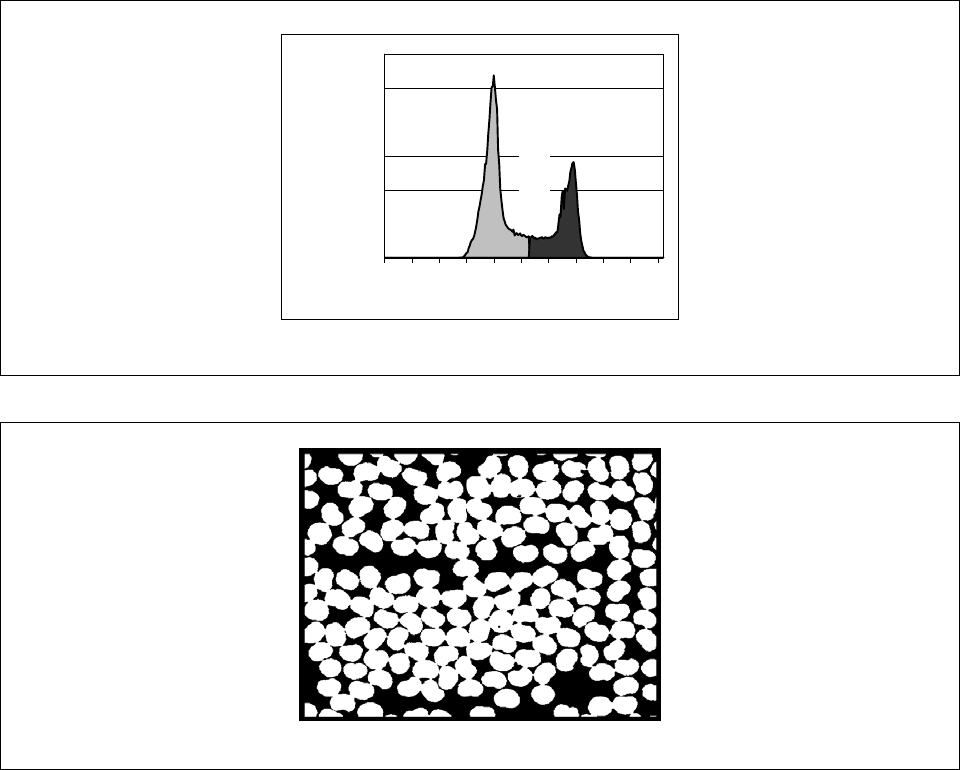
MIL-HDBK-17-1F

Volume 1, Chapter 6 Lamina, Laminate, and Special Form Characterization

6-47

6. Count the number of white and black pixels. (Typically it will be necessary to obtain a count of only

one of the colors. The total number of pixels in the frame remains constant so the number of fiber

pixels for a given image is all that needs to be recorded.)

Histogram

2000

4000

6000

8000

10000

12000

Intensity (0-255)

Pixel Counts

Fibers

Matrix

Threshold

FIGURE 6.6.6.5.4(a) Typical histogram of gray scale fiber and matrix distributuion.

FIGURE 6.6.6.5.4(b) Binary fiber image.

The time required to process a fiber volume measurement can be accelerated by the use of macros

within the image analysis program. After the microscope has been focused (step 2), a macro can be initi-

ated via a single keystroke which initiates the acquisition sequence (steps 3 through 6). The histogram

can be displayed so that the operator can verify the adequacy of the threshold value selected. Some im-

aging software programs will have an automatic threshold operation.

6.6.6.5.5 Sources of error

• Out of focus or dirty optics can distort the image which in turn will give inaccurate results.

• Poor metallographic preparation techniques of the cross-section surface makes accurate thresholding

difficult.

• Insufficient magnification will result in poor definition of the fibers.

MIL-HDBK-17-1F

Volume 1, Chapter 6 Lamina, Laminate, and Special Form Characterization

6-48

• Poor microscope lighting or incorrect use of blank field image will distort the intensity distribution. The

filament in the incandescent bulb used to illuminate the surface may not be uniform. This would re-

sult in a non-uniform distribution of light on the specimen surface and yield a distorted histogram.

This can be corrected by creating a blank field image that is subtracted from the acquired image. The

blank field can be taken either with the microscope slightly out of focus or in focus on a clean area of

the polished mounting material surface. Figures 6.6.6.5.5(a) and (b) illustrate this correction.

FIGURE 6.6.6.5.5(a) Gray scale image and histogram of cross-section with a variation in illumination.

FIGURE 6.6.6.5.5(b) Gray scale image with the variation in illumination compensated using a blank field.

6.6.7 Void volume (V

) fraction

6.6.7.1 Introduction

Increasing void volume (expressed as a fraction or percent) of a composite material may adversely

affect its mechanical properties. The void volume of cured polymer-matrix composites may be obtained by

digestive and image analysis assessment. Digestive evaluation uses constituent content and density data

to calculate the volumetric void content. Image analysis assessment is obtained by micrographic meth-

ods.

6.6.7.2 Digestive evaluation

The most common test method to determine void content is described in ASTM D 2734 “Test Method

for Void Content of Reinforced Plastics” (Reference 6.6.7.2). Void content by volume is calculated using

MIL-HDBK-17-1F

Volume 1, Chapter 6 Lamina, Laminate, and Special Form Characterization

6-49

resin and fiber weight percents in the laminate (see Section 6.6.6), along with the densities of the lami-

nate (see Section 6.6.4), fiber (see Section 3.3.2) and resin (see Section 4.5.5). (Fiber and resin densities

are commonly obtained from the material supplier.)

This procedure is sensitive to variations in densities and constituent weight percents. Therefore, it is

important to use fiber and resin densities that are representative of those constituent densities within the

sample tested, and are accurate to three significant figures. Occasionally, negative values of void content

may be calculated. Test accuracy is on the order of ± 0.5%. Therefore, calculated values between -0.5%

and 0% are typically considered to be zero. Larger negative values should be investigated for possible

errors in technique or procedure. Note that the location and size of the sample should be representative

of the material and large enough to minimize experimental error.

Possible causes of error:

Volume measurement may be inaccurate if the sample is not cut with precision.

Laminate density may be inaccurate if the sample is not dried prior to density determination.

Void volumes may not be accurate if density values are determined to less than three significant fig-

ures.

6.6.7.3 Determination of void volume using image analysis

6.6.7.3.1 Background

The image analysis technique described in Section 6.6.6.5 can also be used to determine void vol-

ume percent. This technique assumes that porosity is essentially the same throughout the laminate and

that a random cross-section, therefore, functions as an accurate representative. This assumption is not

correct if significant linear (along fiber length) porosity is present. A typical gray scale image is shown in

Figure 6.6.7.3.1(a).

The void volume measurement involves using a histogram with three peaks instead of two as shown

in Figure 6.6.7.3.1(b). The first peak representing the fibers, the second is the matrix (resin), and the third

are the voids. Three colors are then used to represent the areas of the histogram (white, gray, and black,

or other user-selected colors). Area percent measurement then proceeds as described in Section 6.6.6.5,

with the area of each color measured against the total measured area. The assumption here is that there

is adequate contrast between the three areas.

FIGURE 6.6.7.3.1(a) Typical gray scale image of laminate with voids taken at 400X.

MIL-HDBK-17-1F

Volume 1, Chapter 6 Lamina, Laminate, and Special Form Characterization

6-50

The apparatus and specimen preparation are identical to that described in Section 6.6.6.5. A lower

magnification, 100 to 200 times, can be used when only void volume is measured or when the void distri-

bution is not uniform. The image analysis is identical to that described in Section 6.6.6.5.

Histogram

2000

4000

6000

8000

10000

12000

Intensity (0-255)

Pixel Count

Voids

Matrix

Fibers

Threshold 1

Threshold 2

FIGURE 6.6.7.3.1(b) Histogram of intensity distribution of image shown in Figure 6.6.7.3.1(a).

6.6.7.3.2 Sources of Error

• Non-uniform void distribution can lead to significant errors in void volume measurement. Figures

6.6.7.3.2(a) and 6.6.7.3.2(c) show the area around the voids shown in Figure 6.6.7.3.1(a). Figures

6.6.7.3.2(b) and 6.6.7.3.2(d) reflect the histograms for Figures 6.6.7.3.2(a) and 6.6.7.3.2(c), respec-

tively. The void distribution is not uniform across the cross section. Consequently the measured void

volume decreases as the magnification is reduced. Using a single image acquired at 400, 200 and

100 times magnification the void volumes were found to be 7.71%, 2.17%, and 0.78%, respectively.

As the 100X image encompasses almost the entire thickness of the laminate, the void volume meas-

ured from this image is the most accurate. For thicker laminates 100 times magnification would only

be a fraction of the laminate thickness. The accuracy of the fiber volume measurement also de-

creases with decreasing magnification. It is more accurate to perform void volume measurements at

lower magnifications than those used for fiber volume measurements.

FIGURE 6.6.7.3.2(a) Typical gray scale image of laminate with voids taken at 200X.

MIL-HDBK-17-1F

Volume 1, Chapter 6 Lamina, Laminate, and Special Form Characterization

6-51

• Matrix modifications in a discrete phase (thermoplastic toughening particles) could be confused with

voids.

• The lower the magnification used, the lower the effective pixel size.

Histogram

2000

4000

6000

8000

10000

12000

Intensity (0-255)

Pixel Count

Fibers Matrix

Voids

FIGURE 6.6.7.3.2(b) Histogram of intensity distribution of image shown in Figure 6.4.7.3.2(a).

FIGURE 6.6.7.3.2(c) Typical gray scale image of laminate with voids taken at 100X.

Histogram

1000

2000

3000

4000

5000

6000

Intensity (0-255)

Pixel Count

Fibers

Matrix

Voids

FIGURE 6.6.7.3.2(d) Histogram of intensity distribution of image shown in Fig. 6.4.7.3.2(c).

MIL-HDBK-17-1F

Volume 1, Chapter 6 Lamina, Laminate, and Special Form Characterization

6-52

6.6.8 Moisture/diffusivity

Through-thickness moisture/fluid diffusivity:

or D

Moisture/fluid equilibrium content:

In-plane moisture/fluid diffusivity:

, D

; D

, D

Many polymeric materials absorb moisture, though in varying amounts and at varying speeds. Mois-

ture is most widely encountered in humid air but is also obviously seen in water (and salt-water) immer-

sion. Other types of fluid exposure, such as hydraulic fluid or jet fuel or even (as in biomedical applica-

tions) body fluids, are also encountered during service life in some applications and are considered mois-

ture for the purposes of this discussion.

The most commonly adopted moisture diffusion model, and one that many materials have been dem-

onstrated to follow reasonably well, is Fickian diffusion. A one-dimensional example of this model (with a

moisture-concentration independent diffusivity) is shown below; it is a direct analog to the more commonly

studied thermal diffusion equation:

6.6.8(a)

where:

c = moisture concentration (g/mm

)

t = time (s)

D = moisture diffusivity (mm

/s)

z = coordinate direction of diffusion (mm)

The only standard test method for moisture diffusivity (ASTM Test Method D 5229, discussed in the

next section) assumes that the test material behaves as a single-phase Fickian material. The procedure

in this test method for calculation of moisture diffusivity will not be accurate for materials that behave

otherwise. The prime example of non-Fickian behavior is material containing linked microcracks that

allow a direct path for moisture movement. To determine if a material is Fickian, conduct the test,

examine the behavior, and calculate the diffusivity, then compare predicted behavior to the test result. If

the test behavior does not follow guidelines in the ASTM standard, or the test/analysis correlation is poor,

the diffusion may not follow the single-phase Fickian model. However, by procedures not contained in the

standard, the data acquired during testing can be used to calculate diffusivity for multi-phase Fickian

behavior, if such a model better fits the test results. Also, moisture equilibrium content can be determined

by these tests even for materials that do not follow single-phase Fickian behavior.

Other methods of determining moisture content are available but not widely used due to expense,

lack of standardization, and/or other limitations, and are not discussed further. One of the newer such

methods is nuclear magnetic resonance (NMR) as used in magnetic resonance imaging machines, which,

for electrically non-conductive materials (this excludes carbon reinforcement), can non-destructively de-

termine the moisture concentration spacial distribution.

The two primary moisture-related properties of a polymeric composite material are the through-

thickness moisture diffusivity constant,

or D

, (speed of moisture diffusion) and moisture equilibrium

content,

. M

is the total absorbed moisture as a percentage of overall material weight, determined at

equilibrium. For a given material, moisture diffusivity is actually a constant only for a given environment

and direction of diffusion, as it normally varies very strongly as a function of temperature. Equilibrium

There are several possible definitions of the term “moisture.” It has been used to refer to the vapor of a fluid, or its condensate, or

even the bulk fluid itself in large quantities. It has been restricted to water itself, in one or more of these forms, or applied to other

fluids. While the term “fluid” may arguably be a more precise term for what we are covering in this section, the term “moisture” is

retained for general use, largely due to the historical emphasis and use of the term in discussing these problems. For example, the

symbol “

M” used to describe absorbed fluid equilibrium content is taken from the word “moisture.” And so it is convenient for the

purposes of this discussion to extend the definition of moisture to all absorbed fluids.

MIL-HDBK-17-1F

Volume 1, Chapter 6 Lamina, Laminate, and Special Form Characterization

6-53

moisture content, on the other hand, does not vary strongly with temperature, but does vary, in the case

of humid air, with relative humidity level. (Important background material on the use and application of

these properties is located in Volume 1, Sections 2.2.6-8 and 6.3.)

Moisture diffusion of polymeric composites is generally not isotropic. It is not unusual for in-plane

moisture diffusivities (

, D

; D

, D

) to be an order of magnitude higher than D

or D

. General diffusion

models consider moisture diffusivity, like thermal diffusivity and thermal conductivity, to be a second-order

tensor quantity that mathematically varies (transforms) as a function of direction in accordance with tensor

transformation rules. While it may be tempting to ignore the surface area of edges when they constitute a

small proportion of the overall surface area, moisture diffusion through the edges can be significant in a

test specimen of limited size. With an understanding of this, the usual procedure is to limit diffusion

through the edges so that its effects can be ignored. In-plane moisture diffusion is rarely precisely quanti-

fied. No standard test methods for determination of in-plane moisture diffusion currently exist.

Provided the moisture exposure has not cracked or chemically altered the material, the desorption

behavior is the reverse of the absorption behavior. In fact, well-behaved desorption is one of the qualita-

tive indications of Fickian behavior.

6.6.8.1 Standard test methods

1) ASTM D 5229/D 5229M

2) SACMA RM 11R

The only standard test method that rigorously covers determination of the two primary properties is

ASTM D 5229/D 5229M (Reference 6.6.8.1(a)). Another test method that covers determination of mois-

ture equilibrium content only is SACMA RM 11R (Reference 6.6.8.1(b)). SACMA RM 11R is based on

similar methods used in the ASTM standard, covers determination of properties with somewhat less rigor,

and is limited to a single fixed environment of 85% RH humid air. Both of these test methods are gravim-

etric experiments. A piece of the material is initially weighed and then periodically weighed during expo-

sure to the fluid environment in question. From these data the through-thickness moisture diffusivity

(ASTM only) and equilibrium moisture content (both ASTM and SACMA) can be determined.

Both of these test methods, especially ASTM D 5229, cover the subject quite well within the test

method documentation. Anyone interested in better understanding this subject should start by reading

the test methods, as well as the related sections of this handbook referenced above. The primary refer-

ence for these standards is Reference 6.6.8.1(c). Beyond this, further reading would include the other

references specified within ASTM D 5229.

Testing issues worth noting that are not currently covered by the test methods themselves include:

1. ASTM D 5229 specifies stringent requirements for a single test specimen that is used to deter-

mine, in the same experiment on the same specimen, both moisture diffusivity and moisture equi-

librium content. However, it is substantially more practical to test two different test specimen ge-

ometries to obtain these properties: a thin specimen from which maximum moisture content can

relatively quickly be determined, and a thick specimen from which an extremely stable initial lin-

ear slope of the moisture mass gain versus square-root of time plot can be found. The two-

specimen approach provides a much more accurate and cost-effective result than that literally

described in the 1992 initial release of this standard. ASTM D 5229 is expected to be revised as

soon as practical to include this concept.

2. While the ASTM test method uses a diffusivity-based guideline to assess satisfaction of equilib-

rium (e.g., the maximum allowable change in mass between the last two weighings, which deter-

mines when effective equilibrium has been attained, is lower for higher-diffusivity specimens), the

SACMA test method uses a fixed reference time period of 24 hours. The approach used by the

ASTM test method essentially adjusts the test parameters to result in a fixed maximum error,

while the SACMA test method fixes the test parameters and results in variable error.

MIL-HDBK-17-1F

Volume 1, Chapter 6 Lamina, Laminate, and Special Form Characterization

6-54

It is also important to note that there is wide variation in the moisture response of polymers. There

are classes of polymers, and their composites, that essentially do not absorb moisture to any appreciable

extent due to their molecular structure. These test methods may not produce meaningful results on such

materials. One such polymer is polybutadiene.

There are other polymers that, upon cursory examination, appear to have no appreciable moisture

weight change response, but actually have a low diffusion constant. However, given sufficient exposure

time, these polymers will eventually absorb a meaningful amount of moisture. Some high-performance

thermoplastics and thermosets fall in this category.

At the other end of the scale are the polymers that absorb (and desorb) moisture so quickly that ex-

treme care must be taken with the gravimetric measurements and with the calibration and control of the

environmental chamber, in order to avoid large measurement errors. The most convenient solution for

reducing the test sensitivity of these materials is to simply increase the thickness of the test specimen.

Polyetherimide is one such material.

While not strictly within the scope of this section, it is worthy to note that most current polymeric ma-

trix sandwich core materials absorb, and are affected by, moisture. When honeycomb core, in particular,

is evaluated by itself for moisture absorption response or is mechanically tested as bare core under condi-

tions of controlled moisture content, the surface area is so large relative to the thickness of the cell walls

(often as small as 0.003 inch) that the material can absorb/desorb very quickly. Bare honeycomb core is,

therefore, very sensitive to experimental procedure for environmental testing or conditioning.

6.6.8.2 Moisture diffusion property test methods for MIL-HDBK-17 data submittal

Data produced by the test methods in Table 6.6.8.2 are currently being accepted by MIL-HDBK-17 for

consideration for inclusion in Volume 2.

Table 6.6.8.2

Property Symbols Fully Approved, Interim,

and Screening Data

Screening Data

Only

In-Plane Moisture

Diffusivity

, D

(lamina)

, D

(laminate)

--- ---

Through-Thickness

Moisture Diffusivity

(lamina)

(laminate)

D 5229 ---

Equilibrium Moisture

Content

D 5229

SRM 11R (85% humid

air only)

---

6.6.9 Dimensional stability (Thermal and Moisture)

Dimensional changes in composite materials are typically a function of temperature and/or moisture.

Changes in length or volume of a sample can be detected by mechanical, optical or electrical transducer

and recorded as a function of temperature or time. Several techniques for measuring linear expansion,

such as dial gauges, micrometers, telescopes, linear variable differential transformers, interferometers,

and X-ray diffraction patterns, have been used.

MIL-HDBK-17-1F

Volume 1, Chapter 6 Lamina, Laminate, and Special Form Characterization

6-55

6.6.9.1 Dimensional stability (thermal)

α, α

, α

6.6.9.1.1 Introduction

It is well known that most materials change dimensions with a change in temperature. In fact, most

materials expand as the temperature is increased. By definition, isotropic materials, which typically in-

clude bulk metals, polymers and ceramics, expand equally in all directions. The reinforcing fibers used to

reinforce these bulk materials may or may not be isotropic. For example, inorganic fibers such as glass,

boron, and other ceramics are isotropic, while organic fibers such as carbon, aramid (e.g., DuPont’s Kev-

lar), polyethylene (e.g., Allied’s Spectra) and others are not.

Even if an isotropic fiber is used in combination with an isotropic matrix, the resulting composite will

not be isotropic. The oriented fibers, which are presumably stiffer than the matrix, produce a composite

stiffness higher in the direction of orientation than in the transverse direction. Correspondingly, the ther-

mal expansion of the isotropic reinforcing fiber will typically be different than that of the matrix. In the fiber

direction the fiber and matrix expand in parallel, while in the transverse direction they expand in series.

Thus, in the axial direction the composite thermal expansion is strongly controlled by the thermal defor-

mation of the (stiff) fiber. In the transverse direction the thermal expansion is in proportion to the relative

amounts of fiber and matrix in that direction, and their respective thermal expansions. That is, even for

isotropic fibers in an isotropic matrix, the composite thermal expansion is anisotropic, and is governed in a

complex manner by both the mechanical and thermal properties of each constituent, the fiber orientation,

and the relative amounts of fiber and matrix present.

For anisotropic fibers the thermal anisotropy of the resulting composite is even more complex, al-

though no less predictable or measurable. Of special utility is that anisotropic fibers such as carbon,

aramid, and polyethylene have negative coefficients of thermal expansion in the fiber axial direction, and

relatively high positive coefficients of thermal expansion in the transverse (diametrical) direction. Since

the fiber axial stiffness tends to be much higher than that of the matrix, the resulting composite is likely to

have a negative coefficient of axial thermal expansion (although the transverse expansion will be posi-

tive). In fact, by combining a fiber of the appropriate axial stiffness and negative thermal expansion with a

matrix of given stiffness and (positive) thermal expansion, a composite having a zero axial thermal ex-

pansion can be achieved (although again a positive transverse expansion will be obtained). Thus, the

thermal expansion properties of a composite can be tailored to the specific application just as mechanical

properties are.

Thermal stability is customarily defined in terms of a Coefficient of Thermal Expansion (CTE)

expressed symbolically as

α. Typical units are 10

-6

/K (microstrain per degree Kelvin). Since CTE is cal-

culated as the slope of the expansion versus temperature curve, linear expansion over the temperature

range of interest is assumed. However, depending on the material and the temperature range, expansion

may not be linear. When expansion over the temperature range of interest is not linear, it is common

practice to calculate a separate CTE for each subrange that approximates linearity. Thus, in general,

CTE is temperature dependent, and there is not a single value of CTE for a given material.

The classes of polymers used as matrix materials, e.g., epoxies, bismaleimides, polyimides, and high

temperature thermoplastics, have higher values of CTE compared to metals and ceramics. At tempera-

tures above their glass transitions, they have larger values of CTE than below their transitions, a behavior

which may be used to determine glass transition temperature (see Section 6.6.3). Materials having sev-

eral polymer constituents may have multiple glass transitions, making the expansion versus temperature

curve more complex.

6.6.9.1.2 Existing test methods

There are four ASTM standards governing the experimental determination of the thermal expansion of

unreinforced (neat) polymers and their composites. ASTM Standard D 696 (Reference 6.6.9.1.2(a)) is the

MIL-HDBK-17-1F

Volume 1, Chapter 6 Lamina, Laminate, and Special Form Characterization

6-56

simplest of these standards, being applicable only over the relatively narrow temperature range of -20°F

to 90

°F (-30°C to 30°C). The reason for this narrow range is that the standard is intended primarily for

testing (commodity) plastics, which by their nature have a limited range of use temperatures. The appa-

ratus itself, a vitreous silica dilatometer (often termed a fused silica or a quartz tube dilatometer, although

not in this ASTM standard), can be used over a much wider range of temperature. In fact, ASTM Stan-

dard E 228 (Reference 6.6.9.1.2(b)) utilizes a similar apparatus and specifies a use temperature range of

-290

°F to 1650°F (-180°C to 900°C), although some minor cautions are given for applications over 900°F

(500

°C). This standard is intended for a broader range of test materials, including metals, plastics, ce-

ramics, refractories, composites and others.

ASTM E 831 (Reference 6.6.9.1.2(c)) utilizes thermomechanical analysis (TMA) to measure thermal

expansion. The principle of operation of TMA is not unlike that of a vitreous silica dilatometer, and thus

the applicable temperature range is comparable. ASTM E 831 indicates a range of applicability from

-180°F to 1100°F (-120°C to 600°C), and suggests that this range may be extended depending upon the

specific instrumentation and calibration materials used.

Per ASTM D 696, the vitreous silica dilatometer is limited to the measurement of thermal expansion

coefficients greater than 1 microstrain/K. ASTM E 831 suggests a lower limit of 5 microstrain/K for TMA,

this lower resolution being due to the smaller specimen used in a TMA apparatus. In either case, this

level of resolution is adequate for most bulk materials, certainly for most metals and polymers, although

marginal for some ceramics. Obviously it is not adequate for those composites designed to have a coeffi-

cient of thermal expansion near zero, as described above.

ASTM Standard E 289 (Reference 6.6.9.1.2(d)) utilizes interferometry, which permits the measure-

ment of coefficients of thermal expansion as low as 0.01 microstrain/K. ASTM E 289 indicates an appli-

cable temperature range of -240

°F to 1300°F (-150°C to 700°C), again with the suggestion that this range

may be extended depending on the instrumentation and calibration materials used. Interferometry does

require much more operator skill and care, and more complex equipment, than dilatometry.

In addition to the ASTM standard methods, which utilize a dilatometer or interferometer, bonded foil

strain gages can also be used to determine CTE. Typically, the measured thermal expansion of the test

material is compared to the expansion of a reference material of accurately known CTE in the same

chamber. Although not an ASTM or other standard method, Reference 6.6.9.1.2(e) presents complete

details of using strain gages to measure thermal expansions. The applicable temperature range de-

pends upon the material being measured, and the type of strain gage utilized. Per Reference

6.6.9.1.2(e), maximum accuracy gages can be used within a temperature range of -50

°F to 150°F (-45°C

to 65

°C), although this range can be extended somewhat by using alternate types of gages. However, an

equally important limitation is the stiffness of the test material at temperature relative to the corresponding

stiffness of the gage material. A stiff gage can locally reinforce the test material, leading to erroneously

low CTE results.

6.6.9.1.3 Test specimens

Thermal expansion specimens, whether neat polymer or composite, are typically cylindrical in form,

and as long in the direction of measurement as the available material and test apparatus permit. The

longer the specimen, the greater the length change, and thus the more precise the measurement of CTE

for a given equipment resolution. While the specimen cross-sectional shape is somewhat immaterial,

specimens are typically circular, square or rectangular. Some minor axial compressive force is usually

applied to the specimen during the test to keep the indexing apparatus in contact with the ends of the

specimen. This can induce column buckling in materials that have low stiffness at elevated temperatures,

e.g., some unreinforced polymers. In fact, even specimen sag under the force of gravity can induce erro-

neous deformations in such materials. Thus the specimen cross-sectional shape is kept as compact as

practical, e.g., square or circular.

MIL-HDBK-17-1F

Volume 1, Chapter 6 Lamina, Laminate, and Special Form Characterization

6-57

Per the general guidelines of ASTM D 696, specimens tested using a dilatometer are typically 2 to 5

in. (50 to 130 mm) long and 0.25 to 0.50 in. (6 to 13 mm) in lateral dimensions. Per ASTM E 831, TMA

specimens should be between 0.08 and 0.40 in. (2 to 10 mm) in length, with lateral dimensions not ex-

ceeding 0.39 in. (10 mm), although other lengths are permitted if noted in the report. The TMA apparatus

configuration itself typically limits the specimen size. For interferometry, ASTM E 289 states that the op-

timal length is between 0.4 and 0.8 in. (10 to 20 mm) and the lateral dimensions between 0.2 and 0.5 in.

(5 to 12 mm).

These small sizes are recommended mainly because of the geometry of a Fizeau interferometer and

the advisability to have minimal internal temperature gradients in reference and test samples. The Michel-

son approach is much more versatile and is not limited to any sample size or shape except via the coher-

ence length of the laser itself. This in turn is dependent on the frequency stability of the particular laser

employed. A typical application is to place reflecting (e.g., mirror) surfaces on, at or near the ends of a

sample separated by distances of anything from near zero to about 200m. In most cases it is advisable

not to use sample ends. This is because many materials, especially composites, laminates or sandwich

structures, have changing stress states near edges or ends and these regions will exhibit different CTE

values than internal or bulk regions.

Work is ongoing to modify ASTM D289 accordingly.

6.6.9.1.4 Test apparatus and instrumentation

The three general types of apparatus in use, dilatometers, thermomechanical analyzers and interfer-

ometers, are fully described in the corresponding ASTM standards, as already introduced in Section

6.4.9.1.2.

6.6.9.1.5 CTE test methods for MIL-HDBK-17 data submittal

Data produced by the following test methods (Table 6.6.9.1.5) are currently being accepted by MIL-

HDBK-17 for consideration for inclusion in Volume 2:

TABLE 6.6.9.1.5 Coefficient of thermal expansion test methods for MIL-HDBK-17 data submittal.

Material Type

Property

(symbol)

Fully Approved, Interim,

and Screening Data

Screening

Data Only

Polymer Matrix

(unreinforced)

ASTM E 228

ASTM E 831

ASTM E 289*

ASTM D 696

High Fiber

Axial Expansion

Composites

, α

ASTM E 228

ASTM E 831

ASTM E 289**

ASTM D 696

(

only)

Low Fiber

Axial Expansion

Composites

ASTM E 289

ASTM E 228

ASTM E 831

ASTM E 289*

ASTM D 696

* This level of resolution is not required.

** This level of resolution is not required for

MIL-HDBK-17-1F

Volume 1, Chapter 6 Lamina, Laminate, and Special Form Characterization

6-58

6.6.9.2 Dimensional stability (moisture)

6.6.9.2.1 Introduction

Dimensional stability due to moisture absorption is customarily defined in terms of a Coefficient of

Moisture Expansion (CME), which is expressed symbolically as

β (the second letter in the Greek alpha-

bet, following

α, which is typically used to symbolically express the Coefficient of Thermal Expansion,

CTE, the analogous quantity for thermal dimensional stability). Composites can have different CME's in

different directions, whereas unreinforced (neat) polymers typically expand equally in all directions.

Coefficients of moisture expansion of unreinforced polymers are conveniently expressed in units of

-3

/wt%M, whereas CME values for fiber reinforced polymers are expressed in units of 10

-6

/wt%M or

ppm/

∆M. (Coefficients of thermal expansion are typically expressed as 10

-6

/°C (microstrain/°C). The

strains induced due to temperature changes and moisture changes are proportional to

α ∆T and β ∆M,

respectively. The effect on dimensional stability of moisture expansion can be considerably greater than

the effect of thermal expansion.

The absorption of moisture in polymers and polymer-matrix composites usually causes volumetric

expansion (swelling). Most natural fibers, and aromatic polyamide fibers, such as aramid (Reference

6.6.9.2.1(a)), absorb moisture. There are indications that many carbon fibers such as AS4, IM6 and IM7

(References 6.6.9.2.1(b) and (c)) also absorb moisture. In addition, many man-made fibers appear to

have negative coefficients of moisture expansion. Polyethylene fibers (e.g., Allied’s Spectra) may also

absorb moisture but they remain relatively stable dimensionally, particularly in the fiber axial direction,

because of the rigid molecular structure. In general, it is the polymer matrix that dictates the amount of

swelling due to moisture absorption. For a unidirectional carbon fiber polymer matrix composite, CME

values are typically 50-60 parts per million per percent weight change (ppm/

∆M) in the (carbon) fiber di-

rection and 3000-8000 ppm/

∆M in the transverse (cross fiber) direction, and also in the through-thickness

direction. For laminates such as quasi-isotropic lay-ups, the in-plane CME values are typically in the 200-

500 ppm/

∆M range.

No ASTM or other standard for moisture dimensional stability testing presently exists. A detailed

presentation of test procedures, types of apparatuses used, and typical experimental results for both un-

reinforced (neat) polymers and their composites, is included in Reference 6.6.9.2.1(d). This information is

summarized in Reference 6.6.9.2.1(e). Coefficient of Moisture Expansion (CME) measurements for solid

laminates are also described in (Reference 6.6.9.2.1(f)), and for composite sandwich panels in (Refer-

ences 6.6.9.2.1(g) and (h)). ASTM C 481 (Reference 6.6.9.2.1(i)), ASTM D 5229 (Reference 6.6.9.2.1(j)),

and ASTM E 104 (Reference 6.6.9.2.1(k)) provide assistance with general test techniques, including es-

tablishing relevant humidity conditions. The significance of maintaining a uniform moisture content

through the laminate thickness when measuring moisture-induced strains is discussed in Reference

6.6.9.2.1(l).

The various classes of polymers used as matrix materials, e.g., epoxies, polycyanates, bismaleim-

ides, polyimides, and high temperature thermoplastics (PEEK, PEKK, PPS, PAS, polyamide-imide, etc.)

exhibit various magnitudes of coefficient of moisture expansion. However, it is equally important to rec-

ognize that there can also be a significant variation of moisture expansion coefficient from one polymer to

another within a given class of polymers.

As discussed in Section 6.6.8, the various polymer matrices absorb moisture at significantly different

rates (moisture diffusivity), and contain widely differing amounts of moisture at saturation. That is, it is im-

portant to recognize that the total influence of moisture on dimensional stability is the product of CME and

weight percent moisture absorption; and the rate at which this influence occurs is dependent on the mois-

ture diffusivity. This in turn varies significantly with temperature, stress level and damage state, such as

MIL-HDBK-17-1F

Volume 1, Chapter 6 Lamina, Laminate, and Special Form Characterization

6-59

microcracking. Sudden changes in temperature (thermal spiking) or stress (mechano-absorptive effect)

have major effects on properties such as moisture absorption, creep rates, and mechanical stiffness.

6.6.9.2.2 Specimen preparation

Moisture expansion specimens, whether neat polymer or composite, are typically very thin, to mini-

mize the time required to absorb a significant fraction of their moisture equilibrium levels. The moisture

diffusion coefficient can be determined from the initial part of a weight change versus time curve, but the

coefficient of moisture expansion requires knowledge of the equilibrium or total weight change. A speci-

men thickness on the order of 0.050 in. (1.27 mm) is typical. The other dimensions of the specimen are

made large enough (e.g., 3 – 10 inches long by 1 – 3 inches wide) so that both weight change and di-

mensional changes can be measured accurately. This specimen geometry, with its large areas on two

opposing surfaces combined with minimal edge area, also exhibits the secondary advantage of permitting

a one-dimensional diffusion assumption when reducing the experimental data.

Moisture expansion specimens can be fabricated to the thickness required, or machined from thicker

material. Surface grinding usually works well for this purpose.

6.6.9.2.3 Test apparatus and instrumentation

Two quantities must be measured to obtain the coefficient of moisture expansion, viz., the total di-

mensional change and a total weight change. The CME, analogous to the CTE, is a thermodynamic

property so a reproducible and equilibrium value of both these quantities must be established. This in

turn requires a means for extrapolating partial strain and weight changes to infinite time, where no strain

or mass gradients exist in the sample.

One measurement technique is to use two identical specimens in the same environmental chamber,

one specimen being weighed on an analytical balance while the length of the other is monitored by some

type of dilatometer. An analytical balance weighing to the nearest 0.1 milligram and a dilatometer (or in-

terferometer) measuring microinches are generally suitable. It may be desirable to keep both the analyti-

cal balance and the dilatometer electronics outside of the environmental chamber. For example, the

weight gain specimen can be suspended inside the chamber by a thin wire attached to the analytical bal-

ance. A quartz tube dilatometer can extend into the chamber, with the electronic components remaining

on the outside. It is also possible to measure weight and length simultaneously on the same sample. To

avoid erroneous readings, it is important that no moisture be allowed to condense on either the specimen

or the suspension wire. Small heating elements can be located in these critical locations as required to

keep the local temperature slightly higher than the surroundings, thus avoiding condensation in these

critical locations.

The specimens should be dried thoroughly, following the general guidelines of Section 6.3 of Volume

1, so that subsequent measurements are referenced to the zero moisture state. Since the rate of mois-

ture absorption increases rapidly with increasing temperature, to reduce the testing time it is customary to

perform the test in a heated chamber, while maintaining a prescribed level of relative humidity. This may

be as high as 98 %RH (staying sufficiently below 100 %RH so that moisture condensation on the speci-

men or support wire does not become an overwhelming problem). The acceptable chamber temperature

is dictated to some extent by that which is allowable for the type of material being tested. However, since

the rate of moisture diffusion is a strong function of temperature, and most polymers swell significantly

with absorbed moisture, large moisture (and, therefore, strain) gradients can be induced through the

thickness of the specimen, even though it is relatively thin. These strain gradients can induce surface

microcracking, leading to erroneous dimensional change measurements (and nonrepresentative moisture

weight gains also). For example, for a carbon/epoxy composite, as a general guideline conditioning

chamber temperatures do not exceed about 170°F (77°C), with about 150°F (66°C) being a safer upper

limit.

Although the use of elevated temperature accelerates the moisture absorption test, there is no assur-

ance that the measured CME is independent of temperature. Thus, a measurement made at one tem-

MIL-HDBK-17-1F

Volume 1, Chapter 6 Lamina, Laminate, and Special Form Characterization

6-60

perature may not be representative of the CME at other temperatures. This can only be determined by

testing at multiple temperatures.

For a given test, conducted at a prescribed temperature, the plot of moisture expansion versus mois-

ture content may not be linear, although it usually is relatively so. Since CME is the slope of this plotted

curve, it will then not be a constant value.

6.6.9.2.4 CME test methods for MIL-HDBK-17 data submittal

At the present time there is no ASTM or other standard for coefficient of moisture expansion testing.

Data submitted for consideration must include a detailed description of the test method.

6.6.10 Thermal conductivity

6.6.10.1 Introduction

The thermal conductivity for polymer-matrix composites is a required thermal response property ap-

plicable to all heat flow conditions. Measurement methods are available for either steady state or tran-

sient heat flow conditions. The steady state methods are described in this section.

On reaching a steady state, the thermal conductivity λ of a specimen in the thickness direction is de-

termined from the Fourier relation:

()

Q/ A T/L

=∆i 6.6.10.1

where

Q = heat flow rate in the metered section

A = metered section area normal to heat flow

∆T = temperature difference across the specimen

L = specimen thickness

The units of the parameters of Eq (6.4.10.1) are:

Q - W

A - m

∆T - K

L - m

λ - W/miK

Transient methods actually are determinations of the thermal diffusivity, from which the thermal con-

ductivity may be derived, and are described in Section 6.6.12.

6.6.10.2 Available methods

Several ASTM test methods are available for steady state thermal transmission characterizations.

They can be categorized as one of two types: as an absolute (or primary) method of measurement in

which no heat flux reference standards are required except to confirm accuracy or to establish traceability

to recognized standards (C177); or, as a comparative (or secondary) method in which the results are di-

rectly dependent on heat flux reference standards (E1225, C518). The methods are briefly described be-

low.

The choice of the measurement method for polymer-matrix laminates often depends upon the meas-

urement direction. Out-of-plane measurements can be performed with the C177 method, but occasionally

the E1225 comparative method is used also. In-plane measurements performed on thin laminates re-

quire that the specimen diameter be built up by stacking several laminates together. The C177 method is

MIL-HDBK-17-1F

Volume 1, Chapter 6 Lamina, Laminate, and Special Form Characterization

6-61

usually preferred but results on specimens using the E1225 method are occasionally reported. The flash

diffusivity method (E1461) is also a viable choice for laminates in either orientation (see Section 6.6.12).

Advantages include shorter test times and smaller specimen sizes.

6.6.10.2.1 ASTM C177-97

ASTM C177-97, known as the guarded hot-plate method (Reference 6.6.10.2.1(a)), is an absolute

determination method which covers the measurement of heat flux and associated test conditions for flat-

slab specimens when their surfaces are in contact with solid, parallel boundaries held at constant tem-

peratures. This test method is good for low thermal conductivity materials and is applicable to a wide va-

riety of specimens and a wide range of environmental conditions.

Figure 6.6.10.2.1 shows the main components of the idealized system: two isothermal cold surface

units and a guarded-hot-plate. The guarded-hot-plate is composed of the metered area centerpiece and

a concentric guard ring. Some apparatus have a coplanar secondary guard. Sandwiched between these

three units is the material to be measured. Figure 6.6.10.2.1 depicts the double-sided mode of measure-

ment, i.e., the specimen is actually composed of two pieces. The measurement in this case produces a

result that is an average of the two pieces and, therefore, it is important that the two pieces be as identical

as possible. For guidance in the use of the single-sided mode of operation, in which the specimen con-

sists of one piece placed on one side of the hot-surface assembly, see Reference 6.6.10.2.1(b), describ-

ing ASTM Practice C1044.

FIGURE 6.6.10.2.1 General arrangement of the mechanical components of the components

of the guarded-hot-plate apparatus (Reference 6.6.10.2.1(a)).

The arrangement of Figure 6.6.10.2.1 demands that precautions be exercised concerning heat flux

losses and proper use of the thermal guard ring, and concerning the accurate measurement of tempera-

ture differences and the temperature sensor separation. The guarded-hot-plate provides the power for

the measurement and defines the actual test volume, that is, that portion of the specimen that is actually

being measured. The function of the primary guard ring is to reduce lateral heat flow within the appara-

MIL-HDBK-17-1F

Volume 1, Chapter 6 Lamina, Laminate, and Special Form Characterization

6-62

tus. The proper (idealized) conditions are illustrated in Figure 6.6.10.2.1 by the configuration of the iso-

thermal surfaces and lines of constant heat flux within the specimen.

Steps must be taken to ensure that the heat flows uniformly into the specimen. Under vacuum condi-

tions the slightest space between plate and specimen is an infinite thermal resistance except for radiative

heat transfer. Good thermal contact between the hot and cold assemblies and the specimen surfaces is

promoted by applying a reproducible constant clamping force to the guarded-hot-plate apparatus, such as

the pressure produced by using constant force springs. Another potential solution is to mount a com-

pressible thin sheet of conductive soft material or fibrous pad between the plates and specimen to im-

prove the uniformity of the thermal contact.

Compliance with this test method requires the establishment of steady-state conditions and the

measurement of the unidirectional heat flow Q in the metered section, the metered section area A, the

temperature of the hot and cold surfaces, T

and T

(in Equation (6.6.10.1) ∆T = T

- T

), the thickness of

the specimen L, and any other parameters which may affect the heat flux in the metered region.

6.6.10.2.2 ASTM E1225-99

ASTM E1225-99, or the guarded longitudinal heat flow technique (Reference 6.6.10.2.2), is a com-

parative test method. Hence, reference materials or transfer standards with known thermal conductivities

must be used. This test method is for materials with effective conductivities in the approximate range 0.2

< λ < 200 W/miK over the approximate temperature range between 90 and 1300 K. It can be used out-

side these ranges with decreased accuracy.

The general features of the technique are shown in Figure 6.6.10.2.2. A test specimen is inserted

under load between two similar specimens of a material of known thermal properties (meter bars). A

temperature gradient is established in the test stack by maintaining the top at an elevated temperature

and seating the bottom on a heat sink. Heat losses are minimized by use of a longitudinal guard heater

having approximately the same temperature gradient. At steady state equilibrium, the thermal conductiv-

ity is derived in terms of the measured temperature gradients in the respective specimens and the thermal

conductivity of the reference materials.

The thermal conductance (ratio of thermal conductivity to length) of the reference material should

match the thermal conductance of the specimen as closely as possible to ensure similarity in temperature

gradients and better accuracy. When the meter bars and the specimen are right circular cylinders of

equal diameter the technique is described as the cut-bar method. When the cross-sectional dimensions

are larger than the thickness it is described as the flat slab comparative method. Essentially any shape

can be used as long as the meter bars and specimen have the same conduction areas.

This test method requires uniform heat transfer at the meter bar to specimen interfaces, which is

normally attained by use of an applied axial load in conjunction with a conducting medium at the inter-

faces. The stack is surrounded by an insulator and enclosed in a guard shell. At steady state, the tem-

perature gradients along the sections are calculated from the measured temperatures along the two me-

ter bars and the specimen. The value of the thermal conductivity in the specimen, λ

, can then be deter-

mined using Equation (6.6.10.2.2) where Z

= position of a thermocouple as measured from the upper end

of the column (see Figure 6.6.10.2.2), T

= the temperature at position Z

, λ

= the thermal conductivity of

the top meter bar, and λ

= the thermal conductivity of the bottom meter bar.

= [(Z

- Z

) λ

- T

)]/[(T

- T

) 2 (Z

- Z

)] 6.6.10.2.2

+ [λ

- T

)]/[2 (Z

- Z

)]

This result is a highly idealized situation since it assumes no heat exchange between the column and

insulation and uniform heat transfer at each meter bar-to-specimen interface. The errors caused by these

assumptions are discussed in Reference 6.6.10.2.2.

MIL-HDBK-17-1F

Volume 1, Chapter 6 Lamina, Laminate, and Special Form Characterization

6-63

FIGURE 6.6.10.2.2 Schematic of a comparative-guarded-longitudinal heat flow system showing

possible locations of temperature sensors.

6.6.10.2.3 ASTM C518-98

ASTM C518, Reference 6.6.10.2.3(a), describes the measurement of the steady state thermal trans-

mission through flat slab specimens using a heat flow meter apparatus. This is a comparative, or secon-

dary, method of measurement since specimens of known thermal transmission properties are required to

calibrate the apparatus. The test applies to low conductivity materials. To meet the requirements of this

test the thermal resistance of the test specimen should be greater than 0.10 m

iK/W in the direction of the

heat flow and edge heat losses should be controlled using edge insulation and/or a guard heater.

The important features of the heat flow meter apparatus are two isothermal plate assemblies, one or

more heat flux transducers, and equipment to measure temperature and the output of the heat flux trans-

ducers. Either one or two specimens are used. Three common experimental configurations are depicted

in Figure 6.6.10.2.3. Equipment to control the environmental conditions is employed when needed.

A heat flux transducer is a device that produces a voltage output which is a function of the heat flux

passing through it. The various types of heat flux transducers are described in Test Method C1046, Ref-

erence 6.6.10.2.3(b). The gradient type, commonly used in Test C518-98, consists of a core across

which the voltage is measured, normally with a thermopile. Appropriate calibration of the heat flux trans-

ducer(s) with calibration standards, and accurate measurement of the plate temperatures and plate sepa-

ration are required. The procedures are detailed in C518-98.

The experimental procedure is to establish a steady state unidirectional heat flow through the test

specimen(s), held between the two isothermal parallel plates, a hot plate and a cold plate. The heat flow

MIL-HDBK-17-1F

Volume 1, Chapter 6 Lamina, Laminate, and Special Form Characterization

6-64

rate, Q, is obtained from the measured voltage output over the heat flux transducer. Equation (6.6.10.1)

is then applied to calculate the thermal conductivity through the determination of Q, the separation be-

tween the hot and cold plates, L, the cross-sectional area, A, and the temperature difference across the

specimen, ∆T.

FIGURE 6.6.10.2.3 Typical heat flow meter apparatus configurations.

The C518-98 method has been utilized at ambient conditions of 10 to 40°C with specimen thickness

up to approximately 25 cm and with plate temperatures from -195°C to 540°C at 2.5 cm thickness. Test

Method E1530-93, Reference 6.6.10.2.3(c), is similar in concept to C518-98 but is modified to accommo-

date smaller test specimens having a higher thermal conductance. This method is relevant to specimens

having a thickness less than 1.2 cm with a thermal conductivity in the range 0.1< λ <5 W/miK.

6.6.10.2.4 Fourier thermal conductivity test method for flat plates

One additional procedure applicable to thermal conductive panel materials will be given here. The

method is not an ASTM standard. This test method is specifically tailored to determine the thermal con-

ductivity of material whose thickness is much less than its lateral dimensions and which exhibits a thermal

conductivity of at least 30 W/miK. The upper limit can be as high as 1500 W/miK depending on sensor

location and geometry. Although the method is an absolute one as written, it is strongly recommended

that results be correlated to a known standard of equivalent size tested with the same experimental ar-

rangement.

This method evaluates the steady state one dimensional heat transfer characteristics in terms of the

differential temperature as a function of distance. This is accomplished by acquiring the necessary data

off the face of the panel as heat flows from one end of the panel where heat is applied, to the other end

where heat exits via a heat sink. This method is applicable to panels where the cross sectional area of

heat flow remains constant. Thermal conductivity is calculated using Equation (6.6.10.1).

The goal of this method is to satisfy the need for non-destructive thermal conductivity measurements

that determine the overall thermal performance of the component rather than assessing only localized

values. Multiple simultaneous measurements allow data to be generated over a large area. This is par-

MIL-HDBK-17-1F

Volume 1, Chapter 6 Lamina, Laminate, and Special Form Characterization

6-65

ticularly important for materials such as composites where the distribution of the conductive reinforcement

may vary locally on the component. The non-destructive nature of this method is accomplished through

the use of removable heaters and temperature sensors. Also, the use of a liquid immersion heat sink al-

lows for various sized components to be immersed without any machining or specimen sizing. This is

particularly important where expensive or end use hardware is being evaluated.

This method also lends itself to being useful in evaluating materials that exhibit anisotropic properties.

The method, which employs unidirectional heat transfer, allows for easy measurement of directional prop-

erties without the need for complex data reduction.

The apparatus consists of a liquid immersion heat sink; liquid chiller (5°C to 30°C range); Kapton

laminated thermal-foil heaters; platinum resistive temperature devices (RTD’s); pressure sensitive film

adhesive; coated fiberglass insulation (five cm thick and with a thermal conductivity less than 0.1 W/miK);

a well regulated dc power supply (e.g., not less than 60 V dc at a current of at least 2 A); instrumentation

for accurately measuring the voltage and current; and signal conditioning for the temperature sensors.

The use of a computer data acquisition system is optional but desirable.

The liquid immersion heat sink must be a closed loop system that is hooked to a chiller which will al-

low near infinite sinking of heat from the test specimen. Figure 6.6.10.2.4(a) shows a schematic view of

the system. This system acts as a heat exchanging device in which the specimen is clamped. A suitable

liquid such as an equal parts mixture of ethylene glycol and water should be used for the recirculating

coolant.

FIGURE 6.6.10.2.4(a) Plumbing schematic of the MII liquid immersion heat sink.

The heat source should employ foil heaters with densely spaced elements. These heaters should be

able to tolerate at least 200°C. Aluminum backing may be necessary for anisotropic materials exhibiting

poor heat spreading. This will insure uniform heat flow along the specimen surface.

MIL-HDBK-17-1F

Volume 1, Chapter 6 Lamina, Laminate, and Special Form Characterization

6-66

The instrumentation should be capable of measuring voltage with a resolution of 1 mV; measuring

current with a resolution of 1 mA; measuring temperatures with a resolution of 0.01°C; and the ability to

transfer data to a data acquisition system if used.

The test specimen should be in a rectangular or square configuration with the sides 90Ε relative to

each other. The cross sectional area in any place should not deviate more than 5% from the average

cross sectional area. All surfaces should be clean from dirt and oils. It is recommended that the minimum

width be at least one inch (25 mm), the minimum thickness at least 0.075 cm, and the minimum length in

the direction of heat flow be at least ten cm. Larger surface dimensions will typically yield additional tem-

perature resolution in the measurement. Smaller surface areas should be analyzed for adequate resolu-

tion prior to testing.

Thermal foil heaters and RTD’s are attached to the surface via a thermally conductive pressure sensi-

tive adhesive. In cases where the specimen thickness exceeds 0.50 cm heating end-on is required. This

procedure is required in order to avoid temperature gradients through the thickness of the test specimen

in the temperature measurement area. A typical arrangement is shown in Figure 6.6.10.2.4(b).

FIGURE 6.6.10.2.4(b) Thermal conductivity specimen sensor location schematic.

MIL-HDBK-17-1F

Volume 1, Chapter 6 Lamina, Laminate, and Special Form Characterization

6-67

The heating location should be at the top edge of the panel with heaters mounted on both faces of the

test specimen. The RTD’s are mounted as two rows. The top row needs to be at a measured distance

from the heater such that the RTD’s are observing uniform heat flow. RTD’s too close to the heater may

be influenced by heat input effects. The bottom row needs to be a measured distance from the top row

such that the temperature gradient during the test exceeds 1.50°C. Both rows of RTD’s, as a set, should

be placed approximately half way between the heat source and heat sink. It is important to ensure that

there are no air bubbles or delaminations in the adhesive bond line.

All wiring should exit the specimen surface horizontally such that temperature gradients along the

wire near the specimen are minimized. This will minimize thermal shorts.

The test procedure is to first measure all necessary dimensional data. This survey should include at

least five measurements of thickness and width; measurement of RTD spacing relative to the heating

elements; and reference data such as test distance, horizontal RTD spacing, and overall panel length.

Then immerse the test specimen into the liquid cooled heat sink and clamp between the heat sinking

manifolds. At least one inch (25 mm) of panel material should be in contact with the liquid coolant heat

sink to insure adequate heat sinking.

Adequately insulate the test specimen’s exposure distance with fiber insulation. This step is required

to insure an adiabatic system at equilibrium.

Allow the test stand to equilibrate at the heat sinking temperature. Record all initial RTD tempera-

tures at the heat sinking temperature. These data will be used to normalize any zero offset of the sensor.

Energize the test specimen to a heat flux of approximately 100 kW/m

. Other heat fluxes can be used

based on the thermal conductivity of the test specimen and the test temperature that is targeted. The

only requirement on determining heat flux is that there must be enough power for adequate resolution of

the temperature gradients and that heat losses relative to total heat input be insignificant.

Record final temperatures and power parameters upon equilibrium at the heated state. Equilibrium

should be defined as less than a degree change in temperature for every ten minutes of test time on all

temperature sensors.

The record of test data should include all information describing the material; all dimensional data;

initial and final temperatures taken at steady state conditions; voltage and current data; ambient and heat

sink temperatures; and the average of all final RTD temperatures.

Thermal conductivity is calculated from Equation (6.6.10.1). The quantity Q is obtained as the prod-

uct of the voltage and current of the heater. The cross-sectional area A is calculated as the thickness and

width product. Separation of the two lines of RTD’s in the heat flow direction, L, is measured directly.

The temperature data are analyzed by first converting each data point value recorded by an individual

RTD to a normalized value. The normalization is accomplished by taking the difference in temperature

between the initial (steady state) measurement at the heat sink temperature and the final (steady state)

measurement at the heated test temperature. The normalized values are averaged for each of the two

rows of RTD’s. Taking the temperature difference of the averaged normalized values of the two rows of

RTD’s yields the change in temperature ∆T to be used in Equation (6.6.10.1).

The final report should include the thermal conductivity in SI units (W/miK), the average test tempera-

ture, and the ambient temperature.

Results must be correlated to a known “standard” of equivalent size tested with the same experimen-

tal arrangement, conditions, and power parameters. The “standard” should be a widely accepted material

which has been well characterized and should have a thermal conductivity as close as possible to the test

MIL-HDBK-17-1F

Volume 1, Chapter 6 Lamina, Laminate, and Special Form Characterization

6-68

specimen. (Typical “standards” are plates of aluminum or copper.) The conductivity result is normalized

by using the correction factor (CF) given in the following equation.

CF = [(accepted value of “standard”)/(measured value of “standard”)]*[measured value of unknown]

Typical normalization of test results usually requires a correction of 3% to 6%, which accounts for

heat losses in the wiring and through the insulation. Heat losses in excess of 10% should be considered

questionable and a detailed analysis should be performed prior to acceptance of data.

6.6.10.3 Thermal conductivity test methods for MIL-HDBK-17 data

Data produced by the following test methods (Table 6.6.10.3) are currently being accepted by MIL-

HDBK-17 for inclusion in Volume 2.

TABLE 6.6.10.3 Thermal conductivity test methods for MIL-HDBK-17 data submittal.

PROPERTY SYMBOL FULLY APPROVED, INTERIM

AND SCREENING DATA

Thermal Conductivity

C 177

E 1225

C 518

Fourier Test Method

6.6.11 Specific heat

6.6.11.1 Introduction

The definition of specific heat is the change in the internal energy of a material per degree tempera-

ture change per unit mass of material. In practice, the specific heat at constant pressure or enthalpy, C

is the measured quantity, with values reported in J/(kgiK) in SI units.

6.6.11.2 Available method

The standard test method for measuring the specific heat of polymer matrix composites is ASTM

E1269-95, Reference 6.6.11.2, and is based on Differential Scanning Calorimetry (DSC). This test is

generally applicable to thermally stable solids and has a normal operating range from -100 to 600 ΕC.

The temperature range can be extended depending upon the instrumentation and specimen holders

used.

6.6.11.2.1 ASTM E1269-95

A brief summary of the DSC test method is as follows. Empty aluminum pans are placed in the

specimen and reference holders. An inert gas atmosphere, such as nitrogen or argon, is typically used as

the blanketing atmosphere. An isothermal baseline is recorded at the lower temperature and the tem-

perature is then increased by adding heat, Q (W), in a programmed manner over the range of interest. An

isothermal baseline is recorded at the higher temperature, as indicated in the lower part of Figure

MIL-HDBK-17-1F

Volume 1, Chapter 6 Lamina, Laminate, and Special Form Characterization

6-69

6.6.11.2.1, Reference 6.6.11.2.1. The procedure is then repeated with a known mass of specimen, M, in

the specimen pan and a trace of energy absorbed against time is again recorded.

The data so produced at this point are theoretically sufficient to calculate the specific heat of the

specimen, but in practice a calibration procedure is important and is discussed below. Heating rates in

the range of 5-20°C/min are recommended with a rate of 10°C/min being commonly employed.

A quantitative measurement of energy imparted to a test specimen as a function of temperature must

be obtained to determine specific heat. Thus, the instrument used for these measurements must be cali-

brated in both the heat flow and temperature modes.

FIGURE 6.6.11.2.1 Specific heat determination by ratio method.

Since specific heat is not a quickly changing function of temperature, the instrument’s temperature

mode is ordinarily calibrated and checked only occasionally. Temperature calibration is achieved by ob-

serving the melting transition of reference materials. This calibration should be performed over the tem-

perature range to be covered in the unknown specimen specific heat measurement. Materials suitable for

use as DSC temperature calibration standards are listed in Table 6.6.11.2.1 (Reference 6.6.11.2).

The heat flow information is critical and calibration in this mode is achieved through the use of a stan-

dard material whose specific heat is well established. The calibration procedure is known as the Ratio

Method. The recommended standard material is synthetic sapphire (α-aluminum oxide). Specific heat

capacities for synthetic sapphire, C

’, are given in Reference 6.6.11.2.

The thermal scan procedure described above is now repeated with a known mass of sapphire, M’,

and a new trace is recorded. The two ordinate deflections at the same temperature, Figure 6.6.11.2.1,

and the mass ratios are used to calculate the specimen specific heat, according to the formula

()( )

CCy/yM/M

′′′

= ii

6.6.11.2.1

where

y = vertical displacement between the specimen holder and the specimen thermal curves at a given

temperature

MIL-HDBK-17-1F

Volume 1, Chapter 6 Lamina, Laminate, and Special Form Characterization

6-70

y’ = vertical displacement between the specimen holder and the sapphire thermal curves at a given

temperature

Notable features of the DSC method are comparatively short test times and milligram specimen sizes.

Since such small quantities of specimen material are used, it is essential that specimens be homogene-

ous and representative. The latter condition may be difficult to achieve if specimens are removed from a

polymer matrix composite panel of large size due to manufacturing variabilities from one area of the panel

to another. The problem may be addressed by measuring a number of specimens taken from different

panel locations and averaging the results.

TABLE 6.6.11.2.1 Melting temperature of calibration material.

Melting Temperature

Calibration Material

(°C) (K)

Benzoic Acid 122.4 395.5

Indium 156.6 429.8

Tin 232.0 505.1

Lead 327.5 600.7

Zinc 419.6 692.7

Application of the DSC test method to polymer matrix composites may also encounter difficulties due

to specimen mass loss from either moisture evolution or material decomposition, but this problem can be

overcome by taking proper precautions.

6.6.11.3 Specific heat test methods for MIL-HDBK-17 data submittal

Data generated by DSC, Procedure E1269, are currently being accepted by MIL-HDBK-17 for con-

sideration for inclusion in Volume 2.

PROPERTY SYMBOL FULLY APPROVED, INTERIM,

AND SCREENING DATA

Specific Heat

E1269

6.6.12 Thermal diffusivity

6.6.12.1 Introduction

Thermal diffusivity is a thermal response property of a material derived from transient heat-flow condi-

tions. If the density and specific heat are known, the thermal diffusivity, α, may be used to determine the

thermal conductivity of a material from the relationship

MIL-HDBK-17-1F

Volume 1, Chapter 6 Lamina, Laminate, and Special Form Characterization

6-71

λα

= ii 6.6.12.1

where

λ = thermal conductivity

ρ = density

= specific heat

The units of the parameters of Equation (6.4.12.1) are

λ = W/m

ρ = kg/m

= J/kg≅K

α = m

6.6.12.2 Available test methods

A standard test method, the flash method, ASTM E1461-92, exists for the determination of thermal

diffusivity of homogeneous opaque solid materials (Reference 6.6.12.2(a)). With special precautions, the

method can also be used on some transparent and composite materials. Thermal diffusivity values rang-

ing from 0.1 to 1000 mm

/s have been measured by this technique and measurements can be made from

about 100 to 2500 K, normally in a vacuum or inert gas environment. The flash method is the most com-

mon method reported in the literature for measurement of thermal diffusivity of polymer-matrix compos-

ites.

Test E1461-92 is a more detailed form of Test Method C714, Reference 6.6.12.2(b), but has applica-

bility to much wider ranges of materials, applications, and temperatures with improved accuracy of meas-

urement. The C714 method applies only to carbon and graphite.

6.6.12.2.1 ASTM E1461-92

This test method is considered an absolute method of measurement since no heat flux reference

standards are required. The essential features of the apparatus used in the flash method are shown in

Figure 6.6.12.2.1(a). These are the flash source, sample holder and environmental control chamber,

temperature response detector, and data collection and analysis system. The flash source may be a la-

ser, a flash lamp, or an electron beam. The usual specimen is a thin circular disc with a front surface area

less than that of the flash beam. The initial temperature of the specimen is controlled by a furnace or cry-

ostat. The detector can be a calibrated thermocouple attached to the rear face of the specimen or an in-

frared sensor or optical pyrometer focused on the rear face and filter protected from the flash beam.

To conduct the flash test, the source is pulsed on the front surface of the specimen and energy is ab-

sorbed by the specimen. The resulting rear face temperature rise is recorded. The measured tempera-

ture rise curve is examined to determine the base line temperature, the maximum temperature rise, ∆

max

and the time of initiation of the thermal pulse.

Thermal diffusivity values are calculated from the specimen thickness

L and the time required for the

rear face temperature to reach a certain percentage of its maximum value. The equation is

α = k

6.6.12.2.1(a)

where

is a constant corresponding to x% temperature rise and t

is the time required for the tempera-

ture rise to reach x percent of ∆

max

. Values of k

are given in Table 6.6.12.2.1(a), taken from Reference

6.6.12.2(a). The rear face temperature rise is typically 1 to 2 Kelvin.

MIL-HDBK-17-1F

Volume 1, Chapter 6 Lamina, Laminate, and Special Form Characterization

6-72

FIGURE 6.6.12.2.1(a) Flash diffusivity apparatus (schematic).

TABLE 6.6.12.2.1(a) Value of the constant k

for various percent rises.

x(%)

10 0.066108 60 0.162236

20 0.084251 66.67 0.181067

25 0.092725 70 0.191874

30 0.101213 75 0.210493

33.33 0.106976 80 0.233200

40 0.118960 90 0.303520

50 0.13879 … …

Commonly, the half-rise time (one half the time to reach ∆

max

) is used in which case Equation

(6.6.12.2.1(a)) becomes

= 0.13879i L

/t 6.6.12.2.1(b)

MIL-HDBK-17-1F

Volume 1, Chapter 6 Lamina, Laminate, and Special Form Characterization

6-73

The experimental results may be normalized in temperature rise and in half-rise time and compared

to a theoretical model to check for effects of finite pulse time, radiation heat loss, or non-uniform heating.

This is done by dividing the temperature rise by the maximum rise, thus non-dimensionalizing the ordi-

nate. Times are divided by the half time to non-dimensionalize the abscissa. The values of normalized

temperature versus time for the theoretical model are given in Table 6.6.12.2.1(b). Examples of the nor-

malized plots are shown for an experiment that approximates the ideal case, Figure 6.6.12.2.1(b). Tests

in which there is a finite pulse time effect and in which there are radiation heat losses are depicted in Fig-

ures 6.6.12.2.1(c) and (d), respectively. After examination of the temperature response data for the test

specimen, any needed corrections are made following the procedures outlined in Reference 6.6.12.2(a).

TABLE 6.6.12.2.1(b) Value of normalized temperature versus time for theoretical model.

max

T/ T∆∆

1/2

t/t

max

T/ T∆∆

1/2

t/t

0 0 0.7555 1.5331

0.0117 0.2920 0.7787 1.6061

0.1248 0.5110 0.7997 1.6791

0.1814 0.5840 0.8187 1.7521

0.2409 0.6570 0.8359 1.8251

0.3006 0.7300 0.8515 1.8981

0.3587 0.8030 0.8656 1.9711

0.4140 0.8760 0.8900 2.1171

0.4660 0.9490 0.9099 2.2631

0.5000 1.0000 0.9262 2.4091

0.5587 1.0951 0.9454 2.6281

0.5995 1.1681 0.9669 2.9931

0.6369 1.2411 0.9865 3.6502

0.6709 1.3141 0.9950 4.3802

0.7019 1.3871 0.9982 5.1102

0.7300 1.4601 … …

Typically, specimens are 0.2 to 0.7 in. (0.6 to 1.8 cm) in diameter, with thickness in the 0.06 to 0.16 in.

(0.15 to 0.4 cm) range. Thinner specimens are desired at higher temperatures to minimize heat loss cor-

rections. The optimum specimen thickness depends on the magnitude of the estimated diffusivity and

should be chosen so that the time for the rear face to reach one-half of its maximum value falls within the

40 to 200 ms range. The duration of the energy flash should be less than 0.02 of the time for the rear

face to reach one-half of its maximum value. If this condition is not met, the data must be corrected for

the finite pulse time effect.

MIL-HDBK-17-1F

Volume 1, Chapter 6 Lamina, Laminate, and Special Form Characterization

6-74

FIGURE 6.6.12.2.1(b) Comparison of non-dimensional temperature response curve to

mathematical model.

FIGURE 6.6.12.2.1(c) Normalized rear face temperature rise: comparison of mathematical

model (no finite pulse time effect) to experimental values with finite pulse time.

MIL-HDBK-17-1F

Volume 1, Chapter 6 Lamina, Laminate, and Special Form Characterization

6-75

FIGURE 6.6.12.2.1(d) Normalized rear face temperature rise: comparison of mathematical model

(no heat loss) to experimental values radiation heat losses.

Round robin test arrangements have shown that a measurement precision of

∀5% can be attained for

the thermal diffusivity of a variety of materials. Two major sources of experimental uncertainty exist. One

lies in the determination of

L. This uncertainty is significant because test specimens are relatively thin

and the thickness enters as a squared term. A second source is the response time of the detector and its

associated amplifiers, which must be no more than 0.1 of the half time value. In general, optical instru-

ments have an acceptable response time. Thermocouples tend to be slower and should be carefully

checked for response time against a calibrated source or chopped beam.

Advantages of the flash method are the simple specimen geometry, small specimen size, rapidity of

measurement, and ease of handling materials having a wide range of thermal diffusivity values with a sin-

gle apparatus. Furthermore, the short measurement time reduces chances of contamination and change

of specimen properties due to exposure to high temperatures. The flash method has been extended to

two-dimensional heat flow so that large samples can be measured and the diffusivity in both the axial and

radial directions can be measured.

Problems that can arise when applying the flash diffusivity method are: (1) partial transparency to the

light beam exhibited by a specimen material, and (2) different magnitudes of heat transmission mani-

fested by the components of a multi-phase specimen material, such as the reinforcement fiber and matrix

of a composite. The first situation is commonly dealt with by coating the front surface of the specimen

with a thin layer of a light absorbing material, e.g., graphite. If the second situation exists, the thermal

pulse tends to move preferentially through the component phase having the higher thermal diffusivity, with

the result that the temperature profile may be non-planar at the specimen rear surface and depart no-

ticeably from the theoretical model. This effect is sometimes observed in practice for composites having a

large fraction of high thermal conductivity fibers oriented along the heat flow direction. In this event, the

flash method is not applicable.

MIL-HDBK-17-1F

Volume 1, Chapter 6 Lamina, Laminate, and Special Form Characterization

6-76

6.6.12.2.2 ASTM C714-85

This test method covers the determination of the thermal diffusivity of carbon and graphite to

∀5 per-

cent at temperatures up to 500

ΕC. It requires a circular disk specimen of the order of one cm diameter

and one half cm thick. The method has the sensitivity to analyze very low sulfur contents in graphite us-

ing small samples and, therefore, is relevant to nuclear reactors where sulfur, even in low concentrations,

is a concern.

The method is summarized as follows. A high-intensity short-duration thermal pulse from a flash lamp

is absorbed on the front surface of a specimen and the rear surface temperature change as a function of

time is recorded. Thermal diffusivity is calculated from the specimen thickness and the time required for

the temperature of the back surface to rise to one half of its maximum value, Equation (6.4.12.2.1(b)).

The theoretical considerations and experimental caveats of Test E1461-92 apply directly to Test C714-85

and should be consulted at this point, Reference 6.6.12.2(a).

6.6.12.3 Thermal diffusivity test methods for MIL-HDBK-17 data submittal

Data generated by the flash method, Procedure E1461, are currently being accepted by MIL-HDBK-

17 for consideration for inclusion in Volume 2.

PROPERTY SYMBOL FULLY APPROVED, INTERIM,

AND SCREENING DATA

Thermal Diffusivity

E1461

6.6.13 Outgassing

Space-based optical payloads and components are exposed to a wide variety of particulate and mo-

lecular contamination sources. Many sources of this contamination are not within the scope of this hand-

book; but the molecular contamination created by outgassing of materials must be analyzed when choos-

ing or specifying materials. Molecular contamination can lower the power output of the solar arrays, and

can drastically decrease the throughput of optical components, particularly in the ultraviolet (UV). For

example, the Hubble Space Telescope’s WF/PC-1 pickoff mirror, returned by the first servicing mission,

had developed a thick molecular contamination that had been photopolymerized by exposure to earth

atmosphere. As a result, the reflectance at the UV wavelength 1216Å dropped from 0.72 to 0.005. While

any molecular contaminant on a mirror tends to lower the UV reflectance, experiments and flight data

have shown that the reflectance is especially degraded when the contaminated mirror is exposed to ultra-

violet light of sufficient intensity (Reference 6.6.13(a)).

Contamination control engineering is a discipline under the continuous support of NASA. A good in-

troduction is given in Reference 6.6.13(a). There are two ASTM test methods that measure the amount of

molecular contamination likely to be produced by outgassing from the tested material. ASTM E 1559 is

used to obtain data useful in modeling outgassing and contamination in a designed optical system. ASTM

E595 is primarily a screening technique, and is used by NASA to construct tables that help material selec-

tors sort out likely contaminators. (Reference 6.6.13(b)).

ASTM E 595 (1999), “Standard Test Method for Total Mass Loss and Collected Volatile Condensable Ma-

terials from Outgassing in a Vacuum Environment”

In this test, the material is first ground to a powder and brought to a standard moisture content. Then

the material is placed in the apparatus. The sample is held at 257°F (125°C) in a vacuum lower than

7 x 10

-3

Pa (5 x 10

-5

torr) for 24 h., after which two parameters are measured: total mass loss (TML) and

MIL-HDBK-17-1F

Volume 1, Chapter 6 Lamina, Laminate, and Special Form Characterization

6-77

collected volatile condensable materials (CVCM). CVCM is that mass which condenses on a plate held at

77°F (25°C). An additional parameter, the amount of water vapor regained (WVR), can also be obtained

after completion of exposures and measurements required for TML and CVCM. This test method is pri-

marily a screening technique for materials and is not valid for computing actual contamination on a sys-

tem or component, because of differences in configuration and temperatures. In NASA RP 1124 (Refer-

ence 6.6.13(b)), a distinction is made by listing in Section C only those materials having TML and CVCM

equal to or lower than a maximum 1.0 percent TML and a maximum 0.10 percent CVCM. Choosing,

where possible, materials with TML and CVCM lower than these limits is always recommended and may

be required, depending on the program.

ASTM E 1559-93, "Standard Test Method for Contamination Outgassing Characteristics of Spacecraft

Materials".

This ASTM test method can be used for measuring the outgassing rate data that are necessary to

develop kinetic expressions for use in models that predict the evolution of molecular contaminants and

the migration and deposition of these contaminants on spacecraft surfaces. These mathematical models

are described in Reference 6.6.13(a).

The measurements are made by placing the material sample in an effusion cell so that the outgassing

flux leaving the cell orifice will impinge on three Quartz Crystal Microbalances (QCMs) which are arranged

to view the orifice. A fourth QCM is optional. The effusion cell is held at a constant temperature in the

high vacuum chamber and has a small orifice directed at the QCMs. The QCMs are controlled to se-

lected temperatures. The total outgassing rate is determined from the collection rate on a cryocooled

QCM. At the end of the isothermal test, the QCMs are heated in a controlled manner in order to deter-

mine the evaporation characteristics of the deposits.

While E595 makes one total measurement each of TML and CVCM, E1559 measures the mass loss

of the sample over time, the mass condensed at several different temperature QCMs over time, and the

mass evaporated from these QCMs over time as the temperature is raised. The mass loss and con-

densed material are measured indirectly, as a function of the resonant frequencies of the QCMs.

Test method A is the standard procedure using prescribed configurations and temperatures. An online

database that includes this data for many materials (Reference 6.6.13(c)) is maintained by the Marshall

Space Flight Center. Test Method B allows for the use of spacecraft system specific temperatures, con-

figurations, and QCM collector surface finishes.

6.6.14 Absorptivity and emissivity

This section is reserved for future use.

6.6.15 Thermal cycling

This section is reserved for future use.

6.6.16 Microcracking

This section is reserved for future use.

6.6.16.1 Introduction

This section is reserved for future use.

6.6.16.2 Microcracking due to the manufacturing process

This section is reserved for future use.

MIL-HDBK-17-1F

Volume 1, Chapter 6 Lamina, Laminate, and Special Form Characterization

6-78

6.6.16.3 Microcracking due thermal cycling

This section is reserved for future use.

6.6.16.4 Microcracking due to mechanical loading/cycling

This section is reserved for future use.

6.6.17 Thermal oxidative stability (TOS)

This section is reserved for future use.

6.6.18 Flammability and smoke generation

6.6.18.1 Introduction

A significant concern in any application of organic matrix based composites in occupied spaces is the

possibility that an accidental (or deliberate) fire may impinge on the structure. This is potentially problem-

atical for two reasons. First, heat weakens the polymer binder. Thermoplastic binders begin to creep and

then to flow as the impinging flames raise their local temperature past the glass transition temperature.

Thermoset binders degrade to a char or gasify or both. The functioning of the binder is thus diminished

and the composite loses strength. If the structure is one in which the composite forms only a secondary

or repair role, the consequences of a local, heat-induced composite failure are not likely to be serious;

time is available to repair the damaged material. However, if the affected composite component is part of

a primary critical structure, such as the wing of an aircraft, the structure may collapse.

The second aspect of the problem can greatly magnify the first. The binder may ignite and support

the spread of flame on the composite surface and also release heat and generate potentially toxic smoke.

Thus the localized, external fire may cause a larger structural fire involving the composite which now be-

comes the fuel for the growing fire. In confined or enclosed spaces such as ships and aircraft, the grow-

ing fire could lead to a flashover condition in which all combustible materials within the enclosure begin to

burn. In open spaces such as bridges, a growing fire clearly increases the chance of structural collapse.

Again the consequences are less threatening when the composite merely serves a secondary role as op-

posed to being a primary structure. For earthquake reinforcement, the problem is somewhat more com-

plex. Fires accompany earthquakes but they tend to lag the initial shock. If a quake induced fire did de-

stroy the composite reinforcement on a structure, the structure might readily survive the initial quake only

to fall victim to an aftershock occurring after the fire.

Compared to many flammable materials, composites have a built-in advantage that helps resist the

worst consequences (extensive fire involvement). This is a result of their (usually) inert fiber content of

as high as 70% by weight in some cases. The fibers displace polymer resin, making less fuel available to

the fire. When the outermost layers of a composite lose their resin due to heat induced gasification, they

act as an insulating layer, slowing heat penetration into and evolution of gases from the depth of the

composite (References 6.6.18.1(a)-(c)).

6.6.18.2 Fire growth test methods

For most applications of composites, fire growth potential should be the first issue addressed and

overcome for habitable environments. Rather surprisingly, this issue has received relatively little atten-

tion, except for a limited number of compartment fire growth studies. Much of the sparse work on fire

spread on the surface of a composite has employed tests for lateral or downward flame spread. These

are relatively slow modes of fire growth and they differ mechanistically from upward flame spread, which

tends to be much faster. Good performance in the lateral/downward mode does not necessarily imply

good performance in upward spread. The converse, however, is likely to hold true, i.e., resistance to up-

ward spread should carry over to yield resistance to lateral or downward spread.

MIL-HDBK-17-1F

Volume 1, Chapter 6 Lamina, Laminate, and Special Form Characterization

6-79

Suppression of fire growth potential calls for measures which either preclude the heat from an exter-

nal fire getting to the surface of a composite or which dampen the inherent response of the resin to this

heat. At one extreme is total fire insulation of the composite. This has been suggested as a solution for

both the hazard of fire involvement and for the threat of structural collapse. A sufficiently thick layer (e.g.,

1.97 in. (5 cm)) of fiber insulation can keep the temperature of the composite below its ignition tempera-

ture (reducing hazard of fire involvement) and also below its glass transition temperature for periods of

30 minutes or more (reducing threat of structural collapse).

Flame retarded resins are a potential solution to fire growth problems but they only lessen the flam-

mability of a composite. This translates into resistance to a bigger external fire source before fire growth

ensues. In unpublished NIST tests, brominated vinyl ester/glass composites exhibited essentially un-

changed ignition behavior but required somewhat stronger external heat fluxes to sustain full height flame

spread (3.94 ft. (1.2 m)); the increase was from 3-5 kW/m

to approximately 10 kW/m

. Whether this is

sufficient depends on the use of the composite and the ignition sources it is likely to experience. Choice

of a strongly charring resin such as a phenolic can provide greater benefits if other properties are com-

patible with the application.

As noted previously, intumescent coatings are an established fire protection technology for

non-composite applications. Limited work has been done on their ability to protect composites. These

studies looked at the ability of various coatings, including certain intumescents, to delay ignition, lower the

rate of heat release, suppress lateral flame spread, and extend the duration of fire resistance of compos-

ites in a standard temperature-time exposure. These studies revealed that only a limited minority of

commercial coatings have the needed ability to remain in place during intense heat exposures character-

istic of large fires (References 6.6.18.2(a)-(c)).

Flammability requirements for transport aircraft are prescribed in Federal Aviation Regulation 25.853.

Test methods, additional requirements and other information needed to implement the methods are con-

tained in “Aircraft Materials Fire Test Handbook” DOT/FAA/AR-00/12 (Reference 6.6.18.2(d)).

6.6.18.2.1 ASTM E 84 - Surface burning characteristics of building materials

(Reference 6.6.2.1)

Interior applications of composites in earth-based structures are likely to come under existing building

or construction code requirements. Most frequently this means a requirement for some specified level of

performance in the ASTM E 84 tunnel test.

The E 84 tunnel measures the spread of flame in a concurrent air flow. The tunnel does not use a

radiant heater to preheat the sample, but instead the air that is flowing through the system is heated by

the ignition burners and by the flame as it advances down the length of the sample. This hot air passing

over the surface of the sample provides the necessary energy to bring the unburnt material up to its igni-

tion temperature.

The ignition source for the apparatus is two burners located below the sample at the 12 in. (305 mm)

position. The burners project a methane diffusion flame upward which impinges on the sample for about

2.95 ft. to 3.93 ft. (0.9 to 1.2 m) down the length of the sample from the 12 in. (305 mm) position. The

layout of the test chamber and components can be found in Figure 6.6.18.2.1.

The sample is rectangular in shape, measuring 23.95 ft. x 1.67 ft. (7.3 x 0.51 m). The sample and

holder become the roof of the tunnel when in place. The remaining walls are lined with fire brick. Ther-

mocouples are located at the 13.12 ft. and 23.62 ft. (4.0 m and 7.2 m) positions. Fresh air flow is regu-

lated with a damper at the inlet end of the tunnel. The flow rate is controlled so that the velocity in the

tunnel is 47.64 in. (121 cm/s).

Attached to the exhaust end of the tunnel is a steel exhaust system. Air flow through the exhaust sys-

tem is a continuation of the flow through the test chamber. Measurements of smoke obscuration are

MIL-HDBK-17-1F

Volume 1, Chapter 6 Lamina, Laminate, and Special Form Characterization

6-80

taken in the exhaust stack. Reduction of light transmittance is measured using a photometer system.

The light path is across the stack, perpendicular to the flow of the exhaust gases.

Values which are measured include time for flame to travel a measured distance, exhaust gas tem-

perature, and percent light transmitted. Values that are often calculated include flame spread and smoke

development indexes.

The test has been shown to rank "well-behaved" materials in the same order as the fire behavior

measured in full scale enclosures. The term "well-behaved" here means essentially materials which be-

have like wood in a fire (i.e., materials which char and stay in place on the top of the tunnel for the major-

ity of the test time). Correctly ranking the order of fire behavior of materials in a given type of full-scale

test is a minimum requirement for a test method.

FIGURE 6.6.18.2.1 Test furnace cross-section for ASTM E 84 Test Method.

6.6.18.2.2 ASTM E 162 - Surface flammability of materials using a radiant heat energy source

(Reference 6.6.18.2.2)

Another bench scale measurement of flame spread is ASTM E 162. The procedure in ASTM E 162

involves the measurement of a flame spread index (Is) which is a product of rate of energy released and

average flame spread velocity in the downward direction. Although these quantities change with time as

the material burns, the index is formulated to be a constant in order to provide a common scale for rank-

ing different materials.

A sample is fixed in the test apparatus such that it is at an angle to the radiant heat source. This

forces ignition at the specimen's upper edge, and if there is flame spread, it progresses downward.

A specimen 6 inches wide by 18 inches long and no greater than 1.0 inch thick is placed in the sam-

ple holder. This is located in front of a 12-inch by 18-inch radiant panel using air and gas as the fuel sup-

ply. The radiant panel consists of a porous refractory material and should be capable of operating up to

MIL-HDBK-17-1F

Volume 1, Chapter 6 Lamina, Laminate, and Special Form Characterization

6-81

1500°F (815°C). A small pilot flame about 2 inches long is applied to the top center of the specimen at

the start of the test. The test is completed when the flame front has traveled 15 inches or after an expo-

sure time of 15 minutes.

The exposure time and whether the specimen was destroyed are reported, as well as any visual

characteristics of the burning, such as running or dripping. An average flame spread index is reported.

6.6.18.2.3 ISO 9705 fire test – full-scale room test for surface products

(Reference 6.6.18.2.3)

At present there are no small scale tests for upward flame spread potential. The closest pertinent test

is full-scale and it involves both lateral and concurrent flame spread (an analog of upward flame spread).

This is ISO 9705 which has been recommended for interior surface materials (including composites) in

high speed craft. This is a full room test and can be quite expensive for assessing composites. As an

enclosure test, it may be unnecessarily severe for composites which are utilized in open spaces, such as

in bridges or piers. However, for enclosed spaces such as deckhouse on a ship, this test is quite appro-

priate. The enclosure provides an enhanced heat feedback effect, due to accumulating hot smoke which

is not present in an open fire exposure.

This full-scale room corner fire test method was developed to evaluate material potential for flame

spread within and beyond a realistic compartment. Although the procedures were developed primarily for

lining materials, the test is also applicable to testing complete construction assemblies. The test provides

data from the early stages of material ignition to flashover.

The standard room consists of an enclosure 11.81 ft. x 7.87 ft. (3.6 x 2.4 meters) by 7.87 ft. (2.4 me-

ters) high with a doorway centered on one 7.87 ft. (2.4-meter) wall. The ISO 9705 "standard method"

uses a propane gas burner at 100 kW for the first 10 minutes and 300 kW for a further 10 minutes. A 176

kW propane burner is specified in a similar proposed ASTM standard. Each method requires the gas

burner to be placed in a corner so that its flames contact the walls and ceiling.

The "standard" configuration requires that the candidate material cover the walls (excluding the door-

way wall) and the ceiling. The specimens are mounted on a framing or support system comparable to

that intended for their field use, using backing materials, insulation, or air gaps, as appropriate to the in-

tended application.

The test determines the extent to which wall and ceiling materials or assemblies may contribute to fire

growth. Therefore, instrumentation within the room and exhaust system are specified for measurement of

the: (a) heat flux in the room; (b) total heat release generated by the fire; and (c) if flashover occurs, time

that flames emerge through the doorway. Provisions are also provided for measurement of smoke and

toxic gas hazards.

6.6.18.2.4 ASTM E 1321 - Determining material ignition and flame spread properties

(Reference 6.6.18.2.4)

The LIFT Method, ASTM E 1321, combines two separate test procedures: one to determine ignition

and the other to determine lateral flame spread.

The sample holder fixes the specimen in a vertical orientation. A radiant panel is positioned parallel to

the sample at a 75° angle from the perpendicular. The layout is represented in Figure 6.6.18.2.4. The

ignition test requires samples, 5.90 x 5.90 in. (150 x 150 mm), which are exposed to a nearly uniform heat

flux. A series of tests at different flux levels are used to develop an ignition time versus the radiant flux

profile. From this profile, the minimum flux for ignition is determined.

The flame spread tests use 5.90 x 31.49 in. (150 x 800 mm) samples. These samples are exposed to

a spatially graduated heat flux which is 10 kW/m

higher than the minimum flux calculated above at the

hot end. The flux decays in a well-defined manner to low levels at the opposite end of the sample. The

MIL-HDBK-17-1F

Volume 1, Chapter 6 Lamina, Laminate, and Special Form Characterization

6-82

specimens are preheated for a time which is based upon ignition test results. A horizontal pilot is ignited

after the preheat time is over. The flame spread rate on the sample as a function of heat flux is then re-

corded.

Data reported includes minimum flux for ignition, surface temperature necessary for ignition, thermal

inertia value, a flame heating parameter, and flame front velocities versus heat flux.

FIGURE 6.6.18.2.4 Schematic of test method ASTM E1321.

6.6.18.3 Smoke and toxicity test methods

Combustion gas generation is defined as the gases evolved from materials during the process of

combustion. The most common gases evolved during combustion are carbon monoxide and carbon diox-

ide along with HCL, HCN and others depending upon the chemistry of the matrix resin of a given compos-

ite material. Historically, more people have been injured and died from fire combustion products than

from direct heat/flame exposure. Various test methods have been developed to assess the toxic potential

of smoke from burning materials. These test methods are sensitive to the fire exposure (non-flaming vs

flaming). Test methods use either bioassay methodologies (animal testing) or analytical techniques to

establish toxic potency of burning materials (References 6.6.18.3(a) and (b)).

6.6.18.3.1 ASTM E 662 - Specific optical density of smoke generated by solid materials

(References 6.6.18.3.1)

The NBS smoke chamber, identified as ASTM E 662, is used to examine the smoke produced by ma-

terials in the flaming or non-flaming modes. The sample is exposed either to a radiant heat source alone

(non-flaming mode), or in conjunction with a pilot flame (flaming mode). The radiant heat is supplied by

an electrical radiant heater. The heater is circular, measuring 76 mm in diameter, and is mounted in a

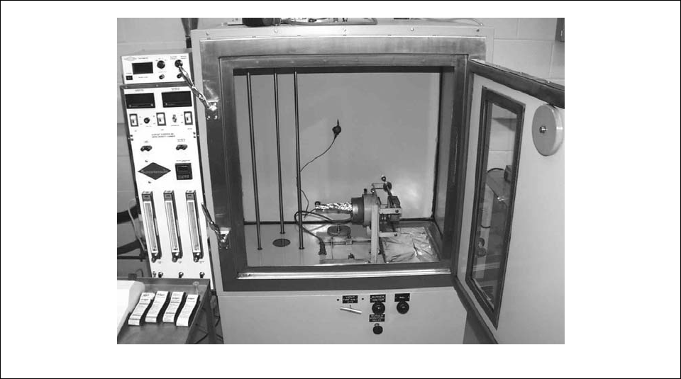
MIL-HDBK-17-1F

Volume 1, Chapter 6 Lamina, Laminate, and Special Form Characterization

6-83

vertical orientation parallel to the sample. The heater applies a flux of 25 kW/m

to the surface of the

sample.

Piloted ignition of the sample is accomplished with a multiple flamelet premixed propane/air burner.

The burner is located at the bottom of the sample. It is designed so that some of the flamelets will directly

impinge on the surface of the sample and some will be projected up parallel to the surface of the sample.

The apparatus is shown in Figure 6.6.18.3.1.

FIGURE 6.6.18.3.1 Photograph of ASTM E662 smoke chamber.

The sample is square in shape, measuring 2.99 x 2.99 in. (76 x 76 mm). The thickness may be var-

ied up to 25 mm. The sample is supported in a vertical orientation. The sample, holder, burner, and

heater are located inside a test enclosure which measures 2.99 ft. x 2.00 ft. x 2.99 ft. (914 x 610 x 914

mm) high. The enclosure is sealed except for ventilation openings at the bottom and top. The ventilation

openings are only open if the pressure inside the chamber goes negative.

Smoke obscuration is measured using a photometric system which transverses a vertical path from

the bottom to the top of the enclosure. An incandescent lamp is used for the light source. A photomulti-

plier tube is used as the receiver.

Values which are measured include externally applied flux and light transmitted. Values which are

then calculated include specific optical density.

6.6.18.3.2 NFPA 269 - Developing toxic potency data for use in fire hazard modeling

(Reference 6.6.18.3.2)

The National Fire Protection Association (NFPA) has adopted NFPA 269 for Use in Fire Hazard Mod-

eling. This is a small-scale test method that uses both analytical and bioassay techniques. In the test, a

specimen is subjected to electric spark ignition during exposure to a 50 kW/m

radiant flux for 15 minutes.

The smoke produced is collected for 30 minutes in a sealed chamber. The concentrations of CO, CO

and O

are measured over the test period, and a value for the concentration-time product (Ct) is calcu-

MIL-HDBK-17-1F

Volume 1, Chapter 6 Lamina, Laminate, and Special Form Characterization

6-84

lated by integration of the area under the concentration-time curves. Measurement of HCN, HCL, and

HBr is optional based on the material composition. The Ct product and the mass loss of the test speci-

men are used to calculate the Fractional Effective Dose (FED) for the test, and this value is used in a cal-

culation to predict the 30-minute LC

of the specimen. LC

is a measure of the lethal toxic potency. It is

the concentration of gas or smoke statistically calculated from concentration-response data to produce

lethality in 50% of test animals within a specified exposure and post exposure time. This predicted LC

then confirmed in a comparable test by exposing six rats to the smoke produced by a specimen sized to

produce the predicted LC

of the smoke in the exposure chamber. The number of rats which die during

the 30-minute exposure period and the subsequent 14 day post-exposure period determine the validity of

the predicted LC

. In this manner, it is possible to ensure that the monitored toxicants actually account

for the observed effects. The LC

value that is developed is for a pre-flashover fire and additional calcu-

lations are provided such that an LC

for a post-flashover fire is calculated. This correction factor is

based on the increased CO concentration that occurs during post-flashover fires that are ventilation con-

trolled.

6.6.18.4 Heat release test methods

In recent years, developments in fire research and understanding of fire dynamics have highlighted

the importance of heat release rate (HRR) as the primary fire hazard indicator. Fire hazard under a given

set of conditions of fuel load, geometric configurations, and ventilation conditions can be expressed in

terms of heat release rate and the fire hazard analysis should include the relevant fire response parame-

ter(s) of a material obtained from small scale heat release rate tests. The assessment of potential fire

hazard based on heat release rate measurements extends to composite materials also. The rate of heat

release, especially the peak amount, is the primary characteristic determining the size, growth, and sup-

pression requirements of a fire environment (References 6.6.18.4(a) and (b)).

6.6.18.4.1 ASTM E-1354 - Heat and visible smoke release rates for materials and products using an

oxygen consumption calorimeter

(Reference 6.6.18.4.1)

ASTM E-1354 measures the response of a small sample of material exposed to controlled levels of

radiant heating and is used to determine the heat release rates, ignitability, mass loss rates, effective heat

of combustion, and visible smoke development. Commonly referred to as the cone calorimeter, this

bench scale fire test method involves an application of the oxygen consumption principle and is sche-

matically shown in Figure 6.6.4.1. The oxygen consumption principle states that for most combustibles

there is a unique constant, 13.1 MJ/kg O

, relating the amount of heat released during a combustion reac-

tion and the amount of oxygen consumed from the air. Thus, using this principle, it is only necessary to

measure the concentration of oxygen in the combustion system along with the flow rate. The air-flow past

the specimen is generally set at 24 liter/s. This results in a highly fuel-lean combustion condition.

Specimens of a material or product to be tested are cut into a 3.94 x 3.94 in. (100 x 100 mm) size.

The thickness depends on the type of product tested and can range from .24 to 1.96 in. (6 to 50 mm).

The specimen edges are protected from burning, and the specimen can be oriented either horizontally or

vertically. The specimen is heated by an electric heater in the shape of a truncated cone, hence, the

name cone calorimeter. The irradiance to the specimen can be set to any desired value from zero to 110

kW/m

, but specific thermal insults of 25, 50, 75, and 100 kW/m

are required. These thermal insults cor-

respond to a small Class A fire, a large trash can fire, a significant fire, and an oil pool fire. Piloted ignition

of the specimen is provided by an electric spark. Since a uniform, controlled irradiance is provided, the

ignition times themselves, as measured, constitute a suitable test for ignitability. The specimen is

mounted on a load cell, and its mass, along with all other instrument data, is recorded to provide mass

loss rate data. The smoke measuring system is comprised of a He-Ne laser beam projected across the

exhaust duct. The monochromatic light is monitored by a solid-state detector. A second detector serves

as a reference to guard against effects of drift and of laser power fluctuations. The optical system is de-

signed to be self-purging and does not use optical windows. Full specification of test conditions requires

specifying the irradiance, the specimen orientation, the use of spark ignition, the test irradiance, and any

special specimen preparation techniques.

MIL-HDBK-17-1F

Volume 1, Chapter 6 Lamina, Laminate, and Special Form Characterization

6-85

The data derived from tests in the cone calorimeter constitute a very large set and can be analyzed in

a multitude of ways. The data reported include the following:

(a) Peak rate of heat release (kW/m

)

(b) Rates of heat release averaged over various time periods, starting with the time of ignition

(kW/m

)

combustion since the combustion is incomplete (as it is in real fires)

(d) Percent specimen mass lost (%)

(e) Time to ignition (s)

(f) Average smoke obscuration (m

/kg). Smoke production from a material has the rational units of

, representing the extinction cross-section of the smoke. This is normalized by the amount of

specimen mass lost (kg)

(g) Average yields of each of the measured gas species (kg/kg)

FIGURE 6.6.18.4.1 Schematic of ASTM E 1354.

6.6.18.4.2 ASTM E 906 – Heat and visible smoke release rates for materials and products

(Reference 6.6.18.4.2)

ASTM E 906 is based on a thermopile method where the temperature rise is used to determine the

heat release rate of materials. This thermopile method measures the heat release of materials at a radi-

ant heat flux of 35 kW/m

. The apparatus consists of a combustion chamber inside an insulated metal

box. The radiant source comprises four silicon carbide heating elements of nominal resistance of 1.4

ohms. Specimens are exposed to the radiant heater source inside the chamber at an irradiance of 35

kW/m

Samples are 59 x 59 in. (150x150 cm) in size and a minimum of three specimens are tested for each

material. The ignition is caused by a pilot flame from a methane burner placed above the specimen

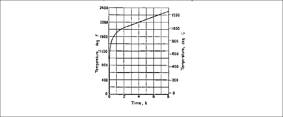
MIL-HDBK-17-1F

Volume 1, Chapter 6 Lamina, Laminate, and Special Form Characterization

6-86

holder. The total airflow rate through the apparatus is 40 liter/s airflow of which 10 liter/s passes through

the combustion chamber. The remaining 30 liter/s flows through the hollow wall section. The tempera-

tures of inflowing air and outflowing gases are measured with a thermopile consisting of 5 type K thermo-

couples. The hot junctions of the thermocouples are distributed along the diagonals of the stack above a

baffle plate. The increase in temperature of the gases exiting the stack with respect to the air tempera-

ture entering the combustion zone gives a measure of the heat release rate of the material.

6.6.18.5 Fire resistance test methods

The intensity and duration of a fire can vary over a wide range. It is important to have some under-

standing of the resistance of building assemblies to different fire threats in order to choose those which

more closely match the potential fire threat in a given compartment. Fire resistance here means the abil-

ity of a material to continue to serve its structural role during a fire (References 6.6.18.5(a) and (b)).

6.6.18.5.1 ASTM E-119 - Fire tests for building construction and materials

(Reference 6.6.18.5.1)

One test method for fire resistance is ASTM E-119, which uses what is often referred to as the stan-

dard time-temperature curve. Underwriters Laboratory utilizes this test method to provide fire ratings for

all assemblies used in building construction.

In this test, structural components are subjected to a heated furnace environment for the desired du-

ration. If the endpoint criteria are not reached prior to the end of the test period, the assembly is rated as

acceptable for that test period, e.g., 30 or 60 minutes. The furnace is heated in such a manner so that the

temperature inside the furnace follows a standard time-temperature curve. This curve, shown in Figure

6.6.18.5.1, is intended to relate to conditions in a fully developed room fire. Assemblies may be tested

with or without load. If the assembly is tested under load, the assembly is loaded to induce maximum

design stress levels calculated based on theory. Floor and roof assemblies and bearing walls are always

tested under load. In addition, a second specimen must be exposed to a hose stream to simulate manual

fire fighting and rapid cooling.

Sample sizes for this test are specified as follows: bearing walls and partitions, 9.3 m

nonbearing

walls and partitions, 9.3 m

; columns, 2.7 m; floors and roofs, 16.7 m

FIGURE 6.6.18.5.1 ASTM E-119 Time temperature curve.

MIL-HDBK-17-1F

Volume 1, Chapter 6 Lamina, Laminate, and Special Form Characterization

6-87

6.6.18.5.2 ASTM E-1529 - Determining effects of large hydrocarbon pool fires on structural members

and assemblies and UL 1709 - Rapid rise fire tests of protection materials for structural steel

(References 6.6.18.5.2(a) and (b)).

One of the distinguishing features of a post flashover fire is the rapid development of high tempera-

tures and heat fluxes that can subject exposed structural members to thermal shock much more readily

than they see in ASTM E-119. The ASTM E-1529 fire curves address this issue. The performance of

structural members and assemblies exposed to fire conditions resulting from large, free-burning fluid-

hydrocarbon-fueled pool fires is the focus of this test. The exposure scenario which is simulated by this

test is the condition of total, continuous engulfment of a member or assembly in the luminous flame area

of a large free-burning-fluid-hydrocarbon pool fire.

The test setup provides an average surface heat flux on all exposed surfaces of the test specimen of

158

± 8 kW/m

. This heat flux is attained within the first 5 minutes of test exposure and maintained for the

duration of the test. The test environment reaches a temperature of at least 1500°F (815°C) after the first

3 minutes of the test and remains between 1850°F and 2150°F (1010°C and 1176°C) at all times after the

first 5 minutes of the test. Because hydrocarbon pool fires often occur in outdoor environments, proce-

dures for accelerated weathering and aging tests are set forth to simulate weathering and aging in out-

door environments. Fire endurance ratings are given for the time period during which the assembly with-

stands the fire scenario without allowing the passage of flame or hot gases capable of igniting cotton

waste.

The temperature conditions described in UL 1709 (Standard for Rapid Rise Fire Tests of Protection

Materials for Structural Steel) are similar to those described above for ASTM E-1529. However, heat

fluxes described in UL 1709 (204

± 16 kW/m

) are higher than those described in ASTM E-1529 (158 ± 8

kW/m

). The UL 1709 fire curve rises to at least 1500°F (815°C) after the first 3 minutes of the test and is

between 1850°F (1010°C) and 2150°F (1180°C) at all times after the first 5 minutes of the test. In con-

trast to ASTM E-1529 and UL 1709, the ASTM E-119 fire curve rises to only 1000°F (538°C) at the end of

the first 5 minutes, and to 1700°F (927°C) at the end of 60 minutes.

6.7 ELECTRICAL PROPERTY TESTS

6.7.1 Introduction

In certain applications, the electrical properties of a composite are important. The properties that are

of interest include dielectric constant, dielectric strength, volume resistivity, surface resistivity, are resis-

tance, dissipation and loss factors. The values can be affected by temperature and environment, as well

as the type of curing agent, filler, and fiber used in the composite. The following ASTM test methods can

be used for determining the electrical properties of polymer matrix composite laminae and laminates:

ASTM D 149 "Standard Test Method for Dielectric Breakdown Voltage and Dielectric Strength of Solid

Electrical Insulating Materials at Commercial Power Frequencies". Method for determining the dielec-

tric strength of solid insulating materials.

ASTM D 150 "Standard Test Method for A-C Loss Characteristics and Permittivity (Dielectric Con-

stant) of Solid Electrical Insulating Materials". Method used for determining the relative permittivity,

dissipation factor, loss index, power factor, phase angle, and loss angle of solid insulating materials

when the standards are lumped impedances.

ASTM D 495 "Standard Test Method for High-Voltage, Low-Current, Dry Arc Resistance of Solid Elec-

tric Insulation". This test method is intended for preliminary screening of material and should not be

used in material specifications.

ASTM D 2303 "Standard Test Methods for Liquid-Contaminant, Inclined Plane Tracking and Erosion

of Insulating Materials". Test methods for the quantitative evaluation of the relative ability of insulating

MIL-HDBK-17-1F

Volume 1, Chapter 6 Lamina, Laminate, and Special Form Characterization

6-88

materials to withstand the action of electrical discharges on the surface, similar to what may occur in

service under the influence of dirt and moisture condensed from the atmosphere.

6.7.2 Electrical permittivity

This section is reserved for future use.

6.7.3 Dielectric strength

This section is reserved for future use.

6.7.4 Magnetic permeability

This section is reserved for future use.

6.7.5 Electromagnetic interference

This section is reserved for future use.

6.7.6 Electrostatic discharage

This section is reserved for future use.

6.8 STATIC UNIAXIAL MECHANICAL PROPERTY TESTS

6.8.1 Introduction

Section 6.8 discusses test methods for determining the static uniaxial mechanical properties of lami-

nated composites. The purpose of this section is to provide brief commentaries on the most commonly

used methods, to alert the reader to the limitations of the various methods, and to encourage uniformity in

the use of standard test methods with the ultimate goal of combinability of experimental data obtained

from multiple sources. The reader is referred to Chapter 8 for statistical data analysis requirements for

reporting of data to MIL-HDBK-17.

The section reflects the current dynamic state of test methods development for composite materials.

Many of the methods were originally developed for testing of reinforced plastics, and modifications have

been (or are being) made for applicability to advanced composites. In recent years there has been a ten-

dency for users to unilaterally modify existing standards without a formal standardization process, leading

to uncontrolled test results. In general, these modified standards are not discussed in Section 6.8 except

where a specific modification is in common use, and where discussion of the technique is deemed con-

structive. The test methods included are representative of procedures used in the composite materials

industry, and were selected after review of standards documents and user material specifications. Spe-

cific test methods may cover lamina-level testing, laminate-level testing, or both, depending upon the test

method. The scope of each test method is discussed in the appropriate section.

It is important to make a distinction between methods that are discussed in Section 6.8, and methods

for data submittal to MIL-HDBK-17:

• Test methods used by contractors are agreed upon with customers and/or certifying agencies.

Section 6.8 reviews many methods in order to provide the reader with awareness of the broad

range of procedures in common use. Some of these have been formally standardized (ASTM

and other standards) and some are "common practice" methods. Some have distinct limitations,

and these are indicated as a matter of information. Mention or omission of a particular method

does not, of itself, require or restrict usage. Specific methods are included to allow the user to

MIL-HDBK-17-1F

Volume 1, Chapter 6 Lamina, Laminate, and Special Form Characterization

6-89

perform tests consistent with industry practice; however, inclusion of these standards should not

be considered an endorsement of any standard or organization by MIL-HDBK-17.

• When submitting data to MIL-HDBK-17 for consideration for inclusion in Volume 2 of the Hand-

book, specific methods must be used. Tables at the end of most subsections of 6.8 indicate

which methods are acceptable for such submittals. These methods have been chosen in accor-

dance with the criteria given in Section 2.5. Readers are encouraged to also use these methods

in contract and internal work to promote standardization.

When selecting and using a particular mechanical strength test method, the importance of obtaining

the proper failure mode cannot be overemphasized. While universal definitions of "proper" and "valid"

have not been established for most types of tests, further analysis must be employed when unexpected or

questionable modes are observed or suspected. If the type of failure is different from what is expected

from the test, the data may not represent the property being evaluated. Furthermore, if the failure mode

varies within a group of specimens, statistical analysis of the resulting data will not be meaningful due to

the introduction of an additional source of variability not related to the property being tested. Therefore, it

is crucial that failure modes be reported, and that data be disqualified and discarded when analysis has

indicated an unacceptable mode.

It should be noted that failure mode analysis is not necessarily limited to physical examination of the

failed test specimens. Other evidence might be obtained from review of additional factors such as:

1. Bending curves from back-to-back strain gage data

2. A check of test machine and/or test fixture alignment

3. A review of the exact procedure used to install and properly align the specimens in the test fixture

4. A check for possible damage to, or malfunction of, the test fixture

ASTM has begun to incorporate failure mode examples and codes into its standard test methods. For

example, the 1993 revision of ASTM D 3039 (Standard Test Method for Tensile Properties of Polymer Ma-

trix Composite Materials) depicts nine types of failures of the specimen, and defines a three-character

coding system that describes various failures. The first letter of the code identifies the type of failure (an-

gled, grip, delamination, etc.), the second indicates the area of the failure (gage, at grip, etc.), and the

third denotes the failure location (top, bottom, middle, etc.). In the particular case of tension testing, a

failure of the tab or tab adhesive would be an unacceptable mode since the ultimate tensile strength of

the laminate was not measured.

Rather than duplicate failure mode examples within the subsections of Section 6.8, the reader is ad-

vised to be conscientious regarding the documentation of failure modes, and to refer to examples pro-

vided within specific test methods where such examples exist.

6.8.2 Tensile properties

In-Plane Tensile Properties:

Lamina

, ,

εν

, ,

εν

Laminate

, ,

εν

, ,

εν

MIL-HDBK-17-1F

Volume 1, Chapter 6 Lamina, Laminate, and Special Form Characterization

6-90

Out-of-Plane Tensile Properties:

Lamina

, , ,

ενν

Laminate

, , ,

ενν

6.8.2.1 Overview

The basic physics of most tensile test methods are very similar: a prismatic specimen with a straight-

sided gage section is gripped at the ends and loaded in uniaxial tension. The principal differences be-

tween these tensile test specimens are the specimen cross-section and the load-introduction method.

The cross-section of the specimen may be rectangular, round, or tubular; it may be straight-sided for the

entire length (a “straight-sided” specimen) or width- or diameter-tapered from the ends (a larger area) into

the gage section (a smaller area).

Straight-sided specimens may, in some cases, utilize tabbed load ap-

plication points.

There are three notable exceptions to the uniaxially loaded prismatic specimen: 1) a sandwich beam

test that relies upon gross flexure of a sandwich beam to create an in-plane stress state in the facesheets,

making the tensile facesheet, in effect, the specimen; 2) a ring test that applies, via a fixture, a diametrical

expansion (or an approximation of such) to a narrow, high radius-to-thickness ratio ring, creating a mem-

brane (in-plane) tensile stress in the ring; and 3) a solid-laminate curved beam test that applies, via a fix-

ture, an opening bending moment, producing a through the thickness tensile stress in the bend region.

While there are a number of existing or developing standards for in-plane tensile properties of lami-

nated materials, this is not the case for out-of-plane properties. Test methods potentially suitable to be-

come standards for through the thickness tensile properties of laminates have only recently begun to re-

ceive substantial attention, and so are relatively immature.

By changing the specimen configuration, many of the tensile test methods are able to evaluate differ-

ent material configurations, including unidirectional laminates, woven materials, and general laminates.

However, some specimen/material configuration combinations are more robust (less sensitive to speci-

men preparation and testing variations) than others. The least robust (most user-sensitive) configuration

is the unidirectional specimen. As an example, fiber/load misalignment in a 0° unidirectional specimen,

which can occur due to either specimen preparation or testing problems, or both, can reduce strength as

much as 30% due to an initial 1° misalignment. This specimen is also very sensitive to load-introduction

upsets and requires a high degree of laboratory sophistication, both in specimen preparation as well as

testing, to achieve satisfactory results. And bonded end-tabs, which were introduced in the late 1960’s to

minimize load-introduction problems in high-strength unidirectional materials, can actually cause prema-

ture specimen failure (even in non-unidirectional specimens), if not applied and used precisely and with

great art. Since most 0° unidirectional specimens fail with an explosive shatter that obscures the true fail-

ure mode, physical evidence of poor testing/specimen preparation practices is usually unavailable.

These difficulties with the testing of unidirectional materials have led to the increased use of a much

more robust [90/0]

-type laminate specimen (also known as the “crossply” specimen). From the laminate

strength of a crossply specimen (when the lamina elastic properties are known), the equivalent unidirec-

tional

lamina strength can be derived, using the procedure discussed in Section 2.4.2. When previ-

ously undocumented improvements in testing technique are combined with use of crossply test speci-

mens, much simpler untapered tabs, or even tabless specimens, are now feasible, allowing laboratories

that are generally qualified, but inexperienced in unidirectional testing, to produce results equivalent to the

best attainable unidirectional data. While unidirectional testing is still performed, and in certain cases may

be preferred or required, a straight-sided, tables, [90/0]

-type specimen is now generally believed to be

the lowest cost, most reliable configuration for lamina tensile testing of unidirectional materials. This

straight-sided tabless configuration also works equally well for non-unidirectional material forms and for

Though there have been many different types of tapered specimens, they are often called, as a class, Αdogbone≅ specimens.

MIL-HDBK-17-1F

Volume 1, Chapter 6 Lamina, Laminate, and Special Form Characterization

6-91

other general laminates. Another advantage is that, unlike with 0° unidirectional specimens, [90/0]

-type

specimen failures do not usually mask indicators of improper testing/specimen preparation practices.

6.8.2.2 In-plane tension test methods

6.8.2.2.1 Straight-sided specimen tension tests

1) ASTM D 3039/D 3039M, Standard Test Method for Tensile Properties of Polymer Matrix Compos-

ites

2) ISO 527, Plastics --- Determination of Tensile Properties

3) SACMA RM 4, Tensile Properties of Oriented Fiber-Resin Composites

4) SACMA RM 9, Tensile Properties of Oriented Cross-Plied Fiber-Resin Composites

5) ASTM D 5083, Standard Test Method for Tensile Properties of Reinforced Thermosetting Plastics

Using Straight-Sided Specimens

ASTM Test Method D 3039/D 3039M (Reference 6.8.2.2.1(a)), originally released in 1971, is the

original standard test method for straight-sided rectangular specimens. As a result of a major re-write of

D 3039, approved in 1993, tabs were made optional, and a significant number of previously ambiguous,

undocumented, and/or optional test and reporting parameters were clarified, documented, and/or made

mandatory. ISO 527 (Reference 6.8.2.2.1(b)) parts 4 and 5 (currently in the draft international standard

phase) and the two SACMA (Suppliers of Advanced Composite Materials Association) tensile test meth-

ods, SRM 4 (Reference 6.8.2.2.1(c)) and SRM 9 (Reference 6.8.2.2.1(d)) are substantially based on

ASTM D 3039 and, as a result, quite similar.

While there are still a number of minor differences between ASTM D 3039 and ISO 527, there is a

coordinated effort underway to harmonize ASTM D 3039 and ISO 527 and make them technically equiva-

lent. SRM’s 4 and 9, while originally intended to be restricted subsets of ASTM D 3039, deviate from

ASTM D 3039 enough that they are not exactly equivalent test methods; an ASTM/SACMA harmonization

effort is being discussed but has not yet begun.

The last of the straight-sided test methods, ASTM

D 5083 (Reference 6.8.2.2.1(e)), is the straight-sided equivalent of the ASTM D 638 dogbone tension test

for plastics (discussed in Section 6.8.2.2.3). While ASTM D 5083 is conceptually similar to ASTM D 3039,

D 5083 was not developed for use with advanced composites, and therefore, cannot be recommended.

In all of these test methods, a tensile stress is applied to the specimen through a mechanical shear

interface at the ends of the specimen, normally by either wedge or hydraulic grips. The material response

is measured in the gage section of the specimen by either strain gages or extensometers, and the elastic

material properties subsequently determined.

End tabs, if used, are intended to distribute the load from the grips into the specimen with a minimum

of stress concentration. A schematic example of an appropriate failure mode of a multidirectional lami-

nate using a tabbed tensile specimen is shown in Figure 6.8.2.2.1(a). However, design of the tabs re-

mains somewhat of an art, and an improperly designed tab interface will produce an unacceptable propor-

tion of failures near the tab and result in very low specimen strengths. For this reason a single standard

tab design has not been mandated by ASTM, although, when tabs are necessary, the easier-to-apply, less

expensive, unbeveled 90° tabs are preferred if the results are acceptable. Recent comparisons confirm

that success of a tab design is more dependent on use of a sufficiently ductile adhesive than on the tab

angle. An unbeveled tab applied with a ductile adhesive will outperform a tapered tab that has been ap-

plied with a insufficiently ductile adhesive. Adhesive selection is therefore most critical to bonded tab use.

The simplest way to avoid bonded tab problems is to not use them. Many laminates (mostly non-

unidirectional) can be successfully tested without tabs, or with friction tabs. An example of a high-strength

carbon/epoxy material being tested in an untabbed, [90/0]

-type laminate configuration using an emery

ASTM D 3039 contains bending and failure mode restrictions not present in SRM=s 4 and 9, and is different in other respects like

thickness measurement, conditioning, and data reporting. ASTM D 3039 is also significantly more detailed than SRM=s 4 and 9.

The sum of these differences may produce a different test result.

MIL-HDBK-17-1F

Volume 1, Chapter 6 Lamina, Laminate, and Special Form Characterization

6-92

cloth interface in finely serrated wedge grips is shown in Figure 6.8.2.2.1(b). Flame-sprayed unserrated

grips have also been successfully used in tabless tension testing.

FIGURE 6.8.2.2.1(a) Typical tension failure of multi-directional laminate using a tabbed specimen.

Other important factors that affect tension testing results include control of specimen preparation,

specimen design tolerances, control of conditioning and moisture content variability, control of test ma-

chine-induced misalignment and bending, consistent measurement of thickness, appropriate selection of

transducers and calibration of instrumentation, documentation and description of failure modes, definition

of elastic property calculation details, and data reporting guidelines. These factors are described in detail,

and controlled, where appropriate, by ASTM D 3039/D 3039M. While ISO 527 parts 4 and 5 and SRM’s 4

and 9 are similar to ASTM D 3039/D 3039M in most respects, they do not provide the same degree of

guidance or control as ASTM D 3039. For this reason ASTM D 3039 is preferred.

In summary, with proper attention to detail and reasonable care the straight-sided specimen test is

generally straightforward and gives good results. However, test parameters must be properly selected for

the material and configuration under test, which requires training and experience.

Limitations of the straight-sided specimen tensile test:

Bonded Tabs: The stress field near the termination of a bonded tab is significantly three-dimensional,

and critical stresses tend to peak at this location. Design of bonded tabs for the purpose of minimizing

peaking stresses is not well-understood and is material and configuration dependent; improperly de-

signed tabs can significantly degrade results. As a result, tables or unbonded tabbed configurations are

becoming more popular, when the resulting failure mode is appropriate.

Specimen Design: There are, particularly within ASTM D 3039, a large number of specimen design op-

tions included in the standard, needed to cover the wide range of material systems and lay-up configura-

tions within the scope of the test method. These options can be very confusing to the novice, and can

lead to the selection of an inappropriate specimen design that negatively affects test results.

Specimen Preparation: Specimen preparation is very important to the test results. While this can proba-

bly be said to be true for almost all composite mechanical tests, it is particularly important for unidirec-

tional tests, and unidirectional tension tests are no exception. Fiber alignment, control of specimen taper,

and specimen machining (while maintaining alignment) are the most critical steps. For very low strain-to-

failure material systems or test configurations, like the 90° unidirectional test, flatness is also particularly

important. Edge machining techniques (avoiding machining-induced damage) and edge surface finish

are also particularly critical to strength results from the 90° unidirectional test.

MIL-HDBK-17-1F

Volume 1, Chapter 6 Lamina, Laminate, and Special Form Characterization

6-93

FIGURE 6.8.2.2.1(b) Tension testing of untabbed specimen using an emery-cloth gripping interface.

MIL-HDBK-17-1F

Volume 1, Chapter 6 Lamina, Laminate, and Special Form Characterization

6-94

6.8.2.2.2 Filament-wound tubes

ASTM Standard Test Method D 5450/D 5450M, Transverse Tensile Properties of Hoop Wound Poly-

mer Matrix Composite Cylinders

ASTM D 5450 describes a test for 90° tensile properties, specifically for a hoop-wound unidirectional

cylinder. This test method is discussed in more detail in Section 6.12.1 on test methods for filament

wound materials.

6.8.2.2.3 Width tapered specimens:

1) ASTM Standard Test Method D 638, Tensile Properties of Plastics

2) SAE AMS “Bowtie” Tension Specimen

ASTM Test Method D 638 (Reference 6.8.2.2.3(a)), developed for and limited by scope to use with

plastics, uses a flat, width-tapered tension specimen with a straight-sided gage section. Despite its heri-

tage, this specimen has also been evaluated on and applied to composite materials. The specimen taper

is accomplished by a large cylindrical radius between the wide gripping area at each end and the nar-

rower gage section, resulting in a shape that justifies the specimen nickname of the “dogbone” specimen.

The taper makes the specimen particularly unsuited for testing of 0° unidirectional materials, since about

half of the gripped fibers terminate prior to the gage section, resulting in failure by splitting at the radius

due to inability of the matrix to shear the load from terminated fibers into the gage section.

While the ASTM D 638 specimen configuration has sometimes been successfully used for fabric rein-

forced composites and with general non-unidirectional laminates, some material systems remain sensitive

to the stress concentration at the radius. While, for its intended use with plastics, the specimen is molded

to shape, for laminated materials the specimen must be machined, ground, or routed to shape. The

specimen also has the drawback of having a relatively small gage volume and is poorly suited for charac-

terization of coarse weaves with repeating units larger than the gage width of 0.25-0.50 in. (6.4-13 mm).

The standardized procedure, due to the intended scope, does not adequately cover the testing

parameters required for advanced composites.

The bowtie tension test specimen, so-called because of its planform shape with a reduced cross-

section, is similar in many respects to the ASTM D 638 specimen, though it has never been released as a

standard test method. The bowtie specimen has achieved indirect standardization through use in several

SAE AMS composite material (fabric-based) specifications

. It is also still contained within a number of

existing corporate internal material specifications for fabric-based materials, though it is rarely used now

in new material specifications. With the geometric similarity to the ASTM D 638 specimen come a similar

set of limitations and restrictions. The shape fundamentally restricts use to fabric reinforced materials

and/or non-unidirectional laminates. Specimen preparation is extremely important since the reduced

cross-section is prepared by machining, routing, or grinding, and both surface finish of the edge and ma-

chining of the tangent radii at the transition region to the reduced area are critical. The specimen also

does not work well with coarse fabrics, since the gage section is only 0.5-in. (13 mm) wide.

To its credit, the bowtie specimen is reportedly somewhat less sensitive to failures in the transition

section than the D 638 specimen, and has also been employed as a resource of last resort, particularly

when the severity of non-ambient test environments creates otherwise difficult gripping problems for

straight-sided specimens.

Other width-tapered specimen configurations have been proposed, but to date each has been shown,

after study, to have at least one shortcoming that renders the method undesirable for general application,

and so will not be further discussed.

The four known SAE specifications containing the bowtie coupon at the time of this writing were: AMS 3844A (Reference

6.8.2.2.3(b)), AMS 3845A, AMS 3847B, and AMS 3849A. Only the first, as an example, is completely referenced.

MIL-HDBK-17-1F

Volume 1, Chapter 6 Lamina, Laminate, and Special Form Characterization

6-95

Limitations of the width-tapered tension tests for advanced composites:

Standardization: While the ASTM D 638 test is standardized, it was not developed for advanced com-

posites, and is primarily applicable to relatively low modulus, unreinforced materials, or low reinforcement

volume materials incorporating randomly oriented fibers. The bowtie test is standardized only in the

sense of continued use in a limited number of SAE AMS material specifications. It has not been stan-

dardized for general use.

Specimen preparation: Special care is required to machine the taper into a laminated coupon.

Cost: Specimen fabrication is more expensive than untabbed straight-sided coupons.

Stress state: The radius transition region can dominate the failure mode and result in reduced strength

results. The width-tapered specimen is not suitable for unidirectional laminates, and is limited to fabrics or

non-unidirectional laminates when gage section failures can be attained.

Limited gage section volume: The limited gage width makes it unsuitable for coarse fabrics.

6.8.2.2.4 Split-disk ring tension test

ASTM Standard Test Method D 2290, Apparent Tensile Strength of Ring or Tubular Plastics and Rein-

forced Plastics by Split Disk Method

Procedure A (Procedures B and C apply only to plastics) of ASTM D 2290 (Reference 6.8.2.2.4) loads

a hoop-wound narrow ring using a split-disk loading fixture that applies a hoop-direction tensile stress to

the test ring. This test method was developed in the early years of composites, primarily for tensile prop-

erties of filament wound materials. It has long since been superseded by more reliable and more repre-

sentative test methods. The disadvantages will not be dwelled upon, but include the material

form/process limitation, the presence of a unaccounted bending moment at the fixture split, the extremely

small gage volume, and the inability to monitor strain response. This test is not recommended for MIL-

HDBK-17 data, but it still sees some limited usage as a quality control test in the filament winding indus-

try.

6.8.2.2.5 Sandwich beam test

ASTM Standard Test Method C 393, Flexural Properties of Flat Sandwich Constructions

The sandwich beam test, shown schematically in Figure 6.8.2.2.5 is standardized as ASTM C 393

(Reference 6.8.2.2.5). While primarily intended as a flexure test for sandwich core shear evaluation, the

scope also allows use for determination of facing tensile strength. While this use is not well documented

within the test method, it has been used for tension testing of composite materials, particularly for 90°

properties of unidirectional materials, or for fiber-dominated testing in extreme non-ambient environments.

An example of practical use of this test method for 90° unidirectional tape properties follows. A piece

of 0.5-in. thick, 1/8-in. cell, 8.1 lbm/ft

(13 mm thick, 3 mm cell, 130 kg/m

) aluminum honeycomb core is

bonded to the test laminate using a suitable adhesive. A compressive faceskin is also bonded to the

other side of the core, normally during the same bonding step. To minimize thermal expansion problems

from dissimilar materials, the compressive faceskin is often chosen to be of the same material and orien-

tation, but at twice the thickness of the tensile faceskin to assure failure in the tensile faceskin. The test

specimen is then cut with a wet-diamond saw from the sandwich laminate. Specimen dimensions are 1

inch (25 mm) wide and 8 inch (200 mm) long, with the core ribbon direction aligned with the length of the

specimen. The test setup uses a support span of 7 inch (180 mm) and a four-point loading span of 3 inch

(76 mm). The load is both applied and reacted at all points using 1-inch (25 mm) square, 1/8-inch (3 mm)

thick rubber pads, which are in turn each loaded by a 1/4-inch (6 mm) thick steel loading plate of the

same area. The load is applied to each loading plate via a 1/2-inch (13 mm) diameter steel roller that

rides in a transverse slot in the loading plate. This loading mechanism distributes the load into the beam

MIL-HDBK-17-1F

Volume 1, Chapter 6 Lamina, Laminate, and Special Form Characterization

6-96

and prevents out-of-plane crushing of the core. The specimen and loading fixturing are shown schemati-

cally in Figure 6.8.2.2.5.

FIGURE 6.8.2.2.5 Schematic of sandwich beam test coupon and fixturing, for 90°

unidirectional tensile testing of laminated materials.

This test specimen is claimed by some to be less susceptible to handling and specimen preparation

damage than D 3039-type 90° specimens, resulting in higher strengths and less test-induced variation.

However, the one-sided environmental conditioning of this specimen is a problem, since the required con-

ditioning times are longer by a factor of four or more, and such conditioning can create adhesive bond

failures. Adhesive selection is, therefore, important and masking of the adhesive from the environmental

conditioning may be required. In such cases, conditioning travelers are required that must be twice the

test skin thickness in order to simulate the single-sided exposure of the specimen itself.

Limitations of the sandwich beam test for tensile properties:

Cost: Specimen fabrication is relatively expensive.

Stress State: The effect on the stress state of the sandwich core has not been studied in tension, and

could be a concern.

Standardization: While this test technically is standardized, its practical application and limitations are

not well studied or documented.

Conditioning: Conditioning is more difficult, as described above.

MIL-HDBK-17-1F

Volume 1, Chapter 6 Lamina, Laminate, and Special Form Characterization

6-97

6.8.2.3 Out-of-plane tensile test methods

6.8.2.3.1 Introduction

There are currently no published standards for out-of-plane tensile test methods specifically relating

to composites. Two basic approaches are presently in use, or being studied, by the aerospace industry

include: direct out-of-plane loading of a laminated specimen bonded between two fixture blocks (based on

modifications to similar non-composite test methods) and indirect out-of-plane loading of a curved beam.

Both concepts are being considered for possible standardization in composite use by ASTM.

6.8.2.3.2 Direct out-of-plane loading adaptations of ASTM C 297/C 633/D 2095

1) using square cylinder loading blocks, or

2) using circular cylinder loading blocks

Three similar ASTM standard test methods already used for out-of-plane loading of other material

systems have been adapted to composites: ASTM C 297 (Reference 6.8.2.3.2(a)), ASTM C 633 (Refer-

ence 6.8.2.3.2(b)), and ASTM D 2095 (Reference 6.8.2.3.2(c)). In the adaptations to composites a lami-

nated specimen is bonded to cylindrical metal loading blocks which are pulled in the out-of-plane direction

by a tensile test machine. The metal loading cylinders are either square or circular. The square speci-

mens are typically 2-in. (50 mm) in width, while the circular specimens range in diameter from 0.8-in. to 2-

in (20-50 mm). Strength is determined simply by dividing maximum load prior to failure by the specimen

gage area.

If the specimen is sufficiently thick, strain gages may be used to determine elastic modulus. A thick

specimen may also allow a reduced diameter gage section, which may be required if the out-of-plane

strength exceeds the bond strength of the specimen/loading-block interface.

It has been argued by some that a circular specimen achieves a more uniform stress distribution

(lower stress concentration). However, either configuration is extremely sensitive to specimen prepara-

tion factors, especially surface finish of the specimen edge and alignment of the load and loading blocks.

Two typical specimen configurations are shown in Figure 6.8.2.3.2(a).

Each of the ASTM test methods uses a different method of introducing the load to the loading blocks.

ASTM C 297 uses what is essentially a universal joint at each end. ASTM C 633 (circular only) applies a

thread to the opposite end of each loading block and depends upon test machine alignment to eliminate

bending. ASTM D 2095 uses a fixture that eliminates one of the bending degrees of freedom at one end,

and the other bending degree of freedom at the other end. These three approaches are shown in Figures

6.8.2.3.2 (b-d).

Limitations of the direct out-of-plane tensile test methods:

Standardization: Despite the existence of three similar standards intended for use on other material sys-

tems, there is currently no standard for application of the methodology to laminated composites. This ap-

proach is still being studied.

Cost: Due to tight tolerances required for repeatable representative data, specimen preparation is rela-

tively expensive.

Specimen preparation: Results are extremely sensitive to alignment of the loading blocks during bond-

ing, as well as the machining quality and surface finish of the laminate edges. This implies that the lami-

nate itself must be flat. An additional consideration is CTE-mismatch induced thermal stresses caused

by a significant difference between the laminate in-plane CTE and the end-block CTE. This is especially

important during end-block bonding, as well as during non-ambient testing.

MIL-HDBK-17-1F

Volume 1, Chapter 6 Lamina, Laminate, and Special Form Characterization

6-98

FIGURE 6.8.2.3.2(a) Two typical direct out-of-plane tensile specimen configurations.

MIL-HDBK-17-1F

Volume 1, Chapter 6 Lamina, Laminate, and Special Form Characterization

6-99

FIGURE 6.8.2.3.2(b) The ASTM C 297 loading fixture.

MIL-HDBK-17-1F

Volume 1, Chapter 6 Lamina, Laminate, and Special Form Characterization

6-100

FIGURE 6.8.2.3.2(c) ASTM C 633 end-blocks.

MIL-HDBK-17-1F

Volume 1, Chapter 6 Lamina, Laminate, and Special Form Characterization

6-101

FIGURE 6.8.2.3.2(d) The ASTM D 2095 loading fixture.

MIL-HDBK-17-1F

Volume 1, Chapter 6 Lamina, Laminate, and Special Form Characterization

6-102

6.8.2.3.3 Curved beam approach to out-of-plane tensile strength

This technique takes advantage of the out-of-plane tensile loading induced in the elbow of a curved

laminate beam subjected to an opening moment. Several researchers have published investigations of

different variations of this technique, exploring specimen size, specimen shape (90° small radius or “C”-

shaped), and loading methods (attachment fixture used to apply an opening tensile load, or a four-point

flexural fixture) (e.g., Reference 6.8.2.3.3). Typical specimen configurations are conceptually illustrated

by Figure 6.8.2.3.3.

Limitations:

Standardization: Currently non-standard, although it is being evaluated for possible standardization by

ASTM D-30.

Inconsistent results: Early investigations indicate results are strongly geometry and size dependent.

Material response: Unlike the direct out-of-plane loading method with a thick laminate, the specimen

cannot be instrumented for out-of-plane strain and therefore modulus cannot be determined.

FIGURE 6.8.2.3.3 Curved beam loading approaches.

6.8.2.4 Tension test methods for MIL-HDBK-17 data submittal

Data produced by the following test methods (Table 6.8.2.4) are currently being accepted by MIL-

HDBK-17 for consideration for inclusion in Volume 2.

MIL-HDBK-17-1F

Volume 1, Chapter 6 Lamina, Laminate, and Special Form Characterization

6-103

TABLE 6.8.2.4 Tension test methods for MIL-HDBK-17 data submittal.

Symbols

Fully Approved, In-

terim, and Screening

Data

Screening

Data Only

LAMINA PROPERTIES

0° In-Plane Strength

D 3039, SRM 4, SRM 9

(crossply only)

---

0° In-Plane Modulus, Poisson's Ratio

D 3039, SRM 4 ---

90° In-Plane Strength

D 3039, SRM 4,

D 5450

---

90° In-Plane Modulus

D 3039, SRM 4,

D 5450

---

Out-of-Plane Strength

(no recommendation) ---

Out-of-Plane Modulus, Poisson's Ratios

, ,

νν

(no recommendation) ---

LAMINATE PROPERTIES

x In-Plane Strength

D 3039 ---

x In-Plane Modulus, Poisson's Ratio

D 3039 ---

y In-Plane Strength

D 3039 ---

y In-Plane Modulus

D 3039 ---

Out-of-Plane Strength

(no recommendation) ---

Out-of-Plane Modulus, Poisson's Ratios

, ,

νν

(no recommendation) ---

MIL-HDBK-17-1F

Volume 1, Chapter 6 Lamina, Laminate, and Special Form Characterization

6-104

6.8.3 Compressive properties

In-Plane Compressive Properties

Lamina

, ,

εν

Laminate

, ,

εν

6.8.3.1 Overview

The compressive response of composite materials has been the subject of research efforts and test

programs since the early 1970’s. Yet there remain numerous methods in use for testing composites in

compression and no consensus as to which should be recommended.

Compression tests are conducted on composite materials, utilizing appropriate instrumentation, to

determine compressive modulus, Poisson's ratio, ultimate compressive strength and/or strain-at-failure.

These properties are determined through use of test fixturing that is typically designed 1) to introduce a

uniform state of uniaxial stress in the specimen test section, 2) to minimize stress concentrations, 3) to be

as simple to use and fabricate as possible. and 4) to minimize specimen volume. Compressive data are

used for various purposes including research, quality control and generation of design allowables.

Measures of quality for a particular compressive test method include low coefficients of variation for

strength and modulus, as well as the value of the modulus obtained relative to that from other compres-

sion test methods. While relative compressive strength is also often used as another measure of com-

pression test quality, the inherent differences in compression response between the different compression

tests mean that the test fixture, the resulting failure modes, and the application must be considered along

with the resulting strengths. Compressive strengths from some methods may be considered "artificially

high" due to fixture/coupon restraints that may suppress certain "real world" failure modes. Typically, fix-

tures are designed to induce failure in the test section and to intentionally inhibit some failure modes such

as end brooming and column buckling that, if permitted to occur, would result in "artificially low" strengths.

This tradeoff between just enough restraint versus too much restraint, and artificially high versus artifi-

cially low compressive strength, is the reason for the myriad of possible test methods and the lack of

agreement on one acceptable method. There are differences of opinion on how to balance these trade-

offs. Final selection of a compressive test method depends on the goals of the testing program.

The measured compressive strength for a single material system has been shown to differ when de-

termined by different test methods. Other parameters found to be significant contributors to the variations

in results include fabrication practices, control of fiber alignment, improper and/or inaccurate specimen

machining, improper tabbing procedures if tabs are used, poor quality of the test fixture, improper place-

ment of the specimen in the test fixture, improper placement of the fixture in the testing machine, and an

improper test procedure.

A review of the numerous compression test methods available reveals they can be broadly classified

into three groups: 1) those that introduce load into the specimen test section through shear, 2) those that

introduce load into the specimen test section through direct compression (end-loading), and 3) those that

introduce load into the specimen test section through a combination of end-loading and shear. The two

compressive test methods for fiber-reinforced composites currently published by ASTM Committee D-30

in D 3410-95 (Reference 6.8.3.1(a)) and the one method in D 5467-97 (Reference 6.8.3.1(b)) introduce

load into the test section of the specimen primarily by shear. ASTM D 695 (Reference 6.8.3.1(c)),

MIL-HDBK-17-1F

Volume 1, Chapter 6 Lamina, Laminate, and Special Form Characterization

6-105

SACMA SRM-1R-94 (Reference 6.8.3.1(d)), and SRM-6-94 (Reference 6.8.3.1(e)) utilize end loading.

ASTM D 6484 (Reference 6.8.3.1(f)) is a combined loading test method.

Compressive test methods can be further classified as having a supported or an unsupported test

section. An unsupported test section is defined as one with nothing in contact with the surfaces of the

specimen in the test section throughout the entire compression test. A supported test section is one with

support on the specimen faces and/or edges in the test section provided by the test fixture or ancillary

equipment. All of the test methods discussed in this section utilize specimens with unsupported test sec-

tions, with the exception of ASTM D 5467, the Sandwich Beam method. A more complete discussion of

compression test methodology and a description of test methods not covered here can be found in Refer-

ences (6.8.3.1(g ) - (l)).

6.8.3.2 In-plane compression tests

The in-plane compressive test methods described below are typically used to generate the ultimate

compressive strength, strain-at-failure, modulus, and Poisson’s ratio of axially or transversely loaded uni-

directional composite specimens, over a typical thickness range of 0.040 to 0.400 in. (1 to 10 mm). With

the exception of the D 5467 (sandwich beam) method, all of the test methods discussed below will also

accommodate specially orthotropic laminates, including [0/90]

style laminates. The testing of [0/90]

laminates has become a particularly popular means of eliminating specimen- and fixture-related sensitivi-

ties associated with the use of unidirectional specimens. If lamina compressive data are desired from

[0/90]

laminates, data reduction procedures are required. A discussion of the use of [0/90] laminates for

determining lamina properties, and the associated data reduction methods, can be found in Section 2.4.2,

and in SACMA SRM 6.

The test methods discussed here can often be used for specimen thicknesses greater than those in-

dicated above. Additional information on testing laminates thicker than 0.400 in. (10 mm) can be found in

Volume 3, Chapter 6.

General Limitations of In-Plane Compression Testing

Test Method Sensitivity - Measured compressive strength for a single material system has been

shown to differ when determined by different test methods. Such differences can be attributed to

specimen alignment effects, specimen geometry effects and fixture effects, even though efforts have

been made to minimize these effects. Examples of the differences in test results between the two

procedures in ASTM D 3410-95 and the one procedure in ASTM D 5467-97 can be found in Refer-

ences 6.8.3.2(a) and (b).

Material and Specimen Preparation - Compressive modulus, and especially compressive strength,

are sensitive to poor material fabrication practices, damage induced by improper specimen machining

and lack of control of fiber alignment. Fiber alignment relative to the specimen coordinate axis should

be maintained as carefully as possible, although no standard procedure to ensure this alignment ex-

ists. Procedures found satisfactory include the following: fracturing a cured unidirectional laminate

near one edge parallel to the fiber direction to establish the 0° direction, or laying in small filament

count tows of contrasting color fiber (aramid in carbon laminates and carbon in aramid or glass lami-

nates) parallel to the 0° direction either as part of the prepreg production or as part of panel fabrica-

tion.

6.8.3.2.1 ASTM D 3410/D 3410M, Compressive Properties of Polymer Matrix Composite Materials With

Unsupported Gage Section by Shear Loading

Two compression procedures are published by ASTM in Test Method D 3410 (Reference 6.8.3.1 (a))

and have historically been called the Celanese (D 3410, Procedure A), and the IITRI (Illinois Institute

Technology Research Institute, D 3410, Procedure B). The Celanese and IITRI procedures, as with many

other published procedures, originally carried the names of the organizations under which the procedure

MIL-HDBK-17-1F

Volume 1, Chapter 6 Lamina, Laminate, and Special Form Characterization

6-106

was developed. The Celanese and IITRI procedures address the use of tabbed or untabbed rectangular

specimens and transfer load via wedge-type grips.

Limitations of ASTM D 3410

Material Form - Limited to continuous-fiber or discontinuous-fiber reinforced composites for which

the elastic properties are specially orthotropic with respect to the test direction.

Test Fixture Characteristics - Although both Procedures A and B transmit load to the specimen via

tapered wedge grips, the wedge surfaces in Procedure A are conical and those in Procedure B are

flat. The conical wedges in Procedure A are known to be prone to cone-to-cone seating problems

(Reference 6.8.3.2(a)). The flat wedge grip design used in Procedure B was employed to eliminate

this wedge-seating problem (Reference 6.8.3.2(a)). A fixture characteristic that can have a significant

effect on test results is the surface finish of the mating surfaces of the wedge grip assemblies. Since

these surfaces undergo sliding contact they must be polished, lubricated, and free of nicks and other

surface damage.

Strain Measuring Devices - While compressometers are not ruled out, available space considera-

tions make use of strain gages essentially required. Back-to-back gages are required for a minimum

number of specimens for both Procedures A and B.

ASTM D 3410, Procedure A

Procedure A is not used very extensively, and is being considered for removal from ASTM D 3410.

Thus it will not be discussed further here. Details are available in ASTM D 3410-95.

ASTM D 3410, Procedure B

The fixture for this test method was designed principally to eliminate the seating problems associated

with the conical wedge grips in Procedure A (Reference 6.8.3.2(a)). In place of conical wedge grips, the

fixture for this test method consists of flat wedge grips seated in a rectangular housing (Figure 6.8.3.2.1).

The fixture for this method is much larger and heavier than that for Procedure A, and can accommodate

much larger specimens. The test specimen used in this fixture is typically a tabbed specimen of rectan-

gular cross section with recommended dimensions of 5.5 - 6.0 in. (140 - 155 mm) long, 0.50 - 1.0 in. (10 -

25 mm) wide, and with a of 0.5 - 1.0 in. (10 - 25 mm) gage length. Specimens tested using this procedure

have a minimum required thickness, specified as a function of gage length, material moduli, and expected

material strength. As with Procedure A, the load applied to the fixture is transferred from the wedge grips

to the specimen tabs through shear, and from the tabs to the test specimen through shear. The complex

stress state in the tabbed region of the specimen changes to uniaxial compression in the specimen test

section. Compression strength is determined from load at failure while modulus and strain-at-failure are

determined when strain gages or compressometers are employed.

Limitations of ASTM D 3410, Procedure B

Tabbing and Tolerances - The data resulting from this test method have been shown to be sensitive

to the flatness and parallelism of the tabs, so care should be taken to assure that the specimen toler-

ance requirements are met. This may require precision grinding of the tab surfaces after bonding

them to the specimen. The fixture used for this procedure must also be precision machined and as-

sembled, and accurately installed in the testing machine.

6.8.3.2.2 ASTM D 6484, Compressive Properties of Polymer Matrix Composite Laminates Using a

Combined Loading Compression (CLC) Test Fixture

As the title implies, this test method applies a combination of end loading and shear loading to the

test specimen. A typical test fixture is shown in Figure 6.8.3.2.2. It consists of four blocks clamped in

MIL-HDBK-17-1F

Volume 1, Chapter 6 Lamina, Laminate, and Special Form Characterization

6-107

pairs to either end of the test specimen. The surfaces of the fixture blocks in contact with the specimen

are roughened, to increase the effective coefficient of friction and hence the shear load transfer. By ad-

justing the torque applied to the four screws in each pair of blocks, the ratio of shear loading to end load-

ing can be controlled. The goal is to apply sufficient torque so that the ends of the specimen are not

crushed or otherwise fractured by the end loading, but only a minimum more than necessary. Increasing

the clamping force on the ends of the specimen increases the through-thickness stresses induced, and

the axial stress concentration at the gage section ends of the fixture blocks. While this is the goal, it has

been shown (Reference 6.8.3.2.2.(a)) that there is considerable tolerance on the upper end of screw

torque (clamping force).

FIGURE 6.8.3.2.1 Schematic of ASTM D 3410-95 Procedure B test fixture and specimen.

Because of the favorable load introduction aspects of combined loading, it is possible to test many

types of composite materials and laminates without the use of tabs. Tabs always introduce an additional

stress concentration in the specimen at the ends of the gage section (References 6.8.3.2.2(b)-(d)). Elimi-

nating tabs also significantly reduces the cost of specimen preparation, and eliminates several inherent

factors that are potential sources of error and data scatter. These include variations in tabbing material

thickness and adhesive bondline thickness. As an example, untabbed [0/90]

cross-ply laminates cannot

be reliably tested using end loading methods. Crushing of the specimen ends is likely. Such laminates

are readily tested using combined loading.

The standard CLC specimen is 5.5 in. ((140 mm) long. This produces a 0.50 in. (12.7 mm) gage

length (unsupported length). Longer or shorter gage sections can be obtained by simply altering the total

length of the specimen. A specimen width of 0.50 in. (12.7 mm) is recommended for most applications.

However, the standard fixture will accommodate a specimen of any width up to 1.2 in (30.5 mm). A

specimen thickness on the order of 0.080 to 0.100 in. (0.020 to 0.025 mm) is commonly used. However,

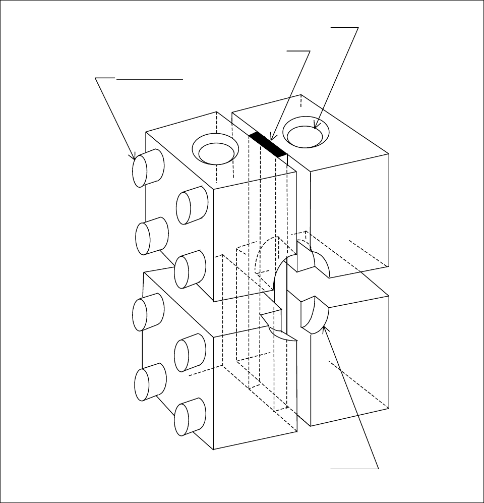
MIL-HDBK-17-1F

Volume 1, Chapter 6 Lamina, Laminate, and Special Form Characterization

6-108

the fixture will accommodate a specimen of any practical thickness. Specimens that are too thin will

buckle. Thick specimens will end-crush if the orthotropy ratio of the material being tested is too high (a

high enough shear component of the combined loading cannot be attained).

Clamping Screws

Recess

for Extensometer

Alignment Rods and Linear

Bearings

Untabbed Specimen

FIGURE 6.8.3.2.2 Schematic of ASTM D 6484 test fixture with an untabbed specimen installed.

As for ASTM D 3410, tabbed specimens, even unidirectional composites, can be tested. There is a

slight advantage of using combined loading rather than shear loading of tabbed specimens in that the

clamping forces do not have to be as high and thus the stress concentrations previously noted are not as

high.

MIL-HDBK-17-1F

Volume 1, Chapter 6 Lamina, Laminate, and Special Form Characterization

6-109

Material Forms - most specially orthotropic laminate configurations can be tested using untabbed speci-

mens. Exceptions are laminates with high percentages of 0° plies. Testing laminates with more than 50

percent 0° plies may induce end crushing. Untabbed fabric and braided composites can also be tested.

Highly orthotropic unidirectional composite specimens must be tested with tabs.

Test Fixture Characteristics - The test method relies on a high effective coefficient of friction at the

specimen-fixture interface, to transmit a significant shear force while keeping the clamping force to a

minimum. Thermal-sprayed tungsten carbide particle grip surfaces perform well. Each pair of fixture end

blocks must be properly machined and well matched at their outer ends so that when clamped on to the

specimen ends they form flat planes perpendicular to the axis of the test specimen. The specimens must

also be prepared with flat ends perpendicular to the specimen axis. A specimen is installed in the fixture

such that each end of the specimen is flush with the outer ends of a pair of clamping blocks. Then when

a compressive force is applied via flat platens, this force is transmitted both by the fixture end blocks and

the specimen ends.

Strain Measuring Devices - A typical Combined Loading Compression test fixture is provided with a re-

cess on one side so that a compressometer can be attached to one edge of the specimen in the gage

section (Figure 6.8.3.2.2). However, as in ASTM D 3410, the unsupported section is typically only about

.50 in (12.7 mm) long, limiting the attachment space available. Attaching extensometers to each face of

the test specimen, as recommended to monitor specimen bending and buckling under load, is even more

difficult because of the long reach length required. Thus, strain gages are commonly used instead.

These can have a very short active gage section length and thus fit into a confined space. Back-to-back

gages are required for a minimum number of specimens, to check for specimen bending and buckling.

Limitations of ASTM D 6484

Specimen Dimensions - The standard fixture is designed to grip each end of the untabbed specimen

over a length of 2.5 in. (63.5 mm). Thus the specimen must be longer than 5.0 in. (127 mm) in order

to establish a gage section. The maximum specimen width the standard fixture will accommodate is

1.2 in. (30.5 mm). As specimen thickness is increased, the through-thickness distribution of the axial

compressive stress will become more nonuniform. This may dictate a practical upper limit even

though the fixture can accommodate thicker specimens.

Material Forms - Highly orthotropic composite materials cannot be tested using untabbed speci-

mens. The very high clamping forces required to prevent end crushing induce stress concentrations

of unacceptable magnitudes at the gage section ends of the clamping blocks.

6.8.3.2.3 ASTM D 5467, Compressive Properties of Unidirectional Polymer Matrix Composites Using a

Sandwich Beam

The sandwich beam method (Reference 6.8.3.1(b)) consists of a honeycomb-core sandwich beam

that is loaded in four-point bending, placing the upper face sheet in compression (Figure 6.8.3.2.3). The

compression face sheet (upper sheet) is a 6-ply unidirectional laminate and the lower face sheet should

be the same material and twice as thick. The two face sheets are separated by, and bonded to, a deep

aluminum honeycomb core. The upper face sheet is designed to fail in compression when the beam is

subjected to four-point bending. The beam is loaded to failure in bending, resulting in the measurement

of compressive strength, compressive modulus and strain-at-failure if strain gages or compressometers

are employed.

Limitations of ASTM D 5467

Material Form - This test procedure is limited to unidirectional materials.

Specimen Complexity - The sandwich beam specimen is much larger, and specimen preparation is

more complex and expensive, than for those in ASTM D 3410 and ASTM D 6484.

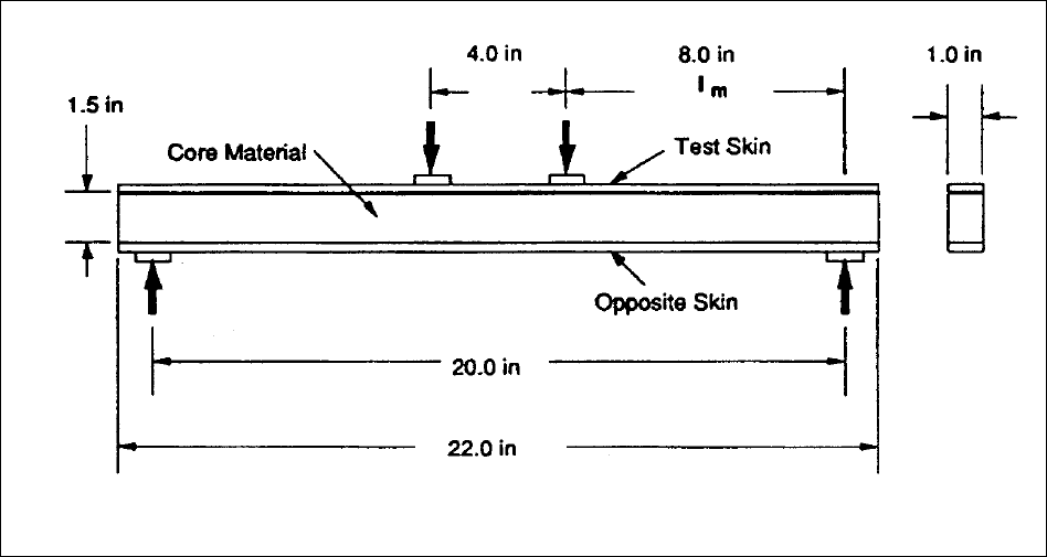
MIL-HDBK-17-1F

Volume 1, Chapter 6 Lamina, Laminate, and Special Form Characterization

6-110

Poisson's Ratio - The validity of Poisson's ratio obtained from this method has been questioned due

to anticlastic bending.

FIGURE 6.8.3.2.3 Schematic of ASTM D 5467 specimen and loading configuration.

6.8.3.2.4 ASTM C 393, Flexural Properties of Flat Sandwich Constructions

This test method (Reference 6.8.3.2.4) is one of a series designed to test sandwich constructions,

and covers the determination of the properties of flat, sandwich constructions subjected to flatwise flexure

in the same manner as ASTM D 5467. While D 5467 is designed to provide data for the compressively

loaded face sheet only, ASTM C 393 is used to determine the flexural and shear stiffness of the entire

sandwich, shear modulus and shear strength of the core, or compressive or tensile strength of the face

sheets. There are no limitations on the core or skin materials for this test method, the specimen is rec-

tangular in cross section, and the core, face, and span geometries are determined to achieve the desired

failure mode as a function of material properties. While not widely used for the determination of compos-

ite material properties, this test method does allow for the design of a test specimen not covered by

ASTM D 5467. Caution should be exercised in using this test for composite material properties since the

equations for determining the material properties may not be applicable for some specimen geometries or

core/face sheet combinations.

The use of this test method to determine the tensile properties of [90°] laminates is covered in Vol-

ume 1, Section 6.8.2.2.5.

Limitations of ASTM C 393

Material Form - This test method is not limited in the material form of the core material or face sheet

material. Equations for determining the material properties may not be applicable for some specimen

geometries or core/face sheet combinations.

Specimen Geometry - This test method is limited to rectangular sandwich construction and the core,

face, and span geometries are allowed to vary in order to achieve the desired failure mode as a func-

tion of material properties. Equations for determining the material properties may not be applicable

for some specimen geometries or core/face sheet combinations.

MIL-HDBK-17-1F

Volume 1, Chapter 6 Lamina, Laminate, and Special Form Characterization

6-111

6.8.3.2.5 ASTM D 695, Compressive Properties of Rigid Plastics

This method was developed by ASTM Committee D-20 for compression testing of unreinforced and

reinforced rigid plastics. Two types of specimens can be used for this method. The first is typically used

for unreinforced plastics and is in the form of a right cylinder or prism whose length is twice its principal

diameter or width. Preferred specimen sizes are 0.50 in. by 0.50 in. by 1 in. (12.7 mm by 12.7 mm by

25.4 mm) for a prism and 0.50 in. dia. by 1 in. (12.7 mm dia. by 25.4 mm) for a cylinder. Smaller diameter

rods or tubes may also be tested provided they are of sufficient length to allow a specimen slenderness

ratio of 11:1 to 16:1. The specimen is tested by placing it between the hardened steel faces of a com-

pressive subpress and loading it to failure.

The second test specimen configuration in the standard is documented as being for "reinforced plas-

tics, including high-strength composites and highly orthotropic laminates" < 0.125 in. (6.4 mm) thick. It

uses a flat, untabbed dogboned specimen 3.13 in. (79.5 mm) long having a 0.50 in. (12.7 mm) reduced

width test section. Two I-shaped (anti-buckling) support plates, slightly shorter than the specimen, and

with longitudinal grooves, are lightly clamped to the faces of the specimen, at most a negligible portion of

the applied force is transmitted through the support plates (a redundant load path). After positioning the

specimen between the support plates, a compressive load is applied directly to the ends of the specimen

until failure, to determine compression strength.

FIGURE 6.8.3.2.5 Schematic of ASTM D 695 specimen and test fixture.

The flat dogboned specimen, fixture-supported method was evaluated in a D-30 round robin for [0]

AS/3501 and [0] E-Glass/1002 laminates (Reference 6.8.3.2(b)). The conclusion from this study was that

this test method is not adequate for determining the compressive strength of high-modulus composite

materials in the forms studied in this investigation. (Other forms, such as E-glass fabric-reinforced com-

MIL-HDBK-17-1F

Volume 1, Chapter 6 Lamina, Laminate, and Special Form Characterization

6-112

posites, can be successfully tested using this test method.) In an attempt to modify this portion of the

ASTM D 695 test method for use with high-modulus composites, a straight-sided, tabbed coupon has

been developed. In addition, an L-shaped base to support the fixture-specimen assembly has also been

added to the test method. These modifications were not made by ASTM, nor incorporated into ASTM D

695. A discussion of these modifications is included below in the section on the SACMA SRM 1R test

method.

Limitations of the ASTM D 695 Compressive Test Method

Material Form - The published scope of this document states that it is limited to unreinforced and rein-

forced rigid plastics, including high-modulus composites. But round-robin testing conducted by ASTM

Committee D-30 found this method to be unacceptable for the measurement of strength of high modulus

composites (Reference 6.8.3.2(b)). However, it should be noted that there was some question as to the

validity of the round-robin testing (Reference 6.8.3.2(b)).

6.8.3.2.6 SACMA SRM 1R, Compressive Properties of Oriented Fiber-Resin Composites

A variation of the ASTM D 695 "Standard Test Method for Compressive Properties of Rigid Plastics"

for high-modulus continuous fiber composites has been developed and documented by SACMA as SRM

1R (Reference 6.8.3.1(d)). While essentially retaining the simple fixturing of the D 695 method, the varia-

tion utilizes straight-sided tabbed specimens for compression strength and an L-shaped base for support

of the fixture-specimen assembly. A separate, untabbed specimen must be used for the measurement of

modulus. Both specimens are shorter than the D 3410 specimens, being 3.18 in. (80 mm) long, 0.5 in.

(6.4 mm) wide and 0.040 to 0.120 in. (1 to 3 mm) thick. Although the test section is unsupported, it is

very short (0.188 in. (4.8 mm)).

This test method tends to produce slightly higher average values of compression strength (5 to 10

percent) than ASTM D 3410 Procedures A and B. One probable reason is the slightly more uniform

stress state in the gage section produced by the end loading. However, as for ASTM D 695, a fixture-

induced redundant load path through the lateral supports can be significant if the clamping force is too

high. SRM-1R specifies that the clamping screws be torqued to 6-10 in-lb (0.7-1.0 Joules). This is dis-

cussed further in (Reference 6.8.3.1(l)). A schematic of this test method with the compressive strength

specimen in place is shown in Figure 6.8.3.2.6.

Limitations of the SACMA SRM 1R Compressive Test Method

General - Separate strength and modulus specimens are required for this test method. The short

specimen gage length results in a small test section volume for the strength specimen.

Material Form - The specific scope of this test method is interpreted by the Handbook coordination

group to be for 0° direction properties of unidirectional specimens, and 0° and 0° direction properties

of fabric specimens only. This test method is applicable to fabric-based materials only when the unit

cell size of the specimen weave/braid is smaller than the 0.188 inch (4.8 mm) gage length of the

specimen.

Compressive Strength - Measured compressive strengths obtained using this test method are typi-

cally higher than those obtained using the methods in ASTM D 3410, as previously discussed. It is

important to avoid a redundant load path induced by using clamping screw torques that are too high.

Strain-at-failure - This test method will not provide strain-at-failure since the gage region of the

strength specimen is not large enough for a strain gage, and the (untabbed) modulus specimen ge-

ometry is not suitable for loading to failure. Consequently, stress-strain response, including monitor-

ing of specimen bending strains as commonly done to assess proper gage section loading, cannot be

observed over most of the actual stress-strain response.

MIL-HDBK-17-1F

Volume 1, Chapter 6 Lamina, Laminate, and Special Form Characterization

6-113

FIGURE 6.8.3.2.6 Schematic of SACMA SRM 1-88 test fixture and specimen.

6.8.3.2.7 SACMA SRM 6, Compressive Properties of Oriented Cross-Plied Fiber-Resin Composites

This test method (Reference 6.8.3.1(e)) is identical to SACMA SRM 1R with the exception that it is

limited in material form to cross-plied laminates. This limitation is applied since the method is intended for

the determination of unidirectional composite compressive strength by applying a back-out factor to the

strength determined from the cross-plied laminate.

The procedure is to test a [90/0]

(e.g., n=3 or 6) laminate

to failure in compressive as outlined in

this method (which is the same as in SACMA SRM 1R). The compressive strength of this laminate is then

multiplied by a factor to determine the effective strength of the unidirectional plies that make up the

[90/0]

laminate, as follows:

c,uni c,lam

= F

F =

σσ

where

The moduli (E

and E

) of the unidirectional composite material must be determined by separate

tests of a unidirectional composite material. A more complete discussion of the limitations and assump-

tions associated with the use of cross-ply laminate data to back out unidirectional composite data is pre-

sented in Section 2.4.2. The strength back-out factor in SACMA SRM 6 is an approximation and is not

the same as the factors recommended in Section 2.4.2.

For example, for a carbon/epoxy composite, n = 3 is typically used for the laminate lay-up when a prepreg material with an areal

weight greater than or equal to 100 g/m

is tested, and n=6 for areal weights less than 100 g/m

MIL-HDBK-17-1F

Volume 1, Chapter 6 Lamina, Laminate, and Special Form Characterization

6-114

Limitations of the SACMA SRM 6 Compressive Test Method

General - Separate strength and modulus specimens are required for this test method. The short

specimen gage length results in a small test section volume for the strength specimen. The use of

the back-out factor in this test method assumes linear elastic response of the material it is being ap-

plied to.

Material Form - Limited to cross-plied, polymer matrix composites reinforced with oriented, continu-

ous fibers, and made primarily of prepreg or similar product forms. The short gage length prohibits its

use for fabric-based and braided materials when the unit cell size of the specimen weave/braid is lar-

ger than the 0.188 in. (4.8 mm) gage length.

Compressive Strength - As for ASTM D 595 and SACMA SRM 1R, a fixture-induced redundant load

path through the lateral supports can be significant if the clamping force is too high. As for SRM-1R,

SRM 6 specifies that the clamping screws be torqued to 6-10 in-lb. (0l7-1.0 Joules). This is dis-

cussed further in (Reference 6.8.3.1(l)).

Strain-at-failure - This test method does not provide strain-at-failure since the gage region of the

strength specimen is not long enough for a strain gage, and the (untabbed) modulus specimen ge-

ometry is not suitable for loading to failure. Consequently, stress-strain response, including monitor-

ing of specimen bending strains, as is commonly done to assess proper gage section loading, cannot

be observed over most of the actual stress-strain response.

6.8.3.2.8 Through-thickness compression tests

Due to an historical lack of need for through-thickness compressive data, there are no standardized

or widely accepted test methods to determine the through-thickness (

z-direction) compressive strength,

modulus or Poisson's ratio of composite laminates. These data have been reported to a limited extent in

the literature (References 6.8.3.2.8(a) and (b)), and simple rectilinear specimens cut from thick-section

laminates have been used to obtain these properties.

6.8.3.3 Compressive test methods for developing MIL-HDBK-17 data submittal

Data provided by the following test methods (Table 6.8.3.3) are currently being accepted by MIL-

HDBK-17 for consideration for inclusion in Volume 2.

MIL-HDBK-17-1F

Volume 1, Chapter 6 Lamina, Laminate, and Special Form Characterization

6-115

TABLE 6.8.3.3 Compressive test methods for MIL-HDBK-17 data submittal.

Symbol Fully Approved, Interim

and Screening Data

Screening

Data Only

Lamina Properties

0° In-Plane Strength

D 3410, D 6484, D 5467,

SRM 1R

1,2

, SRM 6

1,2

---

0° In-Plane Modulus,

Poisson’s Ratio

D 3410, D 5467

, SRM 1R

---

90° In-plane Strength

D 3410, D 6484, SRM 1R

1,2,4

---

90° In-Plane Modulus,

Poisson’s Ratio

D 3410, D 6484, D 5467

SRM 1R

2,4

---

Out-of-Plane Strength

no recommendation ---

Out-of-Plane Modulus,

Poisson’s Ratio

, ,

νν

no recommendation ---

Laminate Properties

x In-Plane Strength

D 3410, D 6484 ---

y In-Plane Strength

D 3410, D 6484 ---

x In-Plane Modulus,

Poisson’s Ratio

D 3410, D 6484 ---

y In-Plane Modulus,

Poisson’s Ratio

D 3410, D 6484 ---

Out-of-Plane Strength

no recommendation ---

Out-of-Plane Modulus,

Poisson’s Ratio

, ,

νν

no recommendation ---

Not approved for

nor

Not approved for fabric-based materials when the unit cell size of the specimen weave/braid is lar-

ger than the 0.188 inch (4.8 mm) gage length.

Not approved for

nor

Approved for fill direction properties in cross-plied fabric based specimens only.

MIL-HDBK-17-1F

Volume 1, Chapter 6 Lamina, Laminate, and Special Form Characterization

6-116

6.8.4 Shear properties

6.8.4.1 Overview

In-Plane Shear Properties:

1,2

, F

, γ

, F

, γ

Out-of-Plane Shear Properties:

, F

, γ

, F

, γ

, F

, γ

, F

, γ

Short-Beam Strength Properties:

sbs

, F

sbs

Shear testing of composite materials has proven to be one of the most difficult areas of mechanical

property testing in which to define a rigorously correct test, especially in the out-of-plane direction. A

number of test methods have been devised, only some of which are described herein. Many of these

methods were originally developed for materials other than continuous fiber reinforced composites, such

as metal, plastic, wood, or adhesive. Several of the methods are not yet fully standardized for composite

materials, and none of the methods is without deficiency or limitation, though some are clearly more de-

sirable than others.

While there is general agreement regarding the accuracy of shear modulus measurements (for prop-

erly conducted tests), the biggest difficulty with shear testing of composites is determination of shear

strength. The presence of edge effects, material coupling effects, nonlinear behavior of the matrix or the

fiber/matrix interface, imperfect stress distributions, or the presence of normal stresses make shear

strength determination from existing shear test methods highly questionable; depending on the test, re-

sults may under- or over-estimate shear strength. Due to this uncertainty, shear strength data to be used

structural applications should be reviewed on a case-by-case basis for each given application.

A growing body of experience with composite shear testing, both published and unpublished, has led

to a greater understanding of the strengths and weaknesses of each test method. At the Fall 1991 ASTM

Committee D30 meetings, discussions in the D30.04.03 Section on Shear Test Methods led to the first

two of the following conclusions. During the Spring 1993 meetings, this group added the third conclusion.

These philosophies are being included in existing and future ASTM standard shear test methods:

1. There are no known standard (or non-standard) test methods that are capable of producing a per-

fectly pure shear stress condition to failure for every material system, although some test meth-

ods can come acceptably close on specific material systems, as judged by the end-user for a

given engineering purpose.

2. The strengths resulting from test methods that do not consistently produce a reasonable ap-

proximation of pure shear, or that do not fail via a shear failure mode, should not be termed

“shear strength.”

3. Since ultimate strength values from existing shear tests are no longer believed able to provide an

adequate criterion for comparison of material systems, the addition of an offset strength is now

recommended (0.2% offset, unless otherwise specified).

Note that shear properties generally assume subscript independence, where, for example, F

, etc. For common engineering

materials in the principal material coordinate system, this is a commonly accepted and generally accurate assumption. However, in

unbalanced, multi-directional laminates, the shear stiffness, shear strength, or both, can be direction dependent. In such laminates

this arises primarily from the difference in behavior between tension and compression of the fibers that are oriented off-axis relative

to the loading direction.

Transverse isotropy, a common assumption for many material systems, implies that G

MIL-HDBK-17-1F

Volume 1, Chapter 6 Lamina, Laminate, and Special Form Characterization

6-117

With the highly nonlinear stress-strain behavior of many filamentary composites, and especially with

high-elongation material systems, it is common to terminate a shear test prior to actual specimen failure.

Following the lead of MIL-HDBK-17, ASTM D30 currently recommends ending shear testing at 5% shear

strain, if failure has not previously occurred. The rationale for this is included in the following discussions.

Practical usage in structural laminates---Typical structural laminates are designed to have fibers aligned

with major load-carrying directions. In the case of shear, the shear loads are usually carried in fi-

ber tension or compression by plies oriented at the appropriate angle. Since, from basic mechan-

ics of materials, the shear strain in the matrix of a given ply cannot be more than twice the fiber

axial strain of another ply oriented at 45

° to the first ply, we can see that an upper bound on the

useful engineering value of shear strain is twice the tensile or compressive fiber strain. As the

most ductile structural fibers currently fail well below 2.5%, a practical upper limit for shear strain

in a structural laminate would be 5%. Terminating shear test data at this shear strain value is a

practical recommendation that saves time in testing and yields a more structurally attainable, and

therefore more meaningful, lower-bound estimate of ultimate shear strength.

Limitations of common shear test methods---There are kinematic limitations with both the

±45° tensile

shear test and the V-notched beam (Iosipescu) shear test, due to excessive scissoring of the fi-

bers. The work of Kellas et al (Reference 6.8.4.1) showed that the initial condition of

±45° ply ge-

ometry changes significantly at high shear strains. Based on their estimate of the relationship be-

tween fiber scissoring and shear strain, the test results for these tests become questionable past

5% shear strain, which then becomes a practical upper strain limit for these test methods.

A different issue that results in a similar restriction involves the use of typical strain gages. If gages are

used for strain measurement, as is feasible with some tests and required by others, the typical

gage limit of about 3% extensional strain equates to roughly 6% shear strain, making this a prac-

tical limit for shear strain measurement that is similar in value to the kinematic restriction.

Laminate Testing --- Certain shear test methods, like the

±45° tensile shear test, are by their very nature

capable of testing only certain types of laminates. And, as difficult as determination of ultimate

material shear strength is for current shear test methods, shear strength of a multi-directional

laminate is even more problematic. While several of the shear test methods discussed herein are

capable of determining a substantial portion of a laminate stress-strain curve and with it a shear

modulus, there is no standard test method that has been shown to adequately determine the ul-

timate shear strength of a multi-directional laminate. A modification of ASTM D4255 (rail shear

test method) using bonded, tapered, tabs have been suggested for shear strength testing of

multi-directional laminates, but interest to date has not been sufficient to either standardize this

modification or allow MIL-HDBK-17 to recommend it for widespread use. MIL-HDBK-17 Testing

Working Group will continue to follow developments in this area.

6.8.4.2 In-plane shear tests

6.8.4.2.1 ±45° tensile shear tests

1) ASTM D 3518/D 3518M-94, Test Method for In-Plane Shear Response of Polymer Matrix Composites

by Tensile Test of a

±45° Laminate

2) SACMA SRM 7R-94, In-plane Shear Stress-Strain Properties of Oriented Fiber-Resin Composites.

This test (References 6.8.4.2.1(a) and (b)) for in-plane shear properties consists of a modified ASTM

Test Method D3039 tensile test of a specimen having a ply lay-up of the [

±45]ns family. Away from the

gripping region the in-plane shear stress in this specimen can be shown to be a simple function of the

average applied tensile stress, allowing for straightforward calculation of the shear response of the mate-

rial. This test method has the advantages of a simple test specimen, requires no fixturing, and measure-

ment of strain can be performed using either extensometers or strain gages.

MIL-HDBK-17-1F

Volume 1, Chapter 6 Lamina, Laminate, and Special Form Characterization

6-118

Originally applied only to unidirectional materials, the 1994 release of the standard now includes

many woven fabric materials, but the test method is inherently restricted to determination of properties in

the 1-2 material plane. The SACMA version has historically been a restricted subset of the ASTM stan-

dard; though there have been minor differences between current releases of the two methods in the past.

However, the versions listed herein have several significant differences. The 1994 SACMA test method

does not include several significant changes that were made to D 3518 in 1994, and though the basic

physics of the test remain identical, the details of data reduction are now distinctly different so the two

version are not fully equivalent. D 3518 now defines the chord modulus from 2000 to 6000 shear mi-

crostrain (versus 500-3000 in SRM 7R-94), and terminates the test at 5% shear strain (or failure, which-

ever comes first), while SRM 7R-94 still defines strength based only on ultimate load. D 3518 also has

added an offset strength, which SRM 7R-94 does not include.

Good modulus agreement has been shown between the

±45° test method and other shear test meth-

ods (References 6.8.4.2.1(c) through (e)), although the stress-strain response has been shown to be un-

derestimated at shear strain levels above 1.3% (Reference 6.8.4.2.1(f)). There is a feeling by many in the

aerospace composite structures community that while the stress state of this specimen may not be “pure,”

it does respond in a manner that mimics the actual stress state and ply interaction within a structural

laminate. The resulting response yields an “effective” shear modulus that may be preferred by the de-

signer.

Previous versions of the ASTM standard lacked sufficient definition of several test parameters that

have since been found to have significant effects on the ultimate strength of this specimen. It has been

shown (Reference 6.8.4.1) that this specimen does not fail due to in-plane shear, but rather due to com-

plicated interactions that are sensitive to material toughness, ply stacking sequence, ply count, ply thick-

ness, edge effects, and surface ply constraints. The 1994 release of D 3518 provides additional controls

that improve this situation:

• “Ultimate shear strength” has been replaced with “shear stress at 5% shear strain”, since it is now

agreed that this test cannot determine a true ultimate material strength. This new quantity is analo-

gous to the old ultimate strength value, but since it is calculated differently, for many material systems

they will not be exact equivalents, and may be significantly different.

• Adds an offset shear strength (a more meaningful quantity for material comparison than the previous

“ultimate” shear strength).

• Terminates the test at 5% shear strain, if the specimen has not already failed by rupture.

• Changes the chord shear modulus to use a strain range (2000-6000 shear microstrain) that is con-

sistent with the tensile chord modulus strain range (1000-3000 microstrain).

• Provides requirements for ply lay-up that assure that the most brittle modes of failure will be avoided,

and increase the likelihood that data comparisons will be more meaningful.

Refer to the references, or to the discussion within the ASTM standard itself, for more details.

Limitations of the

±45° tensile shear test:

Material and Laminate Form---Limited to materials available in a fully balanced and symmetric

±45°

specimen. As discussed above, the stacking sequence, ply count, and ply thickness have a di-

rect effect on specimen strength. Low ply count laminates and repeating (or very thick) plies

have a deleterious effect on strength and are restricted in the new standard.

Inhomogeneous Materials---The material is assumed homogenous with respect to the size of the test sec-

tion. Material forms with features that are relatively coarse with respect to the test section width,

such as woven or braided textiles with a coarse repeating pattern, require a larger, currently non-

standard, specimen width.

Impurity of Stress State---The material in the gage section is not in a state of pure in-plane shear, as an

in-plane normal stress component is present throughout the gage section, and a complex stress

MIL-HDBK-17-1F

Volume 1, Chapter 6 Lamina, Laminate, and Special Form Characterization

6-119

field exists near the free edges. Although the specimen is believed to provide reliable initial mate-

rial response, and can establish shear stress-strain response well into the nonlinear region, the

calculated shear stress at failure does not represent the material strength, which is why the ASTM

standard now terminates the test at 5% shear strain.

Effects of Large Deformation---The extreme fiber scissoring that can occur in this specimen in ductile

specimens changes the fiber orientation progressively with increasing strain, conflicting with the

fiber orientation assumptions used in the calculation of results. This is a second reason why the

test is now terminated 5% shear strain.

6.8.4.2.2 Iosipescu shear test

ASTM D 5379/D 5379-93, Test Method for Shear Properties of Composite Materials by the V-Notched

Beam Method.

The V-notched beam shear test (often called the Iosipescu test in the literature) has been standard-

ized for composites by ASTM Committee D-30 in ASTM D 5379/D 5379M-93 (Reference 6.8.4.2.2(a)).

The concept for the v-notched beam shear test for strength and modulus was originally identified in the

late 1950's and early 1960's by Arcan (References 6.8.4.2.2(b) through 6.8.4.2.2(d)) and Iosipescu (Ref-

erence 6.8.4.2.2(e) through 6.8.4.2.2(g)) for use on metals. Subsequent usage was limited until detailed

investigations were begun on an improved specimen and fixture at the University of Wyoming under

NASA funding during the early 1980's (References 6.8.4.2.2(h) and (i)). The fixture was subsequently

modified (References 6.8.4.2.2(j) and (k)), and this latter Wyoming configuration formed the basis for the

ASTM standard. This method has been investigated extensively; see References 6.8.4.2.2(l) through

6.8.4.2.2(r)) for additional investigations. Early historical perspectives are given in References

6.8.4.2.2(h) and 6.8.4.2.2(s). However, the remainder of the discussion focuses on the configuration that

has been standardized.

In this method, a material specimen in the form of a rectangular flat strip with symmetrical centrally

located v-notches, shown schematically in Figure 6.8.4.2.2(a), is loaded in a mechanical testing machine

by a special fixture, shown schematically in Figure 6.8.4.2.2(b). Either in-plane or out-of-plane shear

properties may be evaluated, depending upon the orientation of the material coordinate system relative to

the loading axis.

While the standard only addresses determination of properties in the material coordinate system, the

initial stress-strain response of general multi-directional laminates may also be determined. However the

method of load introduction into the specimen is generally not capable of reacting the much higher loads

sustainable by a multi-directional laminate, and therefore for most material systems this test method is

limited, for multi-directional laminates, to characterization of elastic modulus and the initial portion of the

stress-strain curve. A few multi-directional materials have been successfully tested, such as the discon-

tinuously reinforced, multi-directional, molded material commonly called sheet-molding compound (SMC),

but such materials remain the exception rather than the rule.

The specimen is inserted into the fixture with the notch located along the line-of-action of loading via

an alignment tool that centers the specimen in the fixture. The upper head of the fixture is attached to

and driven downward by the cross-head of the testing machine, while monitoring load. The relative dis-

placement between the two fixture halves loads the notched specimen. By placing two strain gage ele-

ments, oriented at

±45° to the loading axis, in the middle of the specimen (away from the notches) and

along the loading axis, the shear response of the material can be measured.

The object of the VNB concept can be seen in the idealization of the applied loading as asymmetric

flexure, shown in the shear and bending moment diagram of Figure 6.8.4.2.2(c). The specimen gage

area is in the region of constant shear and zero moment. The specimen notches influence the shear

strain along the loading direction, making the shear distribution more uniform than would be seen without

MIL-HDBK-17-1F

Volume 1, Chapter 6 Lamina, Laminate, and Special Form Characterization

6-120

the notches.

The degree of uniformity in the shear distribution is a function of material orthotropy; the

best overall in-plane shear results have been obtained on [0/90]ns-type laminates. However, while the

point-loading idealization indicates constant shear loading and zero bending moment in the gage section

of the specimen, in practice the fixture applies distributed loads to the specimen that contribute to an

asymmetry in the shear strain distribution and to a component of normal stress which is particularly dele-

terious to [90]n specimens.

FIGURE 6.8.4.2.2(a) V-notched beam test coupon schematic.

Limitations of the v-notched beam shear test:

Inhomogeneous Materials--- The material is assumed homogeneous with respect to the size of the test

section. Materials that have relatively coarse features with respect to the test section dimensions, such

as fabrics using large filament count tows (such as tows of 12000 filaments or more) or certain braided

structures, should not be tested with this specimen size.

Uniformity of Strain Field--- The calculations assume a uniform shear strain state between the notches.

The actual degree of uniformity varies with the level of material orthotropy and the direction of loading. A

new strain gage grid configuration has recently been developed specially for use with this test method.

The active grid on this gage extends from notch-to-notch and provides an improved estimation of the av-

erage strain response. When using conventional strain gages the most accurate measurements of in-

plane shear modulus for unidirectional materials have been shown to result from the [0/90]ns specimen.

An isotropic beam in shear has a parabolic shear stress profile.

MIL-HDBK-17-1F

Volume 1, Chapter 6 Lamina, Laminate, and Special Form Characterization

6-121

Load Eccentricity--- Twisting of the specimen during loading can occur, affecting strength results, and es-

pecially, elastic modulus measurement. It is recommended that at least one specimen of each sample be

tested with back-to-back rosettes to evaluate the degree of twist.

Determination of Failure--- Failure is not always obvious in certain materials or configurations. See the

standard test method (Reference 6.8.4.2.2(a)) for more information.

Instrumentation: Strain gages are required.

FIGURE 6.8.4.2.2(b) V-notched beam test fixture schematic.

MIL-HDBK-17-1F

Volume 1, Chapter 6 Lamina, Laminate, and Special Form Characterization

6-122

FIGURE 6.8.4.2.2(c) Idealized force, shear, and moment diagram.

MIL-HDBK-17-1F

Volume 1, Chapter 6 Lamina, Laminate, and Special Form Characterization

6-123

6.8.4.2.3 Rail shear tests

ASTM D 4255-83, Guide for Testing for In-plane Shear Properties of Composite Laminates.

In 1983, ASTM Committee D-30 published D 4255 (Reference 6.8.4.2.3(a), a standard covering in-

plane shear properties of composite laminates by either of two rail shear methods. The round-robin test-

ing conducted by D-30 to understand the precision and bias of these methods found, at the time, a large

amount of variability in results between laboratories. While the sources of this variability were not well

understood at the time, a standard for this test method was strongly desired since rail shear tests were in

wide use. The standard was completed and released, though with caveats, in order to provide a common

ground for the users.

Since the initial release of D 4255, several testing factors that could have contributed to the scatter in

the initial round-robin data have become better understood, and a revision to this standard is in progress

at this writing (1997) that will correct several obvious shortcomings in the initial release. Whether the re-

vised standard will have improved/reduced variability and gain the confidence of new users, particularly in

the face of the substantial research that has since improved competing simpler and less expensive test

methods, remains to be seen.

While the standard is restricted to in-plane testing, it is capable of testing for either material shear or

multi-directional laminate shear properties. However the current version of the standard is limited, as is

the D 5379 Iosipescu shear test, to characterization of modulus or initial shear stress-strain response,

since the standard means of applying load to the specimen generally cannot sustain the higher strengths

of multi-directional laminates. Development of standard rules for application of bonded, tapered tabs to

multi-directional laminates is needed, since this approach is one of the most promising for shear strength

determination of off-axis configurations. However, more work remains to be done before a bonded, ta-

pered, tab modification to D 4255 can be standardized or recommended by MIL-HDBK-17.

As the shear stress state is not uniform through the specimen, and as failures are often noted to be-

gin outside the center of gage section (such as at the restrained corners of the plate) this test as currently

standardized does not always produce reliable shear strength data (Reference 6.8.4.2.3(b)). The three-

rail test has a purer state of stress (Reference 6.8.4.2.3(c)), although it requires a larger specimen size of

approximately 150 mm by 150 mm (6 in. by 6 in.)

Limitations of the D 4255-83 rail shear tests:

Specimen Size: Both version require larger specimens than other shear tests.

Instrumentation: Strain gages are required.

Stress State: The stress state is known to be non-uniform, and the failure mode is typically influenced by

non-shear failures starting outside of the gage section.

Data Scatter: High data scatter from round-robin tests cast doubt upon the ability of these methods to

produce repeatable data, at least in their current form.

6.8.4.2.4 Ten-degree off-axis shear test

This method, first reported by Chamis and Sinclair (Reference 6.8.4.2.4) uses a straight-sided, rec-

tangular unidirectional tensile specimen with the fiber oriented at ten degrees to the loading direction

(Figure 6.8.4.2.4). Note that the material specimen is limited to unidirectional filamentary laminates. This

specimen, like the ASTM D 3518 specimen above, is also not under a state of pure shear and suffers

from the effects of a combined stress state. This test produces results of generally higher modulus and

significantly lower strengths than the other shear test methods such as ASTM Test Methods D 3518 or D

MIL-HDBK-17-1F

Volume 1, Chapter 6 Lamina, Laminate, and Special Form Characterization

6-124

5379. This test method is inherently restricted to evaluation of the shear response in the 1-2 plane, and is

therefore not applicable to shear evaluation of laminates.

Limitations of the 10° off-axis shear test:

Material Form: Limited to unidirectional laminates.

Stress State: Known to have a significantly biased stress state producing an overly stiff initial response

and premature failure.

Lack of Standardization: Has never been standardized.

FIGURE 6.8.4.2.4 Ten-degree off-axis tension shear test.

6.8.4.2.5 Tube torsion tests

1. ASTM E143-87, Test Method for Shear Modulus at Room Temperature

2. MIL-STD-375, Test Method for In-Plane Shear Properties of Hoop Wound Polymer Matrix Composite

Cylinders

3. ASTM D 5448/D 5448M-93, Test Method for In-Plane Shear Properties of Hoop Wound Polymer Ma-

trix Composite Cylinders

Torsion testing of tubes has been standardized by ASTM since 1959 by Test Method E143-87 (Refer-

ence 6.8.4.2.5(a)). While broad in scope, and technically not exclusive of composites, Test Method E143

was primarily developed for metals. However the concept has also been applied to composites, where the

challenge becomes in applying load to the specimen without producing a grip-induced failure; a typical

gripping arrangement is shown in Figure 6.8.4.2.5. A torsion test specifically for wound composite tubes

was developed and released as Military Standard, MIL-STD-375 (Reference 6.8.4.2.5(b)). MIL-STD-375

was submitted to ASTM for non-military standardization, and with minor changes was approved as ASTM

D 5448/D 5448M-93. Test Method D 5448 (Reference 6.8.4.2.5(c)) consists of a 100 mm (4 in.) nominal

MIL-HDBK-17-1F

Volume 1, Chapter 6 Lamina, Laminate, and Special Form Characterization

6-125

diameter hoop-wound tube, which is gripped at each end and twisted via a fixture until failure. This test

has been shown to produce good results and is the theoretical ideal for determining both in-plane shear

strength and modulus. Note that since the MIL-STD test method has since been withdrawn by the U.S.

DOD it should no longer be referenced; it has been superseded by the ASTM test method.

FIGURE 6.8.4.2.5 Typical torsion tube shear fixture (Reference 6.8.4.2.5(d)).

While not within the scope of current test standards, these tests, which are inherently restricted to in-

plane usage, can be applied to laminate testing as well as lamina testing. However, gage section speci-

men failures may be difficult to achieve in the multi-directional laminates, due to the higher loads devel-

oped in the presence of off-axis fibers. Loading point modifications will usually be required for laminate

testing.

Limitations of the torsional tube methods:

Material Form: If not using filament-wound materials the process required to create the tube may be sig-

nificantly different than that used in the structure.

Cost of Specimen Fabrication: Fabrication of the specimen can be a significant undertaking requiring un-

usual expense.

Stress Concentration: A stress concentration exists at the end grips, as noted by Guess and Haizlip (Ref-

erence 6.8.4.2.5(d)), tending to result in failures in the gripping area, unless extreme precautions are

taken.

Instrumentation: Strain gages are required.

6.8.4.3 Out-of-plane shear tests

6.8.4.3.1 Short-beam strength tests

1) ASTM D 2344-84, Test Method for Apparent Interlaminar Strength of Parallel Fiber Composites by

Short-Beam Method

MIL-HDBK-17-1F

Volume 1, Chapter 6 Lamina, Laminate, and Special Form Characterization

6-126

2) SACMA SRM 8R-94, Apparent Interlaminar Shear Strength of Oriented Fiber-Resin Composites by the

Short-Beam Method

ASTM Test Method D 2344 (Reference 6.8.4.3.1(a), commonly known as the short-beam strength

(SBS) test, attempts to quantify the interlaminar (out-of-plane) shear strength of parallel fiber reinforced

composites.

The specimen for this test is a short, relatively deep beam cut from a flat laminate. The

specimen is mounted as a simply supported beam and loaded at the midpoint of the span of the speci-

men. The intent is to minimize bending stresses while maximizing out-of-plane shear stresses by using a

short, deep “beam.”

However, the contact stresses induced at the load points greatly interfere with the strain distribution

both through the depth of the beam and axially along the length of the beam. The resulting failure is

rarely, if ever, a true pure shear failure but instead results from the complex stress state present in the

specimen, as shown by Berg et al (Reference 6.8.4.3.1(b)) and others.

Unfortunately this test has commonly been used in the past (and is still used by some) to develop

design allowables for structural design criteria. In the absence of any other choice this is understandable,

though regrettable. However, the availability of the v-notched beam method, discussed in Section

6.8.4.3.2, makes the use of the short-beam strength test for property determination obsolete.

The short beam strength test should only be used for qualitative testing such as material process de-

velopment and control. As a quality control test use of laminate configurations other than unidirectional

are common, though currently non-standard.

The ASTM standard is currently being revised and updated to allow the standard SBS testing of bal-

anced and symmetric laminates. A related method is SACMA SRM 8R-94 (Reference 6.8.4.3.1(c)).

Limitations of the short beam strength test include:

Stress State: The stress state is known to be significantly disruptive and three-dimensional. The resultant

strengths are a poor estimation of the out-of-plane shear strength.

Failure Mode: The failure mode is most often multi-mode.

No Modulus/Material Response: Instrumentation of this specimen is not practical, therefore modulus and

stress-strain data cannot be obtained.

6.8.4.3.2 Iosipescu shear test

This test method and the specimen geometry are described for in-plane shear testing in Section

6.8.4.2.2. When testing for out-of-plane shear properties the orientation of the fibers in the laminate is

changed so as to cause a shearing action in the desired transverse plane. This test method is the only

acceptable out-of-plane shear test available. The out-of-plane testing of laminates with fibers off-axis to

the test direction, such as 3-dimensional textiles, are subject to the same restrictions and limitations that

are discussed in the section on in-plane Iosipescu testing (6.8.4.2.2).

6.8.4.3.3 ASTM D 3846-79, Test Method for In-Plane Shear Strength of Reinforced Plastics

ASTM Test Method D 3846 (Reference 6.8.4.3.3), despite the title, is not normally used as an in-

plane shear strength test (using the most common definition of in-plane in the terminology of advanced

composites) but is in fact an out-of-plane shear strength test and as such is covered in this section on

out-of-plane shear tests.

A currently fully equivalent, but more restricted, subset of ASTM D2344 has been promulgated by the composite materials suppli-

ers as SRM 8R-94 (Reference 6.8.4.3.1(c)). However, it is expected that, barring a parallel revision to SRM 8R-94, the two docu-

ments will diverge as a result of the on-going revision to ASTM D2344.

MIL-HDBK-17-1F

Volume 1, Chapter 6 Lamina, Laminate, and Special Form Characterization

6-127

This test is primarily intended for use on randomly-dispersed fiber-reinforced thermosetting sheet

plastics as a substitute to the short-beam strength test, Test Method D 2344 (Reference 6.8.4.3.1(a)), de-

scribed in Section 6.8.4.3.1. The test consists of a doubly notched specimen loaded compressively in a

supporting jig (the same fixture used in the Test Method D 695 compression test). Failure occurs in out-

of-plane shear in the plane of the specimen between the two centrally located opposing square notches.

While this specimen can be (and has been) used for testing continuous-fiber laminated reinforced plas-

tics, it is not recommended for use on advanced composite laminates. The notches, which are machined

into the specimen to force failure of the laminate in shear, were found by Herakovich et al (Reference

6.8.4.2.2(n)) to negatively influence the stress distribution in the specimen. As a result, a non-uniform,

multiaxial stress state exists in the gage section, making a true strength calculation suspect at best.

Limitations of the D 3846 notched compression test:

Stress State: A highly three-dimensional, non-uniform stress state in the gage section cause strength val-

ues from this test to be unusually poor estimations of the true out-of-plane shear strength.

No Modulus/Material Response: Instrumentation of this specimen is not practical, therefore modulus and

stress-strain data cannot be obtained.

6.8.4.4 Shear test methods for MIL-HDBK-17 data submittal

Data produced by the test methods in Table 6.8.4.4 are currently being accepted by MIL-HDBK-17 for

consideration for inclusion in Volume 2.

TABLE 6.8.4.4 Shear test methods for MIL-HDBK-17 data submittal.

Property Symbols Fully Approved, In-

terim, and Screening

Data

Screening Data Only

In-Plane Shear

Strength (lamina)

D 3518

SRM 7

D 5379

D 5448

---

In-Plane Shear

Strength (laminate)

--- ---

In-Plane Shear

Modulus (lamina)

D 3518

SRM 7

D 5379

D 4255

D 5448

---

In-Plane Shear

Modulus (laminate)

D 5379

D 4255

---

Out-of-Plane Shear

Strength

so su

23 23

D 5379 ---

Out-of-Plane Shear

Modulus

xz yz

31 23

D 5379 ---

Short Beam Strength

SBS

--- D 2344

SRM 8

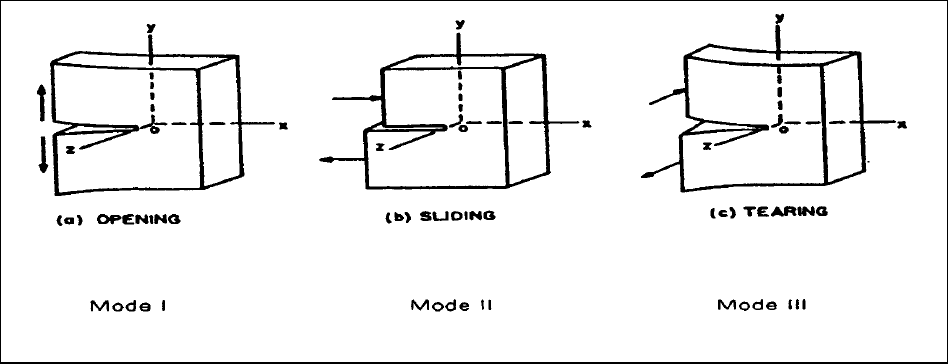
MIL-HDBK-17-1F

Volume 1, Chapter 6 Lamina, Laminate, and Special Form Characterization

6-128

6.8.5 Flexural properties

There is not a recommended test method for determining the flexural properties of composite lami-

nates. Even though there are approved flexural test methods, there is some debate as to the validity of

the results.

Within the aerospace industry, flexure testing is primarily used for quality control. ASTM Test Method

D 790, "Flexural Properties of Unreinforced and Reinforced Plastics and Electrical Insulating Materials",

was originally written for plastics but has since been modified and approved for composites (Reference

6.8.5). In some cases, ASTM Test Method C 393, "Flexure Test of Flat Sandwich Constructions", has

been adapted for use with composite laminates (Reference 6.8.2.2.5).

6.8.6 Fracture toughness properties

6.8.6.1 Overview

Fracture in structural solids, such as wood, glass, metals, rock and concrete, is usually initiated by

some crack or notch-like flaws, which cause high stresses in the neighborhood of such flaws. Inglis (Ref-

erence 6.8.6.1(a)) pointed out the significance of the localized concentration of stress near the tip of a

sharp notch. A criterion of fracture based on the first law of thermodynamics was proposed by Griffith

(Reference 6.8.6.1(b)), who postulated that the reduction in strain energy due to propagation of a crack is

used to create new crack surfaces. Strain energy release rate,

G, is defined as the reduction in strain

energy (or increase in potential energy) due to an infinitesimal self-similar extension of the crack and

catastrophic propagation of the crack will occur when this rate reaches a critical value,

. For a through

crack of length 2a in a thin or a thick plate, subjected to a tensile stress

, the energy release rate can

be expressed in terms of

, a and the properties of the material. Irwin (Reference 6.8.6.1(c)) pointed out

that in isotropic materials, three independent kinematic movements are possible, by which the upper and

lower crack surfaces can displace with respect to each other. These movements are schematically de-

picted in Figure 6.7.8.1. Only the first mode (Mode I or opening mode) was considered by Griffith. Irwin

showed that the crack tip stresses can be expressed by a three parameter set of equations. These pa-

rameters,

, K

III

, called the Mode I, Mode II and Mode III stress intensity factors, are functions of the

crack dimensions and the applied loads and critical values of these parameters govern the phenomenon

of unstable crack growth. The concept of failure based on the critical value of a stress intensity factor has

been shown to be equivalent to that proposed by Griffith in terms of the critical strain energy release rate

(

, G

IIc

, or G

IIIc

). Irwin also suggested the use of the critical value of the total energy release rate as the

parameter governing failure, provided failure occurs by self-similar crack propagation. These concepts

have also been extended to orthotropic materials (Reference 6.8.6.1(d)).

FIGURE 6.8.6.1 Basic modes of crack extension.

MIL-HDBK-17-1F

Volume 1, Chapter 6 Lamina, Laminate, and Special Form Characterization

6-129

Use of fracture mechanics has gained wide acceptance in predicting failure in metal structures (Ref-

erences 6.8.6.1(e)-(g)) and various test methods have been developed for determining

(or G

) as well

as crack growth resistance curves for cases when stable crack growth is possible. Further, over the

years, there has emerged a fracture mechanics design procedure for fatigue of metal aeronautical struc-

tures, which is based on periodic inspection for monitoring visible cracks and predicting residual life using

crack growth laws of the power law type (References 6.8.6.1(h) and (i)). Various attempts have been

made to use fracture mechanics based methods for predicting failure of thin laminates with through

cracks or notches (Reference 6.8.6.1(j)). However, it has been found that linear elastic fracture mechan-

ics treating the thin laminates as orthotropic or isotropic plates is not useful because of considerable sub-

critical surface damage near the crack tips. Semi-empirical corrections are often employed for predicting

strength of thin notched laminates (Reference 6.8.6.1(k)). On the other hand, fracture mechanics ap-

proaches appear to yield better results for thick laminates containing through cracks or deep surface flaws

(References 6.8.6.1(l) through 6.8.6.1(n)) . It has also been shown that crack growth resistance or the R-

curve concept, originally proposed for modeling stable crack growth (with increasing load) in metals, is

useful for predicting fracture in notched chopped fiber composites (Reference 6.8.6.1(o)). Although use

of fracture mechanics in the problems just described has been very limited, it is now being widely used in

the industry for dealing with various problems involving delamination fracture. Delaminations (in resin rich

regions between the plies in a laminate) can exist as manufacturing defects or can be created due to

various reasons; namely, (i) coalescence of small voids at interfaces, (ii) foreign object impact and (iii)

peculiar stress fields near discontinuities such as free edges, holes, ply drops, transverse ply cracks or

bonded joints. The basic concepts of delamination fracture are the same as those discussed earlier.

However, the strain energy release rate, which is the energy released due to infinitesimal extension (as

described earlier for through cracks in a plate) of a delamination is commonly used for prediction of catas-

trophic fracture and various test methods have been proposed for determination of its critical value (often

called the toughness) for each of the three modes of loading (I, II, and III as shown in Figure 6.8.6.1).

Some tests have also been devised for determining the criteria of failure (mode interaction) under mixed

mode conditions. The next section gives some general discussions on the test methods and use of the

properties in practical applications. Subsequent sections deal with some of the test methods.

6.8.6.2 General discussion

It should be noted that although the subject is quite advanced at this point and various attempts have

also been made to obtain (i) R curves for modeling stable delamination growth under increasing load and

(ii) delamination growth law for predicting delamination extension under cyclic loading, only one test

method has been standardized. The test specimens usually contain an implanted delamination in the

form of a nonadhesive insert and have been used widely for unidirectional glass or carbon fiber reinforced

composites. The tests are designed such that delamination growth direction coincides with the fiber di-

rection. Toughness values or other characteristics may sometimes vary depending on the tendency of the

delamination to wander around various phases of multiple phase matrix materials. Also, brittle matrix

composites with tough adhesive interleaves may yield different properties depending on the region where

the delamination propagates, i.e., interleaves, brittle matrix or the interface. Use of non-unidirectional

specimens with implanted delaminations between two off-axis plies of the same orientation or between

two plies of different orientations may cause the delamination to shift its path through ply cracks and in-

terpretation of data for such cases is difficult. It is also likely that the properties will differ if the delamina-

tion propagates in a direction other than the fiber direction, even though it remains coplanar. Woven fab-

ric composites may show more scatter as compared to that for unidirectional laminates and increasing

tendency of stable delamination growth (R-curve) because of the typical structural arrangement in such

materials.

The main reason for observed resistance to delamination growth (for stable growth commonly ob-

served in Mode I tests) in unidirectional brittle matrix composites is the phenomenon of fiber bridging

across the delamination plane. Such bridging is caused by fiber nesting that is typically present in unidi-

rectional composites and, hence, the toughness value for initiation should be identified separately from

those at later stages of delamination growth. This value should be representative of the toughness for a

natural delamination and it is often used to obtain a conservative design criterion. R-curves obtained from

tests are not commonly used to obtain generic material property data. They are, however, often used to

MIL-HDBK-17-1F

Volume 1, Chapter 6 Lamina, Laminate, and Special Form Characterization

6-130

compare the degree of fiber matrix bonding between specimens, panels or batches of the same material

or to compare composites with the same fiber, but different matrices. Poor bonding usually results in

greater fiber bridging and, hence, a greater increase in

with delamination length.

In materials not strongly influenced by fiber bridging, a competing mechanism may dominate. When

the delamination starts to grow from the insert, a pop-in type of behavior (yielding higher toughness val-

ues than that for subsequent growth) is observed. For Mode I tests, the first point is neglected in such

cases and results for subsequent growth (made possible by displacement controlled tests) are utilized.

For Mode II or mixed mode tests, failure is usually catastrophic and for this reason precracking (extension

of the delamination beyond the insert) by Mode I loading, wedge insertion, or other methods is usually

employed.

Most of the tests utilize beam type specimens with a single delamination tip. As the load is increased,

load point deflections are measured and delamination growth is observed visually or using other aids or

devices. In some cases, catastrophic delamination growth is observed (as in Mode II tests) and the

maximum load reached is noted. Otherwise (in displacement controlled tests), load-displacement plots

remain linear up to a point beyond which the delamination extends and a load drop occurs. In some ma-

terials, the onset of nonlinearity may be noticed before any delamination growth is noticeable. Such be-

havior may occur due to inelastic material response or subcritical damage growth ahead of the tip. The

measured values of loads, deflections, and delamination lengths at the point of onset of nonlinearity or

delamination growth are utilized to compute the critical energy release rates associated with fracture or

subcritical damage growth. In some cases, approximate closed form expressions of energy release rates

in terms of load, deflection, delamination length and/or material (or beam) stiffnesses are utilized for data

reduction. When the deflection can not be measured and there is some uncertainty about the stiffness,

an alternate approach is to first perform a compliance calibration on the specimen (or similar specimens)

where the compliance

C =

6.8.6.2(a)

being the deflection associated with the applied load P, for various values of delamination, length a is

fitted to an exact or approximate relation (based on the principles of mechanics or a polynomial). The

energy release rate is given by

G = -

6.8.6.2(b)

G =

6.8.6.2.(c)

where

b is the specimen width and a the delamination length. U and V are the strain and potential ener-

gies, respectively, both expressed in terms of displacements.

Now,

U =

P =

6.8.6.2.(d)

and

V = -

P = -

6.8.6.2.(e)

Therefore, it follows that for displacement controlled tests (

prescribed)

G =

6.8.6.2.(f)

It can be shown that the same relation holds for load controlled tests. This approach is not suitable for

mixed mode tests because the individual components of the energy release rates can not be calculated in

this manner, unless their contribution to the total energy release rate is known.

As discussed in the previous section, catastrophic fracture in a single mode can be predicted using

the critical strain energy release rate for the particular mode provided, of course, the energy release rate

MIL-HDBK-17-1F

Volume 1, Chapter 6 Lamina, Laminate, and Special Form Characterization

6-131

is constant along the delamination front. If these rates vary over the front, a conservative estimate can be

obtained by equating the maximum value of this quantity at a point as determined from finite element or

other stress analyses to the critical value (numerous investigations are reported in literature for such cal-

culations, but they are beyond the scope of this section). Such estimates are often adequate for design

purposes unless the delamination gets arrested because of structural or other constraints. A similar ap-

proach can be employed for estimating stable growth pattern and instability point using the R-curve con-

cept. Growth of such delaminations under cyclic loading can be estimated using experimentally deter-

mined power law type growth laws, where the maximum value (or range) of the energy release rate is the

controlling parameter. Uses of R-curves for predicting stable crack growth and power laws for estimating

growth per cycle are, however, not yet accepted in the industry, since there exists some evidence that

they do not always yield generic characterizations (Reference 6.8.6.2(a)).

The problem becomes more complicated when mixed mode conditions are present and the tough-

ness values for the three modes differ significantly from one another. Various fracture criteria have been

proposed for prediction of quasistatic fracture. A survey of such criteria for combined action of Modes I

and II can be found in Reference 6.8.6.2(b). Power law type growth laws with the maximum value (or the

range) of a scalar function f of the energy release rates (

f = G

+ G

III

is a simple example) or the

stress intensity factors have been suggested in different studies for modeling growth of delaminations

under cyclic loading.

6.8.6.3 Mode I test methods

6.8.6.3.1 Double cantilever beam (DCB) test, ASTM D 5528

(Reference 6.8.6.3.1(a))

The test set up is schematically shown in Figure 6.8.6.3.1(a), which illustrates two types of loading

attachments. The specimen is about 5 in. (125 mm) long, 0.8 - 1 in. (20-25 mm) wide and 0.12 - 0.20 in.

(3-5 mm) thick. The applied load P to the two arms, the corresponding displacement

, and typical load-

displacement traces obtained are shown in Figure 6.8.6.3.1(b). The numbers on these traces indicate

results for various delamination lengths and are obtained as the delamination progresses. NL indicates

the onset of nonlinearity, which is usually caused by subcritical crack growth or material nonlinearities.

The traces are often utilized to perform a compliance calibration. Various procedures for data reduction,

other details, and restriction on specimen dimensions to avoid geometric nonlinearities are documented in

References 6.8.6.3.1(a) and (b). As mentioned in the previous section, this test has been found to be

adequate for unidirectional specimens. Some care should be taken when it is to be used for other lay-ups

or material forms. Midplane symmetry is a requirement for pure Mode I deformation.

FIGURE 6.8.6.3.1(a) Double cantilever beam specimen.

MIL-HDBK-17-1F

Volume 1, Chapter 6 Lamina, Laminate, and Special Form Characterization

6-132

FIGURE 6.8.6.3.1(b) Load displacement trace from DCB test.

An asymptotic expression for the energy release rate for large

a/h (a being the delamination length

and

h is the laminate thickness) is given by References 6.8.6.3.1(c) and (d).

(a+ h

)

Ebh

6.8.6.3.1(a)

where

b is the beam width, E

is the axial Young's modulus of the unidirectional composite and

is a

constant which depends on the ratio of the axial shear and Young's moduli. The relation in Equation

6.8.6.2(e) can also be used when each of the beam arms are balanced midplane symmetric laminates

without any bending twisting coupling if

E is replaced by the equivalent flexural modulus for the arms.

Substituting Equation 6.8.6.2(e) in Equation 6.8.6.2(d) and integrating with respect to

a, one obtains the

following equation for the compliance

C for large a/h.

C =

64(a+ h

)

6.8.6.3.1(b)

where

is the integration constant. The constant

can be chosen as

1.45

≈ 6.8.6.3.1(c)

where

is the through the thickness shear modulus.

It has been suggested (References 6.8.6.3.1(b) and 6.8.6.3.1(d)) that for common glass and carbon

fiber reinforced composites

can be chosen equal to zero. Also h and the term in the denominator in the

second term of Equation 6.8.6.3.1(b) or (a) should be determined by fitting measured compliances to

Equation 6.8.6.3.1(b). Therefore, if a straight line is made to fit

1/3

versus a plot (a being the abscissa

MIL-HDBK-17-1F

Volume 1, Chapter 6 Lamina, Laminate, and Special Form Characterization

6-133

then the line when extended will cut the abscissa, x at x = -

h) and the slope of the line gives the value

of (64/

b h

)

1/3

. These values can then be substituted in Equation 6.8.6.3.1(a) to calculate G

. It should

be pointed out that in many cases

h can be neglected in comparison to length a and the results of

Equations 6.8.6.3.1(a) and (b) are the same as those obtained if the two arms are treated as cantilever

beams clamped at the end.

Another method, which is suggested in the ASTM standard (Reference 6.8.6.3.1(a)) for calculation of

G, when both P and

can be measured at the point of delamination propagation, is to use the formula

2b(a+ h)

2ba

≈

6.8.6.3.1(d)

The second expression is valid when

h can be neglected in comparison to a. This approach is called

the modified beam theory method. Various other data reduction methods have been suggested in the

literature (Reference 6.8.6.3.1(b)). It may be noted that if

P and

, measured at the point of onset of non-

linearity, are inserted in Equation 6.8.6.3.1(d), the value of

yields a conservative estimate of its critical

value.

6.8.6.3.2 Other mode I tests

The double cantilever beam test is the most widely used method for determining the Mode I tough-

ness. In cases where joining loading attachments is a problem, wedge insertion between the two beams

has been suggested. Another method which has been used is liquid pressure loading over a circular de-

lamination between a thin film bonded to a substrate, which may be useful for some special applications.

6.8.6.4 Mode II test methods

6.8.6.4.1 End notched flexure (ENF) test

The ENF specimen is schematically shown in Figure 6.8.6.4.1. Typically, the specimens are 6 inches

(150 mm) long, 1 inch (25 mm) wide and 0.12 - 0.20 inch (3 to 5 mm) thick. The insert is about 1 inch (25

mm) long. The span 2L of the three-point loaded beam is of the order of 4 inches (100 mm) leaving about

a 1 inch (25 mm) overhang beyond the end supports. It is designed such that a delamination will propa-

gate through the midplane of a laminate specimen loaded in three point bending (Reference 6.7.8.4.1(a)).

The laminate should be symmetric about the midplane. Implanted and precracked delaminations grow in

an unstable manner and, therefore, only the toughness for onset of Mode II fracture can be measured.

Recently a stabilized version has been proposed (Reference 6.8.6.4.1(b)), where the test is controlled to

a constant shear displacement at the delamination front. However, subcritical shear damage ahead of the

front may influence the measurements after the onset.

An asymptotic expression for the energy release rate for large

a/h (a being the delamination length

and

h is the laminate thickness) is given by (Reference 6.8.6.4.1(c)) as

(a+ h

)

Ebh

6.8.6.4.1(a)

where

P is the load at midspan, b and E

are the beam width and axial Young's modulus of the unidirec-

tional composite.

is constant which can be chosen as

0.065

≈ 6.8.6.4.1(b)

being the through the thickness shear modulus. Use of similar expressions for laminates whose top

and bottom halves have no bending-twisting and shear-extension coupling, but may have bending-

extension coupling have also been suggested (Reference 6.8.6.4.1(c)). Using the procedure described in

Section 6.8.6.3.1 for the DCB test, the compliance

C for large a/h can be shown to be given by

MIL-HDBK-17-1F

Volume 1, Chapter 6 Lamina, Laminate, and Special Form Characterization

6-134

C =

3(a+ h

)

6.8.6.4.1(c)

where

is an integration constant.

FIGURE 6.8.6.4.1 Specimen geometry and loading.

Use of a curve-fitting procedure to fit Equation 6.8.6.4.1(c) with estimated values of

close to that

given by Equation 6.8.6.4.1(b) has been suggested in Reference 6.8.6.4.1(c). According to other investi-

gators,

can be chosen as the compliance of the beam without any delaminations and fitting a straight

line to

1/3

vs. length a can, therefore, be performed to determine

and (3/E

b h

)

1/3

. Compliance meas-

urements are easily performed by taking a long beam with an implanted delamination and shifting the

beam on the supports to obtain various values of

An ASTM "round robin" test program is planned for the ENF test and ASTM subcommittee D30.06

plans to draft a proposed standard test method based on this test program. Effects of material nonlinear-

ity and tough adhesive interlayers on Mode II fracture have also been studied (Reference 6.8.6.4.1(c)).

6.8.6.4.2 Other mode II tests

Flexural loading of a thick laminated beam of the same form used in the ENF test, but with delamina-

tions implanted between the support and the central load, has also been suggested (see Reference

6.8.6.4.1(c)), but compliance measurements and precracking are difficult for this specimen. However, a

wider plate type specimen with implanted delaminations of circular and elliptic shapes has been found to

be useful to characterize growth of such delaminations under a combined mode, the contribution from

each mode varying along the delamination boundary (Reference 6.8.6.4.2).

6.8.6.5 Mode III test methods

Presently there are no commonly accepted methods for measuring Mode III toughness. A split canti-

lever beam has been proposed (Reference 6.8.6.5(a)) but there appears to be some Mode II contribution

in this specimen (Reference 6.8.6.5(b)). A cone torsion test has been used to characterize adhesive

bonds (Reference 6.8.6.5(c)), which showed that Mode III toughness can be higher than that in Mode II.

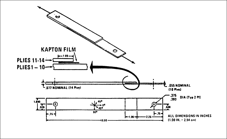
MIL-HDBK-17-1F

Volume 1, Chapter 6 Lamina, Laminate, and Special Form Characterization

6-135

It is a common practice in composites industry to use Mode II value to estimate the criticality of Mode III

fracture.

6.8.6.6 Mixed mode test methods

As discussed in Section 6.8.6.2, in natural delaminations with curved fronts, the energy release rates

not only vary along the front, but mixed mode conditions are also present. Mixed mode effects are also

present in delaminations with straight fronts (edge delaminations and adhesive joints are examples). In

such cases, Mode I and Mode II contributions are dominant, although small Mode III effects may also be

present. For this reason, various attempts have been made to characterize delamination fracture under

combined action of Mode I and Mode II effects and some of them are discussed next.

6.8.6.6.1 Mixed mode specimen or crack lap shear (CLS)

The CLS specimen (Reference 6.8.6.6.1) was patterned after a similar specimen used for bonded

joints. The specimen is a tension coupon, where some of the plies are terminated in the middle of the

coupon (Figure 6.8.6.6.1). This specimen has been used widely in the industry. Mode I and II compo-

nents are computed based on stress analyses (finite element or other methods). Effects of geometric

nonlinearities have also been studied.

FIGURE 6.8.6.6.1 Mixed-mode crack lap shear coupon.

6.8.6.6.2 Mixed mode bending (MMB) test

This test has recently been proposed (References 6.8.6.6.2(a) and (b)) by combining the schemes

used for DCB and ENF tests and the specimen is of the same form as that used in those tests. A special

loading device is utilized, which can produce a wide range of the ratio of Mode I and Mode II components

by changing the lever arm of the device shown in Figure 6.8.6.6.2. Use of the following equations has

been suggested

MIL-HDBK-17-1F

Volume 1, Chapter 6 Lamina, Laminate, and Special Form Characterization

6-136

232

bhLE

6.8.6.6.2(a)

, B

, A

, and B

are expressed by the following equations when a modified linear beam theory is used

for analysis

= (3C-L

)

= (C+L

)

6.8.6.6.2(b)

An ASTM "round robin" test program is planned using the MMB specimen. ASTM subcommittee

D3.06 plans to draft a proposed standard test method based on the results of this test program.

FIGURE 6.8.6.6.2 Mixed-mode-bearing test setup.

6.8.6.6.3 Edge delamination test

This test specimen makes use of a (±

/90

)

tension specimen, in which the free edge effect causes

growth of delamination from the edges (Reference 6.8.6.6.3(a)). However, the delamination growth is

neither uniform nor symmetric, since it does not remain in the midplane, but oscillates vertically between

the 90/-

interfaces. A modified version of the specimen with a starter delamination has been proposed

(Reference 6.8.6.6.3(b)). Data reduction procedures are discussed in References 6.8.6.6.3(a) and (b).

The test has not gained wide acceptance for toughness property determination.

MIL-HDBK-17-1F

Volume 1, Chapter 6 Lamina, Laminate, and Special Form Characterization

6-137

6.8.6.7 Fracture toughness tests for MIL-HDBK-17 data submittal

Data produced by the following test methods (Table 6.8.6.7) are currently being accepted by

MIL-HDBK-17 for consideration for inclusion in Volume 2.

TABLE 6.8.6.7 Fracture toughness test methods for MIL-HDBK-17 data submittal.

Property Symbols Fully Approved, Interim

and Screening Data

Screening

Data Only

Mode I Toughness

ASTM D 5528 --

Mode II Toughness

IIC

ENF --

Mode III Toughness

IIIC

-- --

Mixed Mode I, II Fracture

, G

)

-- MMB

6.9 UNIAXIAL FATIGUE TESTING

Static testing of unidirectional composite specimens is useful for material characterization, compari-

son of materials, and for prediction of application laminate properties through the use of lamination plate

theory. In the area of fatigue, however, no generalized methodology has yet been devised to predict

laminate behavior from unidirectional specimen data. Hence, the development of fatigue design values

becomes a unique problem for each application lay-up. Many studies have been undertaken, and much

has been written concerning life prediction for specific laminates under cyclic loading spectra. Even at

this level, empirical methods have been favored due to the inadequacy of results obtained from cumula-

tive damage models, fracture mechanics analyses, and other theoretical approaches (References 6.9(a)

and (b)).

ASTM Test Method D 3479, "Tension - Tension Fatigue of Oriented Fiber, Resin Matrix Composites",

is a generalized coupon testing method (Reference 6.9(c)). However, because composite fatigue is so

application dependent, it is important that the laminates represent the application and that the laminates

testing account for the service load spectra and environmental conditions. Currently this is accomplished

in composite hardware programs through a "building block" test approach involving coupon, element, and

component specimens, all representative of full-scale structural details.

It is important to note that, for the majority of current aircraft composite structure, fatigue capability

does not become a limiting factor if all static strength concerns have been thoroughly and successfully

addressed. Exceptions to this are high-cycle components such as those found in helicopter dynamic sys-

tems.

6.10 MULTIAXIAL MECHANICAL PROPERTY TESTING

Multiaxial tests, including biaxial and triaxial loadings, can be performed to experimentally evaluate

the effect of combined stress states on composite material response. No standard test methods exist to

MIL-HDBK-17-1F

Volume 1, Chapter 6 Lamina, Laminate, and Special Form Characterization

6-138

guide multiaxial testing, and little data is available. A discussion of multiaxial testing can be found in Vol-

ume 3, Section 10.2.3.2.

6.11 VISCOELASTIC PROPERTIES TESTS

6.11.1 Introduction

The time dependence of the properties of organic matrix composites arises primarily from the visco-

elastic nature of the polymeric matrix resins, which these materials contain. Although these properties are

matrix-dependent, they cannot be simply predicted based upon the viscoelastic properties of the unrein-

forced matrix. Creep compliance, relaxation modulus and even measured glass transition temperature

can vary widely as a function of the content and orientation of reinforcing fibers.

6.11.2 Creep and stress relaxation

Creep is the time-dependent strain exhibited by a material under the action of a constant stress.

Creep is characterized as a function of time by measurement of the creep compliance which is deter-

mined by dividing the time-dependent strain by the level of constant stress. Similarly, stress relaxation is

the time-dependent stress exhibited by a material under the action of a constant strain. The relaxation

modulus is determined by dividing the time-dependent stress by the constant applied strain. Creep and

stress relaxation are different manifestations of the same underlying mechanisms of molecular mobility.

At low levels of applied stress or strain these time-dependent effects may be completely recoverable

when the forcing function is removed, but at higher levels irrecoverable deformations may occur under

load. Irrecoverable strain, sometimes called permanent set, may be accompanied by time-dependent

damage development such as the formation and growth of transverse matrix cracking.

Viscoelastic effects should be considered if the end use involves high stresses in a matrix-dominated

direction, high temperature or exposure to a harsh chemical environment. Composite structural designs

should be evaluated for potential time-dependent effects if the working load involves significant shear

loading. Since high shear loads can be generated near a structural discontinuity, these are areas of po-

tential concern. It should be noted that viscoelastic effects can be beneficial in some of these instances,

since stress relaxation in high stress regions can help prevent catastrophic failure. When a thermoplastic

matrix is employed, time-dependent behavior may be a problem, especially if the service temperature is

at or near

Tg. The extent of creep should be smaller in thermoset composites due to cross-linking.

In fiber-reinforced plastics (composites), one can assume that creep will be more important when the

composite is loaded in a matrix-dominated manner than in a fiber-dominated manner. For instance, the

creep of a unidirectional specimen tensile loaded in the fiber direction is expected to be small and hence

only of secondary importance. However, loading a specimen in a matrix-dominated manner is not as

straight forward as one would expect. Testing a unidirectional specimen in a transverse tensile manner

one would think must essentially load the matrix, and this is not so. There are several explanations. One

of the explanations is that loading a transverse specimen puts the matrix in a bidirectional state of stress

(tensile) because the fibers prevent the matrix from laterally contracting (i.e., Poisson’s effect) and thus

the amount of creep response is restricted. Another argument for low creep response in transverse

specimens is that the specimens are weak and the strains are small, so the change in strain would also

be small. Another way to load the matrix is in shear where the creep response should be large. The most

convenient way to load the matrix in shear is to load a [+

45] specimen in tension. Although there is some

argument that this test does not produce pure intralaminar shear, it at least produces some shearing and

can be thought analogous to loading a unidirectional laminate in shear.

Experience has shown that the resulting creep is significant. Other loadings that would be interesting

to examine with respect to creep response would be compression of unidirectional specimens in the fiber

direction and three-point bend loading of unidirectional specimens (in both of these methods shear plays

a role).

MIL-HDBK-17-1F

Volume 1, Chapter 6 Lamina, Laminate, and Special Form Characterization

6-139

A common experimental procedure is to apply a dead weight tensile load to a [+45] specimen at 5,

10, or 15 ksi (35 MPa, 70 MPa, or 105 MPa) and monitor the strain as a function of time. The strain read-

ing at the first application of the full load is designated as the strain at zero time. Subsequent measure-

ments are timed from that zero time reading. Readings are taken at 1, 2, 3, 10, 20, 30, 60, 100, and 200

minutes, and then as convenience dictates. Strain as a function of time is plotted on semi-log axes and

the test continued for at least 30,000 minutes (or 3 weeks). Testing should be done at controlled (con-

stant) humidity and temperature conditions (References 6.11.2(a) and (b)). Generally, specimens are 1

in. wide, 6 in. long, and ~0.04 – 0.06 in. thick (25 mm wide, 150 mm long and ~1-1.5 mm thick). These

dimensions are open to question; there is some evidence that wider samples will creep less than narrow

samples.

6.12 FORM-SPECIFIC MECHANICAL PROPERTY TESTS

6.12.1 Tests unique to filament winding

6.12.1.1 Overview

The mechanical behavior of filament wound structures is typically different from the behavior of flat

laminated structures. Some noted differences result from the type of cure, resin void content, microcrack-

ing, and free edge construction. However, filament wound structures require the same mechanical prop-

erty data for design and analysis as used for general laminated structures. The majority of filament

wound structures are used in the rocket motorcase community, and consequently, most of the test speci-

mens are in the form of cylinders or bottles that more closely simulate the geometry of the structures to be

designed and analyzed.

6.12.1.2 History

In November 1983, the Joint Army, Navy, NASA, and Air Force (JANNAF) Interagency Propulsion

Committee chartered by the Department of Defense formed the Composite Motorcase Subcommittee

(CMCS) (Reference 6.12.1.2.(a)). The CMCS was concerned with the application of composite materials

in the construction of rocket motorcases for strategic and tactical missiles, space propulsion systems, and

cartridge cases for gun propulsion. The CMCS consisted of four working panels two of which were the

Testing and Inspection (T&I) panel and the Design and Analysis (D&A) panel.

The T&I panel surveyed industry on test methods which resulted in seventeen different tension tests,

seventeen different compression tests and sixteen different shear tests that were being used to obtain

mechanical property data. The T&I and D&A panels joined to evaluate the test methods via a JANNAF

Workshop (Reference 6.12.1.2(b)). A panel of experts in filament wound composites was selected and

tasked to make recommendations for test methods. A joint T&I and D&A Workshop was held in April 1986

to discuss the panel of experts' recommendations and to have an industry selection of JANNAF interim

test standards to be used for the determination of uniaxial material properties.

The CMCS conducted a Design Round Robin (DRR) and a Testing Round Robin (TRR) for three of

the interim tests: 1) Transverse Tension, 2) Transverse Compression and 3) In-plane Shear of ninety de-

gree filament wound cylindrical specimens. The participants in the DRR and the TRR were paid and were

determined through competitive procurement. The manufacturing of the ninety degree filament wound

cylinders and strain gaging were also determined through competitive procurement. Each of the test

specimens were ultrasonically C-scanned for any anomalies. The TRR was conducted in accordance

with ASTM E 691 (Reference 6.12.1.2(c)). The DRR and TRR were successful and resulted in three Mili-

tary Standards in the fall of 1992. The three Military Specifications were put into ASTM format, run

through the balloting phases and approved as ASTM test methods in the fall of 1993. The JANNAF ef-

forts were coordinated with MIL-HDBK-17, ASTM Committee D-30, SACMA, and the DOD Standardiza-

tion Program for Composites Technology.

MIL-HDBK-17-1F

Volume 1, Chapter 6 Lamina, Laminate, and Special Form Characterization

6-140

6.12.1.3 Tension tests for uniaxial material properties

6.12.1.3.1 Zero degree tension

The test method selected for the zero degree tension test is ASTM D 3039 entitled "Standard Test

Method for Tensile Properties of Fiber-Resin Composites" (Reference 6.8.2.2.1(a)). It is recommended

that the test specimens be obtained from a filament wound laminate. The JANNAF CMCS initially voted

on either the pressurized NOL ring or a pressurized ninety degree filament wound tube. There were sev-

eral attempts to obtain valid data from each technique but with little repeatable success.

6.12.1.3.2 Transverse tension

The test method selected to determine the uniaxial material properties for transverse tension is

ASTM D 5450 entitled "Test Method for Transverse Tensile Properties of Hoop Wound Polymer Matrix

Composite Cylinders" (Reference 6.12.1.3.2). This test method was approved as MIL-STD-373 entitled

"Transverse Tensile Properties of Unidirectional Fiber/Resin Composite Cylinders" in the fall of 1992, and

was subsequently approved as an ASTM test method in the fall of 1993.

6.12.1.4 Compression tests for uniaxial material properties

6.12.1.4.1 Zero degree compression

The test method selected to determine zero degree uniaxial material properties is ASTM D 3410 enti-

tled "Test Method for Compressive Properties of Unidirectional or Crossply Fiber-Resin Composites"

(Reference 6.8.3.1(a)). Method B, also known as the IITRI method, is recommended. It is further recom-

mended that the test specimens be obtained from a filament wound laminate.

6.12.1.4.2 Transverse compression

The test method selected to determine the uniaxial material properties for transverse compression is

ASTM D 5449 entitled "Test Method for Transverse Compressive Properties of Hoop Wound Polymer Ma-

trix Composite Cylinders" (Reference 6.12.1.4.2). This test method was approved as MIL-STD-374 enti-

tled "Transverse Compressive Properties of Unidirectional Fiber/Resin Composite Cylinders" in the fall of

1992, and was subsequently approved as an ASTM test method in the fall of 1993.

6.12.1.5 Shear tests for uniaxial material properties

6.12.1.5.1 In-plane shear

The test method selected for the determination of in-plane shear properties is a ninety degree, four

inch diameter filament wound torsion tube described in ASTM D 5448 entitled "Test Method for In-plane

Shear Properties of Hoop Wound Polymer Matrix Composite Cylinders" (Reference 6.12.1.5.1). This test

method was approved as MIL-STD-375 entitled "In-plane Shear Properties of Unidirectional Fiber/Resin

Composite Cylinders" in the fall of 1992, and was subsequently approved as an ASTM test method in the

fall of 1993.

6.12.1.5.2 Transverse shear

The test method selected to determine transverse shear material properties is ASTM D 5379 entitled

"Test Method for Shear Properties of Composite Materials by the V-notched Beam Method" (Reference

6.8.4.2.2(a).

6.12.1.6 Test methods for MIL-HDBK-17 data submittal

Data produced by the following test methods (Table 6.12.1.6) are currently being accepted by MIL-

HDBK-17 for consideration for inclusion in Volume 2 (an element of orientation is shown for clarity).

MIL-HDBK-17-1F

Volume 1, Chapter 6 Lamina, Laminate, and Special Form Characterization

6-141

TABLE 6.12.1.6 Filament wound test methods for MIL-HDBK-17 data submittal.

Property Symbols Fully Approved, Interim,

and Screening Data

Screening

Data Only

0° Tension*

ASTM D 3039 ---

90° Tension*

ASTM D 5450 ---

0° Compression*

ASTM D 3410B ---

90° Compression*

ASTM D 5449 ---

In-Plane Shear**

ASTM D 5448 ---

Transverse Shear***

isu

ASTM D 5379 ---

* Strength, modulus, Poisson's Ratio, and strain

** Strength, modulus, and strain

6.12.2 Tests unique to textiles composites

6.12.2.1 Overview

The physical and mechanical behavior of common textile composites is in many ways similar to that

of the unidirectional materials. Many of the same test methods work in the determination of properties of

the textile composite. This is only applicable to weaves that are homogenous in nature over a small re-

peat length and width. A designer must analyze very large coarse weaves for specific situations that re-

peat over several inches on an individual basis.

In two-dimensional weaves, typical testing concerns are associated with specimen size that defines

the representative structure. In most commercially available fabrics, the repeat is over a small square.

The use of very coarse or odd weave patterns complicates the simplicity of testing allowed by using unidi-

MIL-HDBK-17-1F

Volume 1, Chapter 6 Lamina, Laminate, and Special Form Characterization

6-142

rectional laminate tests. In these large or irregular patterns, it is required to account for repeat sequence

in specimen size selection. Coordinating this within the appropriate test method limitations is sometimes

difficult.

In testing of textile composites, a major factor to consider is z-axis reinforcing. Cross-stitching of two

dimensional textile composites or interconnection of all axes in 3D weaves accomplishes this reinforce-

ment. The cross-stitching and weaving applications introduce reinforcement in the Z-axis to provide bet-

ter properties in the out-of-plane direction. In these textile products, testing must address the

characterization of the third direction. Although a number of programs are investigating the

characterization in the z-direction there is no agreed standard as with the in-plane methods.

For textile processes, the most likely manufacturing defects are associated with porosity and with

“dry” regions from insufficient resin flow. Large planes of weak bonds are unlikely. Conventional ultra-

sonic techniques can detect large areas of porosity. Small areas masked by the inhomogeneous struc-

ture of 3D textiles are possible. The dry regions tend to be on the surface and visually detectable.

There is the possibility of microcracks in the resin rich areas near the tow intersections even in tough-

ened systems. The 3D nature of the materials does not allow for contraction in the Z direction as do 2D

composites so you put a significant 3D stress state on the resin rich areas, hence the potential for cracks

forming.

6.12.2.2 Background

The testing of textile composites is not a new topic. In fact, most of the first composite materials were

reinforced with woven materials. There are numerous reviews of the test methods for unidirectional mate-

rials, but typically the woven materials are as often part of a design as the unidirectional materials. As

discussed previously, test methods for textile composites must account for the pattern associated with

woven textiles to be representative of woven structures.

In typical woven materials, the repeat pattern is less than one tenth of an inch. In these cases testing

per the standard unidirectional methods yields values that are representative of the bulk properties of the

weave. In most instances since the repeating pattern is small, normal testing specimens will accommo-

date the weaving. When using a standard test method developed for a unidirectional laminate, compare

the repeat size to the maximum and typical specimen sizes per the standard test method. If the repeat

pattern is 10X smaller than the specimen test length, no problem should result.

For woven textile fabrics, the pattern is part of the style designation. In glass fabrics, the weavers

number also assigns yarn properties, refer to Reference 6.12.2.2(a) for definition of style numbers of

glass fabric.

In two-dimensional and triaxial braiding this is also true, but the weave comes in the form of a sock.

The reinforcement properties of the sock are created by the tows that are used, the mandrel feed speed

and the diameter and shape of the mandrel. The specimens from a braiding operation require care to

assure the weaving pattern is not changed during the lay-up and impregnation phase of test coupon fabri-

cation.

Tests conducted to evaluate the test specimens used for dry textile preforms and RTM process com-

posites are included in References 6.12.2.2(b) and (c). Section 6.12.2.4 presents discussion of the pecu-

liarities of complex braiding.

6.12.2.3 Fabric and two-dimensional weaves

6.12.2.3.1 Physical property tests

For measuring density and fiber volume fraction of dry composites, the sample should be an order of

magnitude larger than the unit cell size to obtain an average density. For textile composites with average

MIL-HDBK-17-1F

Volume 1, Chapter 6 Lamina, Laminate, and Special Form Characterization

6-143

fiber volume fractions of 0.50 - 0.55, the fiber volume fraction within the yarn can be as large as 0.7.

Thus, use the actual fiber volume fraction in analyses that model the yarns and resin discretely, not aver-

age fiber volume fraction for the textile composite.

Composites made with dry two-dimensional textile preforms used in RTM processes are quasi-

laminar in nature. Thus, a cured ply thickness could be calculated and used for scaling strength with

thickness. For molded parts, the tool volume controls the thickness. The bulk factor (unrestrained thick-

ness/restrained thickness) for a dry preform should be slightly greater than 1:1 to obtain the desired fiber

volume fraction. For bulk factors significantly greater than one, autoclave or press pressures may be re-

quired to close the tool, resulting in unacceptable distortion of the preform. For bulk factors less than one,

the fiber volume fraction will obviously be less than optimum.

6.12.2.3.2 Mechanical testing

The standard test methods found in the static uniaxial mechanical test section (6.8) provide good re-

sults for textile composites made from two-dimensional woven prepreg. However, any testing must take

into account the scale affects associated with the use of textile reinforcements. The repeat size of the

weave dominates this scale affect. If the test specimen size is small enough to be unbalanced, the re-

sults will be unrepresentative of the characterized parts.

As the complexity of the repeat pattern increases, so does the need for larger test specimens. No

specific rule of thumb for this is available and the investigator should evaluate this as part of the program

to establish mechanical values. There are many studies that the reader is encouraged to review as part

of the characterization of the particular weave.

6.12.2.3.3 Impact considerations

The present test methods to measure impact damage tolerance are just as suitable for composite

specimens made from dry textile preforms and a RTM process as composites made from prepreg lami-

nates. One must understand impact response to apply the data. A discussion of impact response is in

Reference 6.12.2.3.3.

6.12.2.4 Complex braiding considerations

The goal of testing braided specimens is to produce mechanical property data that mimics the per-

formance of that section of the braided structure in a representative manner. Often this is difficult to

achieve due to the local contour or details not accurately formed into the test specimens. Therefore, cer-

tain assumptions as to the applicability of the specimens to the final part are necessary before the start of

testing.

Most specimens assume pristine manufacturing in producing the specimen and this is representative

of the final part. This initial coupon may or may not mimic the final product depending upon care and re-

producibility in the design of the part. Test specimens for tension, compression, shear, pin bearing, inter-

laminar shear and interlaminar tension are described in other sections of this handbook. In some cases,

the actual shape of the zone may more accurately represent specimen geometry, i.e., a tapered specimen

(preferably symmetric) that contains the essential geometry of the actual tapered braid.

In general, the specific mechanical properties of interest are torsional stiffness and strength, shear

stiffness and strength, tensile, compressive and flexural moduli and strengths, bearing strength for bolted

assemblies, and adhesive bond strength where required. In the event exposure of the braided parts to

damage or degradation by the environment is possible, a series of tests to provide a measure of the dam-

age tolerance and environmental effects on braided materials must be included. Damage criteria must

include manufacturing defects that are not detectable by non-destructive evaluations.

MIL-HDBK-17-1F

Volume 1, Chapter 6 Lamina, Laminate, and Special Form Characterization

6-144

Several candidate configurations for these types of tests are listed in NASA CR 1092 (Refer-

ence 6.12.2.4) and should be considered as part of a design allowables program based upon intended

use and environment.

Fatigue and creep tests of braided composites are important considerations whenever the part is a

dynamic component. The highly complex courses followed by the braided yarns through the matrix cre-

ate fiber load paths for which stiffnesses and strengths are difficult to predict. The chance that the matrix

is loaded beyond the level predicted by laminated design is high. Therefore, a lower confidence in under-

standing how a braided part behaves will require a rigorous fatigue and creep test plan to characterize the

complex interweave of the braided yarns in the part. Tests designed to determine fatigue or creep effects

are part specific and should be conducted on a braided specimen that is identical to the finished product.

Scaling effects and the use of similitude in test specimen design should be avoided whenever possible.

Otherwise, the results may not mimic a critical defect, which results in a failure of the part before the pre-

dicted value.

In general, it is accurate to state that for both two- and three-dimensional braided composites, defects

are the single most important factor in the design of the part and the corresponding application of the al-

lowables. This is due to the nature of braided preforms as well as physical limitations in the ability of the

yarns to cover an area of rapid change in contour. The good news is that net-shape braided parts do pro-

vide a means to build these parts without intensive hand labor. This makes braiding suitable to produc-

tion environments and fully capable of doing the intended job. This is true when the designer or analyst

has made the correct choices in the type of specimens used for determining braided allowables.

6.12.2.4.1 Three-dimensional weave and braids

Three-dimensional textile composites are typically very complex application driven weavings. The

testing associated with them determines the specific properties addressed by special weavings or cross-

stitching of two-dimensional weaves. Some conventional tests performed on representative sections of

the weave determine and characterize the capabilities of these processes. Currently there are many in-

vestigations under way to standardize tests in the z-axis but no industry standard has yet been set.

6.12.2.4.2 Through the thickness test methods

Many methods have been developed to characterize the through the thickness properties. Interlami-

nar test methods are desirable for optimizing the type and amount of through the thickness reinforcement

in textile composites; Table 6.12.2.4.2 shows commonly used methods. These test methods must have

additional work before recommending them for standardization. None of the in-plane shear test methods

was totally acceptable. A review of those investigations is in Reference 6.12.2.3.3.

6.12.2.5 Test methods for submission to MIL-HDBK-17

In general, the methods described in the preceding sections on unidirectional materials should be

used to characterize textile composites. These are only applicable to weaves that are homogenous in

nature over a small repeat length and width. Very large coarse weave repeats developed for specific

situations are beyond the scope of this section and the handbook. Analyze these weaves for testing on

an individual basis.

For appropriate test methods for individual test conditions see the following sections:

Tension test methods 6.8.2.4

Compression test methods 6.8.3.4

Shear test methods 6.8.4.4

Fracture toughness tests 6.8.6.7

MIL-HDBK-17-1F

Volume 1, Chapter 6 Lamina, Laminate, and Special Form Characterization

6-145

6.12.3 Tests unique to thick-section composites

No standard test methods exist to guide thick-section testing, and little data is available. Mechanical

tests, including uniaxial, biaxial, and triaxial loadings, can be performed to experimentally evaluate the

effect of combined stress states on composite material response. A discussion of thick-section testing

can be found in Volume 3, Section 7.2.3.

TABLE 6.12.2.4.2 Proposed in-plane shear tests methods for 3D reinforced composites.

Test method type Test Method

Specification

Test Method Title Comments

Shear ASTM E 143 Standard Test Method for Shear

Modulus at Room Temperature

Reference 6.12.2.4.2

ASTM D 4255 Standard Guide for Testing In-

plane Shear Properties of

Composite Laminates

None Compact Shear

Interlaminar tension ASTM D 6415 Standard Test Method for

Measuring the Curved Beam

Strength of a Fiber-Reinforced

Polymer-Matrix Composite

Interlaminar fracture

toughness

ASTM D 5528 Standard Test Method for Mode

I Interlaminar Fracture

Toughness of Unidirectional

Fiber-Reinforced Polymer

Matrix Composites

Reasonable for 2-D

braids and stitched

uniweaves

Interlaminar fracture

toughness

See 6.8.6.4.1 End Notched Flexure (Mode II) Reasonable for 2-D

braids

Interlaminar tension ASTM C 297 Standard Test Method for

Flatwise Tensile Strength of

Sandwich Constructions

Reasonable for elastic

constants

Interlaminar

compression

ASTM D 3410,

Procedure B

Standard Test Method for

Compressive Properties of

Polymer Matrix Composite

Materials with Unsupported

Gage Section by Shear Loading

Reasonable for elastic

constants and strength

Interlaminar shear None Compact Reference 6.12.2.4.2,

Thick composites

ASTM D 3846 Standard Test Method for In-

Plane Shear Strength of

Reinforced Plastics

Thin composites

Interlaminar shear -

transverse

ASTM D 2344 Standard Test Method for Short-

Beam Strength of Polymer

Matrix Composite Materials and

Their Laminates

Reasonable for 2-D

braids and 3-D weaves

MIL-HDBK-17-1F

Volume 1, Chapter 6 Lamina, Laminate, and Special Form Characterization

6-146

6.13 SPACE ENVIRONMENTAL EFFECTS ON MATERIAL PROPERTIES

This section is reserved for future use.

6.13.1 Introduction

This section is reserved for future use.

6.13.2 Atomic oxygen

This section is reserved for future use.

6.13.3 Micrometeoroid Debris

This section is reserved for future use.

6.13.4 Ultraviolet radiation

This section is reserved for future use.

6.13.5 Charged particles

This section is reserved for future use.

MIL-HDBK-17-1F

Volume 1, Chapter 6 Lamina, Laminate, and Special Form Characterization

6-147

REFERENCES

6.3.1 ASTM Test Method D 5229/D 5229M, “Moisture Absorption Properties and Equilibrium

Conditioning of Polymer Matrix Composite Materials,” Annual Book of ASTM Standards,

Vol 15.03, American Society for Testing and Materials, West Conshohocken, PA.

6.3.2(a) ASTM Practice D 618, “Conditioning of Plastics and Electrical Insulating Materials for Test-

ing,” Annual Book of ASTM Standards, Vol 8.01, American Society for Testing and Materi-

als, West Conshohocken, PA.

6.3.2(b) ASTM Test Method D 570, “Water Absorption of Plastics,” Annual Book of ASTM Stan-

dards, Vol 8.01, American Society for Testing and Materials, West Conshohocken, PA.

6.3.2(c) SACMA Recommended Method (SRM) 11-88, “Recommended Procedure for Conditioning

of Composite Test Laminates,” Suppliers of Advanced Composite Materials Association, Ar-

lington, VA.

6.3.3(a) Ryder, J. T., “Effect of Load History on Fatigue Life,” AFWAL-TR-80-4044, July, 1980.

6.3.3(b) SACMA Recommended Method (SRM) 11R-94, “Recommended Method for Environmental

Conditioning of Composite Test Laminates,” Suppliers of Advanced Composite Materials

Association, Arlington, VA.

6.3.3.2 Weisman, S., “Relative Humidity Measurement Errors in Environmental Test Chambers,”

Test Engineering & Management, October/November 1990, pg. 16-17.

6.4.1 ASTM Practice E 83-94, "Practice for Verification and Classification of Extensometers,"

Annual Book of ASTM Standards, Volume 3.01, American Society for Testing and Materi-

als, West Conshohocken, PA .

6.4.2.8 ISO 10012-1:1992 "Quality Assurance Requirements for Measuring Equipment -- Part 1:

Metrological Confirmation System for Measuring Equipment."

6.4.3.1(a) ASTM E-4, “Standard Practices for Force Verification of Testing Machines,” Annual Book of

ASTM Standards, Vol 3.01, American Society for Testing and Materials, West Consho-

hocken, PA, ISBN 0-8031-1915-1.

6.4.3.1(b) ASTM E-74, “Standard Practice of Calibration of Force-Measuring Instruments for Verifying

the Force Indication of Testing Machines,” Annual Book of ASTM Standards, Vol 3.01,

American Society for Testing and Materials, West Conshohocken, PA, ISBN 0-8031-1915-

6.4.3.1(c) ASTM E-467, “Standard Practice for Verification of Constant Amplitude Dynamic Loads on

Displacements in an Axial Load Fatigue Testing System,” Annual Book of ASTM Standards,

Vol 3.01, American Society for Testing and Materials, West Conshohocken, PA, ISBN 0-

8031-1915-1.

6.4.3.1(d) ISO 5893, “Rubber and Plastics Test Equipment – Tensile, Flexural and Compressive

Types (Constant Rate of Traverse) – Description,” International Organization for Standardi-

zation, Geneva, Switzerland.

6.4.3.3 Window and Hollister, “Strain Gage Technology,” Applied Science Publishers, Essex, Eng-

land, ISBN 0-85334-118-4, p. 267.

6.4.4.4 G. Sines, Elasticity and Strength, Allyn & Bacon Inc. 470 Atlantic Ave, Boston MA LCCN:

69-14637.

MIL-HDBK-17-1F

Volume 1, Chapter 6 Lamina, Laminate, and Special Form Characterization

6-148

6.4.4.4.1(a) “Temperature Induced Apparent Strain and Gage Factor Variation in Strain Gages,” Tech

Note TN-504-1. Available free of charge from: Measurements Group Inc. P.O. Box 27777

Raleigh, NC 27611. Measurements Group makes available an extensive collection of tech

notes and tips relating to strain measurement, all are available at no charge.

6.4.4.4.1(b) “Strain Gage Selection Criteria, Procedures, Recommendations,” Tech Note TN-505-2.

Available free of charge from: Measurements Group Inc. P.O. Box 27777 Raleigh, NC

27611

6.4.4.4.2 "Surface Preparation for Strain Gage Bonding," M-LINE ACCESSORIES Instruction Bulle-

tin B-129-6, Micro-Measurements Division, Measurements Group Inc. P.O. Box 27777, Ra-

leigh, NC 27611, USA

6.4.4.4.4 "Optimizing Strain Gage Excitation Levels," Tech Note TN-502. Available free of charge

from: Measurements Group Inc. P.O. Box 27777 Raleigh, NC 27611.

6.4.4.4.5.1 "Shunt Calibration of Strain Gage Instrumentation," Tech Note TN-514. Available free of

charge from: Measurements Group Inc. P.O. Box 27777 Raleigh, NC 27611.

6.4.4.6(a) Mechanics of Textile Composites Conference. NASA CP 3311, Parts 1 & 2, Oct. 1995.

6.4.4.6(b) Masters, John E., and Portanova, Marc A., “Standard Test Methods for Textile Composites,”

NASA CR-4751, Sept. 1996 (URL http://techreports.larc.nasa.gov/ltrs).

6.4.5.9(a) “The Temperature Handbook”, Volume 29, Omega Engineering, Inc. 1995.

6.4.5.9(b) “Guidelines for Realizing the International Temperature Scale of 1990 (ITS-90), B.W. Mag-

num and G.T. Furukawa, National Institute of Standards and Technology.

6.4.5.9(c) ASTM E220-86 (reapproved 1996) Calibration of Thermocouples by Comparison Tech-

niques.

6.4.5.9(d) ASTM E77-92 Standard Test Method for Inspection and Verification of Thermometers.

6.4.5.9(e) ASTM E1502- ASTM E1502 Use of Freezing Point Cells for Reference Temperatures.

6.6.3.1 Young, R.J., Introduction to Polymers, Section 4.4.2, Chapman and Hall, 1981, pp. 199-

202.

6.6.3.2.1 ASTM Test Method E 1356-91, "Glass Transition Temperatures by Differential Scanning

Calorimetry or Differential Thermal Analysis," Annual Book of ASTM Standards, Vol 14.02,

American Society for Testing and Materials, West Conshohocken, PA.

6.6.3.2.3(a) ASTM Practice D 4065-85, "Standard Practice for Determining and Reporting Dynamic

Mechanical Properties of Plastics," Annual Book of ASTM Standards, Vol 8.02, American

Society for Testing and Materials, West Conshohocken, PA.

6.6.3.2.3(b) SACMA Recommended Method (SRM) 18R-94, "Recommended Method for Glass Transi-

tion Temperature (T

) Determination by DMA of Oriented Fiber-Resin Composites," Suppli-

ers of Advanced Composite Materials Association, Arlington, VA.

6.6.4.1(a) ASTM D 792, “Standard Test Method for Density and Specific Gravity (Relative Density) of

Plastics by Displacement,” Annual Book of ASTM Standards, ASTM, West Conshohocken,

PA.

MIL-HDBK-17-1F

Volume 1, Chapter 6 Lamina, Laminate, and Special Form Characterization

6-149

6.6.4.1(b) ASTM D 1505, “Standard Test Method for Density of Plastics by the Density-Gradient Tech-

nique,” Annual Book of ASTM Standards, ASTM, West Conshohocken, PA.

6.6.4.1(c) ASTM D 4892, "Standard Test Method for Density of Solid Pitch (Helium Pycnometer

Method), Annual Book of ASTM Standards, ASTM, West Conshohocken, PA.

6.6.4.1(d) ASTM D2734, “Standard Test Method for Void Content of Reinforced Plastics,” Annual

Book of ASTM Standards, ASTM, West Conshohocken, PA.

6.6.4.1(e) Ghiorse, S.R., data presented to MIL-HDBK-17 PMC Testing Working Group, Santa Fe,

NM, March 1996.

6.6.4.1(f) Ghiorse, S.R. and Tiffany, J, “Evaluation of Gas Pycnometry as a Density Measurement

Method,” Proceedings of the 34th MIL-HDBK-17 PMC Coordination Group, Schaumberg,

IL, September 1996.

6.6.4.2(a) In-progress revision of ASTM D 3171, currently titled, "Standard Test Method for Fiber Con-

tent of Resin-Matrix Composites by Matrix Digestion," D-30 Committee, Spring 1997

D30.03 subcommittee ballot.

6.6.4.2(b) ASTM D 5229/D 5229M, "Standard Test Method for Moisture Absorption Properties and

Equilibrium Conditioning of Polymer Matrix Composites," Annual Book of ASTM Standards,

ASTM, West Conshohocken, PA.

6.6.4.3 Ghiorse, S.R., “A Comparison of Void Measurement Methods for Carbon/Epoxy Compos-

ites,” U.S. Army Materials Technology Laboratory, TR 91-13, April 1991.

6.6.4.4 ASTM D 4892, "Standard Test Method for Density of Solid Pitch (Helium Pycnometer

Method), Annual Book of ASTM Standards, ASTM, West Conshohocken, PA.

6.6.4.4.1(a) ASTM D 618, "Standard Practice for Conditioning Plastics and Electrical Insulating Materi-

als for Testing," Annual Book of ASTM Standards, ASTM, West Conshohocken, PA.

6.6.4.4.1(b) Standard Reference Materials Program, National Institute of Standards and Technology,

Gaithersburg, MD 20899-0001.

6.6.5.3(a) ASTM E 797-90 "Standard Practice for Measuring Thickness by Manual Ultrasonic Pulse-

Echo Contact Method," 1993 Annual Book of ASTM Standards, Vol 3.03, Philadelphia, PA,

1993.

6.6.5.3(b) SACMA Recommended Method (SRM) 24R-94, "Recommended Method for Determination

of Resin Content, Fiber Areal Weight and Flow of Thermoset Prepreg by Combined Me-

chanical and Ultrasonic Methods," Suppliers of Advanced Composite Materials Associa-

tion, Arlington, VA.

6.6.5.4 SACMA Recommended Method (SRM) 10R-94, "Recommended Method for Fiber Volume,

Percent Resin Volume and Calculated Average Cured Ply Thickness of Plied Laminates,"

Suppliers of Advanced Composite Materials Association, Arlington, VA.

6.6.6.2(a) ASTM Test Method D 3171-76, "Fiber Content of Resin-Matrix Composites by Matrix Di-

gestion," Annual Book of ASTM Standards, Vol 15.03, American Society for Testing and

Materials, West Conshohocken, PA.

MIL-HDBK-17-1F

Volume 1, Chapter 6 Lamina, Laminate, and Special Form Characterization

6-150

6.6.6.4(a) SACMA Recommended Method (SRM) 10R-94, “Recommended Method for Fiber Volume,

Percent Resin Volume and Calculated Average Cured Ply Thickness of Plied Laminates,”

Suppliers of Advanced Composite Materials Association, Arlington, VA.

6.6.6.4(b) Kelly, K.M. and Ciriscioli, P.R., “A Non-Destructive Test Method for the Determination of

Percent Resin Content, Fiber Areal Weight and Percent Fiber Volume of Composite Mate-

rials,” Proceedings of the 43

SAMPE Symposium and Exhibition, Anaheim, CA, June,

1998.

6.6.7.2 ASTM Test Method D 2734-70 "Void Content of Reinforced Plastics," Annual Book of

ASTM Standards, Vol 8.02, American Society for Testing and Materials, West Consho-

hocken, PA.

6.6.8.1(a) ASTM D 5229/D 5229M-92, Test Method for Moisture Absorption Properties and Equilib-

rium Conditioning of Polymer Matrix Composite Materials.

6.6.8.1(b) SACMA SRM 11R-94, Environmental Conditioning of Composite Test Laminates.

6.6.8.1(c) Environmental Effects on Composite Materials, George S. Springer, Ed., Technomic Pub-

lishing Co., 1981.

6.6.9.1.2(a) ASTM Test Method D 696-98, “Test Method for Coefficient of Linear Thermal Expansion of

Plastics Between –300C and 30C,” Annual Book of ASTM Standards, Vol. 8.01, American

Society for Testing and Materials, West Conshohocken, PA.

6.6.9.1.2(b) ASTM Test Method E 228-95, “Test Method for Linear Thermal Expansion of Solid Materi-

als With a Vitreous Silica Dilatometer,” Annual Book of ASTM Standards, Vol. 14.02,

American Society for Testing and Materials, West Conshohocken, PA.

6.6.9.1.2(c) ASTM Test Method E 831-93, “Test Method for Linear Thermal Expansion of Solid Materi-

als by Thermomechanical Analysis,” Annual Book of ASTM Standards, Vol. 4.11, American

Society for Testing and Materials, West Conshohocken, PA.

6.6.9.1.2(d)) ASTM Test Method E 289-99, “Test Method for Linear Thermal Expansion of Rigid Solids

with Interferometry,” Annual Book of ASTM Standards, Vol. 14.02, American Society for

Testing and Materials, West Conshohocken, PA.

6.6.9.1.2(e) Yaniv, G., Peimanidis, G., and Daniel, I.M., “Method for Hygromechanical Characterization

of Graphite/Epoxy Composite,” Journal of Composites Technology & Research, Vol. 9,

1987, pp. 21-25.

6.6.9.2.1(a) Fukuda, M., Ochi, M., Miyagawa, M., and Kawai, H., “Moisture Sorption Mechanism of

Aromatic Polyamide Fibers: Stoichiometry of the Water Sorbed in Poly(para-phenylene Ter-

ephthalamide) Fibers,”, Textile Research Journal, Vol. 61, No. 11, 1991, pp. 668-680.

6.6.9.2.1(b) Piggott, M.R., “Water Absorption in Carbon and Glass Fibre Composites,” Paper No. 4.180,

Proceedings of ICCM/VI and ECCM/II, Elsevier Applied Science, Publishers, London,

1987.

6.6.9.2.1(c) Tsai, C-L, and Chiang, C-H., “Characterization of the Hygric Behavior of Single Fibers,”

Composites Science and Technology, Vol. 60, 2000, pp. 2725-2729.

6.6.9.2.1(d) Cairns, D.S., and Adams, D.F., “Moisture and Thermal Expansion of Composite Materials,”

Report UWME-DR-101-104-1, Department of Mechanical Engineering, University of Wyo-

ming, Laramie, WY, November 1981.

MIL-HDBK-17-1F

Volume 1, Chapter 6 Lamina, Laminate, and Special Form Characterization

6-151

6.6.9.2.1(e) Cairns, D.S., and Adams, D.F., “Moisture and Thermal Expansion Properties of Unidirec-

tional Composite Materials and the Epoxy Matrix,” Journal of Reinforced Plastics and Com-

posites, Vol. 2, No. 4, October 1983, pp. 239-255.

6.6.9.2.1(f) Norris, M.A., and Wolff, E.G., “Moisture Expansion Measurement and Data Analysis Tech-

niques for Composite Structures,” Materials Challenge, Diversification and the Future, D.

Hamston, R. Carson, G.D. Bailey, and F.J. Riel, Editors, 40

International SAMPE Sympo-

sium, Anaheim, CA, May 8-11, 1995, pp. 1867-1878.

6.6.9.2.1(g) Wolff, E.G., Chen, H., and Oakes, D.W., “Hygrothermal Deformation of Composite Sand-

wich Panels,” Advanced Composite Letters, Vol. 9, No. 1, 2000, pp. 35-43.

6.6.9.2.1(h) Wolff, E.G., Chen, H., and Oakes, D.W., “Hygrothermal Deformation of Composite Sand-

wich Panels,” Proceedings of the 12

International Conference on Composite Materials

(ICCM/XII), 1999; also, Society of Manufacturing Engineers Technical Paper No. EM00-

246, Dearborn, MI, 2000.

6.6.9.2.1(i) ASTM Test Method 481-99, “Test Method for Laboratory Aging of Sandwich Constructions,”

Annual Book of ASTM Standards, Vol. 15.03, American Society for Testing and Materials,

West Conshohocken, PA.

6.6.9.2.1(j) ASTM D 5229/D 5229M-92 (1998), “Test Method for Moisture Absorption Properties and

Equilibrium Conditioning of Polymer Matrix Composite Materials,“ Annual Book of ASTM

Standards, Vol. 15.03, American Society for Testing and Materials, West Conshohocken,

PA.

6.6.9.2.1(k) ASTM E 104-85 (1996), “Practice for Maintaining Constant Relative Humidity by Means of

Aqueous Solutions,” Annual Book of ASTM Standards, Vol. 11.03, American Society for

Testing and Materials, West Conshohocken, PA.

6.6.9.2.1(l) Wolff, E.G., “Prediction of Non-Mechanical Transient Strains in Polymer Matrix Compos-

ites,” Paper No. 32-S, Composites, Design, Manufacture and Applications, Proceedings of

the 8

International Conference on Composite Materials (ICCM/VIII), S.W. Tsai and G.S.

Springer, Editiors, 1991.

6.6.10.2.1(a) ASTM C177-97 “Steady-State Heat Flux Measurements and Thermal Transmission Proper-

ties by Means of the Guarded-Hot-Plate Apparatus,” 1997 Annual Book of ASTM Stan-

dards, Vol 04.06, ASTM, Philadelphia, PA.

6.6.10.2.1(b) ASTM C1044-97, “Practice for Using the Guarded-Hot-Plate Apparatus in the One-Sided

Mode to Measure Steady-State Heat Flux and Thermal Transmission Properties,” Annual

Book of ASTM Standards, Vol 04.06, ASTM, Philadelphia, PA.

6.6.10.2.2 ASTM E1225-99 “Thermal Conductivity of Solids by Means of the Guarded-Comparative-

Longitudinal Heat Flow Technique,” Annual Book of ASTM Standards, Vol 14.02, ASTM,

Philadelphia, PA.

6.6.10.2.3(a) ASTM C518-98 “Steady-State Thermal Transmission Properties by Means of the Heat Flow

Meter Apparatus,” Annual Book of ASTM Standards, Vol 04.06, ASTM, Philadelphia, PA.

6.6.10.2.3(b) ASTM C1046-98 “Practice for In-Situ Measurement of Heat Flux and Temperature of

Building Envelope Components,” Annual Book of ASTM Standards, Vol 04.06, ASTM,

Philadelphia, PA.

MIL-HDBK-17-1F

Volume 1, Chapter 6 Lamina, Laminate, and Special Form Characterization

6-152

6.6.10.2.3(c) ASTM E1530-93 “Standard Test Method for Evaluating the Resistance to Thermal Trans-

mission of Thin Specimens of Materials by the Guarded Heat Flow Meter Technique,” An-

nual Book of ASTM Standards, Vol 04.06, ASTM, Philadelphia, PA.

6.6.11.2 ASTM E1269-95, “Determining Specific Heat Capacity by Differential Scanning Calo-

rimetry,” 1995 Annual Book of ASTM Standards, 14.02, ASTM, Philadelphia, PA.

6.6.11.2.1 Differential Scanning Calorimetry, J. L. McNaughton and C. T. Mortimer, Perkin Elmer Or-

der Number L-604, reprinted from “IRS; Physical Chemistry Series 2, 1975, Volume 10,”

which was taken with permission of the publisher Butterworths, London, p. 12.

6.6.12.2(a) ASTM E1461-92 “Thermal Diffusivity of Solids by the Flash Method,” Annual Book of

ASTM Standards, Vol 14.02, ASTM, Philadelphia, PA.

6.6.12.2(b) ASTM C714-85 “Thermal Diffusivity of Carbon and Graphite By a Thermal Pulse Method,”

Annual Book of ASTM Standards, 15.01 ASTM, Philadelphia, PA.

6.6.13(a) NASA CR-4740, “Contamination Control Engineering Design Guidelines for the Aerospace

Community”, AC Tribble et al, eds., NASA CASI, Linthicum Heights, MD, 1996

6.6.13(b) NASA RP-1124, Revision 3, “Outgassing Data for Selecting Spacecraft Materials”, WA

Campbell, JJ Scialdone, eds., NASA CASI, Linthicum Heights, MD, 1993, maintained on-

line by the Goddard Space Flight Center at http://epims.gsfc.nasa.gov/og/

6.6.13(c) MAPTIS, online database maintained by the Marshall Space Flight Center at

http://map1.msfc.nasa.gov

6.7.1(a) ASTM Test Method D 149-93a, “Dielectric Breakdown Voltage and Dielectric Strength of

Solid Electrical Insulating Materials,” Annual Book of ASTM Standards, Vol 10.01, Ameri-

can Society for Testing and Materials, West Conshohocken, PA.

6.7.1(b) ASTM Test Method D 150-93, “A-C Loss Characteristics and Permittivity (Dielectric Con-

stant) of Solid Electrical Insulating Materials,” Annual Book of ASTM Standards, Vol 10.01,

American Society for Testing and Materials, West Conshohocken, PA.

6.7.1(c) ASTM Test Method D 495-89, “High-Voltage, Low-Current, Dry Arc Resistance of Solid

Electrical Insulation,” Annual Book of ASTM Standards, Vol 10.01, American Society for

Testing and Materials, West Conshohocken, PA.

6.7.1(d) ASTM Test Method D 2303-90, “Liquid Contaminant, Inclined-Plane Tracking, and Erosion

of Insulating Materials,” Annual Book of ASTM Standards, Vol 10.01, American Society for

Testing and Materials, West Conshohocken, PA.

6.6.18.1(a) Sorathia, U., Lyon, Richard, Ohlemiller, Thomas, and Grenier, Lt. Andrew, “ A Review of

Fire Test Methods and Criteria for Composites”, SAMPE Journal, Vol 33, No.4, July/August

1997.

6.6.18.1(b) Ohlemiller T., and Cleary, T., "Upward Flame Spread on Composite Materials”, Chapter 28

in Fire and Polymers II- Materials And Tests for Hazard Prevention, (G. L. Nelson, ed.)

American Chemical Society, Washington, DC, 1995, pp. 422-434.

6.6.18.1(c) Ohlemiller, T., Cleary, T. and Shields, J., “Effect of Ignition Conditions on Upward Flame

Spread on a Composite Material in a Corner Configuration”, Proceedings of the 41st Inter-

national SAMPE Symposium, Society for the Advancement of Material and Process Engi-

neering, Covina, CA, 1996, p. 734.

MIL-HDBK-17-1F

Volume 1, Chapter 6 Lamina, Laminate, and Special Form Characterization

6-153

6.6.18.2(a) Grand, A, "Fire Evaluation of Coatings for Glass-Reinforced Polymeric Composites", Pro-

ceedings of Fire and Materials, 2nd International Conference, Interscience Communica-

tions Ltd., London, 1993, p. 144.

6.6.18.2(b) Sorathia U., and Beck, C., “Fire Protection of Glass/vinyl Ester Composites for Structural

Applications”, Proceedings of the 41st International SAMPE Symposium, Society for the

Advancement of Material and Process Engineering, Covina, CA, 1996.

6.6.18.2(c) Ohlemiller, T and Shields, J., “The Effect of Surface Coatings on Fire Growth over Com-

posite material”, National Institute of Standards and Technology NISTIR 5940, December

1996.

6.6.18.2(d) DOT/FAA/AR-00/12, Aircraft Material Fire Test Handbook, U.S. Department of Transporta-

tion, Federal Aviation Administration Technical Center, Atlantic City, NJ 08405.

6.6.18.2.1 ASTM E 84-00a, “Standard Test Method for Surface Burning Characteristics of Building

Materials,” Annual Book of ASTM Standards, Vol 4.07, American Society for Testing and

Materials, West Conshohocken, PA.

6.6.18.2.2 ASTM E 162-98, “Standard Test Method for Surface Flammability of Materials Using a Ra-

diant Heat Energy Source,” Annual Book of ASTM Standards, Vol 4.07, American Society

for Testing and Materials, West Conshohocken, PA.

6.6.18.2.3 ISO 9705, Fire tests-Full-scale room test for surface products, International Organization

for Standardization, Geneva, Switzerland.

6.6.18.2.4 ASTM E 1321-97a, “Standard Test Method for Determining Material Ignition and Flame

Spread Properties,” Annual Book of ASTM Standards, Vol 4.07, American Society for Test-

ing and Materials, West Conshohocken, PA.

6.6.18.3(a) Babrauskas, V., Levin, B., Gann, R., Paabo, M., Harris, R., Peacock, R., and Yusa, S.,

“Toxic Potency Measurement for Fire Hazard Analysis”, National Institute of Standards and

Technology Special Publication 827, December 1991.

6.6.18.3(b) Sorathia, U., Lyon, R., Gann, R.G., Gritzo, L., “ Materials and Fire Threat”, Fire Technology,

Vol 33, Number 3, Sept/Oct 1997.

6.6.18.3.1 ASTM E 662-97, “Standard Test Method for Specific Optical Density of Smoke Generated

by Solid Materials,” Annual Book of ASTM Standards, Vol 4.07, American Society for Test-

ing and Materials, West Conshohocken, PA.

6.6.18.3.2 NFPA 269, Standard Test Method for Developing Toxic Potency Data for Use in Fire Haz-

ard Modeling, National Fire Protection Association, 1 Batterymarch Park, Quincy, MA

02269-9101.

6.6.18.4(a) IMO Resolution MSC.40(64), "Standard for Qualifying Marine Materials for High Speed

Craft as Fire-Restricting Materials", International Maritime Organization, London, Decem-

ber, 1994.

6.6.18.4(b) MIL-STD-2031(SH), "Fire and Toxicity Test Methods And Qualification Procedure For Com-

posite Material Systems Used in Hull, Machinery, and Structural Applications Inside Naval

Submarines", February 1991.

6.6.18.4.1 ASTM E 1354-99, “Standard Test Method for Heat and Visible Smoke Release Rates for

Materials and Products Using an Oxygen Consumption Calorimeter,” ,” Annual Book of

MIL-HDBK-17-1F

Volume 1, Chapter 6 Lamina, Laminate, and Special Form Characterization

6-154

ASTM Standards, Vol 4.07, American Society for Testing and Materials, West Consho-

hocken, PA.

6.6.18.4.2 ASTM E 906-99, “Standard Test Method for Heat and Visible Smoke Release Rates for

Materials and Products,” Annual Book of ASTM Standards, Vol 4.07, American Society for

Testing and Materials, West Conshohocken, PA.

6.6.18.5(a) Sarkos, C.P., and Hill, R.G., “Heat Exposure and Burning Behavior of Cabin Materials Dur-

ing an Aircraft Post-Crash Fuel Fire”, National Materials Advisory Board, National Research

Council, NMAB Report 477-2, National Academy Press, 25, 1995.

6.6.18.5(b) Petrie, George L., Sorathia, Usman, Warren, L. Will, “Testing and Analysis of Marine Com-

posite Structures in Elevated Temperature Conditions”, Proceedings of the 44th Interna-

tional SAMPE Symposium, Vol 44, May 23-27, 1999.

6.6.18.5.1 ASTM E-119-00a, “Standard Test Method for Fire Tests of Building Construction and Mate-

rials,” ,” Annual Book of ASTM Standards, Vol 4.07, American Society for Testing and Mate-

rials, West Conshohocken, PA.

6.6.18.5.2(a) ASTM E-1529-00, “Standard Test Method for Determining Effects of Large Hydrocarbon

Pool Fires on Structural Members and Assemblies,” ,” Annual Book of ASTM Standards,

Vol 4.07, American Society for Testing and Materials, West Conshohocken, PA.

6.6.18.5.2(b) UL 1709, Rapid Rise Fire Tests of Protection Materials for Structural Steel, Underwriters

Laboratories Inc., 333 Pfingsten Road, Northbrook, IL 60062-2096.

6.8.2.2.1(a) ASTM Test Method D 3039/D 3039M, "Tensile Properties of Polymer Matrix Composites,"

Annual Book of ASTM Standards, Vol 15.03, American Society for Testing and Materials,

West Conshohocken, PA.

6.8.2.2.1(b) ISO 527, “Plastics --- Determination of Tensile Properties,” American National Standards

Institute, available from ANSI, 11 W. 42nd Street, New York, NY, 10036.

6.8.2.2.1(c) SACMA Recommended Method (SRM) 4, "Tensile Properties of Oriented Resin-Matrix

Composites," Suppliers of Advanced Composites Materials Association, Arlington, VA.

6.8.2.2.1(d) SACMA Recommended Method (SRM) 9, "Tensile Properties of Oriented Resin-Matrix

Crossply Laminates," Suppliers of Advanced Composite Materials Association, Arlington,

VA.

6.8.2.2.1(e) ASTM Test Method D 5083, "Tensile Properties of Reinforced Thermosetting Plastics Using

Straight-Sided Specimens," Annual Book of ASTM Standards, Vol 8.03, American Society

for Testing and Materials, West Conshohocken, PA.

6.8.2.2.3(a) ASTM Test Method D 638, "Tensile Properties of Plastics," Annual Book of ASTM Stan-

dards, Vol 8.01, American Society for Testing and Materials, West Conshohocken, PA.

6.8.2.2.3(b) SAE AMS 3844A, "Cloth, Type 'E' Glass, Style 7781 Fabric, Hot-Melt, Addition-Type, Poly-

imide Resin Impregnated," Society of Automotive Engineers, Warrendale, PA.

6.8.2.2.4 ASTM Test Method D 2290, "Apparent Tensile Strength of Ring or Tubular Plastics and Re-

inforced Plastics by Split Disk Method," Annual Book of ASTM Standards, Vol 8.04, 15.03,

American Society for Testing and Materials, West Conshohocken, PA.

MIL-HDBK-17-1F

Volume 1, Chapter 6 Lamina, Laminate, and Special Form Characterization

6-155

6.8.2.2.5 ASTM Test Method C 393, "Flexural Properties of Flat Sandwich Constructions," Annual

Book of ASTM Standards, Vol 15.03, American Society for Testing and Materials, West

Conshohocken, PA.

6.8.2.3.2(a) ASTM Test Method C 297, "Tensile Strength of Flat Sandwich Constructions in the Flatwise

Plane," Annual Book of ASTM Standards, Vol 15.03, American Society for Testing and Ma-

terials, West Conshohocken, PA.

6.8.2.3.2(b) ASTM Test Method C 633, "Adhesive or Cohesive Strength of Flame Sprayed Coatings,"

Annual Book of ASTM Standards, Vol 15.03, American Society for Testing and Materials,

West Conshohocken, PA.

6.8.2.3.2(c) ASTM Test Method D 2095, "Tensile Strength of Adhesives by Means of Bar and Rod

Specimens," Annual Book of ASTM Standards, Vol 15.06, American Society for Testing and

Materials, West Conshohocken, PA.

6.8.2.3.3 Jackson, W. C. and Martin, R. H, “An Interlaminar Tensile Strength Specimen,” ASTM STP

1206, American Society for Testing and Materials, 1993.

6.8.3.1(a) ASTM Test Method D 3410-95, “Compressive Properties of Polymer Matrix Composite Ma-

terials with Unsupported Gage Section by Shear Loading,” Annual Book of ASTM Stan-

dards, Vol 15.03, American Society for Testing and Materials, West Conshohocken, PA.

6.8.3.1(b) ASTM Test Method D 5467-97, “Compressive Properties of Unidirectional Polymer Matrix

Composites Using a Sandwich Beam,” Annual Book of ASTM Standards, Vol 15.03, Ameri-

can Society for Testing and Materials, West Conshohocken, PA.

6.8.3.1(c) ASTM Test Method D 695-96, “Compressive Properties of Rigid Plastics,” Annual Book of

ASTM Standards, Vol 8.01, American Society for Testing and Materials, West Consho-

hocken, PA.

6.8.3.1(d) SACMA Recommended Method (SRM) 1R-94, “Compressive Properties of Oriented Fiber-

Resin Composites, “ Suppliers of Advanced Composite Materials Association, Arlington,

VA.

6.8.3.1(e) SACMA Recommended Method (SRM) 6-94, “Compressive Properties of Oriented Cross-

Plied Fiber-Resin Composites,” Suppliers of Advanced Composite Materials Association,

Arlington, VA.

6.8.3.1(f) ASTM Test Method D 6484, “Compressive Properties of Polymer Matrix Composite Lami-

nates Using a Combined Loading Compression (CLC) Test Fixture,” American Society for

Testing and Materials, West Conshohocken, PA.

6.8.3.1(g) Berg, J.S. and Adams, D.F., "An Evaluation of Composite Material Compression Test Meth-

ods," Journal of Composites Technology and Research, Vol. 11, No. 2, Summer 1989, pp.

41-46.

6.8.3.1(h) Schoeppner, G.A. and Sierakowski, R.L., "A Review of Compression Test Methods for Or-

ganic Matrix Composites", Journal of Composites Technology and Research, Vol 12 (1),

1990, pp. 3-12.

6.8.3.1(i) Camponeschi, E.T., Jr., "Compression of Composite Materials: A Review," Fatigue and

Fracture of Composite Materials (Third Conference), ASTM STP 1110, ed., T.K O'Brien,

ASTM, 1991, pp. 550-580.

MIL-HDBK-17-1F

Volume 1, Chapter 6 Lamina, Laminate, and Special Form Characterization

6-156

6.8.3.1(j) Chatterjee, S.N., Adams, D.F., and Oplinger, D.W., “Test Methods for Composites, a Status

Report, Vol. II. Compression Test Methods,” Report No. DOT/FAA/CT-93/17, II, Federal

Aviation Administration Technical Center, Atlantic City, NJ, June 1993.

6.8.3.1(k) Adams, D.F., “Current Status of Compression Testing of Composite Materials,” Proceed-

ings of the 49th International SAMPE Symposium, May 1995, pp. 1831-1843.

6.8.3.1(l) Welsh, J.S., and Adams, D.F., “Current Status of Compression Test Methods for Composite

Materials,” SAMPE Journal, Vol. 33, No. 1, January 1997, pp. 35-43.

6.8.3.2(a) Hofer, K.E. and Rao, P.N., "A New Static Compression Fixture for Advanced Composite

Materials," Journal of Testing and Evaluation, Vol 5(4)1977.

6.8.3.2(b) Adsit, N.R., "Compression Testing of Graphite/Epoxy," Compression Testing of Homoge-

neous Materials and Composites, ASTM STP 808, ed., Chait and Papirno, American Soci-

ety for Testing and Materials, 1983, pp. 175-186.

6.8.3.2.2(a) Wegner, P.M., and Adams, D.F., “Verification of the Combined Load Compression (CLC)

Test Method,” Report No. DOT/FAA/AR-00/26, Federal Aviation Administration Technical

Center, Atlantic City, NJ, August 2000.

6.8.3.2.2(b) Tan, S.C., “Stress Analysis and the Testing of Celanese and IITRI Compression Speci-

mens,” Composites Science and Technology, Vol. 44, 1992, pp. 57-70.

6.8.3.2.2(c) Tan, S.C., and Knight, M., “An Extrapolation Method for the Evaluation of Compression

Strength of Laminated Composites,” Compression Response of Composite Structures,

ASTM STP 1185, S.E. Groves and A.L. Highsmith, Eds., American Society for Testing and

Materials, West Conshohocken, PA, 1994, pp. 323-337.

6.8.3.2.2(d) Adams, D.F., “Tabbed Versus Untabbed Compression Specimens,” Composite Materials:

Testing, Design, and Acceptance Criteria, ASTM STP 1416, A.T. Nettles and A. Zureick,

Eds., American Society for Testing and Materials, West Conshohocken, PA, 2002.

6.8.3.2.4 ASTM Test Method C 393-94, “Flexural Properties of Sandwich Constructions,” Annual

Book of ASTM Standards, Vol 15.03, American Society for Testing and Materials, West

Conshohocken, PA.

6.8.3.2.8(a) Knight, M., "Three-Dimensional Elastic Moduli of Graphite/Epoxy Composites," Journal of

Composite Materials, Vol 16, 1982, pp. 153-159.

6.8.3.2.8(b) Peros, V., "Thick-Walled Composite Material Pressure Hulls: Three Dimensional Laminate

Analysis Considerations," Masters Thesis, University of Delaware, Newark, DE, December

1987.

6.8.4.1 Kellas, S., Morton, J., and Jackson, K., "Damage and Failure Mechanisms in Scaled An-

gle-Ply Laminates,” Presented at the ASTM Symposium on Fatigue and Fracture, Indian-

apolis, May 1991.

6.8.4.2.1(a) ASTM D 3518/D 3518M-94, “Test Method for In-Plane Shear Response of Polymer Matrix

Composites by Tensile Test of a ±45° Laminate”.

6.8.4.2.1(b) SRM 7R-94, “In-plane Shear Stress-Strain Properties of Oriented Fiber-Resin Composites,”

Suppliers of Advanced Composite Materials Associate.

6.8.4.2.1(c) Terry, G., "A Comparative Investigation of Some Methods of Unidirectional, In-Plane Shear

Characterization of Composite Materials," Composites, Vol 10, October 1979, p. 233.

MIL-HDBK-17-1F

Volume 1, Chapter 6 Lamina, Laminate, and Special Form Characterization

6-157

6.8.4.2.1(d) Petit, P.H., "A Simplified Method of Determining the In-plane Shear Stress-Strain Response

of Unidirectional Composites," Composite Materials: Testing and Design, ASTM STP 460,

American Society for Testing and Materials, Philadelphia, PA, 1969, p. 83.

6.8.4.2.1(e) Sims, D.F., "In-Plane Shear Stress-Strain Response of Unidirectional Composite Materi-

als," Journal of Composite Materials, Vol 7, January 1973, p. 124.

6.8.4.2.1(f) Yeow, Y.T., and Brinson, H.F., "A Comparison of Simple Shear Characterization Methods

for Composite Laminates,” Composites, Vol 9, January 1978, p. 161.

6.8.4.2.2(a) ASTM Test Method D 5379/D 5379M-93, “Shear Properties of Composite Materials by the

V-Notched Beam Method,” Annual Book of ASTM Standards, Vol 15.03, American Society

for Testing and Materials, West Conshohocken, PA.

6.8.4.2.2(b) Arcan, M., and Goldenberg, N., "On a Basic Criterion for Selecting a Shear Testing Stan-

dard for Plastic Materials," (in French), ISO/TC 61-WG 2 S.P. 171, Burgenstock, Switzer-

land, 1957.

6.8.4.2.2(c) Goldenberg, N., Arcan, M., and Nicolau, E., "On the Most Suitable Specimen Shape for

Testing Shear Strength of Plastics," Proceedings of the International Symposium on Plas-

tics Testing and Standardization, ASTM STP 247, American Society for Testing and Materi-

als, Philadelphia, PA, 1959, pp. 115-121.

6.8.4.2.2(d) Arcan, M., Hashin, Z., and Voloshin, A., "A Method to Produce Uniform Plane-stress States

with Applications to Fiber-reinforced Materials," Experimental Mechanics, Vol 18, No. 4,

April 1978, pp. 141-146.

6.8.4.2.2(e) Iosipescu, N., "Photoelastic Investigations on an Accurate Procedure for the Pure Shear

Testing of Materials," (in Romanian), Studii si Cercetari de Mecanica Aplicata, Vol 13, No.

3, 1962.

6.8.4.2.2(f) Iosipescu, N., "Photoelastic Investigations on an Accurate Procedure for the Pure Shear

Testing of Materials," Revue de Mecanique Appliquée, Vol 8, No. 1, 1963.

6.8.4.2.2(g) Iosipescu, N., "New Accurate Procedure for Single Shear Testing of Metals," Journal of

Materials, Vol 2, No. 3, September 1967, pp. 537-566.

6.8.4.2.2(h) Walrath, D.E., and Adams, D.F., "The Iosipescu Shear Test as Applied to Composite Mate-

rials," Experimental Mechanics, Vol 23, No. 1, March 1983, pp. 105-110.

6.8.4.2.2(i) Walrath, D.E., and Adams, D.F., "Analysis of the Stress State in an Iosipescu Test Speci-

men," University of Wyoming Department Report UWME-DR-301-102-1, June 1983.

6.8.4.2.2(j) Walrath, D.E., and Adams, D.F., "Verification and Application of the Iosipescu Shear Test

Method," University of Wyoming Department Report UWME-DR-401-103-1, June 1984.

6.8.4.2.2(k) Adams, D.F., and Walrath, D.E., "Further Development of the Iosipescu Test Method,' Ex-

perimental Mechanics, Vol 27, No. 2, June 1987, pp. 113-119.

6.8.4.2.2(l) Bergner, H.W., Davis, J.G., and Herakovich, C.T., "Analysis of Shear Test Methods for

Composite Laminates," VPI-E-77-14, Virginia Polytechnic Institute and State University,

Blacksburg, VA, April 1977; also NASA CR-152704.

6.8.4.2.2(m) Sleptez, J.M., Zagaeksi, T.F., and Novello, R.F., "In-Plane Shear Test for Composite Mate-

rials," AMMRC TR 78-30, Army Materials and Mechanics Research Center Watertown MA,

July 1978.

MIL-HDBK-17-1F

Volume 1, Chapter 6 Lamina, Laminate, and Special Form Characterization

6-158

6.8.4.2.2(n) Herakovich, C.T., Bergner, H.W., and Bowles, D.E., "A Comparative Study of Composite

Shear Specimens Using the Finite-Element Method," Test Methods and Design Allowables

for Fibrous Composites, ASTM STP 734, American Society for Testing and Materials,

Philadelphia, PA, 1981, pp. 129-151.

6.8.4.2.2(o) Sullivan, J.L. , Kao, B.G., and Van Oene, H., "Shear Properties and a Stress Analysis Ob-

tained from Vinyl-ester Iosipescu Specimens," Experimental Mechanics, Vol 24, No. 3,

1984, pp. 223-232.

6.8.4.2.2(p) Wilson, D.W., "Evaluation of the V Notched Beam Shear Test Through an Interlaboratory

Study," Journal of Composite Technology and Research, Vol 12, No. 3, Fall 1990, pp.

131-138.

6.8.4.2.2(q) Ho, H., Tsai, M.Y., Morton, J., and Farley, G.L., "An Experimental Investigation of Iosipescu

Specimen for Composite Materials," Experimental Mechanics, Vol 31, No. 4, December

1991, pp. 328-336.

6.8.4.2.2(r) Morton, J., Ho, H., Tsai, M.Y., and Farley, G.L., "An Evaluation of the Iosipescu Specimen

for Composite Materials Shear Property Measurement," Journal of Composite Materials,

Vol 26. No. 5, 1992, p. 708.

6.8.4.2.2(s) Arcan, M., "The Iosipescu Shear Test as Applied to Composite Materials -- Discussion,"

Experimental Mechanics, Vol 24, No. 1, March 1984, pp. 66-67.

6.8.4.2.3(a) ASTM Guide D 4255-83, “Guide for Testing In-plane Shear Properties of Composite Lami-

nates,” Annual Book of ASTM Standards, Vol 15.03, American Society for Testing and Ma-

terials, West Conshohocken, PA.

6.8.4.2.3(b) Garcia, R., Weisshaar, T.A., and McWithey, R.R., "An Experimental and Analytical In-

vestigation of the Rail Shear-Test Method as Applied to Composite Materials," Experimen-

tal Mechanics, August 1980.

6.8.4.2.3(c) Tarnopol'skii, Y.M., and Kincis, T., Static Test Methods for Composites, Van Nostrand Rein-

hold Company, New York, 1985.

6.8.4.2.4 Chamis, C.C. and Sinclair, J.H., "Ten-deg Off-Axis Test for Shear Properties in Fiber Com-

posites," Experimental Mechanics, September 1977.

6.8.4.2.5(a) ASTM Test Method E 143-87, “Test Method for Shear Modulus at Room Temperature,” An-

nual Book of ASTM Standards, Vol 3.01, American Society for Testing and Materials, West

Conshohocken, PA.

6.8.4.2.5(b) MIL-STD-375, Test Method for In-Plane Shear Properties of Hoop Wound Polymer Matrix

Composite Cylinders.

6.8.4.2.5(c) ASTM Test Method D 5448/D 5448M-93, “Test Method for In-Plane Shear Properties of

Hoop Wound Polymer Matrix Composite Cylinders,” Annual Book of ASTM Standards, Vol

15.03, American Society for Testing and Materials, West Conshohocken, PA.

6.8.4.2.5(d) Guess, T.R. and Haizlip, C.B. Jr., "End-Grip Configurations for Axial Loading of Composite

Tubes," Experimental Mechanics, January 1980.

6.8.4.3.1(a) ASTM Test Method D 2344-84, “Test Method for Apparent Interlaminar Shear Strength of

Parallel Fiber Composites by Short-Beam Method,” Annual Book of ASTM Standards, Vol

15.03, American Society for Testing and Materials, West Conshohocken, PA.

MIL-HDBK-17-1F

Volume 1, Chapter 6 Lamina, Laminate, and Special Form Characterization

6-159

6.8.4.3.1(b) Berg, C.A., Tirosh, J. and Israeli, M., "Analysis of Short Beam Bending of Fiber Reinforced

Composites," Composite Materials: Testing and Design, Second Conference ASTM STP

497, American Society for Testing and Materials, Philadelphia, PA, 1972, p. 206.

6.8.4.3.1(c) SRM 8R-94, “Short Beam Shear Strength of Oriented Fiber-Resin Composites,” Suppliers

of Advanced Composite Materials Association.

6.8.4.3.3 ASTM Test Method D 3846-79, “Test Method for In-Plane Shear Strength of Reinforced

Plastics,” Annual Book of ASTM Standards, Vol 8.02, American Society for Testing and Ma-

terials, West Conshohocken, PA.

6.8.5 ASTM Test Method D 790-86, "Flexural Properties of Unreinforced and Reinforced Plastics

and Electrical Insulating Materials," Annual Book of ASTM Standards, Vol 8.01, American

Society for Testing and Materials, West Conshohocken, PA.

6.8.6.1(a) Inglis, C.E., "Stresses in a Plate due to the Presence of Cracks and Sharp Corners," Trans.

Royal Inst. Naval Architects, Vol 55, 1913, pp. 219-230.

6.8.6.1(b) Griffith, A.A., "The Theory of Rupture," in Proc. 1st Int. Cong. Applied Mechanics, J. Walt-

man, Sr., Delft, 1924, pp. 55-63.

6.8.6.1(c) Irwin, G.R., "Fracture," in Handbuck der Physik, Vol 6, Springer, Berlin, 1958, pp. 551-590.

6.8.6.1(d) Sih, G.C., and Liebowitz, H., "Mathematical Theories of Brittle Fracture," in Fracture -An

Advanced Treatise, Volume II, Edited by Liebowitz, H., Academic, New York, 1968, pp. 67-

190.

6.8.6.1(e) Fracture Toughness Testing, ASTM STP 410, edited by Brown, W.F., Jr., and Srawley, J.E.,

ASTM, Philadelphia, 1966.

6.8.6.1(f) Review of Developments In-plane Strain Fracture Toughness Testing, ASTM STP 463,

ASTM, edited by Brown, W.F., Jr., Philadelphia, 1970.

6.8.6.1(g) 1991 Annual Book of ASTM Standards, Section 3, Metals Test Methods and Analytical

Procedures.

6.8.6.1(h) Pellini, W.S., “Principles of Structural Integrity Technology,” ONR, Arlington, VA, 1976.

6.8.6.1(i) Fatigue Crack Growth Measurement and Data Analysis, ASTM STP 738, Edited by Hudak,

S.J., Jr., and Bucci, R.J., ASTM, Philadelphia, 1981.

6.8.6.1(j) Fracture Mechanics of Composites, ASTM STP 593, Edited by Sendeckyj, G.P., ASTM,

Philadelphia, 1975.

6.8.6.1(k) Awerbuch, J., and Madhukar, M., "Notched Strength of Composite Laminates: Predictions

and Experiments: A Review," J. Reinf. Plast, Comp., Vol 4, 1985, pp. 3-159.

6.8.6.1(l) Harris, C.E., Morris, D.H., and Nottorf, E.W., "Analytical and Experimental Investigation of

the Notched Strength of Thick Laminates with Surface Notches,” Composite Materials,

Testing and Design (Eighth Conference), ASTM STP 972, edited by Whitcomb, J.D.,

ASTM, Philadelphia, 1988, pp. 298-321.

6.8.6.1(m) Poe, C.C., Jr., Illg, W., and Garber, D.P., "A Program to Determine the Effect of Low Veloc-

ity Impact on Strength of Filament Wound Motor Cases," NASA TM 87771, July 1986.

MIL-HDBK-17-1F

Volume 1, Chapter 6 Lamina, Laminate, and Special Form Characterization

6-160

6.8.6.1(n) Chatterjee, S.N., "Surface Cracks in Thick Laminated Fiber Composite Plates," in Surface-

Crack Growth: Models, Experiments and Structures, ASTM STP 1060, edited by Reuter,

W.G., Underwood, J.H., and Newman, J.C., Jr., ASTM, Philadelphia, 1990, pp. 177-193.

6.8.6.1(o) Agarwal, B.D., Patro, B.S., and Kumar, P., "Prediction of Instability Point During Fracture of

Composite Materials," Comp. Tech. Rev., Vol 6, p. 173, 1984.

6.8.6.2(a) O'Brien, T.K., "Generic Aspects of Delamination Fatigue of Composite Materials," J. Ameri-

can Helicopter Society, Vol 32, 1987, pp. 13-18.

6.8.6.2(b) Reeder, J.R., "A Bilinear Failure Criterion for Mixed Mode Delamination," in Composite Ma-

terials: Testing and Design, Eleventh Volume, ASTM STP 1206, ASTM, Philadelphia,

1993, pp. 303-322.

6.8.6.3.1(a) ASTM Test Method D 5528-94a “Mode I Interlaminar Fracture Toughness of Unidirectional

Continuous Fiber Reinforced Composite Materials,” Annual Book of ASTM Standards, Vol

15.03, American Society for Testing and Materials, West Conshohocken, PA.

6.8.6.3.1(b) O'Brien, T.K. and Martin, R.H., "Round Robin Testing for Mode I Interlaminar Fracture

Toughness of Composite Materials," ASTM Journal of Composite Technology and Re-

search, Vol 15, Winter 1994, pp. 269-281.

6.8.6.3.1(c) Chatterjee, S.N., and Ramnath, V., "Modeling Laminated Composite Structures as an As-

semblage of Sublaminates," Int. J. Solids and Struct., Vol 24, 1988, pp. 439-458.

6.8.6.3.1(d) Hashemi, S., Kinloch, A.J., and Williams, J.G., "Corrections Needed in Double Cantilever

Beam Tests for Assessing the Interlaminar Failure of Fiber Composites," J. Mat. Sci. Let-

ters, Vol 8, 1989, pp. 125-129.

6.8.6.4.1(a) Russell, A.J., "On the Measurement of Mode II Interlaminar Fracture Energies," Defense

Research Establishment Pacific (Canada) Materials Report II 82-0, British Columbia, De-

cember 1982.

6.8.6.4.1(b) Kageyama, K., Kikuchi, M., and Yanagisawa, N., "Stabilized End Notched Flexure Test:

Characterization of Mode II Interlaminar Crack Growth," Composite Materials: Fatigue and

Fracture, Third Volume, ASTM STP 1110, 1991, pp. 210-225.

6.8.6.4.1(c) Chatterjee, S.N., "Analysis of Test Specimens for Interlaminar Mode II Fracture Toughness,

Parts 1 and 2," J. Comp. Mater., Vol 25, 1991, pp. 470-493 and pp. 494-511.

6.8.6.4.2 Chatterjee, S.N., Ramnath, V., Dick, W.A., and Chen, Y.Z., "Growth of Elliptic Delamina-

tions in Laminates under Cyclic Transverse Shear Stresses," Composite Materials: Testing

and Design (Eighth Conference), ASTM STP 972, edited by Whitcomb, J.D., ASTM, Phila-

delphia, 1988, pp. 281-297.

6.8.6.5(a) Donaldson, S.L., "Mode III Interlaminar Fracture Characterization of Composite Materials,"

Comp. Sci. Tech., Vol 32, 1988, pp. 225-249.

6.8.6.5(b) Martin, R.H., "Evaluation of Split Cantilever Beam for Mode III Delamination Testing," in

Composite Materials: Fatigue and Fracture, Third Volume, ASTM STP 1110, 1991, pp.

243-266.

6.8.6.5(c) Anderson, G.P., Bennet, S.J., and Devries, K.L., Analysis and Testing of Adhesive Bonds,

Academic, New York, 1977.

MIL-HDBK-17-1F

Volume 1, Chapter 6 Lamina, Laminate, and Special Form Characterization

6-161

6.8.6.6.1 Wilkins, D.J., Eisenmann, J.R., Camin, R.A., Margolis, W.S., and Benson, R.A., "Charac-

terizing Delamination Growth in Graphite-Epoxy," Damage in Composite Materials, ASTM

STP 775, edited by Reifsnider, K.L., ASTM, Philadelphia, 1982, pp. 168-183.

6.8.6.6.2(a) Reeder, J.R., and Crews, J.C., Jr., "Mixed Mode Bending Method for Delamination Test-

ing," AIAA J., Vol 28, 1990, pp. 1270-1276.

6.8.6.6.2(b) Reeder, J.R., and Crews, J.C., Jr., "Redesign of the Mixed Mode Bending Test for Delami-

nation Toughness," Proc. ICCM 8, edited by Tsai, S.W., and Springer, G.S., SAMPE, July

1991, pp. 36-B-01 - 36-B-10.

6.8.6.6.3(a) O'Brien, T.K., "Characterization of Delamination Onset and Growth in Composite Lami-

nates," Damage in Composite Materials: Basic Mechanisms, Accumulation, Tolerance,

and Characterization, ASTM STP 775, edited by Reifsnider, K.L., ASTM, Philadelphia,

1982, pp. 140-167.

6.8.6.6.3(b) Whitney, J.M., and Knight, M., "A Modified Free-Edge Delamination Specimen," ASTM STP

876, p. 298, ASTM, Philadelphia, 1985.

6.9(a) Saff, C.R., "Compression Fatigue Life Prediction Methodology for Composite Structures --

Literature Survey," Report No. NADC-78203-60, prepared by McDonnell Aircraft Company,

June 1980.

6.9(b) Garbo, S.P. and Ogonowski, M., "Effects of Variances and Manufacturing Tolerances on

the Design Strength and Life of Mechanically Fastened Composite Joints," Technical Re-

port AFFDL-TR-78-179, prepared by McDonnell Aircraft Company, December 1978.

6.9(c) ASTM Test Method D 3479-76, "Tension - Tension Fatigue of Oriented Fiber, Resin Matrix

Composites," Annual Book of ASTM Standards, Vol 15.03, American Society for Testing

and Materials, West Conshohocken, PA.

6.11.2(a) ASTM Test Method D 2990-77, "Tensile, Compressive, and Flexural Creep and Creep-

Rupture of Plastics," Annual Book of ASTM Standards, Vol 8.02, American Society for Test-

ing and Materials, West Conshohocken, PA.

6.11.2(b) ASTM Practice E 139-83, "Conducting Creep, Creep-Rupture, and Stress-Rupture Tests of

Metallic Materials," Annual Book of ASTM Standards, Vol 3.01, American Society for Test-

ing and Materials, West Conshohocken, PA.

6.12.1.2(a) "JANNAF (Joint Army, Navy, NASA, Air Force) Interagency Propulsion Committee Annual

Report: January-December 1984," CPIA Publication 419, Chemical Propulsion Information

Agency, Johns Hopkins University, Laurel, MD.

6.12.1.2(b) "Test Methods for The Mechanical Characterization of Filament Wound Composites," CPIA

Publication 488, Chemical Propulsion Information Agency, Johns Hopkins University, Lau-

rel, MD, February 1986.

6.12.1.2(c) ASTM Practice E 691, “Practice for Conducting an Interlaboratory Study to Determine the

Precision and Bias of a Test Method,” Annual Book of ASTM Standards, Vol 14.02, Ameri-

can Society for Testing and Materials, West Conshohocken, PA.

6.12.1.3.2 ASTM Test Method D 5450/D 5450M, "Transverse Tensile Properties of Hoop Wound

Polymer Matrix Composite Cylinders," Annual Book of ASTM Standards, Vol 15.03, Ameri-

can Society for Testing and Materials, West Conshohocken, PA.

MIL-HDBK-17-1F

Volume 1, Chapter 6 Lamina, Laminate, and Special Form Characterization

6-162

6.12.1.4.2 ASTM Test Method D 5449/D 5449M, “Transverse Compressive Properties of Hoop

Wound Polymer Matrix Composite Cylinders,” Annual Book of ASTM Standards, Vol 15.03,

American Society for Testing and Materials, West Conshohocken, PA.

6.12.1.5.1 ASTM Test Method D5448/D 5448M, “In-Plan Shear Properties of Hoop Wound Polymer

Matrix Composite Cylinders,” Annual Book of ASTM Standards, Vol 15.03, American Soci-

ety for Testing and Materials, West Conshohocken, PA.

6.12.2.2(a) MIL-G-9084, Cloth, Glass, Finished, for Resin Laminates

6.12.2.2(b) Minguet, Pierre J., Fedro, Mark J., and Gunther, Christian K., “Test Methods for Textile

Composites”, NASA CR-4609, July 1994, p. 228.

6.12.2.2(c) Jackson, Wade C., and Portanova, Marc A., Mechanics of Textile Composites Conference,

NASA CP 3311, Part 2, October 1995, pp. 315-348.

6.12.2.3.3 Poe, C. C., Jr., “Mechanics Methodology for Textile Preform Composite Materials,” Pro-

ceedings of the 28th International SAMPE Technical Conference, Nov. 1996, pp. 324-338.

6.12.2.4 NASA RP-1092, “Standard Test for Toughened Resin Composites”, 1982.

6.12.2.4.2 Morton, John and Ho, Henjen, NASA-CR-193808, “A Comparative Evaluation of In-Plane

Shear Test Methods for Laminated Graphite-Epoxy Composites”, 1992.

MIL-HDBK-17-1F

Volume 1, Chapter 7 Structural Element Characterization

7-1

CHAPTER 7 STRUCTURAL ELEMENT CHARACTERIZATION

7.1 INTRODUCTION

The material in this chapter focuses on test methods and matrices for experimental characterization

of composite structures at a laminate/element level of complexity of the building block approach de-

scribed in Volume 3, Chapter 4. The test elements, discussed here, provide data on notched laminates,

bolted and bonded joints, and damage tolerance behavior that is needed for analysis and design of com-

posite structures. General discussion on analysis and design of bolted and bonded joints can be found in

Volume 3, Chapter 6, while damage tolerance is covered in Volume 3, Chapter 7.

Any joint in a composite structure is a potential failure site. Without proper design a joint can act as a

failure initiation point, which can lead to a loss in structural strength and eventual failure of the compo-

nent. Two types of joints are in common use: (1) mechanically-fastened joints and (2) adhesively-bonded

joints. These guidelines define test types, laminates, environments, and replication that are needed for

structurally sound joint design.

For mechanically bolted joints, tests are described that characterize the joint for various failure

modes: notched tension/compression, bearing, bearing/by-pass, shear-out, and fastener pull-thru. The

tests are drawn from ASTM standards when available. Otherwise common usage tests are recom-

mended. In addition, suggested test matrices are provided that characterize the joint properties for the

different variables that affect those properties. The suggested matrices should be considered as the least

amount of testing required to obtain design properties. The test matrices are derived from the generic

laminate/structural element test matrices in Section 2.3.5, and are included here for completeness. A de-

tailed analysis of the stress distribution around a fastener hole is not presented here but is available in

Volume 3, Section 6.3.

For bonded joints, two types of tests are described. One type determines adhesive properties that are

needed in design. These tests provide adhesive stiffness and strength properties needed for analysis and

design methods of Volume 3, Section 6.2. The second type is used to verify specific designs. Examples

of such tests are shown.

The tests in the damage tolerance section are of two types. One type characterizes the damage re-

sistance of a given laminate and the second the damage tolerance of that laminate. The Compression

after Impact (CAI) test, an example of the latter type, is used widely in the aerospace industry to gauge

damage tolerance potential of composite materials.

7.2 SPECIMEN PREPARATION

7.2.1 Introduction

The general topic of specimen preparation has been described adequately in Section 6.2 of this vol-

ume and in ASTM D 5687 for standard flat specimens. This section provides specific guidance for ele-

ments that represent mechanically fastened and bonded joints. Additionally, for tests where an ASTM

standard exists the standard contains specific specimen preparation guidelines. Specimens for damage

tolerance tests are flat plates which require no special specimen preparation procedures other than those

in Section 6.2.

7.2.2 Mechanically fastened joint tests

The main concerns with mechanically fastened joint specimens are hole drilling and fastener installa-

tion. Holes should be drilled undersized and reamed to final dimensions. Drill back-up plates should be

used to prevent delaminations at the drill exit side. Hole diameters should be verified as to their confor-

mity to the specimen drawing. Specimen hole preparation methods should be recorded.

MIL-HDBK-17-1F

Volume 1, Chapter 7 Structural Element Characterization

7-2

Proper fastener installation procedures are critical for determination of mechanical joint properties.

These are specific to each type of bolt tested and are provided either by the bolt manufacturer or part fab-

ricator. Unless finger tight bolt torque is specified, test specimens containing fasteners must be installed

per company specification for the data to be meaningful for a given application. Correct grip sizes must

also be selected based on the thickness of the mating parts. All bolt installations must be inspected for

proper seating and fit.

7.2.3 Bonded joint tests

Test specimens for bonded joint characterization must be fabricated using processing specifications

for bonding surface preparation and cure. This requirement is reiterated in the ASTM standards for

bonded joint tests described in this chapter (7.6). For the bonded joint data to have any practical use, the

specimens must be fabricated to strict processing controls which are the same as for fabrication of actual

parts.

7.3 CONDITIONING AND ENVIRONMENTAL EXPOSURE

7.3.1 Introduction

The objective of testing environmentally conditioned specimens is to quantify property changes

caused by exposure to humidity, liquid water, or other fluids (gaseous or liquid) under controlled (or at

least defined) conditions. In general, the considerations and procedures presented in Section 6.3 of this

volume apply to structural elements as well as to the simpler laminate specimens. However, there are

some additional issues associated with environmental exposure of structural elements. These special

considerations are discussed in the following sections, and cover general specimen preparation (strain

gaging, notched laminates, and mechanically fastened joints), bonded joints, damage characterization,

and sandwich structure. For the purposes of these discussions, the term “moisture” refers to any ab-

sorbed medium (water vapor, liquid water, or other fluid).

7.3.2 General specimen preparation

7.3.2.1 Strain gaging

Structural element tests may involve the use of more strain gages than for small specimens. These

gages are frequently applied after exposure to the conditioning medium to prevent the gages from inter-

fering with the conditioning process or to preclude environmental degradation of the gage adhesive lead-

ing to premature gage failure. When multiple gages are applied, the test articles are likely to be at ambi-

ent conditions for a considerable period of time during the gage bonding process, increasing the risk of

significant moisture loss. To minimize this risk, gages should be applied as quickly as possible, and arti-

cles should be returned to the conditioning environment or suitable storage container as soon as gaging

is complete. If all gages cannot be applied in a single, short session, articles should be returned to the

environment or storage between gaging sessions. It is also possible to bag all or portions of the article

together with moist towels. Small areas can then be exposed to allow local gaging while minimizing mois-

ture loss of the overall article.

In instances where an elevated temperature cure is required for the gage bonding adhesive, it may be

possible to accomplish the cure by returning the specimens to the elevated temperature conditioning en-

vironment rather than curing in dry air and risking moisture loss. However, it must be determined if the

conditioning environment will have a detrimental effect on the cure reaction.

In some cases it may be necessary to bond gages prior to exposure (for example, if a conditioning

fluid like oil would render the specimen surface unsuitable for adhesive bonding). Judgment must be

used in determining whether to condition before or after gage bonding. Strain gage and/or gage adhesive

manufacturers can often provide valuable advice in making this decision.

MIL-HDBK-17-1F

Volume 1, Chapter 7 Structural Element Characterization

7-3

7.3.2.2 Notched laminates and mechanically fastened joint specimens

Specimens with drilled holes, such as used for open hole, filled hole, and mechanically fastened joint

tests, should be conditioned after drilling to avoid local dry-out around the holes due to heat generated by

the drilling process.

7.3.3 Bonded joints

Bonded joint configurations fall into three categories when considering environmental conditioning:

articles with thin composite adherends, articles with thick composite adherends, and articles with metallic

(non-absorbing) adherends. Thin adherends are defined as those capable of reaching a moisture equilib-

rium condition within a reasonable period of time. Since bonding adhesives generally absorb at a faster

rate than fiber-resin composites, the adhesive is usually at equilibrium when the composite adherends

reach equilibrium. In such cases no modifications to the guidelines in Section 6.3 are needed.

Bonded joints which employ thick composite adherends are defined as those geometries which will

not reach moisture equilibrium within a time period that is practical for a test program. Indeed, some ge-

ometries may require years or even decades for equilibrium to be reached throughout the bond. In such

cases, the test articles must be treated in the same manner as joints with metallic (non-absorbing) adher-

ends.

For joints with metallic adherends (and, for practical purposes, thick composite adherends), moisture

diffusion can only occur through the edges of the bond. In many cases, the bond length and width di-

mensions may be such that moisture equilibrium of the adhesive cannot be achieved within a reasonable

time period. Estimates of the required diffusion time can be calculated if the diffusivity of the adhesive

has been previously determined from neat adhesive specimens (see Section 6.6.8 on moisture diffusiv-

ity). Even if it is estimated that moisture equilibrium can be achieved within the timeframe of the test pro-

gram, tracking of moisture uptake is another problem. Since the mass of non-absorbent metal adherends

may be several orders of magnitude greater than the mass of the bonding adhesive, accuracy in deter-

mining equilibrium from periodic weighings is poor at best. Travelers consisting of aluminum foil adher-

ends bonded together with the same adhesive as the test article, and in the same bondline thickness and

same bond length and width dimensions as the test article, have been used in an attempt to reduce the

mass of the adherends relative to the adhesive while still limiting absorption to the bond edges. Theoreti-

cally these travelers, when placed in the conditioning environment along with the test articles, offer in-

creased accuracy in determining when moisture equilibrium has been reached. However, the foil and

adhesive masses must be known accurately, and foil corrosion introduces another potential interference.

Thus, this practice has not been widely adopted. A possible work-around for the corrosion issue is the

use of stainless steel or other corrosion-resistant foil, although this has not been documented.

Since conditioning to equilibrium is often either impractical or inaccurate, fixed time conditioning is the

only real option in many cases. Although the entire bondline does not, in general, reach a constant mois-

ture content, the region near the edges of the bond will be at, or close to, the equilibrium moisture level.

This is the same region where shear and peel stresses are typically highest in a bonded joint under load,

and from which the failure of the test article will initiate. Therefore it can be argued that, although the en-

tire bondline is not at the desired moisture level, the areas where bond failures will initiate are at the de-

sired level. 1000 hour exposures at 85-95% relative humidity and elevated temperature (up to 185°F

(85°C) for 350°F (177°C) curing epoxies) have been used by some labs as an accelerated fixed time con-

dition for relatively short overlaps. However, this approach and rationale should not be used as a general

excuse for short exposure times. Since structural tests of bonded joints evaluate the joint as a system,

and not just the bonding adhesive in isolation, other effects of conditioning, such as metal adherend sur-

face preparation degradation, may also contribute to bond failure. Such effects should be taken into con-

sideration when selecting a fixed time environmental condition.

MIL-HDBK-17-1F

Volume 1, Chapter 7 Structural Element Characterization

7-4

7.3.4 Damage characterization specimens

For testing of post-damage specimens (such as compression after impact), a different result may be

obtained depending on whether conditioning was performed prior to or subsequent to the damage event.

This may be due to several effects:

1. A moisture conditioned panel may have a different compliance and/or matrix hardness compared

to the same panel prior to conditioning. This difference in compliance and/or hardness may result

in different types and/or levels of damage for the same test parameters and energy. For example,

the delamination area may be less for the conditioned panel due to increased compliance,

whereas the front surface dent depth might be higher due to matrix softness.

2. A panel which is conditioned after the damage event might absorb moisture in a non-Fickian

manner. That is, in addition to Fickian absorption at the molecular level, liquid water (or other

fluid) may start to accumulate in matrix cracks and delaminations. This phenomenon could inter-

fere with weight gain measurements, as these measurements may not accurately represent mois-

ture absorbed by the matrix polymer. Consequently, this will affect the accuracy of moisture equi-

librium and moisture content determinations. Non-damaged travelers are recommended in this

case.

While there may be valid reasons within a design development or qualification program for condition-

ing either before or after impact, it is important to keep these effects in mind and to document the order in

which impacting, conditioning, and testing were performed.

7.3.5 Sandwich Structure

Conditioning of sandwich structures requires consideration of several issues, depending upon the

specific materials of construction and the failure mode under test. Table 7.3.5 shows 12 common combi-

nations of materials and failure modes.

TABLE 7.3.5 Sandwich materials and failure modes.*

Non-perforated Metallic

Face Sheets

Composite

Face Sheets

Metallic Core Organic Core Metallic Core Organic Core

Face Sheet Failure

(Tension / Compression)

Core Failure

(Tens. / Comp. / Shear)

Adhesive Bond Failure

(Tension / Shear)

*Note: Table entries refer to numbered notes which follow

If the core is metallic (aluminum honeycomb, for example) (as in Combinations 1, 3, 5, 7, 9, and 11 in

Table 7.3.5), then only the environmental condition of the face sheets and bonding adhesive applies. If

the core contains organic constituents (such as in polyamide/phenolic, glass/phenolic, or foam cores, as

in Combinations 2, 4, 6, 8, 10, and 12), then the condition of the core material may be of interest, unless

core failure is not an expected mode. The following lists each of the 12 combinations in Table 7.3.5, and

suggests specific considerations and approaches relative to environmental conditioning.

MIL-HDBK-17-1F

Volume 1, Chapter 7 Structural Element Characterization

7-5

1. Here everything (except the adhesive) is metallic, and failure is expected in the face sheets.

There is no need to condition such test articles since the face sheet strength is not usually af-

fected by moisture exposure (except for corrosion effects, which are not within the scope of MIL-

HDBK-17). Even if an unanticipated failure occurs in the adhesive, conditioning would have had

a minimal effect on the outcome, since the adhesive is shielded by the skins (except at the

edges) from the conditioning medium.

2. As in Combination 1, the metallic face sheets shield the adhesive and core from the conditioning

medium. Therefore, even though the core is organic, there is no need to condition such articles,

assuming that edge absorption can be ignored.

3. In this combination the face sheets are composite and are expected to fail. Therefore the mois-

ture condition of the skins is of interest and conditioning to moisture equilibrium is desirable. For

this configuration, it is difficult to track the test article itself (or even sandwich travelers) during

conditioning because of possible liquid accumulation within the metallic cells (assuming the core

is a cellular material). In such cases (where there is the assumption of one-sided exposure of the

face sheets), it is convenient to prepare solid laminate travelers made of the same material and

stacking sequence as the face sheets but twice the thickness. These travelers are placed in the

conditioning environment along with the test article. Two sided exposure of the double thick trav-

elers is equivalent to one-sided exposure of the skins on the test article. When the traveler has

reached equilibrium, so have the face sheets on the test article.

4. When failure is expected in the face sheets and the core and face sheets are organic, the mois-

ture content of the core is not of particular interest. Therefore, the technique of using solid lami-

nate travelers twice the face sheet thickness (as discussed in 3 above) can be used. This has

the added benefit of precluding accumulation of condensation in the cells of the core. Since liquid

accumulation in the organic core cells is less likely than with metallic core, moisture tracking of

the test article or sandwich travelers can usually be employed as an alternate method.

5. In this case core failure is anticipated. Since the core is metallic, testing of conditioned articles is

not needed.

6. See Combination 2.

7. In this combination the face sheets are composite (allowing moisture to reach the interior of the

sandwich), but the core (which is expected to fail) is metallic. Assuming an insignificant moisture

effect on the metallic core properties, no conditioning should be needed for this configuration.

8. Both the face sheets and the core are absorptive in this combination, and the moisture level of

the core (which is expected to fail) is of primary interest. This can be a difficult configuration to

assess relative to moisture conditioning. The mass of the skins is frequently greater than the

mass of the core; however, the equilibrium moisture content of some core materials may be

greater than that of the composite skins. In addition, absorption through the edge of small sand-

wich travelers may represent a significant proportion of the total moisture absorbed (which may

not be the case for test articles with higher surface to edge ratios). Whether tracking is done us-

ing the test article or travelers which mimic the test article geometry, accurate determination of

equilibrium in the core will be compromised if face sheet absorption is dominant. One possible

procedure is as follows:

• Determine the equilibrium moisture content of the core material alone for the environment of

interest using methods discussed in Section 6.4.8 (with modifications as needed).

• Prepare a large quantity of sandwich travelers that mimic the geometry of the test article.

• If the surface to edge ratio of the test article is much larger than the travelers, mask the

edges of the travelers with foil tape or other suitable barrier material.

• Place the test article(s) and the travelers in the conditioning environment.

MIL-HDBK-17-1F

Volume 1, Chapter 7 Structural Element Characterization

7-6

• Periodically remove a traveler and destructively remove the face sheets and adhesive quickly,

cleanly, and without generating heat. Weigh the core portion, and then determine the mois-

ture content of the core by desorption.

• Compare the traveler core moisture level to the previously determined equilibrium level.

• When the traveler core reaches the equilibrium level within a defined tolerance, the test arti-

cle(s) is also at equilibrium.

9. As in Combinations 1 and 5, the metallic face sheets shield the adhesive from the conditioning

medium. Therefore, even though the adhesive is expected to fail, there is no need to condition

such articles (assuming that edge absorption into the bondline is not significant).

10. As in Combinations 2 and 6, the metallic face sheets shield the adhesive and core from the condi-

tioning medium. Therefore, even though failure is expected in the adhesive, there is no need to

condition such articles (assuming that edge absorption into the bondline and organic honeycomb

is not significant).

11. In this combination the face sheets are composite, allowing moisture to reach the adhesive

(which is expected to fail). Since the adhesive layer is relatively thin and in contact with the face

sheets, it is reasonable to assume that the adhesive will be near equilibrium when the composite

skins have reached equilibrium. Therefore, the approach of using solid laminate travelers that

are twice the thickness of the face sheets can be used (as described for Combination 3 above).

12. See Combination 11.

7.4 NOTCHED LAMINATE TESTS

7.4.1 Overview and general considerations

The most common method of assembling composite structure is by the use of mechanical fasteners,

even though bolted joints are relatively inefficient. The stress concentration due to the hole will cause

substantial reduction in both the notched tensile and compressive strength of a composite laminate. The

magnitude of this reduction varies considerably with a multitude of factors. All composite materials that

exhibit a linear elastic stress-strain relationship to failure will be very sensitive to notches. Unlike metallic

materials, the effects of the notch on strength will vary with the size of the notch but are relatively inde-

pendent of notch geometry. Under uniaxial load, large holes will produce a stress concentration factor

approaching the theoretical factor for wide plates given by the relationship:

txy

yxy

K12 v













=+ − +























7.4.1(a)

For a quasi-isotropic laminate, the above relationship reduces to the well-known value

= 3.0 for a circu-

lar hole. This relationship also indicates that holes in high modulus laminates have a much greater effect

on strength than holes in low modulus laminates. The stress concentration factor described by the above

equation is reasonably proportional to the parameter

E/G, the laminate axial modulus divided by the lami-

nate shear modulus.

Considerable research literature exists regarding the influence of holes on the strength of composite

laminates. An excellent summary of this literature is given in Reference 7.4.1 which includes over 300

citations. While the influence of holes in composites has been researched and reported extensively, there

are additional effects to be considered. Two of these effects relate to the influence a fastener has in "fill-

ing" a hole in a laminate. The fastener, particularly in tight or interference holes, can induce a biaxial

stress field by preventing ovalization of the hole under load. The factor tends to decrease the notch ten-

sile strength of 0°-ply dominated laminates and increase the strength of laminates with predominantly 45°

MIL-HDBK-17-1F

Volume 1, Chapter 7 Structural Element Characterization

7-7

plies. The second effect is when clamp-up of the fastener prevents damage in the form of longitudinal

slits and delaminations from occurring around the hole. These delaminations are the result of "free edge"

stresses and are very sensitive to stacking sequence. When damage is suppressed by the fastener, no

stress concentration relief occurs and the notch sensitivity increases.

Filled hole compressive strengths are significantly higher than open hole strengths and, in some

cases, approach the unnotched strength. This is particularly true with close-fitting holes where load can

be transferred through the hole by direct bearing through the fastener. Fabric laminates, because of the

balanced nature of fabric materials, tend to have lower stress concentration factors and are less prone to

free edge delaminations. The influence of free edge stresses and stacking sequence on delaminations

are discussed in Volume 3, Sections 5.6.3 and 5.6.5.

When holes are placed together as in a bolted joint, the stress concentrations at the holes start to

interact and the notch strength of the composite laminate decreases. A finite width correction factor is

used to account for this interaction effect. For isotropic materials the "finite width correction" factor (

FWC)

is given by:

FWC









−





7.4.1(b)

where

D = fastener diameter

W = fastener spacing

The correction factor for orthotropic materials cannot be expressed in a closed form. In most cases, the

isotropic correction has been found to be reasonably accurate.

When the hole diameter is significantly greater than the laminate thickness, the stress concentration

is two-dimensional in nature. Most of the research on holes in laminates is for this case. The notch

strength of composites is much more difficult to predict when the thickness of the laminate significantly

exceeds the hole diameter. The stress concentration at the hole becomes three-dimensional in nature

and stacking sequence effects become more dominant.

There have been many failure models proposed for describing the notch strength of composite lami-

nates. All of the models require some form of empirical "calibration" factor such as a "characteristic di-

mension". Characteristic dimensions have been used as a measure of notch sensitivity. Once calibrated,

all of the models are reasonably accurate in describing the notch strength of composites. The drawback

to these models is that many parameters such as laminate composition, temperature, and even hole size

require re-calibration of the failure model. Some of the calibration factors are reasonably consistent, over

a wide range of application laminates, among various material systems of similar characteristics. Low

strength or stiffness fibers, or highly nonlinear toughened resins are examples of material constituents

which can produce widely different "calibration" factors. Progressive damage failure models have shown

some promise in not being overly dependent on empirical factors. For more discussion on this topic see

Volume 3, Chapter 7 (bolted joints).

7.4.2 Notched laminate tension

A uniaxial tension test of a balanced, symmetric laminate with a centrally located 0.250 inch (6.35

mm) diameter hole is performed to determine the notched laminate tensile strength. The test consists of

loading an untabbed, straight-sided, 1.5 inch (3.8 cm) wide, 12 inch (30 cm) long laminate specimen in

tension until two-part failure occurs. The head travel and load on the specimen are recorded during the

test. The tensile load is applied to the specimen through a mechanical shear interface at the ends of the

specimen, normally by either wedge or hydraulic grips. The test machine grip wedges must be at least the

same width as the specimen, and must be able to grip at least 2.0 inch (5 cm) of each end of the speci-

men. The recommended specimen configuration is shown in Figure 7.4.2. Both open hole and fastener

filled hole specimens are tested. There is no need for tabbing or special gripping treatments unless ex-

MIL-HDBK-17-1F

Volume 1, Chapter 7 Structural Element Characterization

7-8

tremely coarse serrated grips or excessive pressure are used. Normally the large stress concentration at

the hole will eliminate problems with grip failures. The test is normally run without instrumentation, re-

cording only maximum load, specimen dimensions, and failure mode and location. The test methods are

also applicable to specimens with different fastener types, width/diameter ratios, and hole sizes. The

open-hole and filled-hole tensile strength is presented in terms of gross-area strength without any finite-

width correction. The following equations are used to calculate the notched tensile strengths:

()()

oht

max

and

()()

fht

max

Where

P = maximum tensile load

W = measured width at midsection

t = calculated nominal laminate thickness

The calculated nominal thickness is calculated by summing the nominal per-ply thickness of the individual

plies in the laminate.

7.4.2.1 Open-hole tensile test methods

ASTM D 5766 “Standard Test Method for Open Hole Tensile Strength of Polymer Matrix Composite

Laminates”. This test method determines the open hole tensile strength of polymer matrix composite

laminates reinforced by high-modulus fibers. The composite material forms are limited to continuous-fiber

or discontinuous-fiber reinforced composites in which the laminate is balanced and symmetric with re-

spect to the test direction. The standard test laminate is of the [45/90/-45/0]

stacking sequence family,

where the sublaminate repeat index is adjusted to yield a laminate thickness within the range of 0.080 to

0.160 inch (2.03 to 4.06 mm). The standard specimen width is 1.5 inch (3.8 cm) and the length is 8.0 to

12.0 inches (20 to 30 cm). The notch consists of a 0.250 inch (6.35 mm) diameter centrally located hole.

Other laminates may be tested provided the laminate configuration is reported with the results, however,

the test method is unsatisfactory for unidirectional tape laminates containing only one ply orientation.

7.4.2.2 Filled-hole tensile test methods

The filled-hole tensile test typically uses the open-hole tensile test method procedures to conduct the

test. The standard specimen width is 1.5 inch (3.8 cm) and the length is 8.0 to 12.0 inches (20 to 30 cm).

The notch consists of a 0.250 inch (6.35 mm) diameter centrally located hole. The standard specimen

configuration for this test should have a protruding head, hex drive fastener installed in the hole prior to

testing. Filled-hole tensile strength is dependent upon the amount of fastener clamp-up, with a higher

clamp-up force generally producing a lower filled-hole tensile strength. Fastener clamp-up is a function of

fastener type, nut or collar type, and installation torque. In general, the strengths obtained using this fas-

tener should be conservative relative to most fastener installations in composite structure. The test

method procedures are also applicable to specimens with different fastener types, width/diameter ratios,

and fastener/hole sizes.

7.4.3 Notched laminate compression

A uniaxial compressive test of a balanced, symmetric laminate with a centrally located 0.250 inch

(6.35 mm) diameter hole is performed to determine the notched laminate compressive strength. The test

involves loading an untabbed, straight-sided, 1.5 inch (3.8 cm) wide, 12 inch (30 cm) long laminate

specimen in compression until two-part failure occurs. The head travel and load on the specimen are re-

corded during the test. The recommended specimen is shown in Figure 7.4.2 with recommended thick-

ness greater than 0.08 inch (2.0 mm) but less than 0.25 inch (6.3 mm). The multi-piece bolted compres-

sive support fixture shown in Figure 7.4.3 is used to stabilize the specimen from general column buckling

failures. The specimen/fixture assembly is clamped in the hydraulic grips and the load is sheared into the

specimen. The grips must apply enough lateral pressure to prevent slippage without locally crushing the

specimen. Boeing has recently updated the compressive support fixture configuration that has been in

common use throughout industry for some time. This update was done to correct some errors and omis-

MIL-HDBK-17-1F

Volume 1, Chapter 7 Structural Element Characterization

7-9

sions that were found in the original Boeing drawings for these support fixtures. The updated details are

contained in the proposed ASTM Open-Hole Compression Test Method and have been supplied to some

vendors (MTS and Wyoming Test Fixture Inc.) and test laboratories (Intec and Delson) for incorporation

into their fixtures. The open-hole and filled-hole compressive strength is presented in terms of gross-area

strength without any finite-width correction. The following equations are used to calculate the notched

compressive strengths:

FIGURE 7.4.2 Notched tensile/compressive strength specimen (based on Reference 7.4.1).

MIL-HDBK-17-1F

Volume 1, Chapter 7 Structural Element Characterization

7-10

()()

ohc

and

()()

fhc

FIGURE 7.4.3 Notched compressive strength support fixture.

Where

max

P = maximum tensile load

W = measured width at midsection

t = calculated nominal laminate thickness

The calculated nominal thickness is calculated by summing the nominal per-ply thickness of the individual

plies in the laminate.

7.4.3.1 Open-hole compressive test methods

SACMA SRM 3 “Open-Hole Compression Properties of Oriented Fiber-Resin Composites”. This

method covers the procedure for the determination of the compressive properties of oriented fiber-resin

composites laminates reinforced by continuous, high modulus, >3Msi (>20Gpa), fibers containing a circu-

lar hole. The standard test laminate for unidirectional tape composites is of the [45/0/-45/90]

stacking

sequence. The standard specimen width is 1.5 inch (3.8 cm) and the length is 12.0 inches (30 cm). The

notch consists of a 0.250 inch (6.35 mm) diameter centrally located hole. The commonly used compres-

sive support fixture is used to stabilize the specimen from general column buckling failures. The preferred

test method is to hydraulically grip the specimen/fixture assembly, but the test method allows the speci-

MIL-HDBK-17-1F

Volume 1, Chapter 7 Structural Element Characterization

7-11

men to be ended loaded as an option. This option was required because many test laboratories did not

have the very large hydraulic grips needed to handle the 3 inch (8 cm) wide support fixture. The new

side-load hydraulic grips can easily handle the support fixture. The option to end-load the specimen re-

quired the tolerances on the ends of the specimen to be much tighter and also required the fixture to be

modified.

ASTM D 6484 “Standard Test Method for Open-Hole Compressive Strength of Polymer Matrix Com-

posite Laminates”. This method determines the open hole compressive strength of multi-directional

polymer matrix composite laminates reinforced by high-modulus fibers. The composite material forms are

limited to continuous-fiber or discontinuous-fiber (tape and/or fabric) reinforced composites in which the

laminate is balanced and symmetric with respect to the test direction. The standard test laminate is of the

[45/90/-45/0]

stacking sequence family, where the sublaminate repeat index is adjusted to yield a lami-

nate thickness within the range of 0.125 to 0.200 inch (3.17 to 5.08 mm). The standard specimen width is

1.5 inch (3.8 cm) and the length is 12.0 inches (30 cm). The notch consists of a 0.250 inch (6.35 mm)

diameter centrally located hole. Figure 7.4.3 compressive support fixture is used to stabilize the speci-

men from general column buckling failures. The test method uses hydraulic wedge grips to load the

specimen/fixture assembly. Other laminates may be tested provided the laminate configuration is re-

ported with the results, however, the test method is unsatisfactory for unidirectional tape laminates con-

taining only one ply orientation.

7.4.3.2 Filled-hole compressive test methods

The filled-hole compression test typically uses the open-hole compressive test method procedures to

conduct the test. The standard specimen width is 1.5 inch (3.8 cm) and the length is 12.0 inches (30 cm).

The notch consists of a 0.250 inch (6.35 mm) diameter centrally located hole. The standard specimen

configuration for this test should have a protruding head, hex drive fastener installed in the hole prior to

testing. Filled-hole compressive strength is dependent upon the amount of fastener hole clearance with

tighter holes producing a higher filled-hole compressive strength. The test method procedures are also

applicable to specimens with different fastener types, width/diameter ratios, and fastener/hole sizes.

7.4.4 Suggested notched laminate test matrix

The minimum recommended test matrix for initial empirical assessment of "calibration" of the various

theoretical models and determination of notch strength data for a range of laminates is given in Table

7.4.4. This matrix is just part of the overall development test plan. The matrix requires selective tests to

be performed under tensile and compressive loadings in various environments applicable to the design of

structural components. The test matrix is for open holes but bolted joint design criteria will also require

filled hole test data to be generated. It is recommended that portions of the matrix in Table 7.4.4 be used

to spot test for filled hole strengths, particularly in tension. For filled hole strengths, a reduction factor is

applied to the open hole strength and the predictive model is not re-calibrated. The matrix represents the

range of laminates commonly used in bolted joint designs. This assures that important interactions be-

tween laminate stiffness, failure modes, and joint parameters are assessed. If the laminate of interest is

significantly outside the range of behavior of the test laminates, open hole tests for that laminate should

be added to that matrix.

The procedure, often used to calibrate single-fastener-hole laminate strength methodology, such as

for the "characteristic dimension" approaches, starts by evaluating the effect of hole-size on strength data

for the isotropic (25/50/25) laminate, using a baseline specimen width/diameter ratio of six. Three fas-

tener diameter sizes are selected for testing which will span the usual application range of fastener hard-

ware. The trend of the effect of hole size on tensile and compressive strength data is established. The

characteristic dimension that produces the trend line which best fits the test data is then selected. All

other test case predictions now use that selected characteristic dimension.

MIL-HDBK-17-1F

Volume 1, Chapter 7 Structural Element Characterization

7-12

TABLE 7.4.4 Notch tensile/compressive strength test matrix.

Lay-up

Diameter

in. (mm)

Width in.

(mm)

W/D

Ratio

CTD

Tension

RTD

Tension

RTD

Compression

ETW

Compression

Total Number

of Tests

(10/80/10) 0.250

(6.35)

1.5

(38)

6.0 5 5 5 5 20

(25/50/25)

0.125

(3.18)

{

1.0

(25)

1.5

(38)

6.0

8.0

(25/50/25)

0.250

(6.35)

1.5

(38)

6.0

(25/50/25)

0.500

(12.7)

{

2.0

(51)

2.5

(64)

4.0

6.0

(50/40/10)

Tape

(40/20/40)

Fabric

}

0.250

(6.35)

1.5

(38)

6.0

Total 15 35 35 15 100

Lay-up

Ply Stacking Sequence Conditions

(10/80/10) [45/-45/90/45/-45/45/-45/0/45/-45]

CTD Cold Temperature Dry

(25/50/25) [45/0/-45/90]

RTD Room Temperature Dry

(50/40/10) [45/0/-45/90/0/0/45/0/-45/0]

ETW Elevated Temperature Wet

(40/20/40) [0

/90

/45

/-45

/90

]

See Section 2.2.7

n selected so that total laminate

thickness is between 0.1 to 0.2 inches (2.5 to 5.0 mm)

MIL-HDBK-17-1F

Volume 1, Chapter 7 Structural Element Characterization

7-13

Further correlations between the model and the data are then performed to assess the generality of

this single characteristic dimension. Additional tests provide data for correlation with predicted effects of

laminate composition, temperature variation, and finite width variations. The hole-size effect data, used

initially to select a characteristic dimension, "builds in" a correlation for finite width of

W/D = 6. If subse-

quent theory/test correlations are inconsistent or errors too large, further fitting of the "characteristic" di-

mension may be required. If still unacceptable, for the application range of variables, the test data will be

the basis for other analytical or purely empirical approaches, but significantly more testing may be re-

quired to offset the loss of predictive methodology which provided an analytical bridge among the limited

test conditions defined in Table 7.4.4.

7.4.5 Notched laminate test methods for MIL-HDBK-17 data submittal

Data provided by the following test methods (Table 7.4.5) are currently being accepted by MIL-HDBK-

17 for consideration for inclusion in Volume 2.

TABLE 7.4.5 Notched laminate test methods for MIL-HDBK-17 data submittal.

Property Symbol All Data Classes Screening Data Only

Open Hole Tension Strength

oht

D 5766 –

Filled Hole Tension Strength

fht

D 5766 as modified by

Section 7.4.2.2

–

Open Hole Compression Strength

ohc

D 6484 –

Filled Hole Compression Strength

fhc

D 6484 as modified by

Section 7.4.3.2

–

7.5 MECHANICALLY-FASTENED JOINT TESTS

7.5.1 Overview

7.5.1.1 Definitions

The following definitions are relevant to this section.

Bearing Area -- The diameter of the hole multiplied by the thickness of the specimen.

Bearing Load -- A compressive load on an interface.

Bearing Strain -- The ratio of the deformation of the bearing hole in the direction of the applied force

to the pin diameter.

Bearing Strength -- The bearing stress value corresponding to total failure of the test specimen.

Bearing Stress -- The applied load divided by the bearing area.

Bypass Strength -- The load that transfers around a hole divided by the laminate gross section area.

Edge Distance Ratio -- The distance from the center of the bearing hole to the edge of the specimen

in the direction of the applied load, divided by the diameter of the hole.

MIL-HDBK-17-1F

Volume 1, Chapter 7 Structural Element Characterization

7-14

Offset Bearing Strength -- The bearing stress at the intersection of the bearing load-deformation curve

with the tangent modulus drawn from a pre-selected offset value. Offset may be 1, 2 or 4% of the nominal

hole diameter.

Proportional Limit Bearing Stress -- The bearing stress value corresponding to the deviation from

linearity of the bearing stress versus hole elongation curve.

Ultimate Bearing Strength -- The maximum bearing stress that can be sustained.

7.5.1.2 Failure modes

An important consideration in joint testing and analysis is the selection of the type of test method with

due attention to the failure mode which is likely to result with a specific joint design in a particular compos-

ite system. A brief discussion on various failure modes is provided in this section. The occurrence of a

particular failure mode is dependent primarily on joint geometry and laminate lay-up. Composite bolted

joints may fail in various modes as shown in Figure 7.5.1.2. The likelihood of a particular failure mode is

influenced by bolt diameter (D), laminate width (w), edge distance (e), and thickness (t). The type of fas-

tener used can also influence the occurrence of a particular failure mode. A more detail classification of

the failure modes is in Section 7.5.2.6.

FIGURE 7.5.1.2 Typical failure modes for bolted joints in advanced composites.

Net section tensile/compressive failures occur when the bolt diameter is a sufficiently large fraction of

the strip width. This fraction is about one-quarter or more (w/D<=4) for near-isotropic lay-ups in graph-

ite/epoxy systems. It is characterized by failure of the plies in the primary load direction. Cleavage failures

occur because of the proximity of the end of the specimen. A cleavage failure can be triggered from a net-

section tension failure. This type of failure often initiates at the end of the specimen rather than adjacent

to the fastener. In some instances the bolt head may be pulled out through the laminate after the bolt is

bent and deformed. This mode is frequently associated with countersunk fasteners and is highly depend-

ent on the particular fastener used. Finally, it is important to note that for any given geometry, the failure

mode may vary as a function of lay-up and stacking sequence.

MIL-HDBK-17-1F

Volume 1, Chapter 7 Structural Element Characterization

7-15

7.5.1.3 Design requirements

In order to design against the different failure modes and the interactions between them, the capabil-

ity of the composite has to be determined by test for:

− Notch/Net Tension/Compression

− Bearing

− Bearing/By-Pass

− Shear-Out

These are described in Sections 7.4.2, 7.4.3 and 7.5.2 to 7.5.4. The amount of testing will vary among

manufacturers and certifying agencies depending on the confidence assigned to the analysis capability of

each company. The philosophy of MIL-HDBK-17 is to provide guidance as to amount of testing that would

be typical, but not necessarily the minimum or maximum. The bearing, net tension/compression, and

bearing/by-pass failure mode criticality is best illustrated by a plot shown in Figure 7.5.1.3. This figure,

which is typically used by airframe designers, encompasses five failure possibilities as a function of bolt

load and strain in the joining members. This plot is usually determined by tests that are described in Sec-

tion 7.5.3 to 7.5.4. At zero bearing (no bolt load), the failure is in net tension or compression (points

A and

E). Open-hole or filled-hole specimens described in Sections 7.4.2 and 7.4.3 are used to determine this

property. The line between

A and C represents the reduction of net tension strength due to the bearing

load. Similarly the line from

E to C

represents the effect of bolt load on net compression strength. Points

C and C

are the strengths of a single fastener joint where the load is reacted by the bolt. Section 7.5.3

describes the tests required to establish this design point for different joint variables. In practice, joints

and

are not much different so that a tension-bearing test is usually sufficient. Plots such as Figure

7.5.1.3 may be different for each distinct laminate, fastener type, and environmental condition, but many

application ranges may be covered by one plot. The shape of the curves could also change depending on

the percentage of 0°, 90° or ±45° direction plies in the laminate. The intent of the sections that follow is to

provide guidance on how to establish by test the critical points of Figure 7.5.1.3. The number of laminates

to be tested is governed by analysis capability and degree of confidence in extrapolation. The shear-out

mode of failure is usually avoided in design by providing sufficient edge distance between the holes or the

free edge and balanced laminate configuration. However, in certain rework situations shear-out critical

joints cannot be avoided. In those situations, a test program must be undertaken to establish design val-

ues (see Section 7.5.4).

7.5.2 Bearing Tests

7.5.2.1 Overview

Bearing tests are used to determine bearing response of composites. From the experimental load

displacement curve, the bearing strength at maximum load and at some intermediate value (identified as

yield or offset) are calculated using the following equation

=P/tD

7.5.2.1

where

= bearing strength, psi (Pa)

P = bearing load, lb

(N)

D = bearing hole diameter, in. (m)

t = specimen thickness, in. (m)

Superscripts

bry and bru are commonly used to differentiate between yield and ultimate bearing strengths.

An offset bearing strength may be determined to represent the yield value. In that case, the subscript

bro

should be used.

MIL-HDBK-17-1F

Volume 1, Chapter 7 Structural Element Characterization

7-16

FIGURE 7.5.1.3 Example of bearing/by-pass interaction.

The bearing test is conducted either in double or single shear with configurations that range from

simple pin to a two bolt single shear load introduction, the latter being the closest to representing an ac-

tual joint. A suggested test matrix is described in Section 7.5.2.4 that can be used to establish bearing

design values. The bearing tests to be used in conjunction with the test matrix are the ASTM D 5961 Pro-

cedure A, if the joints used in the application are in double shear, or ASTM D 5961 Procedure B two bolt

specimen, if the joints are in single shear.

7.5.2.2 Double shear bearing tests

The two tests described in this section introduce the bearing load in a double shear configuration. In

actual applications, load transfer in a single shear configuration is more commonplace, resulting in larger

stress concentrations in the thickness direction, and lowering the realizable bearing strength; these sin-

gle-shear tests are discussed in Section 7.5.2.3. In other words, the bearing strength values measured

by the double-shear tests cannot be applied to single shear joints.

The main difference between the two test standards described below is how the bearing load is ap-

plied. ASTM D 953 uses a pin, where ASTM D 5961, Procedure A uses a bolt with torque. As the clamp-

up force is a significant factor for increasing the bearing strength, ASTM D 953 provides a lower bound on

the bearing strength for the double shear configuration. Furthermore, as the pin is not representative of a

bolted joint, the results of this test are usually not used for design but as a material property for compari-

son purposes of different materials.

7.5.2.2.1 ASTM D 953 bearing strength of plastics

This test method (Reference 7.5.2.2.1) is the oldest method to measure the bearing response of a

composite material. It is the only method available to measure pure bearing strength of a material without

the intrusion of bolt influences, such as clamping and washer. As such it is useful for comparison of bear-

ing properties of different materials. The test can obtain bearing strength under tension and compression

Limitations of this test are:

Pin Loading – Introduction of bearing load by a pin is not representative of most structural joints.

MIL-HDBK-17-1F

Volume 1, Chapter 7 Structural Element Characterization

7-17

Fixturing – The test apparatus is unnecessarily complicated. ASTM D 5961 has a much simpler

arrangement.

Specimen Geometry – The geometry of the specimen is inconsistent in

e/D and W/D ratios for

the two specimen thicknesses specified. As these ratios have a significant influence on bearing

strength, a user may find differences in bearing strength for the two thickness where such differ-

ence does not exist in the material.

Specimen Configuration – The lay-up of the specimen is not specified and may lead users to

test unidirectional material with disastrous results.

Data Reduction – The data reduction mandated by the standard is specifically tied to a parabolic

shape that does not reflect actual load-displacement curves. The use of template is antiquated in

this computer age. The data reduction method of ASTM D 5961 is more general and useful.

In summary, this test is useful to differentiate between materials as to their bearing strength, but the

bearing properties, ultimate strength, yield strength, and the load-displacement response do not relate to

the bearing properties of an actual double shear joint. Bearing strength, as measured by the test in this

section, is considered a material property for relative evaluation and design. Furthermore D 5961 allows

use of pins and hence can be used instead of D 953 and take advantage of simpler fixturing. In realistic

structural joints, factors like geometry, fastener type, and load eccentricity will significantly influence the

realizable fraction of the bearing strength measured in the proposed test. Bearing strength tests more

appropriate in design of joints are discussed in Sections 7.5.2.2.2 and 7.5.2.3.

7.5.2.2.2 ASTM D 5961, Procedure A

This recently developed standard has addressed all of the deficiencies of ASTM D 953 while still

permitting a test with a load introduction by a close tolerance pin. ASTM is a standardized adaptation of,

and taken in large part from previous MIL-HDBK-17 work. The flexibility built-in in the ASTM D 5961 al-

lows for testing to a standard configuration or to a variation that may be representative of the particular

user’s application. The loading clevice is simple to make and the test procedures and data requirements

are clearly described. Only a tensile loading condition is proposed for evaluating bearing failures; under

compression, the larger edge distance (

e>>3D) should only influence the bearing stress at failure mini-

mally unless a shear-out mode of failure is possible (e.g., a laminate with a large percent of 0° plies). The

data generated by this standard is acceptable to be included in MIL-HDBK-17. Bearing and joint strength

values are reported in MIL-HDBK-17 as typical or average values. Therefore, bearing and joint strength

values that are available for each specific condition should be analyzed to produce typical property values

as described in Chapter 8. Test data must include the data documentation required by Table 2.5.6 and

will be published in property tables per Volume 2, Section 1.4.2. Bearing data developed at a specific

fiber volume may not be applicable for fiber volumes that are much different because of failure mode

changes.

The standard test specimen and the fixture assembly are reproduced here from ASTM D 5961 as

Figures 7.5.2.2.2(a) and (b). For the standard test, bearing load is applied by the lightly torqued bolt. In

this test it is mandatory to measure average displacement across the loaded hole as the function of load.

An example of the resulting bearing stress/bearing strain curve is shown in Figure 7.5.2.2.2(c). The bear-

ing strain was obtained by normalizing by bolt diameter. Thus, the 2% offset measurement, which is the

default in this standard, is in actuality 2% of the bolt diameter. There is no general consensus as to what

the value of the offset should be. The usage in the aerospace industry varies from 1%D, for stiff double

shear joints to 4%D for single shear joints, the latter being a standard for metal bearing tests in MIL-

HDBK-5. Before selecting an offset measurement, for both aerospace and non-aerospace applications,

the user should decide how it would be used. If the goal is to use it to represent bearing yield strength,

the offset value should be close to 0.67F

bru

relating to the aircraft industry’s safety factor of 1.5. Another

measure of the offset value could be the amount of deformation a given design was limited to.

MIL-HDBK-17-1F

Volume 1, Chapter 7 Structural Element Characterization

7-18

FIGURE 7.5.2.2.2(a) Double-shear test specimen drawing (inch-pound).

FIGURE 7.5.2.2.2(b) Fixture assembly for procedure A.

MIL-HDBK-17-1F

Volume 1, Chapter 7 Structural Element Characterization

7-19

It should be noted that in laboratory practice, the bearing response is usually recorded in terms of bolt

load versus average displacement and not as shown in Figure 7.5.2.2.2(c).

FIGURE 7.5.2.2.2(c) Example of bearing stress/bearing strain curve.

7.5.2.3 Single shear bearing tests

7.5.2.3.1 Overview

The single shear bearing test configuration is more representative of most aircraft bolted joint applica-

tions than the double shear tests described in Section 7.5.2.2. The single lap induces both bending and

shear loads on the fastener, while the double lap induces mostly shear loads. Two types of single shear

specimens are used, one with one bolt and the second with two bolts. The latter being closer to replicat-

ing a multi-fastener joint. Both specimens need to be tabbed to assure the load line alignment at the fay-

ing surface of the two joining plates. As such the specimens are somewhat more complex than for the

double shear configuration. On the other hand, there is no need to fabricate a clevice.

7.5.2.3.2 ASTM D 5961, Procedure B

By developing Procedure B of ASTM D 5961, ASTM recognized the need for a bearing test that is

representative of single lap joints found in realistic structures. Single bolt and two bolt configurations are

allowed by the standard.

The recommended single fastener joint configuration is shown in Figure 7.5.2.3.2(a). This is the

same specimen specified in MIL-STD-1312-X (Reference 7.5.2.3.2). It should be recognized that this

joint configuration is subject to high bending due to the load eccentricity transmitted through the bolt. The

bending can be reduced by increasing the stiffness of the two laps, either through increased thickness,

and/or material stiffness. It should also be noted that the single fastener joint is generally not representa-

MIL-HDBK-17-1F

Volume 1, Chapter 7 Structural Element Characterization

7-20

tive of multi-fastener joint applications because of excessive joint rotation and deflection. Therefore, it is

generally used for screening purposes or for fastener development.

FIGURE 7.5.2.3.2(a) Single-shear test specimen drawing (inch-pound) (see Figure 7.5.2.3.2(b)

for details of double-fastener version).

The two bolt lap configuration shown in Figure 7.5.2.3.2(b) may be used to generate both design and

fastener screening data. When tested, the specimen geometry shown in Figure 7.5.2.3.2(b) is intended to

result in composite bearing failures (as opposed to tension or cleavage failures). It should be noted that

this specimen configuration is not pure bearing but has a by-pass load resulting in tensile strain in the two

laps. The tensile bypass strain level will be low for the configuration specified in the standard, however,

any configuration variations should be checked to make sure that the by-pass strain is not greater than

0.2% to prevent tensile failure of the laps. Fastener pull-thru’s and fastener failures, although not accept-

able as a measure of composite bearing strength, do provide a measure of joint strength for a particular

fastener type.

Both the single bolt specimen, Figure 7.5.2.3.2(a), and the two bolt specimen, Figure 7.5.2.3.2(b), can

be adopted to test metal to composite joints. A one-piece metal tongue can be machined for one lap or

the tab can be bonded to a metal strip with dimensions so as to align the load path along the interface

between the two laps.

Limitations of the test(s) are

Shim Allowance – The standard does not discuss the use of shims between the composite laps

to simulate mating gaps occurring in actual joints. The thickness of the shim has a large influence

on the bearing strength as discussed in Section 7.5.2.5. A common aerospace practice is to place

MIL-HDBK-17-1F

Volume 1, Chapter 7 Structural Element Characterization

7-21

an unbonded aluminum shim between laps of the thickness equivalent to the allowable liquid

shim dimension, 0.03 in. for aircraft structures.

FIGURE 7.5.2.3.2(b) Single-shear, double-fastener test specimen schematic.

7.5.2.4 Suggested joint bearing test matrices

This section describes test matrices required to obtain design values for the bearing strength of single

or double lap joints. Imbedded in the test matrices are smaller matrices, whose resulting test data can be

applicable for the selection and screening of fasteners. The recommended test methods and specimens

are the ASTM D 5961 Procedure A if the actual joint configuration is in double shear, and the two bolt test

specimen and procedure of ASTM D 5961 Procedure B for single shear.

Bearing strength is a function of joint geometry and stiffness of the members and the fastener. It

should be noted that for a 0/±45/90 family of laminates with 20-40% of 0° plies and 40-60% of ±45° plies,

the bearing strength is essentially constant. In addition, fastener characteristics such as clamp-up force,

and head and tail configuration have a significant effect. However, for a specific laminate family, a spe-

cific fastener, and equal thickness lamina joining members, the parameter with the greatest influence is

t/D. This was recognized by the aircraft designers and all the bearing data for metals is presented in

MIL-HDBK-5 (Reference 7.5.2.4) in terms of the

t/D parameter, Figure 7.5.2.4. The slope of this non-

dimensional curve is the bearing strength which decreases with increased

t/D until for sufficiently thick

laminates shear failure occurs in the bolt. The data generated using the recommended test specimens,

procedures, and test matrices will produce equivalent data for composite joints.

In the design process there may be instances where the joint configuration may not correspond to the

test configurations recommended here, i.e., unequal joining members, gaps, solid shims, fuel sealing pro-

visions. These effects on bearing strengths should be evaluated by modifying the specimen geometry as

needed. The test procedures presented here are still applicable.

For composite-to-composite bolted joints, the recommended test matrix for single shear bearing

strength testing is given in Table 7.5.2.4(a) and the associated test specimen configuration is given in Fig-

ure 7.5.2.3.2(b).

The test data generated from the full test matrix of Table 7.5.2.4(a) will be sufficient to design com-

posite-to-composite mechanical joints against bearing failure for one material and one fastener type. For

MIL-HDBK-17-1F

Volume 1, Chapter 7 Structural Element Characterization

7-22

other fasteners, the tests with note (1) should be sufficient to provide correction factors that would be ap-

plicable to all other not-tested conditions. These are labeled as fastener supplier tests or screening tests.

For screening tests, in addition to

t2 thickness, a third thickness specimen (t3) is shown so that sufficient

test data would be generated to construct Figure 7.5.2.4. For composites, this type of normalized plot is

only valid for bearing data on a specific laminate.

TABLE 7.5.2.4(a) Composite-to-composite mechanically fastened joint test matrix for bearing strength.

GEOMETRY

SKIN MEMBER

THICKNESS

in. (mm)

LAY-UP

BOLT

DIAMETER

in. (mm)

ENVIRONMENT

(TEMP/% MOIST)

NUMBER

OF TESTS

0.2 (5) 25/50/25 0.25 (6.4)

RT/ambient

1,2

0.2 (5) 50/40/10 0.25 (6.4)

RT/ambient

COMPOSITE

25/50/25 0.25 (6.4)

RT/ambient

COMPOSITE

50/40/10 0.25 (6.4)

RT/ambient

25/50/25 0.25 (6.4)

RT/ambient

only

0.2 (5) 25/50/25 0.25 (6.4)

hot/wet

COMPOSITE

0.2 (5) 50/40/10 0.25 (6.4)

hot/wet

COMPOSITE

25/50/25 0.25 (6.4)

hot/wet

50/40/10 0.25 (6.4)

hot/wet

Notes:

Supplier fastener screening tests

Contains additional 5 specimens with 0.03 ± 0.003 in. (0.76 ±0.08 mm) liquid shim gap be-

tween members (optional)

Single shear configuration per Figure 7.5.2.3.2(b) or double shear configuration per Figure

7.5.2.2.2(a).

Tests should be conducted at room temperature ambient conditions, and one hot, wet condition. The

hot, wet test should be conducted on specimens after they are preconditioned to equilibrium level mois-

ture content (see Section 2.2.7.2). The recommended temperature for the hot, wet test is

- 50F°

(

- 28C°), based on the wet glass transition temperature. Hot/wet tests are conducted after specimens

have been preconditioned.

MIL-HDBK-17-1F

Volume 1, Chapter 7 Structural Element Characterization

7-23

FIGURE 7.5.2.4 Average ultimate-load strength curve.

In the design test matrix two different composite lay-ups are shown at each thickness. The lay-up

varies from quasi-isotropic (45/0-45/90)

to an orthotropic lay-up of 50% 0° plies in the load direction

(45/0/-45/90/0

/45/0/-45/0)

. For a fabric material, the lay-up percentages for the latter laminate have

been modified to (40/20/40). One other thickness (

t2) and bolt diameter (D2) are left unspecified; their

choice should be dependent on the application. Two environments should be tested, room temperature

as received and hot/wet. The selection of hot/wet temperature and moisture content should be guided by

Section 2.2.8.

The baseline 0.2 inch (5 mm) thick quasi-isotropic lay-up with the 0.25 inch (6.4 mm) bolt diameter

could be used to evaluate the effect of a 0.03 inch (0.8 mm) thick or thicker liquid shim gap between the

two members (option Note (2); also see Section 7.2.5.1). A metal spacer can be used instead of the liquid

shim if the spacer is unbonded to the composite.

For composite-to-metal bolted joints, the recommended test matrix for single shear bearing strength

testing is given in Table 7.5.2.4(b). The general comments from the composite-to-composite bolted joints

section also apply to the composite-to-metal bolted joints since the test matrices are the same. The com-

posite-to-composite configuration is more critical than the composite-to-metal joint with respect to the de-

sign of the fastener tail; therefore, the composite-to-composite test specimen is more useful for the

evaluation of fasteners by the fastener supplier. Because of the above reason, note (1) in Table 7.5.2.4(b)

has been designated as tests required for a different fastener.

MIL-HDBK-17-1F

Volume 1, Chapter 7 Structural Element Characterization

7-24

TABLE 7.5.2.4(b) Composite-to-metal mechanically fastened joint test matrix for bearing strength.

GEOMETRY

SKIN

MEMBER

THICKNESS

in. (mm)

LAY-UP

BOLT

DIAMETER

in. (mm)

ENVIRONMENT

(TEMP/% MOIST)

NUMBER

TESTS

0.2 (5) 25/50/25 0.25 (6.4)

RT/ambient

1,2

COMPOSITE

0.2 (5) 50/40/10 0.25 (6.4)

RT/ambient

METAL

25/50/25 0.25 (6.4)

RT/ambient

50/40/10 0.25 (6.4)

RT/ambient

0.2 (5) 25/50/25 0.25 (6.4)

hot/wet

COMPOSITE

0.2 (5) 50/40/10 0.25 (6.4)

hot/wet

METAL

25/50/25 0.25 (6.4)

hot/wet

50/40/10 0.25 (6.4)

hot/wet

Notes:

Alternate fastener tests

Contains additional 5 specimens with 0.03 ± 0.003 liquid shim gap required between mem-

bers (optional)

Single shear configuration per Figure 7.5.2.3.2(b).

The recommended fatigue matrix is given in Table 7.5.2.4(c). Constant amplitude fatigue is suggested

with a stress ratio of

R = -0.2 (compressive load is 20 percent of tensile load). Frequency of loading

should be selected so as to avoid excessive heating at the joint area of the specimen. For current mate-

rial systems this translates to 5 Hz. This test matrix should be repeated for each fastener under consid-

eration. The fifteen replicates per test will allow three replicates at each of the five stress levels. A load

level of half the static strength is a good starting point. All tests should be conducted at room tempera-

ture/ambient environment.

The specimens with specified thickness and bolt diameter (

t = 0.2 in. (5 mm) and D = 0.25 in. (6.4

mm)) have been sized to fail in bearing. Specimens should be selected based on assuring bearing failure

and avoiding bolt shearing, or net tension failures either in composite or metal members.

MIL-HDBK-17-1F

Volume 1, Chapter 7 Structural Element Characterization

7-25

TABLE 7. 5.2.4(c) Mechanically fastened joint fatigue test matrix for bearing fatigue.

GEOMETRY

THICKNESS

LAY-UP

TOTAL NUMBER

OF TESTS

COMPOSITE

25/50/25

COMPOSITE

50/40/10

COMPOSITE

25/50/25

COMPOSITE

50/40/10

Notes:

Supplier fastener screening tests

Constant amplitude fatigue (R=-0.2) to 4% hole elongation measured across a single hole

Specimen geometry is the same as for static tests.

7.5.2.5 Effects of thickness/gaps/shimming

Although in most composite applications, the use of bonded joints appears more weight-efficient,

bolted joints still predominate due to their higher joint reliability and the need to disassemble some joints.

In the assembly of composite structure, gaps between mating surfaces will occur and the disposition of

these gaps is required prior to clamp-up of the fastener. Closing excessive unshimmed gaps when install-

ing fasteners can cause delaminations in the composite structure, however, residual gaps of any size may

reduce joint performance.

Test data show that the strength of bolted composite joints depends partially on bolt diameter, com-

posite thickness, shimmed gap thickness, and the type of shimming material used. Examples of strength

reduction curves are shown in Figures 7.5.2.5(a) and (b) for the diameter to thickness ratio and shimmed

gap effects for a single shear composite joint in a multiple bolt splice. These are not generic curves and

generation of similar data would be required for specific user application. The reduction factors are then

used to reduce the nominal allowable bearing stress. The nominal bearing allowable for a particular mate-

rial system would be obtained using tests with configurations minimizing bolt bending to obtain uniformity

of stress through the thickness (a large diameter to thickness ratio clevis or multi-fastener test) and using

all pertinent statistical and environmental knockdowns. Joint strength reduction factors are greater for

joints using liquid shims for filling the gaps than joints using metal or composite solid shims.

MIL-HDBK-17-1F

Volume 1, Chapter 7 Structural Element Characterization

7-26

FIGURE 7.5.2.5(a) Bearing strength reduction vs D/t.

FIGURE 7.5.2.5(b) Bearing strength reduction vs shimmed gap.

MIL-HDBK-17-1F

Volume 1, Chapter 7 Structural Element Characterization

7-27

7.5.2.6 Failure modes

Descriptions for failure modes are provided in Figures 7.5.2.6(a) - (d).

Laminate Failures

L-NT: Laminate Net Section Tensile Failure

L-NC: Laminate Net Section Compressive Failure

L-OC: Laminate Off-Set Compressive Failure

L-BR: Laminate Bearing Failure

L-SO: Laminate Shear-Out Failure

L-MM: Mixed Mode Failure

L-PT: (Laminate allowing) Fastener Pull-Through Failure

Fastener Head/Collar Failures

F-HD: Fastener Head Dished

F-FS: Fastener Flange Shear Failure

F-HS: Fastener Head, Blind or Formed Head Shear Failure

F-BH: Fastener Blind Head Deformed

F-NF: Fastener Collar Fracture Failure

F-NS: Fastener Collar Stripped

Fastener Shank Failures

F-STH: Fastener Shank Tensile Failure at Shank/Head or

Formed Head Junction

F-STT: Fastener Shank Tensile Failure in Threads

F-ST: Fastener Shank Tensile Failure

F-SST: Fastener Sleeve or Stem Tensile Failure

F-SSH: Fastener Shank Shear Failure at Shank/Head Junction

F-SS: Fastener Shank Shear Failure

FIGURE 7.5.2.6(a) Failure mode descriptions for mechanical fastened joints.

MIL-HDBK-17-1F

Volume 1, Chapter 7 Structural Element Characterization

7-28

FIGURE 7.5.2.6(b) Failure mode descriptions for mechanically fastened joints.

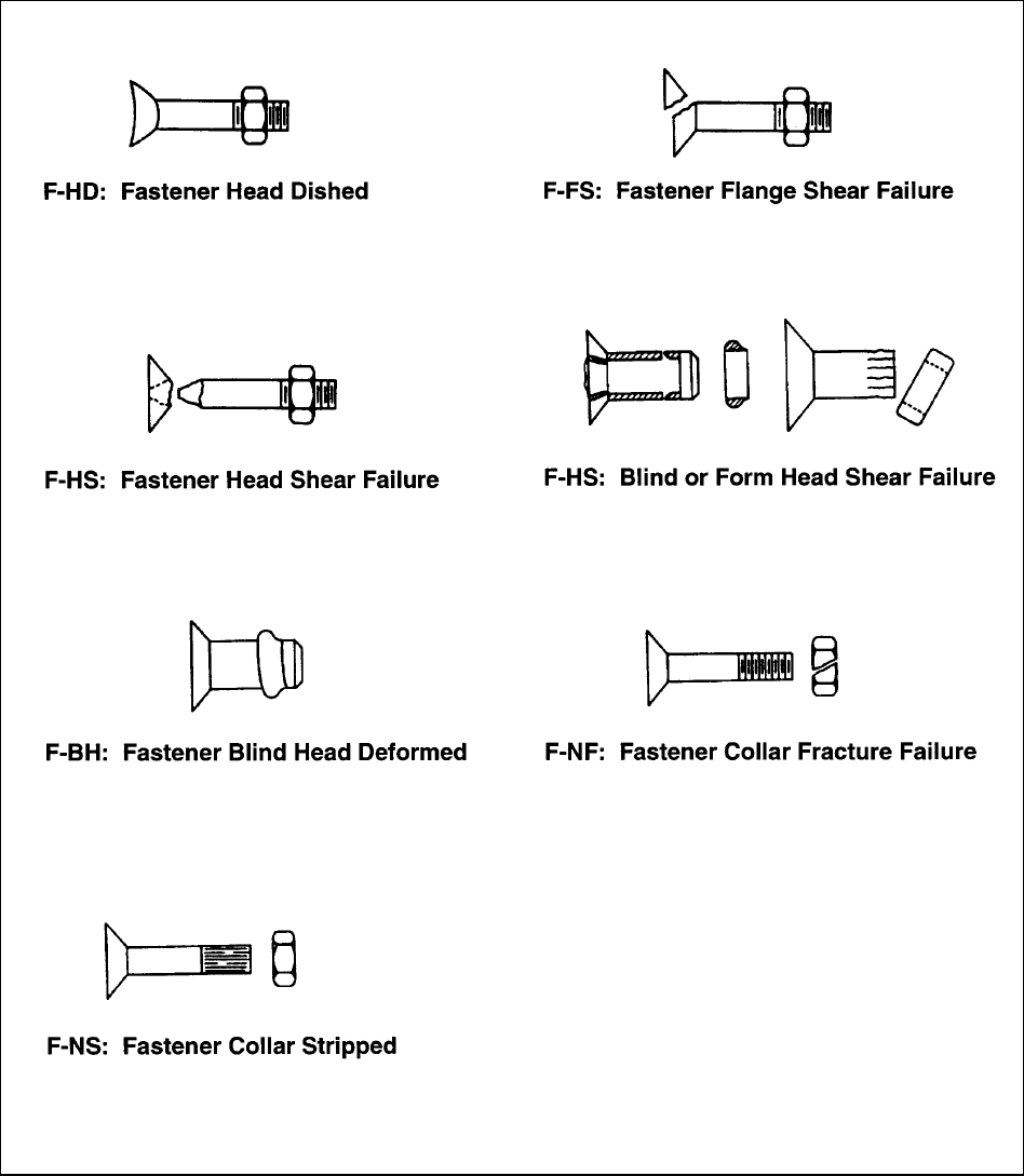
MIL-HDBK-17-1F

Volume 1, Chapter 7 Structural Element Characterization

7-29

FIGURE 7.5.2.6(c) Failure mode descriptions for mechanically fastened joints .

MIL-HDBK-17-1F

Volume 1, Chapter 7 Structural Element Characterization

7-30

FIGURE 7.5.2.6(d) Failure mode descriptions for mechanically fastened joints.

7.5.3 Bearing/by-pass evaluation

7.5.3.1 Overview and rationale

Designs of composite structure containing bolted joints in which the load transfer is greater than 20%

of the total load at an individual bolt may require test substantiation. The purpose of this section is to pro-

vide guidance on how to obtain these data. Specifically, this section describes specimen geometries, test

procedures, and test matrices to sufficiently define experimental lines AC and EC' in Figure 7.5.1.3 to

B-basis significance for the variability and environmental dependence of the material is known a priori.

Analytical procedures, e.g., see Reference 7.5.3.1, are being developed to reduce testing require-

ments. Progress has been made in the net tension/by-pass quadrant (line AC) for the failure mode char-

acterized as net tension. For this failure mode, a good correlation was obtained using linear interaction

for combined bearing/by-pass loading.

MIL-HDBK-17-1F

Volume 1, Chapter 7 Structural Element Characterization

7-31

7.5.3.2 Specimen design and testing

Various specimens and text fixtures have been utilized by the aerospace industry to obtain bear-

ing/by-pass strengths. All can be classified into three general categories: (1) passive, (2) independent

bolt load, and (3) coupled bolt load/by-pass load. In the passive method, load is transferred through the

bolt into an additional strap, as shown in Figure 7.5.3.2(a). The magnitude of the transferred load, and

hence the bearing/by-pass ratio, is thus a function of metal strip stiffness and the details of bolt installa-

tion. Without a significant amount of strain gauging, it is difficult to establish how much bearing load will

be transferred. This method/specimen is not recommended without experimental verification of load

transfer parameters. Because of geometrical limitations, this method is most applicable with low load

transfer usually not greater than 40%, which may not be where significant interaction effects occur. The

major advantage of the passive method is that it does not need special fixturing. The testing itself is

equivalent to a standard tension or in-plane stabilized compression test.

FIGURE 7.5.3.2(a) Passive by-pass/bearing specimen (single shear).

In the coupled bolt load/by-pass load method, the bolt is loaded by mechanical linkages attached to

the test machine (Figure 7.5.3.2(b)). By locating the vertical link at different locations, different bear-

ing/by-pass ratios can be tested. This ratio will remain constant until failure during each particular test.

Because of this constraint and the complexities of test fixturing, this method is also not recommended as

the primary method of obtaining bearing/by-pass data.

The recommended test method for bearing/by-pass should load the bolt independently, with the bolt

load measured directly, so that the bearing stress can be calculated without resorting to backing out a

value from strain gage readings on joining members. Test fixtures to accomplish this require a loading

cell(s) separate from the testing machine which complicates the test procedures. Specialized test fixtur-

ing has been developed by the industry to synchronize the loading between the bolt and the specimen.

One well-documented test system has been developed by the NASA Langley Research Center (Refer-

ence 7.5.3.1). Figure 7.5.3.2(c), taken from this reference, illustrates the complexities of the fixturing.

The coupon from Reference 7.5.3.1 is shown in Figure 7.5.3.2(d), modified with an additional hole to alert

the tester if any shear-out failures occurred. It is typical of all independently loaded test systems in the

industry. It should be noted that for compressive loading, the specimen is stabilized to prevent buckling.

MIL-HDBK-17-1F

Volume 1, Chapter 7 Structural Element Characterization

7-32

FIGURE 7.5.3.2(b) Bolt bearing by-pass test fixture.

FIGURE 7.5.3.2(c) Block diagram of the combined bearing by-pass test system (Reference 7.5.3.1).

MIL-HDBK-17-1F

Volume 1, Chapter 7 Structural Element Characterization

7-33

FIGURE 7.5.3.2(d) Specimen for bearing/by-pass test.

7.5.3.3 Suggested bearing/bypass test matrix

The minimum testing requirements necessary to construct the bearing/by-pass interaction plot of Fig-

ure 7.5.1.3 for a particular polymer matrix composite material are outlined in Table 7.5.3.3. The test ma-

trix assumes that the end points (

A and E) have been or will be obtained from no bolt load notch ten-

sion/compression tests recommended in Section 7.4. It also assumes that the points

C and C

are ob-

tained from the bearing strength tests enumerated in Section 7.5.2 for single shear and Section 7.2.4 for

double shear. As no environmental tests other than that at room temperature have been specified in Ta-

ble 7.5.3.3, the environmental effects on the bearing/by-pass strength are to be deduced from the interac-

tion curves' endpoints. The laminate called out are the same as in Section 7.4.2 and 7.43. For complete-

ness, the laminate lay-ups should be as follows: [+45/0/-45/(±45)

/90]

for 10/80/10, [+45/0/-45/90]

for

25/50/25, and [+45/0/-45/90/0

/+45/0]

for 50/40/10.

The test specimen and procedures to fulfill the test requirements of Table 7.5.3.3 should use an indi-

vidually loaded bolt method such as described in Reference 7.5.3.1 and shown in Figures 7.5.3.2(c) and

(d), or similar. The test matrix can be applied to either a single shear or double shear joint. In the event

that both types of joints exist in the structure the test matrix should be repeated.

7.5.3.4 Data reduction

The data reduction procedures of notched tension and bearing tests are applicable to bearing/by-pass

tests. The bolt load versus displacement plot should be obtained as for the bearing test. In addition, total

of by-pass load must be recorded. Failure mode must also be described.

MIL-HDBK-17-1F

Volume 1, Chapter 7 Structural Element Characterization

7-34

TABLE 7.5.3.3 Bearing/by-pass test matrix.

Tension Compression

Lay-up Environment

(Temp/% Moist)

Bearing/By-pass ratio Bearing/By-pass ratio Total No.

of Tests

0.75 0.50 0.75 0.50

10/80/10 RT/ambient 5 5 5 5 20

25/50/25 RT/ambient 5 5 5 5 20

50/40/10 RT/ambient 5 5 5 5 20

TOTAL 15 15 15 15 60

7.5.4 Shear-out strength

The shear-out strength of a material is its ability to withstand shear-out failure of the type shown in

Figure 7.5.1.2. Composite joints are usually designed to avoid this mode of failure. However, by reducing

the edge distance from the typical value of three times the fastener diameter (

3D), the bearing specimens

of Sections 7.2.4 and 7.2.5 can be induced to fail by shear-out. Thus these specimens and procedures

are used to determine the joint shear-out strength. The shear-out strength is calculated as

P/2et based

on the gross section. Definitions of

e, D, and t are described in Figure 7.5.4(a). The shear-out failure

mode in composite bolted joints can be avoided by having sufficient edge distance and interspersed

stacking sequence with adequate numbers of ±45° and 90° plies. Indeed, it is virtually impossible to cre-

ate a design limiting shear-out failure mode at a

3D edge distance without clustering together an exces-

sive number of plies of the same direction. On the other hand, in some situations, particularly in rework or

repair, short edge distances cannot be avoided. Thus the capability of laminates in shear-out must be

known, even when the laminate would not fail by shear-out at the nominal edge distance.

Because a pure bearing test specimen is used to determine the shear-out strength, misinterpretations

have occurred in reports that claim that the smaller

e/d ratios reduce the bearing strength of the joint.

While the shear lap specimens with small

e/D ratios do fail at lower joint bearing stresses than the lami-

nate bearing strength, it is because a lower joint failure has occurred in the shear-out failure mode in the

shearing surfaces, preempting the bearing mode of failure.

How the failure mode changes as a function of

e/D and laminate lay-up is illustrated in Figure

7.5.4(b). In this figure, failure test data for

e/D ratios between 1.5 and 2.5 and for different laminates are

plotted with bearing stress as the ordinate and shear-out stress as the abscissa. The plotted results show

a constant shear-out failure stress irrespective of bearing stress or

e/D ratio. For one laminate, even at an

e/D ratio of 2.5, sufficiently high joint load was reached to fail the joint by bearing failure. The data of Fig-

ure 7.5.4(b) also show a reduction in shear-out strength when the grouping of the same direction plies are

doubled from four to eight. Typical failures are shown in Figure 7.5.4(a) where a plug of material is dis-

placed parallel to the fiber direction without any crushing of fibers ahead of the bolt. As this shear-out

failure mode is a matrix failure, it is susceptible to degradation with environment.

MIL-HDBK-17-1F

Volume 1, Chapter 7 Structural Element Characterization

7-35

FIGURE 7.5.4(a) Shear-out failure mode.

Yet other data, for laminates with fifty percent or more of concentrated plies in the bearing load direc-

tion show shear-out failures at the same load irrespective of whether the edge distance (

e) is 2D or 8D.

So additional edge distance alone cannot be relied upon to enhance shear-out resistance of highly ortho-

tropic laminates. To avoid shear-out failure, one must avoid large concentrations of same direction plies.

The conclusion is that the shear-out strength is more dependent on the laminate and stacking order than

on the edge distance.

MIL-HDBK-17-1F

Volume 1, Chapter 7 Structural Element Characterization

7-36

FIGURE 7.5.4(b) Bearing/shear-out test failure data as a function of bearing and

shear-out stresses - AS1/3501-5A, RT, ambient.

7.5.5 Fastener pull-thru strength (MIL-HDBK-17 test method)

7.5.5.1 Scope

Test procedures for determining the sheet pull-thru characteristics of mechanically fastened compos-

ite joints are described in this section. Sheet pull-thru is defined as the load level at which two composite

plates attached by a mechanical fastener can no longer support an increase in load when the plates are

pulled apart perpendicular to the plates’ plane. Two methods are suggested; one method, an adaptation

of MIL-STD-1312 Test 8 for Tensile Strength (recently being adopted by AIA Standards Committee as

NAS M1312), is described in detail and for the purposes of this handbook will be called Procedure A. This

method is suitable for screening and fastener development purposes. The second method, Procedure B,

is suitable to establish design values, but as this test is more configuration dependent only a sketch of

possible testing configuration is provided. Both methods can be utilized to perform comparative evalua-

tions (with baseline fasteners having established usage) of the candidate fasteners/fastener system de-

signs. It is understood that the specimens described herein may not be representative of actual joints

which might contain one or more free edges adjacent to the fastener or contain multi-fasteners that

change the actual boundary conditions.

7.5.5.2 Summary of test methods

Both procedures use a flat square specimen with a constant rectangular cross-section. A centrally

located hole is used to install a fastener, see Figures 7.5.5.2(a) and (b). For Procedure A additional 4

holes are needed on the periphery of the specimen to accommodate the test fixture, Figure 7.5.5.2(c).

MIL-HDBK-17-1F

Volume 1, Chapter 7 Structural Element Characterization

7-37

Additionally, as can be seen from Figure 7.5.5.2(a), Procedure A requires two such square plates. The

two plates are joined together by the fastener, with one plate being rotated 45

° degrees with respect to

the second plate, Figure 7.5.5.2(d). These plates are pried apart by compressive loads that are transmit-

ted by the fixture of Figure 7.5.5.2(c) resulting in a tensile load on the fastener and compressive load on

the composite plate. For Procedure B one plate is connected to a yoke, Figure 7.5.5.2(e). The yoke loads

the fastener in tension creating a pull-thru force on the joint.

Both the applied load and the associated deformation are monitored in both procedures. A typical

load deflection curve is shown in Figure 7.5.5.2(f). The deflection can be measured either by the relative

cross-head displacement or by an extensometer. The first peak load observed on the load displacement

curve defines the structural failure load.

Procedure A test is easily performed as most test laboratories have the fixture shown in Figure

7.5.5.2(c). The only critical point is the correct installation of the test fastener. Additionally the composite

plates must be sufficiently stiff to transmit the compressive fixture loading without excessive plate bending

or bearing damage.

FIGURE 7.5.5.2(a) Fastener pull-thru test plate for Procedure A.

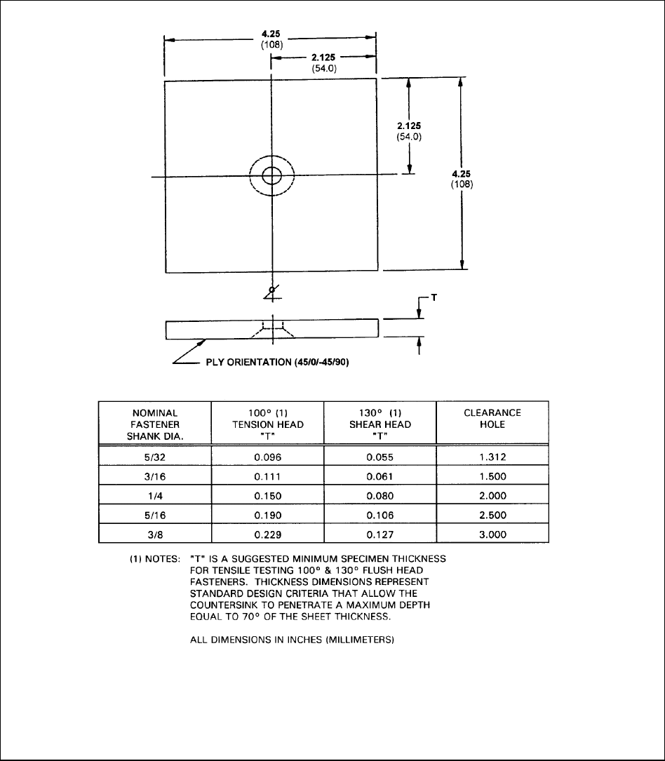
MIL-HDBK-17-1F

Volume 1, Chapter 7 Structural Element Characterization

7-38

FIGURE 7.5.5.2(b) Fastener pull-thru test plate for Procedure B.

MIL-HDBK-17-1F

Volume 1, Chapter 7 Structural Element Characterization

7-39

FIGURE 7.5.5.2(c) Fastener pull-thru test fixture for Procedure A.

FIGURE 7.5.5.2(d) Assembled test specimen for Procedure A.

MIL-HDBK-17-1F

Volume 1, Chapter 7 Structural Element Characterization

7-40

FIGURE 7.5.5.2(e) Fastener pull-thru test fixture for Procedure B.

FIGURE 7.5.5.2(f) Typical load deflection curve.

MIL-HDBK-17-1F

Volume 1, Chapter 7 Structural Element Characterization

7-41

7.5.5.3 Significance

Polymeric composites are weak in the transverse direction, therefore, the test to establish pull-thru

characteristics has acquired more significance than for metal mechanical joints. Early tests using fasten-

ers common to metal structures led to premature joint failures and resulted in development of fasteners

specific for composite applications. These fasteners have larger heads and tails to reduce transverse

compression stress on the composite laminate. Determination of the pull-thru strength of a particular

composite/fastener joint design has become a normal requirement in the design and verification of a

composite structure.

In addition to determining the pull-through strength of a particular composite plate/fastener combina-

tion, these procedures can also be utilized for evaluation of different fastener components such as

bolt/nuts, pin/collars, or washers to satisfy pull-thru strength requirements.

7.5.5.4 Apparatus

Test Machine - Testing should be conducted using a universal test machine capable of applying ten-

sion or compression load at a controlled rate per ASTM E 8 guidelines (Reference 7.5.5.4(a)). The cali-

bration system for the machine should conform to ASTM E 4, its accuracy verified every 12 months by a

method complying with ASTM E 4 (Reference 7.5.5.4(b)). The ultimate failing loads of the fasteners/joints

should be within the load range of the test machine as defined in ASTM E

Deflection Measurement – Load-deflection response should be recorded autographically. The

movement sensor should be installed to measure the relative motion between the movable cross-head

and the stationary cross-head. If a measuring device is used it should be an averaging, differential trans-

former extensometer or equivalent. It should be used in conjunction with an autographic recorder and

should have an accuracy of 0.5% of indicated joint deflection at loads equivalent to 70% of the anticipated

joint's strength and be calibrated per ASTM E 83 (Reference 7.5.5.4(c)). Load and deflection ranges

should be used that give the initial part of the load-extension curve a slope between 45° and 60°. Load

and deflection ranges and scales should be held constant for each test group (test group is defined as

specimens of the same configuration, fastener type and size and their baseline counterparts).

Test Fixture - The test fixture for the screening test should be as described in Figure 7.5.5.2(c) capa-

ble of transmitting compression loads to the test specimen. The fixtures should be parallel within 15 min-

utes of arc and capable of loading the specimen to fastener failure without experiencing local compres-

sive deformation. The test schematic for a more structure-representative test is shown in Figure

7.5.5.2(e). A load cell capable of applying a tensile load is required.

7.5.5.5 Test specimen

Test specimen configuration should be in accordance with Figure 7.5.5.2(a) for Procedure A or Figure

7.5.5.2(b) for Procedure B. For Procedure A, the composite ply lay up should be similar to Figure

7.5.5.2(d). The ply orientation provides a balanced laminate having a quasi-isotropic (25%, 50%, 25%)

distribution. The lay-up for Procedure B has been left open and should closely mimic the actual applica-

tion.

7.5.5.6 Specimen assembly

Fastener Installation – Fasteners should be installed per the manufacturer’s recommendation or

applicable process specification.

Grip Length – Fastener grip lengths should be selected to ensure full shank bearing through the total

specimen thickness. Fasteners with load bearing tails that are formed during installation and bear against

the composite test surface should be tested in both minimum and maximum grip conditions. This is be-

cause the effective bearing area may vary from one grip condition to the other.

MIL-HDBK-17-1F

Volume 1, Chapter 7 Structural Element Characterization

7-42

Fasteners with manufactured heads used in conjunction with nuts or collars that do not change shape

affecting the bearing surface being tested, should be tested in nominal grip condition.

Head Flushness – Unless otherwise specified flush head fasteners should be installed within ±.005

inches (±0.1 mm) from the composite surface.

7.5.5.7 Test matrix

A suggested test matrix to be used for fastener screening or development is shown in Table 7.5.5.7.

Procedure A test specimen (Figure 7.5.5.2(d)) is to be used in conjunction with this test matrix that repre-

sents the required testing for one fastener configuration. The testing should be performed at room tem-

perature, ambient and hot, wet conditions. The latter is defined as the highest temperature and moisture

content for the composite material (see Section 2.2.8). The test matrix is to be repeated for a different

fastener, head or tail configuration, and installation hole clearance. As used in Table 7.5.5.7, Class 1 is

reserved for interference fit, Class 2 for aircraft quality, usually +0.003 in (+0.08 mm), and Class 3 for

clearance fit.

A test matrix similar to Table 7.5.5.7 should be constructed for the Figure 7.5.5.2(e) test (Procedure

B). However, as the test is more design-oriented, fewer variables need to be tested. The replication of 5

should be maintained.

7.5.5.8 Report

The test results should be reported in terms of structural failure load, load-deflection curve, and the

observed failure mode.

7.5.6 Fastener-in-composite qualification tests

7.5.6.1 Overview

A first step in design of composite bolted joints is the identification of fasteners that are suitable for

use with composites. The data generated by tests outlined in this section will provide a realistic basis for

selection as the tests will give a good estimate of joint strength. Composites require fasteners with larger

tail footprints (than metals), especially for blind fasteners; the tests described here will interrogate this fea-

ture. After fastener selection additional test data, enumerated in Sections 7.5.2 and 7.5.6, will be needed

to design bolted joints for other laminates and failure modes that are not a function of specific fastener

characteristics.

The test requirements and methods have been extracted from Sections 7.5.2 and 7.5.6, thus details

of testing procedures can be obtained from those sections. Testing for fastener-in-composite qualification

uses only one laminate lay-up (quasi-isotropic), but more than one thickness. Also, the testing is limited to

room temperature as the environment is not a driver for fasteners as it is for composites. The test pro-

gram is based on the assumption that the plates to be joined are both composites. If the particular fas-

tener is also intended for use in metal/composite combinations, testing should be performed for that con-

figuration. The test matrices reflect two properties most affected by fastener properties: joint bearing and

pull-thru strengths. It is suggested that pull-thru tests be conducted first to determine the suitability of the

fastener for composites. Once that property is satisfactory, the more expensive bearing tests can be un-

dertaken. In aircraft industry, there is also a requirement established by aircraft manufacturers and certify-

ing agencies that 25% of bearing and pull-thru tests be tested by someone other than the manufacturer of

the fastener. For inclusion of data in the MIL-HDBK-5, the fastener must be in-use by at least one aircraft

manufacturer. For completeness, test requirements for fastener shear and tensile strengths are included

here, although these properties are independent of joining members.

MIL-HDBK-17-1F

Volume 1, Chapter 7 Structural Element Characterization

7-43

TABLE 7.5.5.7 Fastener pull-thru test matrix.

GEOMETRY

COMPOSITE

SHEET

THICKNESS

in. (mm)

LAY-UP

FASTENER

NOMINAL

SHANK DIAMETER

in. (mm)

INSTALLATION

HOLE CLASS

ENVIRONMENT

(TEMP/% MOIST)

NUMBER

TESTS

(1)

COMPOSITE

0.190 (4.83)

Head side

25/50/25

0.250 (6.35)

Class 2

RT/ambient

hot/wet

COMPOSITE

0.120 (3.05)

Tail side

25/50/25

0.250 (6.35)

Class 2

RT/ambient

hot/wet

COMPOSITE

METAL (2)

(Metal on

head side)

0.190 (4.83)

25/50/25

0.250 (6.35)

Class 3

RT/ambient

hot/wet

COMPOSITE

METAL(2)

(Metal on tail

or nut side)

0.160 (4.06)

25/50/25

0.250 (6.35)

Class 2

RT/ambient

hot/wet

Notes: (1) Each grip condition where applicable (see Section 7.2.9.4).

(2) Metal thickness can be varied to accommodate fastener grip length.

MIL-HDBK-17-1F

Volume 1, Chapter 7 Structural Element Characterization

7-44

Fasteners for use with carbon fiber composites should be titanium, A286 CRES or Monel to reduce

the potential for galvanic corrosion. In some applications, particularly space applications, galvanic corro-

sion is not a problem. This limitation does not apply to aramid or fiberglass composites.

The data generated by the test program presented here will not be sufficient by itself to qualify a fas-

tener for use in aircraft structures. Fatigue testing, manufacturing tolerances studies (grip lengths, seating

angles, hole diameters) are the other criteria that have to be satisfied to complete fastener qualification

requirements.

7.5.6.2 Fastener shear tests

These tests are conducted using steel plates per MIL-STD-1312, Test 13 for double shear and Test

20 for single shear (Reference 7.5.2.3.2). Evidence of previous valid qualification tests could be accepted

here.

7.5.6.3 Fastener tension tests

These tests are conducted in steel plates per MIL-STD-1312, Test 8 (Reference 7.5.2.3.2). Evidence

of previous valid qualification tests could be accepted here.

7.5.6.4 Fastener Pull-thru tests

Test specimen configuration to determine pull-thru strength should be in accordance with Figures

7.5.5.2(a), (b), and (c). The test procedures are given in Section 7.5.5. The test matrix, Table 7.5.6.4, re-

quires testing for three different diameters representative of the applicability of the fastener. One diameter

should be 0.25 in. This may require adjustments in laminate thickness; however, the laminate lay-up must

be maintained as (45/0/-45/90)

. The test matrix is to be repeated for each fastener under consideration.

TABLE 7.5.6.4 Fastener qualification pull-thru test matrix

Geometry

Composite

Sheet Thickness

in. (mm)

Lay-Up

Fastener Nominal

Shank Diameter

in. (mm)

Number of

Tests

Composite to

Composite

0.190 (4.83)

Head Side

25/50/25 0.25 (6.4) 5

0.120 (4.83)

Tail Side

25/50/25 0.25 (6.4) 5

Head Side

25/50/25

Tail Side

25/50/25

Head Side

25/50/25

Tail Side

25/50/25

Notes:

All tests to be performed at RT/ambient and with installation hole Class 2.

Each grip condition where applicable (see Section 7.5.5.4).

May be different for other diameters.

MIL-HDBK-17-1F

Volume 1, Chapter 7 Structural Element Characterization

7-45

7.5.6.5 Bearing tests

The composite-to-composite two bolt bearing specimen geometry shown in Figure 7.5.2.3.2(b) is

suggested. This single shear configuration is more representative of multi-fastener joints found in the in-

dustry. With an acceptable fastener, composite bearing failure should be achieved, although secondary

fastener rotation about its longitudinal axis may be evident. The test matrix for fastener qualification is

shown in Table 7.5.6.5. Three different thicknesses of one lay-up (45/0/-45/90)

and three fastener di-

ameters are suggested. One diameter should be 0.25 in. (6.35 mm) and the other two reflecting the range

of available fastener sizes. Selection of additional thicknesses of the composite members should stay

within these guidelines to assure maximum usefulness of data: (1)

0.8<D/t<2 and (2) countersink depth

should not exceed 0.67 of total laminate thickness. The goal of the tests is to obtain a family of three

curves of bearing stress versus

D/t ratio for each diameter tested. There should be 15 data tests for each

diameter. The test matrix is to be repeated for each fastener under consideration.

TABLE 7.5.6.5 Fastener qualification bearing test matrix

Geometry

Thickness

in. (mm)

Lay-Up

Bolt Diameter

in. (mm)

Number

of Tests

Composite

0.2 (5)

25/50/25

0.25 (6.4)

Composite

25/50/25

0.25 (6.4)

Composite

25/50/25

0.25 (6.4)

Note:

All tests are to be performed at RT, ambient.

7.5.6.6 Data presentation

Data presentation should follow the guidelines of Volume 2, Section 1.4.2. Additionally, bearing data

should be presented as plots of bearing strength vs.

D/t for each diameter tested.

7.5.7 Bearing/mechanical joint test methods for MIL-HDBK-17 data submittal

For bearing strength, test data obtained from ASTM D 5961 are publishable in MIL-HDBK-17 either as

double shear values, Procedure A, or single shear values, Procedure B. For design values the two bolt

specimen is more representative of actual joints.

No bearing/by-pass method is recommended, however, a test method that measures the by-pass

load directly will produce acceptable data for MIL-HDBK-17.

Shear-out strength values are acceptable for MIL-HDBK if obtained from the bearing tests of ASTM

D 5961. The failure mode for these tests must be distinctly observed as shear-out and not bearing.

Pull-thru strength test data from Procedure A of Section 7.5.5 is acceptable for inclusion in MIL-

HDBK-17. Data obtained using Procedure B, although acceptable for establishing design values, may be

very configuration dependent and hence not usable for others.

MIL-HDBK-17-1F

Volume 1, Chapter 7 Structural Element Characterization

7-46

7.6 BONDED JOINT TESTS

7.6.1 Overview

In principle, bonded joints are structurally more efficient than those that are mechanically fastened.

Bonded joints eliminate hole drilling for fastener installation resulting in a structure without notches that

cause stress concentrations. Composite structures can have bonded joints fabricated by three different

processes: secondary bonding, co-bonding, and co-curing. Secondary bonding uses a layer of adhesive

to bond two pre-cured composite parts. Thus, this type is most similar to metal bonded joints in structural

behavior and fabrication method. Co-curing is a process wherein two parts are simultaneously cured.

The interface between the two parts may or may not have an adhesive layer. In the co-bonding process

one of the detail parts is pre-cured with the mating part being cured simultaneously with the adhesive.

Surface preparation is a critical step in any bonded joints and must be clearly defined before any bonding

is performed. This is particularly important in secondary and co-bonding processes. More detail on

bonded joint fabrication is given in Volume 3, Section 2.9.

The type of bonded joints addressed in this section are secondarily bonded and co-bonded. For

these types of joints, knowledge of mechanical properties, particularly stiffness of the adhesive, is a de-

sign imperative. Well designed adhesive joints in aircraft structures are not critical in the adhesive layer

but in the adherends, whether they be metal or composites, but this does not obviate the need to know

the strength capability of the adhesive in shear and tension. The composite adherends are in most in-

stances well constructed laminates with sufficient number of plies in the principal load directions ensuring

that the failure mode is fiber dominated. The properly selected adhesives are formulated to be much

more ductile than the resins used as matrices in composites as they are not required to provide support to

fibers, particularly under compressive loading, thus steering the joint failure to the adherends. The fibers

also constrain the resin so that the behavior of the matrix is also more brittle than the resin by itself. This

may shift the composite bonded joint failure to a transverse, through the thickness, tensile failure of the

composite laminate.

Two distinct type of tests are needed to characterize the behavior of a bonded joint and obtain suffi-

cient mechanical data to perform structural analysis. It is assumed that the mechanical properties of the

composite adherends are known. For simplicity and standardization goals, the tests to determine adhe-

sive properties make use of metal adherends. The results of these tests provide properties of adhesive

for design and analysis, comparative data, surface preparation effectiveness, but in no way represent the

strength of a composite structural bonded joint. This is obtained by testing specimen configurations with

composite and/or honeycomb adherends that are more application representative. Both types of testing

are discussed in the sections that follow.

7.6.2 Adhesive characterization tests

Adhesive strength and stiffness data is required if successful bonded joints are to be designed. As

adhesive behavior is elastic-plastic, it is not sufficient to characterize the adhesive by ultimate strength

and initial tangent modulus. The data that are needed include stress-strain curves in shear and tension at

the service temperature and humidity environments.

The test methods that are currently favored by the industry to obtain these data are the thick adher-

end test for the shear properties that was pioneered by Krieger (Reference 7.6.2 (a) and 7.6.2 (b)) and

resulted in ASTM D 5656, and the ASTM D 2095 (Reference 7.6.2 (c)) test for the tensile strength by

means of bar and rod specimen. None of the tests are completely satisfactory for various reasons. How-

ever, as they have gained widespread usage, it is deemed useful to have them referenced in this chapter.

Moisture conditioning of adhesive specimens to equilibrium (uniform moisture content of the entire

bondline) before wet testing requires prohibitive duration times - several years. This is because of low

values of moisture diffusivity of common adhesives and the use of test specimens with moisture impervi-

ous metal adherends for which water can only enter the adhesive through exposed bondline edges. For-

MIL-HDBK-17-1F

Volume 1, Chapter 7 Structural Element Characterization

7-47

tunately, adhesive failures usually initiate at bond edges, due either to shear stress peaking or to peel

(tensile) stresses. Thus, as long as a reasonable depth of adhesive near the edges has approached the

desired equilibrium moisture level, test results will be representative of a fully equilibrated bondline. The

common practice of exposing test specimens to the required relative humidity at reasonably high tem-

peratures (160 to 180°F (71-82°C) for epoxies) for 1000 hours (42 days) achieves this goal. An alterna-

tive method to determine the effect of absorbed moisture on adhesives is to use cast adhesive neat resin

specimens and perform tension and compression tests. As in this case the entire specimen is exposed,

the times to reach equilibrium are significantly less.

7.6.2.1 Shear tests

7.6.2.1.1 ASTM D 5656 (thick adherend specimen)

This test method uses the KGR-1 extensometer that is attached to a specimen of geometry shown in

Figure 7.6.2.1.1(a). Typical data obtained by this test is shown in Figure 7.6.2.1.1(b) for one adhesive at

different temperatures. Because of KGR-1 design and use of aluminum adherends, the test method is

limited to 300°F (150°C). For higher temperature applications titanium adherends have been used to in-

crease the usable temperature of the method.

FIGURE 7.6.2.1.1(a) Thick adherend specimen (Figure 2 from D 5656).

MIL-HDBK-17-1F

Volume 1, Chapter 7 Structural Element Characterization

7-48

FIGURE 7.6.2.1.1(b) Shear stress-strain response of FM 300 K adhesive at different

temperatures in °F.

How to interpret the shear stress-strain curves of Figure 7.6.2.1.1(b) in terms of adhesive shear

modulus has been a subject of numerous papers. Krieger in Reference 7.6.2(a) states that only a small

correction for adherend deformation is needed to obtain adhesive properties and that by characterizing

the stress-strain curve using three points, all the necessary information for design of bonded joints with

the particular adhesive is determined. These three points are shown in Figure 7.6.2.1.1(c). A more ex-

tensive analysis of the test method and the associated measurement device was performed by Kassapo-

glou and Adelmann in Reference 7.6.2.1.1(a). They found the method to be reasonably accurate for soft

adhesives, but suggest some improvements for other situations. However, their conclusions are limited to

the elastic range and the method is considered quite adequate for measuring stress-strain response in

the plastic (large deformation) region. Reference 7.6.2.1.1(b), using Moire' fringe interferometry, validated

Krieger measurements, but found the method susceptible to loading eccentricities which causes early

failure and large scatter in modulus measurement. Reference 7.6.2.1.1(b) also suggested using a strain

gage at the geometrical center of the bondline instead of the KGR-extensometer if the data of interest is

the initial tangent modulus.

For bonded joint stress analysis, the test stress-strain curves of Figure 7.6.2.1.1(b) are sometimes

further simplified to a perfect elastic-plastic material response, as described in Reference 7.6.2.1.1(c).

Thus, the stress-strain data as obtained by the thick adherend test, although not 100% correct, is of suffi-

cient accuracy for the current design and analysis methodology.

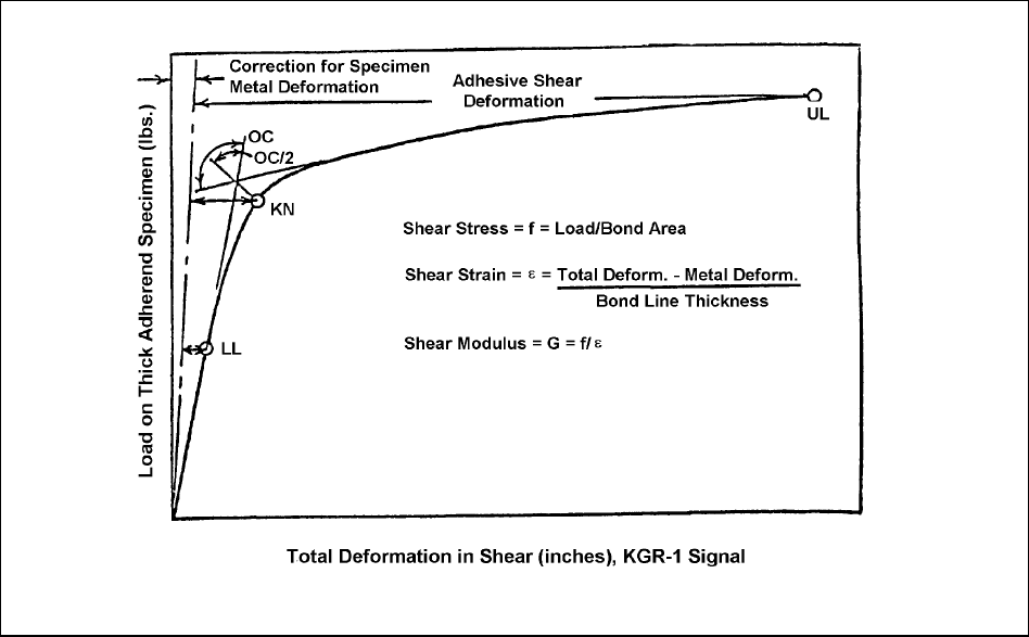
MIL-HDBK-17-1F

Volume 1, Chapter 7 Structural Element Characterization

7-49

FIGURE 7.6.2.1.1(c) Load deformation curve with critical points to determine elastic-plastic response.

7.6.2.1.2 ASTM E 229 (tubular specimen)

An alternate method to obtain shear strength and stiffness is by use of a tubular specimen loaded in

torsion. The basis of the test is a narrow, annular ring of adhesive subjected to uniform shear loads

around the circumference. Because the thickness of the tube is small compared to its radius, the shear

stress across it is considered constant. Although the test provides pure shear distribution, the test appa-

ratus is complex and specialized testing know-how is required which have led to the disuse of this test

method. A test method utilizing the tubular specimen is the ASTM E 229 Standard Test Method (Refer-

ence 7.6.2.1.2). It uses narrow but large diameter adherend tubes and measures angle of twist by an

Amsler Mirror Extensometer. Details of the test are described in the standard.

7.6.2.1.3 ASTM D 1002 (thin single lap spec. - QA test only)

The single lap shear test described in the ASTM D 1002 is a test that is widely used for comparative

evaluation of the adhesive and for qualification and incoming inspection purposes. The test is also useful

to evaluate surface preparation procedures as this test uses metal adherends. The main attribute of this

test is that it is easy to fabricate and test.

Limitations of this test are

Shear Strength – The maximum shear stress obtained from this test (maximum load divided by

bond area) has no relation to the adhesive shear strength. The stress field in the adhesive has a

large component of peel stress that contributes to the specimen failure. The apparent shear

strength will also be a function of the adherend modulus and its thickness. Because the apparent

shear strength will vary with adherend modulus and thickness, for comparative purposes, the

specimen configuration should be kept constant. ASTM D 4896 should be consulted for interpre-

tation of test results.

MIL-HDBK-17-1F

Volume 1, Chapter 7 Structural Element Characterization

7-50

Shear Stiffness – The test cannot measure adhesive stiffness because of large bending inherent

in the specimen.

Joint Realism – Because the adherends are metal, the test cannot simulate failure modes of a

composite to composite bonded joint. Surface preparation and adhesion are completely unrepre-

sentative of a composite to composite bonded joint. Furthermore, as the process to fabricate

composite bonded joint will be quite different to the fabrication of this metal to metal lap joint, this

specimen cannot be used for in-process control.

To address the problem of joint realism, the ASTM D 1002 has been modified to admit composite adher-

ends. ASTM D 3163 is the resulting standard. This standard, however, has all the other limitations of

ASTM D 1002. When using this standard, in addition to thickness, the lay-up of the composite material

must approximate the joint laminate as the apparent shear strength will vary with lay-up. For composite

applications, the use of this standard is preferable if the properties of the adhesive/adherend interface

characterization are of interest. If the primary purpose is adhesive characterization, then ASTM D 5656

should be used.

7.6.2.2 Tension tests

7.6.2.2.1 ASTM D 2095

Tensile strength of the adhesive can be obtained by the ASTM D 2095 method, Figure 7.6.2.2.1 (Ref-

erence 7.6.2(c)). Either bar or a rod specimen can be used in this test method. The design of the speci-

mens and specimen preparation is described in ASTM Recommended Practice D 2094 (Reference

7.6.2.2.1(a)). The tensile strengths obtained by this test method should be used with caution as the test

specimen is susceptible to peel initiated failure at the specimen edges. The adhesive failure strength can

be used in an approximate peel analysis as proposed in Reference 7.6.2.2.1(b). As good bonded joint

design practice minimizes peel stresses, the exact knowledge of tensile strength capability is not that criti-

cal.

An independent measurement of the Young's modulus of the adhesive is needed as the adhesive

often does not obey laws of isotropic materials and can not be obtained from shear modulus measure-

ment, i.e.,

(

)

7.6.2.3 Fracture mechanics properties

Another approach to determining the behavior of bonded joints is to use fracture mechanics. This

analysis and failure criteria requires testing to obtain critical strain energy release rates in modes I and II.

The tests to be performed are described in Section 6.8.6.

7.6.2.4 Suggested adhesive characterization test matrix

Tests for adhesive properties should be performed at room temperature, ambient conditions, and at

low and high usage temperature extremes as discussed in Section 2.2.8. The replication should be a

minimum of five at each test condition.

7.6.3 Bonded joint characterization tests

Tests of bonded joint configurations representative of actual joints must be tested to validate the

structural integrity of the joint. As these specimens quickly become point design oriented, it is difficult to

standardize. Thus the discussion will be limited to the simplest specimens which contain the important

parameters of the bonded composite joint: geometry, composite laminates and/or metal adherends, ad-

hesive, fabrication process, and quality control procedures.

MIL-HDBK-17-1F

Volume 1, Chapter 7 Structural Element Characterization

7-51

FIGURE 7.6.2.2.1 Test specimens and attachment fixtures.

7.6.3.1 Honeycomb to face sheet flatwise tension test (ASTM C 297)

For honeycomb construction there is a need to determine the strength of the bond between the core

and the facings of an assembled sandwich panel. ASTM C 297 is the test most commonly used by the

industry (Reference 7.6.3.1). The specimen and test assembly is shown in Figure 7.6.3.1. The specimen

size is usually 2 by 2 in., but can be round. It is important to use the same processing to fabricate the

specimen as for the actual component in order to have meaningful results. This test does not determine

adhesive tensile strength, but does give an indication how well the adhesive wets the walls of the honey-

comb. The failure mode should be recorded, as for some configurations the bond has a higher tensile

strength than the honeycomb itself. In most applications the honeycomb-to-facesheet bond has higher

strength than the core, but for this test, to induce bond failures higher strength core should be used. The

main difficulties encountered with this specimen are bonding of the fixture to the face sheet, especially at

elevated, wet environmental conditions, and maintaining parallelism between the fixtures and the speci-

men.

MIL-HDBK-17-1F

Volume 1, Chapter 7 Structural Element Characterization

7-52

FIGURE 7.6.3.1 Flatwise tensile loading fixture and specimen.

7.6.3.2 Skin to stiffener bond tests

To assess the strength of skin-to-stiffener bonded joints in situations where out-of-plane loads are

being developed, i.e., fuel pressure, post-buckling, fairly simple tests are being used in the industry. Al-

though these tests cannot completely represent the behavior of the actual structure, they provide design

data and early assessment of the adequacy of selected materials and geometry before commitment to

large component validation tests. The maximum benefits from these tests are obtained when the speci-

mens represent as closely as possible the geometry and fabrication processes of the simulated compo-

nent. The schematics of two such tests are presented here. The "T" pull-off test shown in Figure

7.6.3.2(a) is similar to the ASTM C-297 except that only one block is needed. Because the bending of the

skin and stiffener flanges are suppressed by the rigid loading block, the disbond failure will generally oc-

cur in the heel of the stiffener and not at the flange ends. This is a serious deficiency of the specimen, if

in component tests the failure is at flange ends. The location of the failure is strongly dependent on the

ratio of stiffener/skin stiffness; the lower the ratio, the more useful is the test.

Using rollers to resist the pull-off load instead of the rigid block, Figure 7.6.3.2(b), can be a better

method if the skin is more flexible. There is the problem how far apart to place the rollers to match the

skin displacement. The specimen in Figure 7.6.3.2(b) can be used to apply a moment to the bonded joint.

This is represented by

P1 loads and R1 reactions in Figure 7.6.3.2(b). Post-buckling of shear panels in-

troduces significant twisting moments in the interface and the capability of the joint against them must be

determined as part the structural analysis.

MIL-HDBK-17-1F

Volume 1, Chapter 7 Structural Element Characterization

7-53

FIGURE 7.6.3.2(a) “T” pull-off specimen.

FIGURE 7.6.3.2(b) “T” twist-off specimen.

MIL-HDBK-17-1F

Volume 1, Chapter 7 Structural Element Characterization

7-54

7.6.3.3 Double overlap joint tests

Double overlap specimens range between single step type to ones containing many steps and are

usually loaded in tension. The complexity being dependent on what type of data is to be obtained or the

structural application. An example of a specimen derived from ASTM D 3528 - 92 (Reference 7.6.3.3) is

shown in Figure 7.6.3.3(a). This test specimen is useful for determining adhesive shear strength as the

double shear configuration reduces peel stresses. This configuration is not usually used in design, as the

load transfer capability can be increased significantly by tapering the outside adherends.

For higher load transfer, double lap joints will contain many steps. To validate such a joint, specimens

of a type shown in Figure 7.6.3.3(b) have been used. These type of specimens are quite expensive to

fabricate and hence are not replicated in large numbers. As these specimens are to represent a particular

design, care must be taken that the specimen is manufactured using the same processes as the actual

joint. Another example of a joint verification specimen is shown in Figures 7.6.3.3(c) and (d). It represents

a chordwise connection between a composite skin and a titanium spar and is a double lap two-step joint.

The multi-step joint specimen could be converted to scarf joint specimen if that was the actual design.

FIGURE 7.6.3.3(a) Geometry and materials of the double-lap test specimens.

MIL-HDBK-17-1F

Volume 1, Chapter 7 Structural Element Characterization

7-55

FIGURE 7.6.3.3(b) Step lap joint specimen example.

FIGURE 7.6.3.3(c) Specimen configuration.

MIL-HDBK-17-1F

Volume 1, Chapter 7 Structural Element Characterization

7-56

FIGURE 7.6.3.3(d) Concept A detail, two-side stepped joint.

7.6.3.4 Single overlap joint tests

Single overlap specimens are similar to those described in the above section. However, because sin-

gle overlap specimens induce additional peel stresses due to bending, the length of the joint must be

longer to minimize that effect. This effectively eliminates usefulness of single step specimens to deter-

mine strength property of realistic joints. Single step single overlap joints, however, are used for compari-

son between different adhesives and for quality control. Two different approaches to minimize peel

stresses in single lap test specimen are described in this section. The ASTM D 3165 method minimizes

peel by keeping the load line in the adhesive layer similarly to the single shear bearing tests of ASTM D

5961, Procedure B. The second approach, exemplified by European Aircraft Industry Standard prEN

6066, reduces peel stresses by easing the load into the joint by scarfing or by multiple small steps.

7.6.3.4.1 ASTM D 3165

This method measures comparative shear strength of adhesive joint when tested using single lap

specimen of Figure 7.6.3.4.1. This specimen is used widely in the industry as an alternative to the ASTM

D 1002 or ASTM D 3163 as it reduces the peel stresses in the lap while retaining the interface realism of

a composite bonded joint. All the limitations enumerated for ASTM D 1002 in Section 7.6.2.1.3 are appli-

cable here. For composites, there is an additional difficulty in fabricating this type of specimen. The usual

procedure of machining the notch can be substituted by placing a spacer in the notch area and laying-up

separate laminates. Both manufacturing methods need trained composite engineers and mechanics to

establish a manufacturing process that will result in useful specimens.

MIL-HDBK-17-1F

Volume 1, Chapter 7 Structural Element Characterization

7-57

FIGURE 7.6.3.4.1 Form and dimensions of test specimens.

7.6.3.4.2 European Aircraft Industry Standard EN 6066

A 1 in. (25 mm) wide multi-step or scarfed specimen has been developed for bonded joint characteri-

zation. This specimen, shown in Figure 7.6.3.4.2(a) is referenced in a preliminary European Aircraft In-

dustry Standard EN 6066 (Reference 7.6.3.4.2). This standard also defines types of failures that are pos-

sible with such a specimen, Figure 7.6.3.4.2 (b). This testing standard has been called out for obtaining

qualification data for a wet lay-up repair material.

MIL-HDBK-17-1F

Volume 1, Chapter 7 Structural Element Characterization

7-58

FIGURE 7.6.3.4.2(a) Scarfed and stepped joint specimens.

MIL-HDBK-17-1F

Volume 1, Chapter 7 Structural Element Characterization

7-59

FIGURE 7.6.3.4.2(b) Determination of failure modes and dimensions for joint specimens

(Reference 7.6.3.4.2).

7.6.3.4.3 Other examples

Two-step and scarfed verification specimens are shown in Figures 7.6.3.4.3(a) and (b) for the same

spar to skin joint shown in Figure 7.6.3.3.3(b). Such specimen should be developed to validate any major

joint design.

MIL-HDBK-17-1F

Volume 1, Chapter 7 Structural Element Characterization

7-60

FIGURE 7.6.3.4.3(a) Concept B detail, one-side stepped joint.

FIGURE 7.6.3.4.3(b) Concept C detail, scarf joint.

7.7 DAMAGE CHARACTERIZATION

7.7.1 Overview

Damage characterization is a key parameter in the use of composite materials in aerospace applica-

tions. Unlike traditional metallic materials, composites vary in strength depending on direction and lay-up.

They can also be relatively brittle. Interlaminar tensile and shear strengths are especially low compared

to isotropic metallic materials. Damage such as internal delaminations may not even be visually appar-

ent. This combination of attributes makes consideration of damage characterization a key factor in the

use of composite materials. Approaches for consideration of damage in design and certification are found

in Section 5.0 of Volume 3.

MIL-HDBK-17-1F

Volume 1, Chapter 7 Structural Element Characterization

7-61

Damage characterization can be divided into two issues, the resistance of a material to damage from

impact (damage resistance), and the ability of a material or structure to perform safely after damage

(damage tolerance). Damage can occur while handling during the manufacturing process, while in use or

during maintenance procedures. This damage can be the result of manufacturing defects, foreign body

impacts such as rocks or ice, or tool drops. This section will outline impact and indentation tests that are

commonly performed to evaluate the damage resistance and tolerance of candidate materials. Crack

growth, micro-cracking and fatigue tests are discussed elsewhere in this handbook.

7.7.2 Damage resistance

Damage resistance of a material is commonly considered to be the resistance of the material to im-

pact damage in aerospace applications. Impacts may arise from dropped tools, foreign objects such as

rocks on runways, from hail and ice, and from ballistics. Impact testing is commonly used to screen mate-

rials for damage resistance and tolerance and as a part of larger sub-element and element tests per-

formed during certification.

Simulation of all these conditions may require testing at differing energy levels, velocities, impactor

geometries, and support conditions.

7.7.2.1 Falling weight impact

Another common method for investigating impact resistance is the falling weight test. This type of

impact is included as a portion of the Compression After Impact (CAI) testing discussed in Section 7.7.3.

Generally, a flat panel is impacted normal to its surface. Commonly, 0.5 inch to 1 inch (12.7 to 25.4 mm)

diameter hemispherical tups are used. Quasi-isotropic laminates approximately 0.2 to 0.4 inch (5.08 to

10.16 mm) thick are often used to screen materials for aircraft structural applications. The energy of the

weight at impact is given by the classical equation.

E = ½ mv

=mgh

E = energy

m = mass

v = velocity

g = gravitational constant of 9.8 m/sec

or 32 ft/sec

h = drop height

Since

g is constant, energy levels for the falling weight test are generally given in foot-pounds or foot-

pounds per inch of thickness. With variations of velocity of the falling weight, the damage may vary with

even constant energy. This phenomenon is related to the type of damage, the rate it propagates in the

specimen and the deformation of the specimen during impact.

The falling weight used for CAI testing is generally dropped from a few feet, with a mass of 10 to 20

pounds, and is considered a low velocity impact. Low velocity tests such as a falling weight do not ade-

quately simulate ballistic damage. Occasionally investigators may accelerate the drop with elastic cords to

gain a somewhat higher velocity. If very low velocity impacts are to be studied, a long fulcrum pendulum

may be used to impact the specimen with a much higher mass.

Following the impact, an assessment of the damage must be performed. Criteria for damage as-

sessment may include measurement of the visually apparent damage area, measurement of dent depth,

and non-destructive evaluation, such as C-Scan, for the internal damage area. Following this assess-

ment, additional mechanical tests such as CAI or fatigue may be performed.

MIL-HDBK-17-1F

Volume 1, Chapter 7 Structural Element Characterization

7-62

Sources of Experimental Error

1. The velocity may be slower than predicted due to friction on the guide rails/tube. To ensure accuracy

the actual weight velocity should be measured just prior to impact.

2. Steps should be taken so the weight does not bounce and impact the specimen more than once.

3. The amount of damage will be dependent on the specimen support conditions, such as clamping ar-

rangements. These must be reproduced very carefully. The overall stiffness of the base of the ma-

chine and even the flooring under the impactor may influence the test results.

7.7.2.2 Izod and charpy impact

Izod and Charpy impact are common classical tests performed on plastic and metallic materials.

These tests are described in ASTM D 256. Within the ASTM standard, five procedures are given. The

Izod test is discussed in procedures A, C and D of the standard and uses a notched rectangular bar 2.5”

X 0.5” X 0.25” to 0.5” (6.35 cm x 1.27 cm x .635 cm x 1.27 cm) thick. One end of the specimen is held in

a vise as a vertical cantilever and impacted on the same face as the notch, at a fixed distance above the

notch and vise, by a weighted pendulum. The energy lost by the pendulum during impact is measured

and the Izod impact strength is calculated. Procedure C contains a correction factor for the energy re-

quired to toss the broken specimen part. This factor is considered significant for materials with Izod im-

pact strengths less than 0.5 ft-lbsf/inch of notch.

The Charpy test was formerly discussed in Procedure B, but has been removed as of 1997 and has

been issued as a new standard, ASTM D 6110. It also uses a notched rectangular bar 2.5” X 0.5” X 0.25”

to 0.5” (6.35 cm x 1.27 cm x .635 cm x 1.27 cm) thick. In this test the specimen is supported as a hori-

zontal simple beam and is broken by the pendulum with the impact site halfway between the supports and

directly opposite the notch.

Procedure D is a variation on the Izod tests, but with differing notch radii. This can give an indication

of the notch sensitivity of the material.

Procedure E is a reversed-notched Izod test. It is similar to Procedure A except the specimen is im-

pacted on the face opposite the notch. This procedure gives an indication of the unnotched impact

strength of the plastic.

None of the tests in ASTM D 256 are generally appropriate for continuously reinforced composite

materials, and data from these tests will not be accepted into MIL-HDBK-17.

7.7.2.3 Quasi-static indentation

Quasi-static indentation tests may be performed by supporting a flat panel in a frame and indenting

the center of the panel with a tup attached to a universal-testing machine. This method is described in

ASTM D 6264. The most common test specimen is a 6” X 6” (15.24 x 15.24 cm) quasi-isotropic laminate,

approximately 0.17” (4.32 mm) thick. The specimen may be simply supported on a frame with a 5-inch

diameter cutout, or on a solid, flat, rigid support. Load and cross-head displacement are measured during

the test and the resulting curve is reported. A predefined level of damage or cross-head displacement is

used to define where to take data during the test and where to stop the test in the case of the rigidly sup-

ported configuration. In the case of the simple support configuration, the maximum indentation force is

also reported. Dent depth and damage are evaluated after the specimen is unloaded.

7.7.2.4 Other damage resistance tolerance tests

Other impact tests are often included at higher levels of the building block approach. These may in-

clude ballistic impact, ice/hail simulation, bird strike simulation and other program specific tests. These

MIL-HDBK-17-1F

Volume 1, Chapter 7 Structural Element Characterization

7-63

are often accomplished through use of an air gun that fires a projectile at the test specimen. Details of

these tests have not been standardized, and are not discussed in detail here.

Specialized tests are also performed to evaluate a materials performance and durability in specific

applications. These include roller cart and spiked heel resistance tests for flooring.

7.7.3 Damage tolerance tests

7.7.3.1 Compression after impact tests

7.7.3.1.1 Overview

The compression after impact (CAI) test is an empirical evaluation of the degradation of laminate

compressive strength due to out-of-plane impact. Investigators use many different impact and damage

tolerance tests depending on material form, application and expected damage. Although the CAI tests

proposed here were developed by the airframe industry for comparing the damage tolerance of candidate

composite materials, they may be generally applicable to other industries. The possible damage scenar-

ios the test was designed to simulate include dropped tools, runway debris kickup, etc. Because the im-

pact is relatively low velocity, the test is not commonly used to assess ballistic damage tolerance.

Several methods are commonly used in the composite industries to determine CAI. Though none are

currently ASTM standards all of the methods involve impacting a flat laminate plate. The plate is con-

strained by a support system with a cutout opposite to the impact site. The impactor is normally a hemi-

spherical tup (falling dart, rod or ball). The most common methods are SACMA SRM 2R-94 (Reference

7.7.3.1.1(a)) and NASA 1092 and 1142, B.11 (References 7.7.3.1.1(b) and (c)).

Sandwich panels are also commonly evaluated for damage tolerance. There are currently no industry

wide standards for CAI on sandwich panels. However, for qualification or screening tests, many firms

impact a flat sandwich panel under controlled conditions and then perform an evaluation. This evaluation

may consist of NDI, water intrusion, residual compressive strength or shear strength testing. A more de-

tailed discussion may be found in Reference 7.7.3.1.1(d).

The impact level is generally selected to cause visual damage to the laminate, but such that the dam-

age is localized at the center of the plate. Other levels of damage such as "barely visible impact damage"

(BVID) have been used. If the damage extends to over one half the width of the specimen or if the impac-

tor penetrates through the laminate, the damage level is too large to meaningfully evaluate with a subse-

quent compression test. Impact levels are specified in the methods but may be varied for experimental

purposes.

After impact, the level of damage may be characterized by the apparent damage area (front and

back), indentation depth, and nondestructive evaluation by ultrasonic C-Scan or similar techniques. Prior

to compression testing, NASA methods require an additional machining step to reduce the specimen size

and insure the ends are flat and parallel. Compression testing is then performed in a fixture that stabilizes

the specimen near the edges, but does not constrain transverse deformation due to Poisson's effect.

Limitations of CAI testing (all methods) are as follows:

Materials with differing thicknesses or lay-ups should not be directly compared.

Users should be cautioned that damage mechanisms in these test specimens may not scale up to

larger parts. This is particularly true with composites made from toughened resin systems.

The level of impact damage is dependent on the rigidity of the specimen support system during im-

pact. Lab to lab variation may be encountered due to differing support systems. Generally less rigid

support will result in less impact damage and higher CAI strength.

MIL-HDBK-17-1F

Volume 1, Chapter 7 Structural Element Characterization

7-64

There may be variation among testers regarding the impact mass used to obtain a given energy level.

Data and theoretical models are not sufficient to state the significance of varying mass/velocity at a

given energy.

Reliable results are not obtained if the failure is not in the impact area. Soft laminates may fail by

buckling above or below the side supports. End brooming is also possible. Both are unacceptable

failure modes.

Like most composite tests, proper specimen preparation is critical. End flatness and parallelism are

particularly important.

7.7.3.1.2 SACMA SRM 2R-94 "Compression after Impact Properties of Oriented Fiber-Resin Compos-

ites"

SACMA SRM 2-88 method was developed from Boeing BSS 7260. The test specimen is a 4"x 6"

(100 mm x 150 mm) quasi-isotropic specimen nominally 0.25" (6 mm) thick. If C-Scan will be used after

impact, an initial C-Scan should be performed as a baseline. The specimen is clamped to an aluminum

support base with a 3"x 5" (76.2 mm x 127 mm) cut out. The specimen is then impacted with an impactor

having 0.625" (15.75 mm) diameter hemispherical tup at a height to provide a target impact energy of

specimen thickness. The mass of the impactor is not specified but is between 10 and 12 pounds (4.5 and

5.5. kilograms) in normal practice. The impact energy is determined by one of the following methods:

Method 1: Energy = drop weight

x drop height/specimen thickness

Method 2: Energy = 1/2 mass (velocity)

/specimen thickness

The specified impact energy level is 1500 inch-pounds/inch thickness ( 6.7 Joules/mm thickness).

The velocity is measured just prior to impact. The velocity measurement is corrected for any travel be-

tween the flag and the specimen. Since Method 2 takes into account friction losses, it is the preferred

method.

Rebound impacts of the specimen must be avoided. If instrumentation is used during impacting, the

actual impact energy can be calculated, and impact force versus time can be recorded. The impacted

specimen is inspected via an ultrasonic scan. The area and the general configuration of the delamination

can be recorded.

Specimen testing -- A compressive loading fixture is used to ensure axial loading in the desired plane.

The method requires four axial strain gages to be used to measure the strain although the strain gages

are not always used in industry practice. The testing speed is 0.05 inches/min (1 mm/min). The output of

each gage is plotted individually to check for unusual loading conditions. CAI is calculated as follows:

CAI

7.7.3.1.2

where

P = load

t = thickness

w = width

Advantages: Requires much less material than the NASA methods and the elimination of a secondary

machining step saves cost.

Disadvantage: There is no machining step after impact to remove possible damage in the clamp areas or

ends.

MIL-HDBK-17-1F

Volume 1, Chapter 7 Structural Element Characterization

7-65

7.7.3.1.3 NASA 1142, B.11 "Compression After Impact Test"

The NASA CAI methods are described in NASA 1092, ST-1 and NASA 1142, B.11

The NASA 1142, B.11 method is a later version of NASA 1092.

The test specimen is 7"x 12" (180 mm x 300 mm) quasi-isotropic composite plate prior to impacting.

Thickness is 0.25" (6 mm) in normal practice. Ultrasonic C-Scan should be performed prior to impact for

a baseline. The specimen is clamped to a steel support plate with a 5"x 5" (130 mm x 130 mm) cutout

opposite to the impact site. The specimen is impacted with an impactor equipped with a 0.5" (13 mm)

diameter hemispherical tup. The mass of the impactor is 10 to 12 lbs (4.5-5.5 kg). The required impact

energy is 20 foot-pounds (27 Joules).

Following the impact, the specimen is visually examined, ultrasonically inspected and then machined

to its final compression test dimensions of 5"x 10" (130 mm x 250 mm). This final machining step elimi-

nates any damage sustained by the specimen in the clamped area during impact and allows for ends to

be machined flat after impact.

The specimen is then instrumented with back-to-back axial gages. The gages are used to monitor for

unusual loading conditions during the test. The strain gages are not always used in industry practice.

CAI is calculated as follows:

CAI

7.7.3.1.3

where

P = load

t = thickness

w = width

7.7.3.1.4 Test methods for MIL-HDBK-17 data submittal

Data produced by the following test methods (Table 7.7.3.1.4) are currently being accepted by MIL-

HDBK-17 for consideration for inclusion in Volume 2:

TABLE 7.7.3.1.4 Compression after impact test method for MIL-HDBK-17 data submittal.

PROPERTY SYMBOL ALL DATA TYPES SCREENING

Compression after

impact strength

CAI

SACMA SRM 2R-94

NASA 1192, B.11

REFERENCES

7.4.1 SRM 3-88, "SACMA Recommended Test Method for Open-Hole Compression Properties

of Oriented Fiber-Resin Composites," Suppliers of Advanced Composite Materials Associa-

tion, Arlington, VA, 1988.

MIL-HDBK-17-1F

Volume 1, Chapter 7 Structural Element Characterization

7-66

7.5.2.2.1 ASTM D 953, "Standard Method of Test for Bearing Strength of Plastics," Annual Book of

ASTM Standards, Vol 8.01, American Society for Testing and Materials, West Consho-

hocken, PA.

7.5.2.3.2 MIL-STD-1312/B, "Fasteners Test Methods".

7.5.2.4 Military Standardization Handbook, Metallic Materials and Elements for Aerospace Struc-

tures, MIL-HDBK-5E, 1 June 1987.

7.5.3.1 Crews, J.H. and Naik, R.A., "Combined Bearing and Bypass Loading on a Graphite/Epoxy

Laminate," Composite Structures, Vol 6, 1986, pp. 21-40.

7.5.5.4(a) ASTM Test Method E 8, “Test Methods for Tension Testing of Metallic Materials,” Annual

Book of ASTM Standards, Vol. 3.01, American Society for Testing and Materials, West

Conshohocken, PA.

7.5.5.4(b) ASTM Practice E 4, “Force Verification of Testing Machines,” Annual Book of ASTM Stan-

dards, Vol. 3.01, American Society for Testing and Materials, West Conshohocken, PA.

7.5.5.4(c) ASTM Practice E 83, “Verification and Classification of Extensometers,” Annual Book of

ASTM Standards, Vol. 3.01, American Society for Testing and Materials, West Consho-

hocken, PA.

7.6.2(a) Krieger, Raymond B. Jr., "Stress Analysis of Metal-to-Metal Bonds in Hostile Environ-

ments", Proceedings of the 22nd National SAMPE Symposium, San Diego, CA, April

26-28, 1977.

7.6.2(b) Krieger, Raymond B. Jr., "Stress Analysis Concepts for Adhesive Bonding of Aircraft Pri-

mary Structure," Adhesively Bonded Joints: Testing, Analysis and Design, ASTM STP 981,

W.S. Johnson, Ed. American Society for Testing and Materials, Philadelphia 1988, pp.

264-275.

7.6.2(c) ASTM Test Method D 2095, “Test Method for Tensile Strength of Adhesives by Means of

Bar and Rod Specimens,” Annual Book of ASTM Standards, Vol. 15.06, American Society

for Testing and Materials, West Conshohocken, PA.

7.6.2.1.1(a) Kassapoglou, Christos and Adelmann, John C., "KGR-1 Thick Adherend Specimen Evalua-

tion for the Determination of Adhesive Mechanical Properties", SAMPE Quarterly, October

1992.

7.6.2.1.1(b) Tsai, Ming-Yi, Morton, J., and Oplinger, D., "Determination of Thin-Layer Adhesive Shear

Properties Using Strain Gages", Experimental Mechanics, (to be published).

7.6.2.1.1(c) Hart-Smith, L.J., "Adhesively Bonded Joints for Fibrous Composite Structures," Proceed-

ings of International Symposium on Joining and Repair of Fibre-Reinforced Plastics, Lon-

don, Great Britain, September, 1986.

7.6.2.1.2 ASTM Test Method E 229, “Shear Strength and Shear Modulus of Structural Adhesives,”

Annual Book of ASTM Standards, Vol. 15.06, American Society for Testing and Materials,

West Conshohocken, PA.

7.6.2.2.1(a) ASTM Practice D 2094, “Preparation of Bar and Rod Specimens for Adhesion Testing,”

Annual Book of ASTM Standards, Vol. 15.06, American Society for Testing and Materials,

West Conshohocken, PA.

7.6.2.2.1(b) Hart-Smith, L.J., "Adhesive Bonded Single Lap Joints", NASA CR-11236, January, 1973.

MIL-HDBK-17-1F

Volume 1, Chapter 7 Structural Element Characterization

7-67

7.6.3.1 ASTM Test Method C 297, “Tensile Strength of Flat Sandwich Constructions in Flatwise

Plane,” Annual Book of ASTM Standards, Vol. 15.03, American Society for Testing and Ma-

terials, West Conshohocken, PA.

7.6.3.3 ASTM Test Method D 3528-92, “Strength Properties of Double Lap Shear Adhesive Joints

by Tension Loading,” Annual Book of ASTM Standards, Vol. 15.06, American Society for

Testing and Materials, West Conshohocken, PA.

7.6.3.4.2 European Aircraft Industry Standard EN 6066, “Determination of Tensile Strength of Ta-

pered and Stepped Joints”.

7.7.3.1.1(a) SACMA SRM 2R-94 "SACMA Recommended Test Method for Compression After Impact

Properties of Oriented Fiber-Resin Composites" Suppliers of Advanced Composite Materi-

als Association, 1600 Wilson Blvd. Suite 1008, Arlington, VA 22209.

7.7.3.1.1(b) NASA Reference Publication 1092-Revised. "Standard Tests for Toughened Resin Com-

posites, Revised Edition," 1983.

7.7.3.1.1(c) NASA Reference Publication 1142, "NASA/Aircraft Industry Standard Specification for

Graphite Fiber/Toughened Thermoset Resin Composite Material," compiled by ACEE

Composites Project Office, Langley Research Center, Hampton, VA, 1985.

7.7.3.1.1(d) Caldwell, Borris, Fallabella, "Impact Damage Tolerance Testing of Bonded Sandwich Pan-

els," SAMPE Technical Conference, November 1990.

MIL-HDBK-17-1F

Volume 1, Chapter 7 Structural Element Characterization

7-68

This page intentionally left blank

MIL-HDBK-17-1F

Volume 1, Chapter 8 Statistical Methods

8-1

CHAPTER 8 STATISTICAL METHODS

8.1 INTRODUCTION

Variability in composite material property data may result from a number of sources including run-to-

run variability in fabrication, batch-to-batch variability of raw materials, testing variability, and variability

intrinsic to the material. It is important to acknowledge this variability when designing with composites

and to incorporate it in design values of material properties. Procedures for calculating statistically-based

material properties are provided in this chapter. With a properly designed test program (Chapter 2), these

statistical procedures can account for some, but not all, of these sources for variability. A fundamental

assumption is that one is measuring the desired properties. If this is not the case, then no statistical pro-

cedure is sufficient to account for other technical inadequacies.

Section 8.2 provides introductory material and guidance for the methods used in the remainder of the

chapter. Readers unfamiliar with the statistical methods in the chapter should read Section 8.2 before the

remainder of the chapter; more experienced readers may find it useful as a reference. Section 8.3 pro-

vides methods for evaluating data and calculating statistically-based properties. Section 8.4 contains

other statistical methods, including methods for confidence intervals for a coefficient of variation, stress-

strain curves, quality control, and alternate material evaluation. Section 8.5 contains statistical tables and

approximate formulas.

8.1.1 Overview of methods for calculating statistically-based properties

Section 8.3 describes computational methods for obtaining A- and B-basis values from composite

material data. Different approaches are used depending on whether the data can be grouped in a natural

way (for example, because of batches or differences in environmental conditions). Data sets which either

cannot be grouped, or for which there are negligible differences among such groups, are called unstruc-

tured. Otherwise, the data are said to be structured. The statistical methods in Section 8.3.2, which ex-

amine if the differences among groups of data are negligible, are useful for determining whether the data

should be treated as structured or unstructured. Unstructured data are modeled using a Weibull, normal,

or lognormal distribution, using the methods in Section 8.3.4. If none of these are acceptable, nonpara-

metric basis values are determined. Structured data are modeled using linear statistical models, including

regression and the analysis of variance (ANOVA), using the methods in Section 8.3.5.

8.1.2 Computer software

Non-proprietary computer software useful for analyzing material property data is available. STAT17,

available from the MIL-HDBK-17 Secretariat upon request (see page ii), performs the calculations in the

flowchart in Figure 8.3.1 with the exception of linear regression. RECIPE (REgression Confidence Inter-

vals on PErcentiles), available from the National Institute of Standards and Technology, performs calcula-

tions that find material basis values from linear models including regression and analysis of variance.

RECIPE can be obtained by anonymous ftp from 'ftp.nist.gov', directory 'recipe'. A non-proprietary

general statistical analysis and graphics package DATAPLOT is also available from NIST by anonymous

ftp from ‘scf.nist.gov’, directory ‘pubs/dataplot

8.1.3 Symbols

The symbols that are used in Chapter 8 and not commonly used throughout the remainder of this

handbook are listed below, each with its definition and the section in which it is first used.

Contact Stefan Leigh, Statistical Engineering Division, NIST, Gaithersburg, MD, 20899-0001, email: stefan.leigh@nist.gov.

MIL-HDBK-17-1F

Volume 1, Chapter 8 Statistical Methods

8-2

SYMBOL DEFINITION SECTION

A-basis value -

distribution limit 8.1.4

ADC

critical value of

ADK

8.3.2.2

ADK

k-sample Anderson-Darling statistic 8.3.2.2

B-basis value 8.2.5.1

distribution limit 8.1.4

critical value 8.3.3.1

coefficient of variation 8.2.5.2

error, residual 8.3.5.1

F-statistic 8.3.5.2.2

F(x)

cumulative distribution function 8.1.4

f(x)

probability density function 8.1.4

standard normal distribution function 8.3.4.3.2

informative quantile function 8.3.6.2

number of specimens per batch 8.2.5.3

number of batches 8.2.3

(1) one-sided tolerance limit factor, A-basis

(2) Hanson-Koopmans coefficient, A-basis

8.3.4.3.3

8.3.4.5.2

(1) one-sided tolerance limit factor, B-basis

(2) Hanson-Koopmans coefficient, B-basis

8.3.4.3.3

8.3.4.5.2

MNR

maximum normed residual test statistic 8.3.3.1

MSB

between-batch/group mean square 8.3.5.2.5

MSE

within-batch/group mean square 8.3.5.2.5

number of observations in a data set 8.1.4

′

effective sample size 8.3.5.2.6

number of specimens required for comparable reproducibility 8.2.5.3

see Equation 8.3.5.2.6(b) 8.3.5.2.6

number of observations in batch/group

8.3.2.1

OSL

observed significance level 8.3.1

p(s)

fixed condition 8.3.5.1

quantile function 8.3.6.1



quantile function estimate 8.3.6.1

rank of observation 8.3.4.5.1

RME

relative magnitude of error 8.5

sample standard deviation 8.1.4

sample variance 8.1.4

standard deviation of log values 8.3.4.4

estimated standard deviation of errors from the regression line 8.3.5.3

SSB

between-batch/group sum of squares 8.3.5.2.3

SSE

within-batch/group sum of squares 8.3.5.2.3

SST

total sum of squares 8.3.5.2.3

tolerance limit factor

8.3.5.2.7

quantile of the t-distribution 8.3.3.1

temperature at condition

8.3.5.1

MIL-HDBK-17-1F

Volume 1, Chapter 8 Statistical Methods

8-3

SYMBOL DEFINITION SECTION

,0.95

()

0.95 quantile of the non-central t-distribution with non-centrality pa-

rameter

and degrees of freedom

8.3.5.3

TIQ

truncated informative quantile function 8.3.6.2

(1) ratio of mean squares

(2) batch

8.3.5.2.7

8.3.5.1

one-sided tolerance limit factor for the Weibull distribution, A-basis 8.3.4.2.3

one-sided tolerance limit factor for the Weibull distribution, B-basis 8.3.4.2.3

transformed data 8.3.5.2.1

sample mean, overall mean 8.1.4

observation

in a sample

8.1.4

median of

values

8.3.5.2.1

observation in batch/group

8.3.2.1

ijk

observation in batch j at condition

8.2.3

mean of log values 8.3.4.4

(r)

observation, sorted in ascending order; observation of rank

8.3.4.5.1

0.10

tenth percentile of the underlying population distribution 8.2.2

(i)

ranked independent values 8.3.2.1

p(s),u

regression constants 8.3.5.1

(1) significance level

(2) scale parameter of Weibull distribution

8.3.3.1

8.1.4



estimate of

8.3.4.2.1

shape parameter of Weibull distribution 8.1.4



estimate of

8.3.4.2.1

regression parameters 8.3.5.3



least squares estimate of

8.3.5.3

degrees of freedom 8.3.5.3

noncentrality parameter 8.3.5.3

regression parameters 8.3.5.1

population mean 8.1.4

mean at condition

8.2.3

correlation between any two measurements in the same batch 8.2.5.3

population standard deviation 8.1.4

population variance 8.1.4

population between-batch variance 8.2.3

population within-batch variance 8.2.3

8.1.4 Statistical terms

Definitions of the most often used statistical terms in this handbook are provided in this section.

This list is certainly not complete; the user of this document with little or no background in statistical

methods should also consult an elementary text on statistical methods such as Reference 8.1.4. Defini-

tions for additional statistical terms are included in Section 1.7.

MIL-HDBK-17-1F

Volume 1, Chapter 8 Statistical Methods

8-4

` Population -- The set of measurements about which inferences are to be made or the totality of pos-

sible measurements which might be obtained in a given testing situation. For example, "all possible ulti-

mate tensile strength measurements for Composite Material A, conditioned at 95% relative humidity and

room temperature". In order to make inferences about a population, it is often necessary to make as-

sumptions about its distributional form. The assumed distributional form may also be referred to as the

population.

Sample -- The collection of measurements (sometimes referred to as observations) taken from a

specified population.

Sample size -- The number of measurements in a sample.

A-basis Value -- A statistically-based material property; a 95% lower confidence bound on the first

percentile of a specified population of measurements. Also a 95% lower tolerance bound for the upper

99% of a specified population.

B-basis Value -- A statistically-based material property; a 95% lower confidence bound on the tenth

percentile of a specified population of measurements. Also a 95% lower tolerance bound for the upper

90% of a specified population.

Compatible -- Descriptive term referring to different groups or subpopulations which may be treated

as coming from the same population.

Structured data -- Data for which natural groupings exist, or for which responses of interest could vary

systematically with respect to known factors. For example, measurements made from each of several

batches could reasonably be grouped according to batch, and measurements made at various known

temperatures could be modeled using linear regression (Section 8.3.5.2); hence both can be regarded as

structured data.

Unstructured data -- Data for which all relevant information is contained in the response measure-

ments themselves. This could be because these measurements are all that is known, or else because

one is able to ignore potential structure in the data. For example, data measurements that have been

grouped by batch and demonstrated to have negligible batch-to-batch variability (using the subsample

compatibility methods of Section 8.3.2) may be considered unstructured.

Location parameters and statistics:

Population mean -- The average of all potential measurements in a given population weighted by their

relative frequencies in the population. The population mean is the limit of the sample mean as the sample

size increases.

Sample mean -- The average of all observations in a sample and an estimate of the population mean.

If the notation

12 n

, ...,

is used to denote the

observations in a sample, then the sample mean is

defined by:

x =

+...+

12 n

8.1.4(a)

i=1

∑

8.1.4(b)

Sample median -- After ordering the observations in a sample from least to greatest, the sample me-

dian is the value of the middle-most observation if the sample size is odd and the average of the two mid-

dle-most observations if the sample size is even. If the population is symmetric about its mean, the sam-

ple median is also a satisfactory estimator of the population mean.

MIL-HDBK-17-1F

Volume 1, Chapter 8 Statistical Methods

8-5

Dispersion statistics:

Sample variance -- The sum of the squared deviations from the sample mean, divided by

, where

denotes the sample size. The sample variance is defined by:

i=1

= (x x

)

−

∑

−

8.1.4(c)

i=1

n-1

∑

8.1.4(d)

Sample standard deviation -- The square root of the sample variance. The sample standard deviation

is denoted by

Probability distribution terms:

Probability distribution -- A formula which gives the probability that a value will fall within prescribed

limits. When the word distribution is used in this chapter, it should be interpreted to mean probability dis-

tribution.

Normal Distribution -- A two parameter (

µσ

, ) family of probability distributions for which the probabil-

ity that an observation will fall between

and

is given by the area under the curve

f(x) =

-(x-

)

σπ

8.1.4(e)

between

and b. A normal distribution with parameters (

µσ

, ) has population mean

and variance

Lognormal Distribution -- A probability distribution for which the probability that an observation se-

lected at random from this population falls between

a and b (

∞ ) is given by the area under the

normal distribution between

ln(a) and ln(b) .

Two-Parameter Weibull Distribution -- A probability distribution for which the probability that a ran-

domly selected observation from this population lies between

and

(

∞ ) is given by

-(a/

)

-(b/

)

αα

ββ

8.1.4(f)

where

is called the scale parameter and

is called the shape parameter.

Probability function terms:

Cumulative Distribution Function -- A function, usually denoted by

F(x) , which gives the probability

that a random variable lies between any prescribed pair of numbers, that is

Pr(a < x b) = F(b) - F(a)≤ 8.1.4(g)

Such functions are non-decreasing and satisfy

lim F(x) = 1

→+∞

8.1.4(h)

MIL-HDBK-17-1F

Volume 1, Chapter 8 Statistical Methods

8-6

The cumulative distribution function,

, is related to the probability density function,

, by

f(x) =

F(x) 8.1.4(i)

provided that

F(x) is differentiable.

F-distribution -- A probability distribution which is employed in the analysis of variance, regression

analysis, and tests for equality of variance. Tables of this distribution are readily available.

Probability Density Function -- A function

f(x) 0≥ for all

with

−∞

∞

=fxdx() 1 8.1.4(j)

The probability density function determines the cumulative distribution function

F(x) by

F(x) f (t)dt

−∞

∫

8.1.4(k)

Note that the limits

(- , )∞∞ may be conventional; for example, the exponential distribution satisfies the

definition by defining its probability density function as

f(x) =

-x

for x 0, and

for x > 0

≤

8.1.4(l)

The probability density function is used to calculate probabilities as follows:

Pr(a x b) f(x)dx

<≤ =

∫

8.1.4(m)

Error and Variability:

Fixed Effect -- A systematic shift in a measured quantity due to a particular level change of a treat-

ment or condition. The change in level for a treatment or condition is often under the control of the ex-

perimenter. A measured quantity could be compressive strength or tensile modulus. A treatment or con-

dition could be test temperature, fabricator, and so on. For a fixed effect, the shift in the measured quan-

tity is to be interpreted as a consistent change not only in the context of the observed data but also with

respect to future data under the same treatment or condition.

Random Effect -- A shift in a measured quantity due to a particular level change of an external, usu-

ally uncontrollable, factor. The level of this factor is regarded as a random draw from an infinite popula-

tion. The specific level of a random effect is never under the control of the experimenter, however it may

remain fixed within a limited subgroup of observed data. A measured quantity could be compressive

strength or tensile modulus. An external factor could be batch production leading to batch-to-batch differ-

ences. Fabricator-to-fabricator differences may be considered a random effect if the number of fabrica-

tors involved are considered to be a small sample of all present and future fabricators. For a random ef-

fect, the shift in the measured quantities is viewed as a random variable having mean zero and a non-

zero variance. Within a subgroup experiencing a fixed level of an external factor, the measured quantities

are correlated (shifting as a cluster around a population average with the magnitude of the shift depend-

ing on the level of the factor). Therefore, to obtain the most independent information concerning the

MIL-HDBK-17-1F

Volume 1, Chapter 8 Statistical Methods

8-7

population of response values, it is better to have more subgroups than to have more measurements per

subgroup.

Random Error -- That part of the data variation that is due to unknown or uncontrolled external factors

and that affects each observation independently and unpredictably. It is the residual error in a model un-

der analysis, the variability remaining after the variability due to fixed and random effects has been re-

moved. Random error is a special case of a random effect. In both cases, the level of the random effect

or error is uncontrollable but random errors vary independently from measurement to measurement (i.e.,

there are no random error shifts shared in common by several measurements). An important example of

random error is the specimen-to-specimen variability occurring within a subgroup experiencing constant

levels of treatment, condition, batch, and other external factors (fixed and random effects).

Material Variability -- A source of variability due to the spatial and consistency variations of the mate-

rial itself and due to variations in its processing (e.g., the inherent microstructure, defect population,

cross-link density, etc.). Components of material variability can be any combination of fixed effects, ran-

dom effects, and random error.

8.2 BACKGROUND

This section provides introductory material and guidance for the methods used in the remainder of

the chapter. Readers unfamiliar with the statistical methods in the chapter should read this section before

the remainder of the chapter. For more experienced readers, this section may be a useful reference for

the approach and use of terminology.

8.2.1 Statistically-based design values

A design value for a material is the minimum value of a material property expected to be used in the

fabrication of the structure. The value can be deterministic or statistically based. S-basis value is the

usual designation of a deterministic value; this implies that any material when test-sampled is rejected if

any of its properties fall below the established S-value. Statistically-based design values acknowledge

the stochastic nature of the material properties and, in general, will reduce the amount of incoming mate-

rial testing. Deterministic and statistically based material design values are used in the same way in the

deterministic design of the structure. For structural integrity, actual (including appropriate safety factors)

stresses or strains in the structure can not exceed the material design values. If the structure is designed

using probabilistic methods (by making reliability estimates) only statistically-based design values can be

used.

To understand the definitions of 'statistically-based' design values, it is necessary to regard the mate-

rial property of interest, not as a constant, but as a random variable, a quantity that varies from specimen

to specimen according to some probability distribution. A reasonable first attempt at definitions of B-basis

and A-basis material properties are the 10th and 1st percentiles of a material property distribution. One

expects the property to usually be above these values, so these definitions are reasonable statistically-

based counterparts to the traditional deterministic notion of a design value. Of course, there is an obvious

problem in practice; one doesn't know the probability distribution of a material property. So far only sim-

ple ideas of probability theory have been used in these definitions; it is in addressing uncertainty in these

percentiles that statistical inference plays an essential role.

8.2.2 Basis values for unstructured data.

Before breaking

specimens, imagine them each to have a strength value which can be represented

as belonging to a common probability distribution. After breaking the specimens, one observes

num-

bers, and if

is large enough, a histogram of these numbers will approximate the unknown distribution.

This probability distribution is referred to as a population, and the

numbers are a realization of a ran-

dom sample of this population. Conceptually, one can do this thought-experiment many times, obtaining

different sets of

numbers. A statistically-based B-basis material property is a statistic, calculated from a

MIL-HDBK-17-1F

Volume 1, Chapter 8 Statistical Methods

8-8

random sample

, such that if one were to repeatedly obtain random samples of

specimens and cal-

culate many of these basis values, 95% of the time the calculated values would fall below the (unknown)

10th percentile. An A-basis value is defined similarly, replacing the 10th percentile with the 1st. In statis-

tical parlance, basis values are 95% lower confidence limits on prescribed percentiles, which are also

sometimes referred to as tolerance limits.

Note that the definitions of statistically-based material properties have been developed in two steps.

First a deterministic property was modeled with a probability distribution in order to take into account ob-

served scatter in the property, and tentative definitions of basis values in terms of percentiles of this distri-

bution were made. This takes into account uncertainty that remains, however much data on the property

one obtains. But there is additional uncertainty, since instead of unlimited data, one has only

speci-

mens. So the percentiles of our tentative definitions are replaced with conservative 'under-estimates' of

these percentiles, thereby taking into account the additional uncertainty in a random material property due

to limited data.

An example will help fix ideas. Let the tensile strength of a material have a normal distribution with a

mean of 1000 MPa and a standard deviation of 125 MPa. The 10th percentile of this population is

0.10

 1000 (1.282)125  840 MPa=− =

This would be the B-basis value if one had unlimited data, and hence knew the population. Assume in-

stead that only

specimens are available. A B-basis value can be calculated for these

speci-

mens (see Section 8.3.4.3), and if one were to obtain many such sets of 10 specimens from the same

population, this basis value would be less than 840 MPa for 95% of these repeated samples. Substantial

scatter is characteristic of basis values determined from small data sets, due primarily to uncertainty in

the population variance (see Section 8.2.5).

The present discussion provides a fairly complete description of material basis values, if one is willing

to make two simplifying assumptions: first that between-batch material property variability is negligible,

and second that all of the data are obtained from tests at identical conditions. In Section 8.3.2, such data

are defined to be unstructured. However, composite material properties often do vary substantially from

batch to batch, and data on properties are usually obtained, not for a single set of fixed conditions but

over a test matrix of some combination of temperatures, humidities, and stacking sequences. Data that

exhibit these additional complexities will be called structured (see Section 8.3.2), and are analyzed using

regression and analysis of variance. Regression analysis in general is discussed in Section 8.3.5.

8.2.3 Basis values in the presence of batch-to-batch variability

Composite materials typically exhibit considerable variability in many properties from batch to batch.

Because of this variability, one should not indiscriminately pool data over batches and apply the unstruc-

tured data procedures discussed above and in Section 8.3.4. Basis values should incorporate the vari-

ability to be expected between batches or panels of a material, particularly when one has data on only a

few batches or panels, or when one has a particular reason for suspecting that this variability could be

non-negligible. Pooling batches involves the implicit assumption that this source of variability is negligi-

ble, and in the event that this is not the case, the values which result from pooling can be too optimistic.

Before pooling data, the subsample compatibility methods of Section 8.3.2 should be applied. The inter-

pretation of material basis values in the presence of between-batch (or panel, and so on) variability is dis-

cussed below for the simplest case of a one-way ANOVA model (Section 8.3.5.2).

The data for the present discussion consist of

measurements, all of the same property, of the same

material, and tested under the same conditions, The only structure apparent in the data under this hypo-

thetical scenario is that each specimen has been fabricated from one of

batches of raw material.

(Equivalently, one might imagine material made from the same batch, but for which several autoclave

runs had been required, resulting in non-negligible variability in properties between panels of specimens.)

Each data value can be regarded as a sum of three parts. The first part is the unknown mean, the second

MIL-HDBK-17-1F

Volume 1, Chapter 8 Statistical Methods

8-9

part is a shift in the mean due to the batch from which the specimen was obtained, and the third part is a

random perturbation due to the scatter in measurements made on different specimens from the same

batch.

The unknown constant mean corresponds to a set of fixed conditions (for example, 8-ply unidirec-

tional tensile strength for a specific material, tested according to a well-defined test method, and at pre-

scribed test conditions). If one were to produce batches endlessly, preparing specimens from each batch

according to these fixed conditions, breaking specimens from each batch, and obtaining measurements of

the property of interest, then the average of all of these measurements would approach this unknown

constant in the limit of infinitely many batches. This unknown mean can be parameterized as a function

of the conditions under which the specimens were prepared and tested, where the form of this function is

known except for some constants; this is related to the notion of a regression model, which will be dis-

cussed in some detail in Section 8.3.5.1.

Imagine, however, that one were to test many specimens from a single batch. The average strength

approaches a constant in this situation as well, but this constant will not be the same as in the case where

each specimen comes from a different batch. In the situation discussed in the previous paragraph, the

average converges to an overall population mean (a ‘grand mean’), while the average converges to the

population means for a particular batch in the present case. The difference between the overall popula-

tion mean and the population mean for a particular batch is the second component of a material property

measurement. This difference is a random quantity; it will vary from batch to batch in an unsystematic

way. This random ‘batch effect’ is assumed to follow a normal probability distribution with a mean of zero,

and some unknown variance called the between-batch component of variance, and denoted by

Even when specimens are made from the same batch and tested under identical conditions, one will

not get the same value every time. In addition to the population mean and the random ‘batch effect’ there

is a third component to any measurement, which is also random, but which differs from specimen to

specimen within a batch. This random quantity is called the within-batch variability, and it is modeled as a

normally distributed random variable with a mean of zero and a variance

, referred to as the within-

batch component of variance.

To summarize, a measurement made on data on a particular specimen from a specific batch is mod-

eled as a sum of three parts:

ijk

jijk

= +

8.2.3

where

ijk

is the

measurement on data from batch j at a set of fixed conditions labeled by

. The

random variables

and

ijk

have normal distributions with mean zero and variances

and

, re-

spectively. For the present discussion, there is only one set of fixed conditions, hence the subscript '

can be omitted. For the general regression and analysis of variance models discussed in Sections

8.3.5.1 and 8.3.5.2 there can be many combinations of fixed factors; there the '

' subscript in Equation

8.2.3 must be retained.

If data from more than one batch are available, then RECIPE (Section 8.1.2) will use the data to de-

termine basis values which with 95% confidence are less than the appropriate percentile of a randomly

chosen observation from a randomly chosen future batch, for a particular set of fixed conditions. Such

values protect against the possibility of batch-to-batch variability resulting in future batches which have

lower mean properties than those batches for which data are available.

8.2.4 Batches, panels, and confounding

The model described in Equation 8.2.3 and Section 8.3.5 is based on the assumption of at most two

sources of variability; these are referred to as ‘between-batch variability’ and within-batch variability’. In

MIL-HDBK-17-1F

Volume 1, Chapter 8 Statistical Methods

8-10

the manufacturing of composites, however, there are typically at least three sources of variability. For

composites made from prepreg, the additional source is due to the fact that several specimens are typi-

cally manufactured together as a ‘panel’, consequently a third source can be referred to as ‘between-

panel’ variability.

When one has data on a material from several batches, but at only one set of fixed conditions, one

cannot estimate batch and panel variabilities separately. Whenever data are obtained from a new batch,

that data also comes from a different panel. (In statistical terminology, the batch and panel variances are

confounded.) So what we call 'between-batch variability' in such cases is actually the sum of the be-

tween-batch and between-panel variances. Unless the between-panel variability is negligible, the be-

tween-batch variance will be over-estimated in such cases. This can result in material basis properties

that are lower than they should be.

Next consider the situation where data are available from several batches at more than one set of

fixed conditions (see Section 8.3.7.8). If one assumes also that data at different conditions from the same

batch are from different panels, then one is able, in principle, to estimate the between-batch and between-

panel variances separately. However, the regression models in this chapter and the RECIPE software

include only one source of such variability. Consequently, the between-panel variance is confounded, not

with the between-batch variance as above, but with the within-batch variance. This can result in material

basis values that are somewhat higher than they should be. This is likely to be a less serious problem

than the case where panel and batch variances are confounded for several reasons. Perhaps the most

important of these is that of the sources of variability, that due to batches is the primary concern, and is

being treated appropriately. Another reason is that there is typically considerable variability within panels,

and if the between-panel variance is small with respect to the within-panel variability, then the material

basis properties will not be substantially higher than they should be.

8.2.5 Sample size guidelines for determining basis values.

Material basis values are often regarded as material properties, that is, these values are interpreted

as constants which can be used to help characterize the material and processing. Since basis values will

always vary from one set of data to the next, even if the material, conditioning, and test remain un-

changed, treating them as material constants is always an approximation.

However, if the calculations are based on 'enough' data, the basis values should be reproducible, to

within engineering accuracy, across comparable data sets. The objective of this section is to illustrate the

small-sample reproducibility problem and to provide guidance on how many data are necessary in basis

value calculations in order for these values to be approximately reproducible.

How many data are 'enough' depends on many factors, including

1. The statistical model which is used to approximate the population from which the data is sampled,

2. The degree of reproducibility which is desired,

3. The variability in the property being measured, and

4. Variability in measurements of the property due to the test method

Because of this, it is impossible to give firm recommendations. The discussion in this section has another

purpose. It is intended to provide background information and guidelines to assist the user of this hand-

book in making a sample size decision. We emphasize that this section deals only with the stability of ba-

sis values with respect to sample size. Another important issue relevant to the choice of a sample size,

which deserves separate consideration, is the effect on basis values of statistical model assumptions -

since there is considerable uncertainty in model selection from small samples. Additional discussion of

the effect of sample size selection is found in Section 2.2.5.

MIL-HDBK-17-1F

Volume 1, Chapter 8 Statistical Methods

8-11

8.2.5.1 Example

Table 8.2.5.1 presents tensile strength data (in ksi) for a unidirectional composite material, tested un-

der room temperature dry conditions.

TABLE 8.2.5.1 Room temperature dry tensile strength for a unidirectional composite material.

226 227 226 232 252

The mean and standard deviation for these data are

232.6

= and

11.13

. Using the normal model

(Section 8.3.4.3), a B-basis value for these data is

B =

s = 232.6 3.407(11.13) = 195

x −− 8.2.5.1

The first point to be made is that a B-basis value determined from as few as five specimens is not likely to

be sufficiently reproducible for it to be regarded as a material constant for most applications. For the pre-

sent discussion, the plausible assumption is made that the above data are a sample from a normal distri-

bution with a mean of 230 and a standard deviation of 10.

The theoretical population of B-basis values which corresponds to this assumed normal population of

strength measurements can be calculated, and is displayed in Figure 8.2.5.1. Note that the observed ba-

sis value is near the mean of this population of basis values. This is to be expected since the parameters

of the hypothetical normal distribution have been based on the same set of data from which the basis

value was determined. However, note also that values within ±20 ksi of the basis value are also likely to

be observed. Based on this analysis, one cannot rule out the possibility of the B-basis value of the next

sample of five being as low as 180 ksi or as high as 220 ksi.

8.2.5.2 Mean and standard deviations of normal basis values

Basis values calculated from small samples exhibit high variability. One way of quantifying this is to

calculate the theoretical mean, standard deviation, and coefficient of variation of basis values from hypo-

thetical populations as functions of the number of specimens. Of course, these calculations are going to

depend on the statistical model chosen and the parameters selected for this model. However, the objec-

tive of these calculations is not to provide rigid criteria, but rather to inform the user of the qualitative be-

havior of basis values.

A normal population with a mean of 100 and a standard deviation of 10 will be considered for the dis-

cussion in this subsection. The 10% coefficient of variation is typical of what is observed for many mate-

rial properties, and the mean of 100 is within an order of magnitude of most strength measurements (in

ksi) for unidirectional composite materials. The choice of the normal population is made because the

normal basis values procedures have broad appeal, and because the required calculations can be done

in closed form. Sample sizes for basis values from Weibull populations should as a rule be larger than

those for normal populations in order to achieve the same degree of reproducibility. Only basis values for

a simple random sample are considered here; ANOVA basis values are discussed in the next subsection.

The mean and one standard deviation limits for B-basis values from a normal population with a mean

of 100 and a standard deviation of 10 is displayed in Figure 8.2.5.2(a) as a function of the number of

specimens. Note the extremely high variability for sample sizes of ten or less.

MIL-HDBK-17-1F

Volume 1, Chapter 8 Statistical Methods

8-12

FIGURE 8.2.5.1 B-basis value population for a sample of size five.

FIGURE 8.2.5.2(a) Normal B-basis values with one-sigma limits.

MIL-HDBK-17-1F

Volume 1, Chapter 8 Statistical Methods

8-13

FIGURE 8.2.5.2(b) C.V. of B-basis values: normal model.

The coefficient of variation (

) is the ratio of the standard deviation to the mean. It is, therefore,

easy to obtain the

as a function of sample size from the information in Figure 8.2.5.2(a). Figure

8.2.5.2(b) displays these

values, with a horizontal line at 10% provided for reference.

Since an A-basis value is a 95% lower confidence limit on the first population percentile, while a

B-basis value is a 95% lower confidence limit on the tenth percentile, it is obvious that, for a given amount

of reproducibility in the basis values, substantially more data is required for A-basis than for B-basis. If

one assumes that the measurements are a sample from a normal distribution, then it is reasonable to de-

cide on the number of specimens as for B-basis and then multiply the resulting

by three to get an

A-basis sample size. This is based on the assumption that the population coefficient of variation is less

than 15%.

8.2.5.3 Basis values using the ANOVA method

When the data come from several batches, and the between-batch variability is substantial, the flow-

chart (Figure 8.3.1) might indicate that the ANOVA method of Section 8.3.5.2 should be used. To decide

how many specimens are required when the data are to come from several batches, begin by acting as if

the data were from a single batch, and selecting a sample size, say

, based on the discussion of the

previous subsection. If

is the number of specimens per batch (assumed equal for all batches) and

the correlation between any two measurements taken on specimens from the same batch, then the num-

ber of specimens required for comparable reproducibility in the multi-batch case is approximately

= J +1 nn

ρρ

− 8.2.5.3

MIL-HDBK-17-1F

Volume 1, Chapter 8 Statistical Methods

8-14

=0, there is no between-batch variability; hence

. At the other extreme, if

=1, there is perfect

correlation within each batch (that is, each batch consists of

copies of a single value), and

, one

needs

batches to have the same degree of reproducibility as

specimens in the uncorrelated (

=0)

case. In practice,

is unknown. For sample size guidelines, letting

=1/2 in Equation 8.2.5.3 is ade-

quate for most applications. This suggests that

(n(J+1) / (2J) ) batches of size

are necessary for the

same degree of reproducibility as a single sample of size

. It is usually preferable to divide a fixed num-

ber of specimens among as many batches as is possible. However, testing a new batch is much more

expensive than testing several more specimens within a single batch. It is sometimes the case that the

variability between two panels from the same batch, processed and tested separately, is comparable to

the variability between two panels from different batches. When this is the case, it is reasonable to sub-

stitute multiple panels within a batch for multiple batches.

Suppose that an A-basis ANOVA value is desired which has the same degree of reproducibility as a

B-basis value would have for a single sample of size

. First, make the adjustment to an A-basis sam-

ple size:

• , as described in Section 8.2.5.2. Next, assuming moderate between-batch vari-

ability and a batch size of (say)

, calculate that

(J+1) / (2J) = 10

batches are required for the de-

sired degree of reproducibility, for a total of 30 specimens.

8.3 CALCULATION OF STATISTICALLY-BASED MATERIAL PROPERTIES

Section 8.3 contains computational methods for obtaining B- and A-basis values from composite ma-

terial test data.

8.3.1 Guide to computational procedures

The procedure used to determine a basis value depends on the characteristics of the data. The step-

by-step procedure for selecting the appropriate computational method is illustrated by the flowchart in

Figure 8.3.1. Details for the specific computational methods are provided in later sections.

Two approaches are used, with the selection dependent on whether the data are structured or not.

The k-sample Anderson-Darling test in Section 8.3.2 examines the differences among groups of data to

determine if they are significant or negligible, which also determines whether the data should be treated

as structured or unstructured. The difference between structured and unstructured data is considered in

Section 8.3.2. Briefly, data sets which either cannot be grouped, or for which there are negligible differ-

ences among such groups, are called unstructured. Otherwise, the data are said to be structured. All

data should be examined for outliers, using the test in Section 8.3.3. From this point, different ap-

proaches are used for analysis depending on whether the data are unstructured or structured.

The approach for unstructured data is described first. If unstructured data were grouped and the dif-

ferences among the groups found to be negligible, the groups are combined. The test for outliers should

be performed again on the combined data. Tests for goodness-of-fit (Section 8.3.4.1) are performed for

the Weibull, normal, and lognormal distributions in succession. If the observed significance level (OSL)

for the Weibull distribution is greater than 0.05, indicating an adequate fit for the data to the Weibull distri-

bution, then a Weibull basis value is recommended (Section 8.3.4.2). If the OSL for the Weibull distribu-

tion is less than 0.05 and the OSL for the normal distribution is greater than 0.05, then the normal basis

value should be used (Section 8.3.4.3). If the OSL's from both the Weibull and normal goodness-of-fit

tests are less than 0.05, and the OSL for the lognormal distribution is greater than 0.05, then a lognormal

basis value is recommended (Section 8.3.4.4). If none of the three OSL's are greater than 0.05, then the

nonparametric basis value procedures are recommended (Section 8.3.4.5). Section 8.3.4 provides the

rationale for the order of the distribution selection. An alternative approach is to use the basis values cor-

responding to the best-fitting model. Exploratory data analysis (EDA) techniques, described in Section

8.3.6, can provide graphical illustrations of the data distribution in support of the goodness-of-fit tests.

MIL-HDBK-17-1F

Volume 1, Chapter 8 Statistical Methods

8-15

FIGURE 8.3.1 Flowchart illustrating computational procedures for B-basis

material property values.

The ANOVA method applies to the simple multiple-batch case. Other scenarios may be addressed by linear regression (RECIPE).

The acceptance of data analyzed by linear regression for inclusion in MIL-HDBK-17 is under consideration.

MIL-HDBK-17-1F

Volume 1, Chapter 8 Statistical Methods

8-16

The approach for structured data divides the grouping of data according to fixed and random effects.

A fixed effect is where an independent variable is set or measured. An example of a fixed effect is data

obtained, by design or by chance, at different measured test temperatures. A random effect is the result

of variability where the cause in unknown or unmeasurable. An example of a random effect is data ob-

tained from several batches with significant batch-to-batch variability. (See definitions in Section 8.1.4.)

Data sets with random effects, fixed effects or combinations of fixed and random effects require a basic

understanding of linear models for regression and the analysis of variance. While a detailed exposition of

this topic is beyond the scope of the handbook, an introduction with elementary references is provided in

Section 8.3.5.1. The simplest case of structured data is where the only grouping is by a random effect,

such as batches or panels. For this situation, basis values should be calculated by the analysis of vari-

ance (ANOVA) procedure (Section 8.3.5.2). Before basis values are calculated, a diagnostic test for

equality of variances should be applied. Note that there is a special approach for determining basis val-

ues when the data consist of only two groups.

The case of one fixed effect and no random effects is linear regression (Section 8.3.5.3). For cases

with no or one random effect and an arbitrary number of fixed effects, basis values from regression mod-

els can be calculated using the computer program RECIPE. A method for pooling small data sets from

multiple environmental conditions is described in Section 8.3.5.4.

8.3.2 Subpopulation compatibility - structured or unstructured

Expected and unexpected behavior should be considered in determining whether there are natural or

logical groupings of the data. Data for which natural groupings exist, or for which responses of interest

could vary systematically with respect to known factors, are structured data. For example measurements

made from each of several batches could reasonably be grouped according to batch, and measurements

made at various known temperatures could be modeled using linear regression (Section 8.3.5); hence

both can be regarded as structured data. In many ways, it is easier to analyze data which are unstruc-

tured; hence, it is often desirable to be able to show that a natural grouping of data has no significant ef-

fect. Data are considered unstructured if all relevant information is contained in the response measure-

ments themselves. This could be because these measurements are all that is known, or else because

one is able to ignore potential structure in the data. For example, data measurements that have been

grouped by batch and demonstrated to have negligible batch-to-batch variability may be considered un-

structured. An unstructured data set is a simple random sample.

The following section describes the k-sample Anderson-Darling test for showing the subpopulations

are compatible, that is, the natural groupings have no significant effect. Compatible groups may be

treated as part of the same population. Thus, a structured data set, with a natural grouping identified, can

become an unstructured data set by showing that the natural grouping has no significant effect using the

k-sample Anderson-Darling test.

For composite materials, it is recommended that batches (and panels where possible) be treated as

natural groupings and tested for compatibility. Other groupings may result from expected behavior. Ply

count might have a significant effect on ±45 shear test; thus specimens with different ply counts naturally

fall into groupings for this test.The decision regarding grouping the data may also be affected by the pur-

pose of the test program. As an example, consider the influence of strain rate on material properties. A

test program may be designed to evaluate the effects of strain rate on a given property. That program

would obtain data at selected and controlled values of strain rate. These would provide the natural group-

ing for the data. A subpopulation compatibility test could be used to determine if there was a significant

effect; or a structured data approach, such as linear regression, could be used.

8.3.2.1 Notation for grouped data

For structured data, each data value belongs to a particular group, and there will generally be more

than one value within each group. Therefore, double subscripts will be used to identify the observations.

Let the data be denoted by

for i = 1, ..., k and j = 1, ..., n

, where i is the group and j is the observation

within that group. There are

data values in the ith of k groups. Then the total number of observations is

MIL-HDBK-17-1F

Volume 1, Chapter 8 Statistical Methods

8-17

n = n

+ n

+ ... + n

. The distinct values in the combined data set, ordered from smallest to largest, is de-

noted

(1)

, z

(2)

, ..., z

(L)

, where L will be less than n if there are tied observations.

8.3.2.2 The k-sample Anderson-Darling test

The k-sample Anderson-Darling test is a nonparametric statistical procedure that tests the hypothesis

that the populations from which two or more groups of data were drawn are identical. The test requires

that each group be an independent random sample from a population. For more information on this pro-

cedure, see Reference 8.3.2.2.

The k-sample Anderson-Darling statistic is

ADK =

n-1

(k-1)

(

)

(n-

i=1

j=1

ij i j

jjj

∑∑

8.3.2.2(a)

where

= the number of values in the combined samples equal to z

(j)

= the number of values in the combined samples less than z

(j)

plus one half the number of

values in the combined samples equal to

(j)

, and

= the number of values in the ith group which are less than z

(j)

plus one half the number of

values in this group which are equal to

(j)

Under the hypothesis of no difference in the populations, the mean and variance of

ADK are approxi-

mately 1 and

= Var(ADK) =

+cn+d

(n-1)(n- 2)(n-3)(k-1

)

8.3.2.2(b)

with

a = (4g-6)(k-1) + (10-6g)S 8.3.2.2(c)

b=(2g-4)

+8Tk+(2g-14T-4)S-8T+4g-6

8.3.2.2(d)

c=(6T+2g-2)

+(4T-4g+6)k+(2T-6)S+4T

8.3.2.2(e)

d=(2T+6)

-4Tk

8.3.2.2(f)

where

i=1

∑

8.3.2.2(g)

i=1

n-1

∑

8.3.2.2(h)

and

(n-i) j

i=1

n-2

j=i+1

n-1

∑∑

8.3.2.2(i)

If the critical value

ADC = 1+ 1.645+

0.678

k-1

0.362

k-1

8.3.2.2(j)

is less than the test statistic in Equation 8.3.2.2(a), then one can conclude (with a five percent risk of be-

ing in error) that the groups were drawn from different populations. Otherwise, the hypothesis that the

groups were selected from identical populations is not rejected, and the data may be considered unstruc-

tured with respect to the random or fixed effect in question. Table 8.5.6 contains the critical values (Equa-

tion 8.3.2.2(j)) for the case of where all of the

are equal. The example problem in Section 8.3.7.1, Step

2 demonstrates this procedure.

MIL-HDBK-17-1F

Volume 1, Chapter 8 Statistical Methods

8-18

8.3.3 Detecting outliers

An outlier is an observation that is much lower or much higher than most other observations in a data

set. Often outliers are erroneous values, perhaps due to clerical error, to the incorrect setting of environ-

mental conditions during testing, or to a defective test specimen. Data should routinely be screened for

outliers, since these values can have a substantial influence on the statistical analysis. In addition to the

quantitative screening for outliers (Section 8.3.3.1), the data should also be examined visually, since no

statistical procedure can be completely reliable for outlier detection.

The Maximum Normed Residual (MNR) method is used for quantitative screening for outliers. This

test screens for outliers in an unstructured data set. If the data can be grouped naturally into subgroups

(due to batches, manufacturers, temperatures, and so on), then one should form the smallest subgroups

possible and screen each of these separately. Data from compatible subgroups, based on the previous

section, should be combined and the screening test performed on the larger group. Of course, data

should only be pooled when it makes sense to do so. For example, batches of data for the same property

and environmental condition can be combined, but tension and compression data should never be

pooled.

All values identified as outliers should be investigated. Those values for which a cause can be de-

termined should be corrected if possible, and otherwise discarded. When error in data collection or re-

cording are discovered, all data should be examined to determine whether similar errors occurred; these

values should also be corrected or discarded. If no cause can be found for an outlier, it should be re-

tained in the data set. If an outlier is clearly erroneous, it can be removed after careful consideration pro-

vided that the subjective decision to remove a value is documented as part of the data analysis. If any

observations are corrected or discarded, both the statistical outlier test and the visual inspection should

be repeated.

8.3.3.1 The maximum normed residual

The maximum normed residual (MNR) test is a screening procedure for identifying an outlier in an

unstructured set of data. A value is declared to be an outlier by this method if it has an absolute deviation

from the sample mean which, when compared to the sample standard deviation, is too large to be due to

chance. This procedure assumes that observations which are not outliers can be regarded as a random

sample from a normal population. The MNR method can only detect one outlier at a time, hence the sig-

nificance level pertains to a single decision. Additional information on this procedure can be found in Ref-

erences 8.3.3.1(a) and (b).

Let

, x

, ... x

denote the data values in the sample of size n, and let

and s be the sample mean

and sample deviation, defined in Section 8.1.4. The MNR statistic is the maximum absolute deviation,

from the sample mean, divided by the sample standard deviation:

MNR =

max

, i =1,2,...,n

x-x

8.3.3.1(a)

The value of Equation 8.3.3.1(a) is compared to the critical value for the sample size

n from Table 8.5.7.

These critical values are computed from the following formula

n-1

n-2 +

8.3.3.1(b)

where

t is the [1 - α/(2n)] quantile of the t-distribution with n - 2 degrees of freedom and α is the signifi-

cance level. The recommended significance level for this test is

= 0.05.

MIL-HDBK-17-1F

Volume 1, Chapter 8 Statistical Methods

8-19

If MNR is smaller than the critical value, then no outliers are detected in the sample; otherwise the

data value associated with the largest value of

− is declared to be a outlier.

If an outlier is detected, this value is omitted form the calculations and the MNR procedure is applied

again. This process is repeated until no outliers are detected. Note that the

jth time that a sample is

screened for an outlier, the mean, standard deviation, and critical value are computed using a sample size

n - j - 1. It should be noted that for small samples, for example a batch containing five or six data, this

procedure may identify most of the data as outliers, particularly if two or more of the values are identical.

The example problem in Section 8.3.7.1, Step 1 demonstrates this procedure.

8.3.4 Basis values for unstructured data

The method employed in calculating basis values for unstructured data depends on the distributional

form which is assumed. Section 8.3.4 contains procedures for performing a goodness-of-fit test for the

Weibull, normal, and lognormal distributions.

As shown in Figure 8.3.1, it is recommended that the Weibull model be used if it adequately fits the

data, even if other models apparently fit the data better. This preference for the Weibull distribution is

based on two factors:

1. Theory suggests that the Weibull distribution is appropriate for the strength distribution of brittle

materials such as composite fibers (see, for example, Reference 8.3.4(a).

2. The "Chain-of-Bundles" model for the strength of two- and three-dimensional unidirectional com-

posites suggests that the Weibull model is appropriate for the strength distribution of such com-

posites. This result is stated in References 8.3.4(b) and (c).

If the Weibull model cannot be shown to adequately fit the data, then the normal and lognormal tests

are performed in succession. If none of these three population models can be demonstrated to ade-

quately fit the data, then nonparametric procedures should be used to compute basis values.

The exploratory data analysis (EDA) techniques of Section 8.3.6 should also be used to graphically

display the data, highlighting potential difficulties and providing graphical evidence of goodness-of-fit to

support the quantitative conclusions of the tests in this section.

8.3.4.1 Goodness-of-fit tests

Each distribution is considered using the Anderson-Darling test statistic which is sensitive to discrep-

ancies in the tail regions. The Anderson-Darling test compares the cumulative distribution function for the

distribution of interest with the cumulative distribution function of the data. The data are first converted to

a common representation for the distribution under consideration. For example, for a normal distribution,

the data are normalized to a mean of 0 and a standard deviation of 1. An observed significance level

(OSL) based on the Anderson-Darling test statistic is computed for each test. The OSL measures the

probability of observing an Anderson-Darling test statistics as least as extreme as the value calculated if

the distribution under consideration is in fact the underlying distribution of the data. The OSL is the prob-

ability of obtaining a value of the test statistic at least as large as that obtained if the hypothesis that the

data are actually from the distribution being tested is true. If the OSL is less than or equal to 0.05, the

hypothesis is rejected (with at most a five percent risk of being in error) and one proceeds as if the data

are not from the distribution being tested.

In what follows, unless otherwise noted, the sample size is denoted by

n, the sample observations by

, ..., x

, and the sample observations ordered from least to greatest by x

(1)

, ..., x

(n)

MIL-HDBK-17-1F

Volume 1, Chapter 8 Statistical Methods

8-20

8.3.4.2 Two-parameter Weibull distribution

In order to compute a basis value for a two-parameter Weibull population, it is first necessary to ob-

tain estimates of the population shape and scale parameters. Section 8.3.4.2.1 contains a step-by-step

procedure for calculating maximum likelihood estimates of these parameters. Calculations specific to the

goodness-of-fit test for the Weibull distribution are provided in Section 8.3.4.2.2. The computational pro-

cedure for calculating basis values using these estimates is outlined in Section 8.3.4.2.3. The example

problem in Section 8.3.7.1 demonstrates these procedures. For further information on these procedures,

see Reference 8.3.4.2.

8.3.4.2.1 Estimating the shape and scale parameters of a Weibull distribution

The section describes the maximum likelihood method for estimating the parameters of the two-

parameter Weibull distribution. The maximum-likelihood estimates of the shape and scale parameters are

denoted



and



. The estimates are the solution to the pair of equations:



= 0



-1

i=1



αβ

∑

8.3.4.2.1(a)

and



-nln



+ln



(ln

-ln



)=0

i=1



∑∑

8.3.4.2.1(b)

Equation 8.3.4.2.1(a) can be rewritten as



i=1



∑

8.3.4.2.1(c)

By substituting Equation 8.3.4.2.1(c) into Equation 8.3.4.2.1(b), the following equation is obtained.



+ln

= 0

i=1



i=1



∑

8.3.4.2.1(d)

Equation 8.3.4.2.1(d) can be solved numerically for



, which can then be substituted into Equation

8.3.4.2.1(c) to obtain



Figure 8.3.4.2.1 shows FORTRAN source code for three routines which compute the estimates of



and



by the method described above. WBLEST is a subroutine which returns the estimates of the pa-

rameters,



and



. FNALPH is a function which calculates the estimate of the scale parameter,



GFUNCT is a function which evaluates Equation 8.3.4.2.1(d). Arguments to WBLEST are

X = a vector of length NOBS containing the data (input),

NOBS = the number of data values,

n (input),

BETA = estimate of the shape parameter (output),

ALPHA = estimate of the scale parameter (output).

The algorithm by which the FORTRAN code computes the estimates is described in the following para-

graph.

MIL-HDBK-17-1F

Volume 1, Chapter 8 Statistical Methods

8-21

C-------------------------------------------------------------------------------------------------

SUBROUTINE WBLEST(X,NOBS,ALPHA,BETA)

C COMPUTE MLES FOR SHAPE PARAMETER (BETA) AND SCALE PARAMETER

C (ALPHA) BY SOLVING THE EQUATION G(BETA) = 0, WHERE G IS

C A MONOTONICALLY INCREASING FUNCTION OF BETA.

C THE INITIAL ESTIMATE IS: RI=(1.28)/(STD. DEV. OF LOG(X)'S)

C AND THE TOLERANCE IS : 2*RI/(10**6).

DIMENSION X(NOBS)

RN = FLOAT(NOBS)

SUMY = 0.0

SUMYSQ = O.O

DO 2 I = 1, NOBS

Y = ALOG(X(I))

SUMY = SUMY + Y

SUMYSQ = SUMYSQ + (Y**2)

2 CONTINUE

YSTD = SQRT((SUMYSQ - (SUMY**2)/RN)/(RN - 1.0))

XGM = EXP(SUMY/RN)

RI = 1.28/YSTD

TOL = 2.0*.000001*RI

BETAM = Rl

GFM = GFUNCT(X,NOBS,BETAM,XGM)

C IF G(BETAM) .GE. 0, DIVIDE THE INITIAL ESTIMATE BY 2 UNTIL

C THE ROOT IS BRACKETED BY BETAL ND BETAH.

IF(GFM .GE. 0.0) THEN

DO 3 J = 1, 20

BETAH = BETAM

BETAM = BETAM/2.0

GFM = GFUNCT(X,NOBS,BETAM,XGM)

IF (GFM .LE. O.0) GO TO 4

3 CONTINUE

STOP 'GFM NEVER LE 0'

4 CONTINUE

BETAL - BETAM

ENDIF

C IF G(BETAM) .LT. 0, MULTIPLY THE INITIAL ESTIMATE BY 2

C UNTIL THE ROOT IS BRACKETED BY BETAL AND BETAH

IF(GFM .LT. 0.0) THEN

DO 7 J = 1, 20

BETAL=BETAM

BETAM=BETAM*2.O

GFM=GFUNCT(X,NOBS,BETAM,XGM)

IF(GFM .GE. 0.0) GO TO 8

7 CONTINUE

STOP 'GFM NEVER GE 0'

8 CONTINUE

BETAH = BETAM

ENDIF

C SOLVE THE EQUATION G(BETA) = O FOR BETA BY BISECTING THE

C INTERVAL (BETAL,BETAH) UNTIL THE TOLERANCE IS MET

10 CONTINUE

BETAM = (BETAL + BETAH) / 2.0

GFM = GFUNCT(X,NOBS,BETAM,XGM)

IF(GFM .GE. 0.0) THEN

BETAH = BETAM

ENDIF

IF(GFM .LT. 0.0) THEN

BETAL = BETAM

ENDIF

IF((BETAH - BETAL) .GT. TOL) GO TO 10

FIGURE 8.3.4.2.1 FORTRAN routines for calculating two-parameter Weibull shape

and shale parameter, estimates, continued on next page.

MIL-HDBK-17-1F

Volume 1, Chapter 8 Statistical Methods

8-22

BETA = (BETAL + BETAH) / 2.0

ALPHA = FNALPH(X,NOBS,BETA,XGM)

RETURN

END

C-------------------------------------------------------------------------------------------------

FUNCTION FNALPH(X,NOBS,BETA,XGM)

C COMPUTE MLE FOR TWO-PARAMETER WEIBULL SCALE PARAMETER (ALPHA)

C XGM IS THE GEOMETRIC MEAN OF THE X'S

DIMENSION X(NOBS)

RN = FLOAT(NOBS)

SUMZ = 0.0

DO 20 I = 1, NOBS

SUMZ = SUMZ I (X(l)/XGM)**BETA

20 CONTINUE

FNALPH = XGM*(SUMZ/RN)**(1./BETA)

RETURN

END

C-------------------------------------------------------------------------------------------------

Function GFUNCT(X,NOBS,BETA,XGM)

C COMPUTE G FUNCTION USED IN ESTIMATING THE TWO-PARAMETER WEIBULL

C SHAPE PARAMETER (BETA).

C XGC IS THE GEOMETRIC MEAN OF THE X'S USED IN ESTIMATING ALPHA.

DIMENSION X(NOBS)

RN = FLOAT(NOBS)

ALPHA = FNALPH(X,NOBS,BETA,XGM)

SUMYZ = 0.0

DO 10 I = 1, NOBS

SUMYZ = SUMYZ + ALOG(X(I))*((X(I)/ALPHA)**BETA - 1.)

10 CONTINUE

GFUNCT = (SUMYZ/RN) - 1.0/BETA

RETURN

END

C-------------------------------------------------------------------------------------------------

FIGURE 8.3.4.2.1 FORTRAN routines for calculating two-parameter Weibull shape

and shale parameter, estimates, concluded.

Equation 8.3.4.2.1(d) is a monotonically decreasing continuous function of



. Designate the left-

hand side of Equation 8.3.4.2.1(d) divided by

n as G(



)

and obtain a solution for



by the following itera-

tive procedure. Let

denote the standard deviation of

,...,

where

= ln(

)

for i = 1,...,n. Calcu-

late

I = 1.28/S

as an initial guess at the solution and calculate G(I). If G(I) > 0, then find the smallest posi-

tive integer

k such that G(1/

)<0

and let L = I/

and H = I/

k-1

. If G(I) < 0, then find the smallest

positive integer

k such that G(

I) > 0

and let L = 2

k-1

I and H = 2

I. In either case, the interval (L,H)

contains the solution to



) = 0

. Now calculate G(M) where M = (L + H)/2. If G(M) = 0, then the solu-

tion is



= M. If G(M) > 0, then let H = M. If G(M) < 0 then let L = M. The new interval (L,H) still contains

the solution to



) = 0

but is only half as long as the old interval. Calculate a new M-value and begin

the process of interval halving again. The process is repeated until

H-L < 2I/10

. The solution to



) = 0

is then taken to be M = (L + H)/2. The solution is in error by at most I/10

MIL-HDBK-17-1F

Volume 1, Chapter 8 Statistical Methods

8-23

8.3.4.2.2 Goodness-of-fit test for the two-parameter Weibull distribution

The two-parameter Weibull distribution is considered by comparing the cumulative Weibull distribution

function (Section 8.1.4) that best fits the data with the cumulative distribution function of the data. Using

the shape and scale parameter estimates from Section 8.3.4.2.1, let

(i) (i)

/ , for i = 1,...,n



8.3.4.2.2(a)

The Anderson-Darling test statistic is

(i) (n+1-i)

i=1

1-2i

AD = n 1- exp( ) - - n



−

∑



 8.3.4.2.2(b)

and the observed significance level is

{

}

OSL = 1/ 1+ exp[-0.10+1.24ln( )+ 4.48 ]

AD AD

8.3.4.2.2(c)

where

= 1+

0.2

8.3.4.2.2(d)

This OSL measures the probability of observing an Anderson-Darling statistic at least as extreme as the

value calculated if in fact the data are a sample from a two-parameter Weibull distribution. If OSL

≤ 0.05,

one may conclude (at a five percent risk of being in error) that the population does not have a two-

parameter Weibull distribution. Otherwise, the hypothesis that the population has a two-parameter

Weibull distribution is not rejected. For further information on this procedure, see Reference 8.3.4.2.

8.3.4.2.3 Basis values for the two-parameter Weibull distribution

If the unstructured data set is from a population with a two-parameter Weibull distribution, the B-basis

value is



qexp

-V



8.3.4.2.3(a)

where



(0.10536

)



8.3.4.2.3(b)

and

V is the value in Table 8.5.8 corresponding to a sample of size n. A numerical approximation to the V

values is given in Equation 8.5.8(h).

To calculate the A-basis value, use the appropriate

V value from Table 8.5.9 substituting 8.3.4.2.3(c)

for 8.3.4.2.3(b).

q (0.01005)

= 8.3.4.2.3(c)

8.3.4.3 Normal distribution

In order to compute a basis value for a normally distributed population, it is necessary to obtain esti-

mates of the population mean and standard deviation. Section 8.3.4.3.1 gives the equations for calculat-

ing these parameters. Section 8.3.4.3.2 provides the procedure for goodness-of-fit for the normal distri-

MIL-HDBK-17-1F

Volume 1, Chapter 8 Statistical Methods

8-24

bution, and Section 8.3.4.3.3 gives the procedure for calculating basis values. The example problem in

Section 8.3.7.2 demonstrates these procedures.

8.3.4.3.1 Estimating the mean and standard deviation parameters for the normal distribution

The population mean and standard deviation are estimated using the sample mean

and sample

standard deviation

∑

n-1

(

i=1

∑

x-x

)

8.3.4.3.2 Goodness-of-fit test for the normal distribution

The normal distribution is considered by comparing the cumulative normal distribution function (Sec-

tion 8.1.4) that best fits the data with the cumulative distribution function of the data. Let

(i)

, for i =1,...,n

(i)

−

8.3.4.3.2(a)

where

(i)

is the ith smallest sample observation,

is the sample average, and s is the sample standard

deviation.

The Anderson-Darling test statistic is

AD =

1-2i

(

)+ln1-

(

)-n

i=1

0(i) 0(n+1-i)

∑

8.3.4.3.2(b)

where

is the standard normal distribution function (Equation 8.1.4(e)). The observed significance level

OSL = 1/ 1+ exp[-0.48+0.78ln(AD*) +4.58AD*]

8.3.4.3.2(c)

where

= 1+

0.2

8.3.4.3.2(d)

This

OSL measures the probability of observing an Anderson-Darling statistic at least as extreme as the

value calculated if in fact the data are a sample from a normal distribution. If

OSL ≤ 0.05, one may con-

clude (at a five percent risk of being in error) that the population is not normally distributed. Otherwise,

the hypothesis that the population is normally distributed is not rejected. For further information on this

procedure, see Reference 8.3.4.2.

8.3.4.3.3 Basis values for the normal distribution

If the unstructured data set is from a population with a normal distribution, the B-basis value is

B= -xks

8.3.4.3.3(a)

where

is the appropriate one-sided tolerance-limit factor from Table 8.5.10. A numerical approximation

to the

values is given in Equation 8.5.10.

MIL-HDBK-17-1F

Volume 1, Chapter 8 Statistical Methods

8-25

To calculate the A-basis value, replace

with the appropriate value of k

from Table 8.5.11 or the

numerical approximation in Equation 8.5.11.

8.3.4.4 Lognormal distribution

The lognormal distribution is a positively skewed distribution that is simply related to the normal distri-

bution. If something is lognormally distributed, then its logarithm is normally distributed. The natural (base

e) logarithm is used in MIL-HDBK-17. See Section 8.1.4 for the definition of the lognormal distribution.

The example problem in Section 8.3.7.3 demonstrates the application of the procedures in Section

8.3.4.3 for a lognormal distribution.

In order to fit test the goodness-of fit of the lognormal distribution, take the logarithm of the data and

perform the Anderson-Darling test for normality from Section 8.3.4.3. Using the natural logarithm, let

(i)

ln( ) -

, for i =1,...,n

(i) L

8.3.4.4(a)

where

(i)

is the ith smallest sample observation, x

and s

are the mean and standard deviation of the

ln(x

) values.

The Anderson-Darling statistics is computed using Equation 8.3.4.3(b) and the observed significance

level (OSL) is computed using Equation 8.3.4.3(c). This

OSL measures the probability of observing an

Anderson-Darling statistic at least as extreme as the value calculated if in fact the data are a sample from

a lognormal distribution. If

OSL ≤ 0.05, one may conclude (at a five percent risk of being in error) that the

population is not lognormally distributed. Otherwise, the hypothesis that the population is lognormally

distributed is not rejected. For further information on this procedure, see Reference 8.3.4.2.

The following procedure should be used to calculate basis values for unstructured data that is as-

sumed to be a sample from a lognormal population. The equations presented in Section 8.3.4.3 are used

to calculate the basis values. However, the calculations are performed using the logarithms of the data

rather than the original observations. The computed B-basis value must then be transformed back to the

original units by applying the inverse of the log transformation which was used.

8.3.4.5 Nonparametric basis values

These procedures should be used to compute basis values for unstructured data when one is unwill-

ing to assume a particular population model, usually because the Weibull, normal, and lognormal models

all provide inadequate fits to the data. One of two methods should be used, depending on the sample

size.

8.3.4.5.1 Nonparametric basis values for large samples

To calculate a B-basis value for

n > 28, determine the value r corresponding to the sample size n from

Table 8.5.12. For sample sizes between tabulated values, select the

r value associated with the largest

tabulated sample size that is smaller than the actual

n. The B-basis value is the rth lowest observation in

the data set. For example, in a sample of size

n = 30, the lowest (r = 1) observation is the B-basis value.

A numerical approximation to the tabulated

r values as a function of n is given in Section 8.5.12. The ex-

ample problem in Section 8.3.7.4 demonstrates this procedure. Further information on this procedure

may be found in Reference 8.3.4.5.1.

For

n > 298, an A-basis value can calculated using the sample procedure, with the r value selected

from Table 8.5.13.

MIL-HDBK-17-1F

Volume 1, Chapter 8 Statistical Methods

8-26

8.3.4.5.2 The Hanson-Koopmans method

The following procedure (References 8.3.4.5.2(a) and (b)) can be a useful method for obtaining a

B-basis value for sample sizes not exceeding 28. This procedure requires the assumption that the obser-

vations are a random sample from a population for which the logarithm of the cumulative distribution func-

tion is concave, an assumption satisfied by a large class of probability distributions. There is substantial

empirical evidence that suggests the composite strength data satisfies this assumption, consequently this

procedure can usually be recommended for use when

n is less than 29. However, in view of the required

assumption, this is not an unconditional recommendation.

The Hanson-Koopmans B-basis value is

(r)

(1)

(r)

8.3.4.5.2(a)

where

(1)

is the smallest and x

(r)

is the rth largest data value. The values of r and k depend on n and are

tabulated in Table 8.5.14. This equation for the B-basis value should not be employed if

(r)

= x

(1)

. The

example problem in Section 8.3.7.5 demonstrates these procedures.

The Hanson-Koopmans method can be used to calculate A-basis values for

n less than 299. Find the

value

corresponding to the sample size n in Table 8.5.15. Let x

(n)

and x

(1)

be the largest and smallest

data values. The A-basis value is

(n)

(1)

(n)

8.3.4.5.2(b)

8.3.5 Basis values for structured data

Where possible, it is advantageous to reduce structured data to unstructured cases as discussed in

Section 8.3.2. The analysis of unstructured data is possible for distributions other than a normal prob-

ability model, which is assumed by the procedures for structured data. Where the data are structured and

cannot be combined according to the test in Section 8.3.2.2, the procedures in this section should be

used. These procedures for basis value calculations for structured data assume a normal probability

model. All of these procedures can be considered in terms of regression analysis. A general description

of regression analysis of linear statistical models is provided in Section 8.3.5.1. Included in this section is

a discussion of checking the required assumptions. Analysis of variance is a special case with one ran-

dom effect and no fixed effects (Section 8.3.5.2). A case of one fixed effect and no random effects is sim-

ple linear regression (Section 8.3.5.3).

8.3.5.1 Regression analysis of linear statistical models

The objective of a regression analysis for material basis properties is to obtain basis values for a par-

ticular response (for example, tensile strength) as functions of fixed factors (such as temperature, lay-up,

and humidity). The measured response values will be called observations, and the values which describe

the conditions corresponding to these observations will be referred to as covariates. For example, if a

linear relationship is assumed between tensile strength and temperature, then the mean strength at a

temperature

is, in the limit of infinitely many observations at this temperature, equal to θ

+ θ

. The

constants

and θ

are generally unknown and must be estimated from the data. The values that these

constants multiply, here

1 and T

, are covariates; together they describe the fixed conditions under which

the

ith strength observation was made. Linear regression refers to a method for the analysis of relation-

ships which are linear functions of unknown parameters (here

and θ

). These relationships need not be

linear in covariates. For example, a quadratic model in which squared temperature (

) is introduced as

an additional covariate can be analyzed using linear regression.

MIL-HDBK-17-1F

Volume 1, Chapter 8 Statistical Methods

8-27

Assume that the data being analyzed consist of

n observations at  fixed conditions (or levels), and

number these conditions

1, 2, ..,  . In the example of linear regression on temperature, there are  tem-

peratures, and  corresponding sets of covariates:

(1, T

), (1, T

), ..., (1,



). It is necessary to indicate

which fixed condition corresponds to each observation (recall the subscript

i in Equation 8.2.3, so let the

fixed conditions for observation

s be p(s). Also each observation is made on a specimen from one of m

batches. These batches are numbered

1, 2, ..., m, and q(s) indicates the batch corresponding the sth ob-

servation. Denote the observations by

, for s = 1, 2, ..., n, where the sth value comes from fixed level p(s)

and from batch

q(s).

Assume that the

} represents a sample from a normal distribution with mean

p(s)

p(s),1

p(s),2

p(s),r

θθ θ

… 8.3.5.1(a)

where the

p(s),u

}, for 1 ≤ p(s) ≤  and u = 1, ..., r, are known constants and the {θ

} are parameters to be

estimated. For example, if mean strength is assumed to vary linearly with temperature, and if condition

p(s) = 1 corresponds to 75 degrees, then

= + 75

θθ

8.3.5.1(b)

r = 2, z

= 1, and z

= 75. Recall that the covariates z

p(s),u

are not required to be linear. For example, a

quadratic relationship between strength and temperature would have covariates,

1, T

, and

The means

p(s)

can never be observed, but must be estimated from limited data. Each data value

consists of the sum of

p(s)

plus a random quantity b

q(s)

+ e

, where b

q(s)

takes on a different value for each

batch

q(s) and e

takes on a different value for each observation. The random variables {b

q(s)

} and {e

} are

assumed to be random samples from normal populations with means zero and variances

and

The variance

is the between-batch variance, and

is referred to as the within-batch (or error) vari-

ance. (For a more elementary discussion of these ideas, see Section 8.2.3.)

The model for the data can now be written as

p(s)

q(s) s

p(s),1

p(s),r q(s) s

= +

θθ

… 8.3.5.1(c)

where the

p(s),u

} are known, the {θ

} are unknown fixed quantities, and the {b

q(s)

} and {e

} are random

quantities with unknown variances. Equation 8.3.5.1(c) is called a regression model. Every regression

analysis begins with the choice of a regression model.

Special cases of Equation 8.3.5.1(c) are frequently useful. If the levels correspond to data groups,

with the covariates indicating which group is associated with each observation, then the regression model

is an analysis of variance (ANOVA) (Section 8.3.5.2). This case is most frequently used to calculate basis

values when there is significant batch-to-batch variability. When there is one continuous covariate, the

case is called the simple linear regression model (Section 8.3.5.3). Details of the analysis are provided

for these special cases in the following sections. The analysis of the more general case is beyond the

scope of this handbook; however, the RECIPE software is available to perform the analysis and examples

are shown in Sections 8.3.7.6 - 8.3.7.9.

The power gained by using regression models for basis values is obtained at the expense of addi-

tional assumptions. A residual is defined to be the difference between a data point and its fitted value.

Using the residuals, the following assumptions need to be checked:

MIL-HDBK-17-1F

Volume 1, Chapter 8 Statistical Methods

8-28

1. Check the validity of the assumed curvilinear relation between property and predictor variables,

for example, straight line, quadratic, or other assumed relationship;

2. Check homogeneity of variance (variances are assumed constant over the range of predictor

variables);

3. Check normality of regression residuals; and

4. Check for independence of residuals.

Also, one should not extrapolate beyond the range of the predictor variables without good cause.

A detailed discussion of the validation of a regression model is beyond the scope of this handbook;

however it is discussed at length in most elementary texts, including References 8.3.5.1(a) - (d). Some

elaboration at this point, though, might be helpful.

If a model fits well, then the residuals should be as likely to be positive as negative, and so they will

alternate in sign every few values. They will have no apparent structure, and ideally will look like 'white

noise'. If a model fits poorly, then there will often be long sequences of residuals that have the same sign,

and curved patterns will typically be apparent in the residuals.

If the variance is high for a group of residuals, then these values will appear more scattered, and con-

versely for the case of low variability. This behavior can often be detected by examining residual plots.

For example, if a simple linear regression has been performed of strength of specimens as a function of

temperature, and if strength becomes more variable as temperature increases, then a plot of residuals

against temperature might have a ‘megaphone’ shape.

There are also graphical procedures for checking the normality assumption for residuals. These can

be found in most textbooks. It is also possible to apply the Anderson-Darling goodness-of-fit test for nor-

mality (Section 8.3.4.3) to the ratio of residuals to the standard deviation about the regression line (that is,

). A justification for this procedure can be found in Reference 8.3.5.1(e).

It is difficult to test for independence graphically. One possibility is to plot the odd-numbered residuals

against the even-numbered ones, and to see if a trend is apparent. Further discussion can be found in

the referenced textbooks. One form of lack of independence, ‘clustering’ due to batch effects, is ad-

dressed in the example in Section 8.3.7.9.

8.3.5.2 Analysis of variance

This section contains a discussion of one-way analysis of variance (ANOVA) procedures. Although

these models can be written using the general notation of Equation 8.3.5.1(c), for the present discussion it

is simpler to write the one-way ANOVA model as

ij i ij

= +

i = 1, ,k

j = 1, ,

…

8.3.5.2

where

is the number of values in the ith group, and

represents the jth observation in the ith of k

groups. The overall average of the population is

µ, b

is the effect attributed to the ith group, and e

i j

is a

random error term representing unexplained sources of variation. The error terms,

i j

, are assumed to be

independently distributed normal random variables with mean zero and variance

(the within-group

variance). The

may be regarded as fixed (unknown) constants, or else they may be modeled as reali-

zations of a random variable, which is generally taken to be normally distributed with mean zero and vari-

ance

(the between-group variance).

MIL-HDBK-17-1F

Volume 1, Chapter 8 Statistical Methods

8-29

The case of fixed

is called a fixed-effects analysis of variance, and it is appropriate for situations

where the group means

µ + b

are not to be considered as samples from a population of means. For ex-

ample, the groups might consist of strength measurements on composite material specimens having dif-

ferent numbers of plies. If the groups differ substantially in mean strength, one might consider determin-

ing basis values for the various numbers of plies. However, it clearly makes no sense to consider hypo-

thetical random populations of specimens with different number of plies, and to regard the

k groups which

appear in the data as a random sample from such a population.

If the group means

µ + b

are considered to be a sample from a population of group means, then the

model is a random-effects analysis of variance. For example, the data might come from

k batches. In

this case, one would typically be concerned as much with future batches as with those represented in the

data. If one intends to use future batches in fabrication, then it does not make much sense to calculate

basis values for each of the

k observed batches. Rather, one might choose to determine basis values

based on the populations of a random observation from an as yet unobtained batch. In this way, protec-

tion against batch-to-batch variability can be incorporated into design values. Reference 8.3.5.2(a) pro-

vides more information on analysis of variance procedures. The effect of sample size on an analysis of

this type should be considered in test program design (Section 2.2.5.2).

The following calculations address batch-to-batch variability. In other words, the only grouping is due

to batches and the compatibility test (Section 8.3.2) indicate that unstructured data methods should not be

used. The method is based on the one-way analysis of variance (ANOVA) random-effects model and the

procedure is documented in Reference 8.3.5.2(b).

The assumptions are that

1. The data from each batch are normally distributed,

2. The within-batch variance is the same from batch to batch, and

3. The batch means are normally distributed.

There is no test available for the first assumption. Simulation studies, however, suggest that moderate

violation of this assumption does not have an adverse effect on the properties of the ANOVA method.

The second assumption should be validated by performing the test described in Section 8.3.5.2.1. This

test is currently recommended as a diagnostic, since extensive simulation suggests that violation of this

assumption will likely result in conservatism, although non-conservatism can arise in some situations.

There is no useful test for the third assumption unless data from many (twenty or more) batches are

available.

In this analysis, all batches are treated the same (for example, no distinction is made between

batches from different fabricators). If the batches are not from a single fabricator, then the approach

shown in Section 8.3.7.9 should be used.

The organization of this subsection is as follows. The test for equality of variance is documented in

the first two subsections. The next three subsections present computational procedures for statistics

used in the ANOVA procedures. Next, a method for three or more batches, which should cover most

cases of practical importance, is presented. The case of two batches is discussed separately.

8.3.5.2.1 Levene's test for equality of variances

The ANOVA method is derived under the assumption that the variances within each batch are equal.

This section describes a widely-used test suggested by Levene (References 8.3.5.2.1(a) - (c)) for deter-

mining whether the sample variances for

k groups differ significantly. This test is nonparametric; that is, it

does not require strong assumptions about the form of the underlying populations.

To perform this test, form the transformed data

MIL-HDBK-17-1F

Volume 1, Chapter 8 Statistical Methods

8-30

ij ij i

= |

8.3.5.2.1

where

is the median of the n

values in the ith group. Then perform an F-test on these transformed

data (Section 8.3.5.2.2). If the test statistic is greater than or equal to the tabulated

F-distribution quantile,

then the variances are declared to be significantly different. If the statistic is less than the tabulated value,

then the hypothesis of equality of variance is not rejected.

If the test does reject the hypothesis that the variances are equal, it is recommended that an investi-

gation of the reason for the unequal variances be carried out. This may reveal problems in the generation

of the data or in the fabrication of the material. Basis values calculated using the ANOVA method are

likely to be conservative if the variances differ substantially.

8.3.5.2.2 The F-test for equality of means

To test the assumption that the populations from which the

k samples were drawn have the same

mean, calculate the following

F statistic:

F =

)

/ (k-1)

(

)

/(n-k)

i=1

j=1

ij i

∑

∑∑

8.3.5.2.2

where

is the average of the n

values in the ith group, and

is the average of all n observations. If

Equation 8.3.5.2.2 is greater than the

1 - α quantile of the F-distribution having k - 1 numerator and n - k

denominator degrees of freedom, then one concludes (with a five percent risk of making an error) that the

k population means are not all equal. For α = 0.05, the required F quantiles are tabulated in Table 8.5.1.

This test is based on the assumption that the data are normally distributed; however, it is well known

to be relatively insensitive to departures from this assumption.

8.3.5.2.3 One-way ANOVA computations based on individual measurements

When all of the observations in a sample are available, the first step is to compute the means.

i=1

j=1

∑∑

8.3.5.2.3(a)

and

, for i = 1, ,k

j=1

ij i

∑

…

8.3.5.2.3(b)

where

n =

i=1

∑

8.3.5.2.3(c)

is the total sample size. The required sums of squares can now be computed. The between-batch of

squares is computed as

SSB = - n

i=1

∑

nx x

8.3.5.2.3(d)

and the total sum of squares is

MIL-HDBK-17-1F

Volume 1, Chapter 8 Statistical Methods

8-31

SST =

-n

i=1

j=1

∑∑

8.3.5.2.3(e)

The within-batch, or error, sum of squares is computed by subtraction

SSE

SST-

SSB

8.3.5.2.3(f)

8.3.5.2.4 One-way ANOVA computations based on summary statistics

It is often the case that only summary statistics are available for each group. If these summary statis-

tics contain the sample averages

, the standard deviations of the data from each group (s

) and the

group sizes (

), the sums of squares can be computed as follows. First, compute the overall mean,

xnx

= /n

i=1

∑

8.3.5.2.4(a)

The between-batch sum of squares is computed using Equation 8.3.5.2.3(d). In terms of the

, the

within-batch sum of squares is

SSE = (

-1)

i=1

∑

8.3.5.2.4(b)

The total sum of squares, SST, is the sum of SSB and SSE.

8.3.5.2.5 The ANOVA table for a one-way model

An ANOVA table displays the information about sources of variation that is contained in the sums of

squares. A typical ANOVA table, which is used for both the fixed effects and random effects models, is

shown below. The first column identifies the source of variation. The degrees of freedom and the com-

puted sums of squares are listed in the second and third columns. The fourth column contains mean

squares which are defined as the sum of squares divided by its degrees of freedom. The final column

contains an F statistic which is equal to the ratio of the mean squares. This statistic is used to test the

hypothesis that there is significant sample-to-sample variation (Section 8.3.5.2.2). The statistic is com-

pared to the upper 0.95th quantile of an

F distribution with k - 1 numerator degrees of freedom and n - k

denominator degrees of freedom. Table 8.5.1 contains these critical

F values. If the computed statistic is

greater than the tabulated

F value, this indicates that there is statistically significant sample-to-sample

variation. If the computed statistic is less than the tabulated value, then the variation between samples is

not statistically significant at the chosen significance level.

Source Degrees of

Freedom

Sum of

Squares

Mean Squares

F Test

Samples

k-1 SSB MSB = SSB/(k-1) F =MSB/MSE

Error

n-k SSE MSE = SSE/(n-k)

Total

n-1 SST

MIL-HDBK-17-1F

Volume 1, Chapter 8 Statistical Methods

8-32

8.3.5.2.6 Calculation of summary statistics for one-way ANOVA basis values

The first step in computing an ANOVA basis value is to compute summary statistics, including the

batch averages, an estimate of the overall population mean, and estimates of the between-batch and

within-batch variances. Since the batches need not have equal numbers of specimens, an ‘effective

batch size, is defined as

′n =

8.3.5.2.6(a)

where

i=1

∑

8.3.5.2.6(b)

and

n =

i=1

∑

8.3.5.2.6(c)

is the total sample size.

Next, the batch means (

), overall mean (

), and between- and within-batch sums of squares

should be calculated as in Section 8.3.5.2.3 or 8.3.5.2.4) The between-batch mean square (

MSB) and the

within-batch mean square (

MSE) are then obtained by dividing these sums of squares by the appropriated

degrees of freedom, as in Section 8.3.5.2.5.

Using these two mean squares, an estimate of the population standard deviation is

S =

MSB

n-1

n’

MSE

′

8.3.5.2.6(d)

8.3.5.2.7 Calculations for three or more batches

Let the tolerance limit factor for a simple random sample from a normal distribution with sample size

be denoted

, and let the tolerance limit factor for a simple random sample from a normal distribution of

size

k be denoted k

. These tolerance limit factors can be obtained from Table 8.5.10 (for B-basis values)

or 8.5.11 (for A-basis values). Denote the ratio of mean squares by

u =

MSB

MSE

8.3.5.2.7(a)

u is less than one, set u equal to one. The tolerance limit factor is

T =

/n+(

01 10

′

8.3.5.2.7(b)

where

w =

u+ n -1

′

8.3.5.2.7(c)

The basis value is

8.3.5.2.7(d)

MIL-HDBK-17-1F

Volume 1, Chapter 8 Statistical Methods

8-33

Whether this value is an A- or B-basis value depends only on whether

and k

are taken from Table

8.5.10 or Table 8.5.11.

8.3.5.2.8 Calculations for two batches

If data on only two batches are available, then the ANOVA method is not useful. One has two alterna-

tives:

1. Obtain more batches, or

2. Pool the two batches and use unstructured-data methods.

In order to decide which of these actions to take, look at the data from the two batches. If the difference

between the two batch means is large when compared to the standard deviation of

MSB

8.3.5.2.8

and if this difference in means is also large enough to be of practical importance, then pooling cannot be

advised. However, if the batches overlap substantially, or if the difference in batch means is too small to

be of engineering importance, then one might be able to justify pooling and using the methods of Sec-

tion 8.3.4. However, since the compatibility test (Section 8.3.2) has already indicated that the batches are

not from the same population, it is probable that this visual inspection will not provide convincing evidence

for combining the data and using the methods of Section 8.3.4. In this case, whenever possible, data

from new batches should be obtained before proceeding. If this is not possible, then calculate the basis

values for each batch separately, according to the methods in Section 8.3.4, and choose the lower of

these numbers as an interim basis value, ideally to be replaced when more data can be obtained.

8.3.5.3 Simple linear regression

Simple linear regression is the special case of the general regression model (Equation 8.3.5.1(c), in

which the covariates are 1 and z, and there is no random effect, such as batch-to-batch variability:

p(s)

p(s),2 s

= +

θθ

8.3.5.3(a)

Putting this in more familiar notation and assuming that

and β

are fixed unknown parameters,

Y = + X+

ββ

8.3.5.3(b)

Assume that the experimenter chooses

n values of x, x

, x

, ..., x

which need not be distinct, and observes

the corresponding

y values; thus the data consist of the n pairs

(

),(

), ,(

)

…

In order for the statistical analysis to be valid we must have

n ≥ 3 and at least two distinct x values.

Let



and



denote estimates of β

and β

. Then for any x, which need not be one of the experimental

values

, x

, ..., x

), a predicted or fitted value denoted



y is obtained, that is



y =



ββ

8.3.5.3(c)

It is customary to estimate

and β

using the principle of least squares, which may be defined as follows.

Let

and

be any estimates of β

and β

. Let

MIL-HDBK-17-1F

Volume 1, Chapter 8 Statistical Methods

8-34

Q( , ) = (y -



)

i=1

ββ

∑

8.3.5.3(d)

where



= +

ββ

The least squares estimates



and



are the values of

and

which minimize Q( , )

ββ

They are given by



= -



ββ

yx 8.3.5.3(e)

and

i=1



(

-)(y-)

(

)

∑

8.3.5.3(f)

where

y = y /n

i=1

∑

8.3.5.3(g)

and

i=1

∑

8.3.5.3(h)

It is sometimes more convenient to calculate



by the following equivalent formula

i=1



y-n

-n

∑

8.3.5.3(i)

Statistical significance (at level

α) of this regression means that there is evidence the β

≠ 0 (with a

probability of

≤ α of reaching this conclusion when β

= 0). If β

≠ 0, then X is of value as a linear predictor

Y. In order for the usual test of significance to be valid, the following additional assumption is required;

the

Y’s are independently normally distributed random variables with common variance σ

and means

+ β

, for i = 1, 2, ..., n.

To test whether the regression is significant at level

α, let

i=1

(



)

∑

ββ

8.3.5.3(j)

and define

SSE = (y -



)

i=1

∑

ββ

8.3.5.3(k)

SST = (y -

)

i=1

∑

8.3.5.3(l)

and

SSR

SST-

SSE

8.3.5.3(m)

Then define

MIL-HDBK-17-1F

Volume 1, Chapter 8 Statistical Methods

8-35

F =

SSR

8.3.5.3(n)

which has the

F-distribution with 1 and n - 2 degrees of freedom. The regression is considered significant

if the value in Equation 8.3.5.3(n) exceeds the

1 - α quantile of the F-distribution with γ

= 1 and γ

= n - 2

degrees of freedom. Table 8.5.1 provides these values for

α = 0.05.

For given

, the B-basis value satisfies the condition that B(

)

is a B-basis value for the normal

population with mean

)= +

ββ

and variance σ

. A B-basis, value, in the case of simple linear

regression, can be determined as follows. For

x = x

, compute B as

B = (



0By

ββ

8.3.5.3(o)

where

is the square root of

in Equation 8.3.5.3(j),

B ,0.95

()

∆

8.3.5.3(p)

and

γ,0.95

(δ) is the 95th percentile of the non-central t-distribution with γ = n - 2 degrees of freedom and

non-centrality parameter

1.282

∆

8.3.5.3(q)

with

∆ =

)

(

)

i=1

∑

8.3.5.3(r)

The following approximation to

can be used when n is greater than or equal to 10 and 0 ≤ ∆ ≤10:

=1.282 +exp 0.595-0.508ln(n) +

4.62

+0.488-

0.988

ln(1.82 + )

∆ 8.3.5.3(s)

To adapt Equation 8.3.5.3(o) to A-basis values, replace 1.282 by 2.326 in Equation 8.3.5.3(q). For

A-basis values,

can be approximated by

= 2.326+ exp 0.659-0.514ln(n) +

6.58

+0.481-

1.42

ln(3.71+ )

∆ 8.3.5.3(t)

The example problem in Section 8.3.7.7 demonstrates the simple linear regression procedures. This

case is expanded to linear regression with batch effects in Section 8.3.7.8.

8.3.5.4 Basis values using pooling of structured data

For small data sets (less than eighteen (18) per environmental condition) the utility of the approach

described in Figure 8.3.1 can be increased by pooling data from tests at different environmental condi-

tions. When using pooling procedures to expand the utility of small data sets to obtain higher basis val-

ues, the associated assumptions and limits must be validated in the data analysis (see References

8.3.5.4(a) and (b)). If the statistical checks and engineering data analysis described in these references

MIL-HDBK-17-1F

Volume 1, Chapter 8 Statistical Methods

8-36

indicate that pooling is invalid, the other standard statistical methods described in this handbook should

be applied. Unfortunately, some penalty is inherent when applying the standard methods with small data

sets.

The general methodology is described in Reference 8.3.5.4(a) if the Weibull distribution fits the data

and in (Reference 8.3.5.4(b)) if the use of normal distribution is desired. Either statistical distribution can

be used, depending on the best fit to the data, although, in general, the use of the Weibull distribution will

result in more conservative material basis values. In this data reduction method, data from multiple envi-

ronments, batches, and panels are pooled to obtain population variability factors for each test type and

failure mode, i.e., tension, compression, shear. Essentially the method uses the larger pooled data set to

estimate variability but uses only the test sample at each environment to estimate the mean property

value at that environment. As the large sample size is used to calculate the probabilities and confidence,

the resulting basis values are generally less conservative than those obtained without resorting to pooling.

However, the pooling data reduction methodology requires the validation of several underlying as-

sumptions in order to generate a valid material basis value (see References 8.3.5.4(a) and (b)). In order

to pool the data sets, the variability across environments must be statistically equivalent and the failure

modes for each environment should not significantly change.

8.3.6 Exploratory data analysis

Exploratory Data Analysis (EDA) techniques are simple, visual, qualitative procedures which often

point out important features of data early in the analysis. Where possible, conclusions based on EDA

should be used to supplement quantitative statistical methods. Two EDA techniques are described below;

the quantile box plot and the informative quantile functions. A more complete treatment of this subject

can be found in Reference 8.3.6.

8.3.6.1 The quantile box plot

The quantile box plot provides a graphical summary of the sample values. This procedure depicts the

symmetry, tail sizes, and median value of the sample as well as indicating the possible existence of out-

liers and inhomogeneous data.

Let

F(x) be the underlying distribution function. The uth quantile of F(x), q

, is the solution to the equa-

tion

F(q

) = u. The quantile function, Q(u), is defined by

Q(u) =

(u) 0 < u <1

-1

8.3.6.1(a)

(see Figure 8.3.6.1(a)). Letting

(1) (2) (n)

...

≤≤ denote the ordered measurements for a sample of

size

n, Q(u) is estimated by the piecewise linear function



Q(u) = (nu - j+

)

+(j+

-nu)

(j+1) (j)

8.3.6.1(b)

for

2j-1

2j+1

≤ 8.3.6.1(c)

Figure 8.3.6.1(b) is an example of a quantile box plot. The boxes are used to examine the symmetry

and tail sizes of the underlying distribution. Flat spots in

Q(u) indicate modal values. Sharp rises in Q(u)

for

u in the vicinity of 0 or 1 indicate the possible presence of outliers in the data. Sharp rises in Q(u)

within the boxes indicate the possible existence of two (or more) populations or gaps in the data. A thor-

ough treatment of the use of the Quantile Box plot can be found in Reference 8.3.6.1.

MIL-HDBK-17-1F

Volume 1, Chapter 8 Statistical Methods

8-37

FIGURE 8.3.6.1(a) The quantile function.

FIGURE 8.3.6.1(b) Example of a quantile box plot.

MIL-HDBK-17-1F

Volume 1, Chapter 8 Statistical Methods

8-38

8.3.6.2 The informative quantile function

Techniques for obtaining B-basis values for unimodal data can be divided into two main categories:

techniques for specific parametric families, and nonparametric techniques. The Informative Quantile (IQ)

function can be used as an aid in identifying a parametric model which provides a satisfactory fit to the

data. Parametric techniques have been most thoroughly discussed for the normal, lognormal, and two-

parameter Weibull parametric families; thus only these techniques will be considered here. Henceforth in

this section, any reference to the Weibull parametric family should be interpreted as a reference to the

two-parameter Weibull parametric family.

The IQ function was developed to identify which univariate location-scale parametric distribution best

describes an ordered group of data. A univariate location-scale parametric distribution is one whose dis-

tribution function F(x) can be expressed as

F(x) =

[(x-a) / b]

8.3.6.2(a)

where

a and b are the location and scale parameters respectively, and F

(x) is the "standard" distribution

with

a = 0 and b = 1. The IQ function identifies the standard distributional form and is thus independent of

the values of the location and scale parameters.

The Weibull and lognormal parametric families are not location-scale parametric families. However,

these distributions are simply related to two location-scale families: the normal and the extreme value

families.

The estimated IQ function is defined as



IQ(u) =



Q(u) -



Q(0.5)



Q(0.75) -



Q(0.25)]

8.3.6.2(b)

where

Q(u) is the estimated quantile function defined in Equation 8.3.6.1(b). The corresponding exact IQ

function is denoted

IQ(u) and defined by Equation 8.3.6.2(a) with



Q(u) replaced by Q(u). In order to de-

termine whether the data can be adequately modeled by either the normal or extreme value distribution, a

plot of the estimated truncated IQ function, defined by



TIQ(u)

-1 if



IQ(u) -1



IQ(u) if -1<



IQ(u) 1

1 if



IQ(u) > 1

≤

8.3.6.2(c)

is compared to the graph of the exact TIQ plots for these distributions (see Figures 8.3.6.2(a) and (b)).

Though the TIQ plots for the data will be considerably less smooth than the exact TIQ plots, they may be

compared for general shape and tail behavior.

In order to determine the adequacy of either the lognormal or the Weibull distribution, use the natural

logarithms of the data to define the quantile function. Thus, Equation 8.3.6.1(b) becomes



Q(u) = (nu- j+

)ln(

)+(j+

-nu)ln(

)

(j+1) (j)

8.3.6.2(d)

for

2j-1

2j+1

≤ 8.3.6.2(d)

MIL-HDBK-17-1F

Volume 1, Chapter 8 Statistical Methods

8-39

FIGURE 8.3.6.2(a) TIQ plot of the normal distribution parametric family.

FIGURE 8.3.6.2(b) TIQ plot of the extreme value distribution parametric family.

MIL-HDBK-17-1F

Volume 1, Chapter 8 Statistical Methods

8-40

The IQ and TIQ functions in Equations 8.3.6.2(b) and 8.3.6.2(c) are defined using this quantile function.

Thus, to determine whether the data can be adequately modeled by the normal distribution, compare

the



TIQ plot for the original data to the exact TIQ plot for the normal distribution in Figure 8.3.6.2(a). To

determine whether the data can be adequately modeled by the lognormal distribution, compare the



TIQ

plot for the log data to the exact TIQ plot for the normal distribution in Figure 8.3.6.2(a). The adequacy of

the two-parameter Weibull distribution is determined by comparing the



TIQ plot for the log data to the

exact TIQ plot for the extreme value distribution in Figure 8.3.6.2(b). For further information concerning

the quantile function and the informative quantile function, the reader is referred to References 8.3.6.2(a)

and 8.3.6.2(b).

8.3.7 Examples of computational procedures

This section illustrates the computational procedures using mechanical property data sets. In pro-

gressing through the example problems, the flowchart in Figure 8.3.1 are followed, and appropriate refer-

ences to specific sections are made. Each example notes which software, STAT17 or RECIPE or both,

provides the calculation for each step (see Section 8.1.2). All example data sets are listed in Table 8.3.7.

Data files provided with the software are identified for each example.

8.3.7.1 Problem 1 - Outlier detection, multiple-sample tests, and the Weibull distribution

The data set for this problem consists of compressive strength measurements from ten batches of

material. This problem illustrates the outlier detection procedure, the k-sample Anderson-Darling test, the

two-parameter Weibull goodness-of-fit test and the calculation of B-basis values by the Weibull method.

Calculations for all steps may be performed by STAT17 and may be demonstrated using example data

set, example.d01.

Problem 1 - Step 1. The first step is to screen the data for outliers using the MNR procedure as described

in Section 8.3.3.1. The screening procedure is performed separately on each batch. The relevant calcu-

lations for the first batch, with a sample mean of 568.8 and a sample standard deviation of 757.9, are

shown in the table below.

568.8

s 757.9

−

125.9 0.584

136.6 0.570

1444 1.155

The

MNR

statistic is the largest absolute residual, or 1.155. Since this is greater than the n = 3 critical

value of 1.154 from Table 8.5.7, the third observation is identified as an outlier. An examination of the

laboratory record shows a measured value of 144.4. The data point was corrected and the MNR test re-

peated. The batch mean was recalculated as 135.7 and the batch standard deviation as 9.31. No out-

liers were detected. Similar calculations for the remaining batches identify no other outliers in this set of

data. Visual inspection of the data also does not identify any outliers.

Note that the example data sets identified for STAT17 correspond to those distributed with Version 5.0.

MIL-HDBK-17-1F

Volume 1, Chapter 8 Statistical Methods

8-41

TABLE 8.3.7 Example data sets for Section 8.3.7, continued on next page.

Problem 1 Problem 3 Problem 4 Problem 4

Batch Data Batch Data Batch Data Batch Data

1 136.64 1 85.39 1 7300.000 3 6400.000

1 125.91 1 97.12 1 6100.000 3 8700.000

1 1444.5 1 92.66 1 7300.000 3 7400.000

2 107.79 1 96.43 1 7900.000 3 8600.000

2 114.58 1 90.72 1 6800.000 3 7900.000

2 110.70 1 95.84 1 6900.000 3 8500.000

3 125.50 2 97.30 1 1300.000 3 8400.000

3 118.79 2 109.47 1 7000.000 3 7200.000

3 131.24 2 101.35 1 8200.000 3 6500.000

4 125.91 2 98.01 1 7800.000 3 8100.000

4 127.86 2 86.18 1 7300.000 3 7900.000

4 125.91 2 100.91 1 6900.000 3 6200.000

5 134.41 3 96.05 1 8400.000 3 5900.000

5 124.60 3 92.20 1 8800.000 3 6400.000

5 127.54 3 90.86 2 7300.000 3 6800.000

6 139.35 3 101.27 2 8000.000 3 6700.000

6 119.03 3 101.23 2 8000.000 3 6400.000

6 125.81 3 93.15 2 8500.000 3 8100.000

7 120.00 4 114.32 2 6400.000 3 6700.000

7 121.94 4 100.14 2 7000.000 3 6900.000

7 132.58 4 91.24 2 6300.000 3 7500.000

8 119.28 4 86.11 2 6700.000 3 7600.000

8 118.30 4 93.42 2 8500.000 3 8200.000

8 126.12 4 92.65 2 6800.000 3 7000.000

9 109.50 5 97.58 2 9500.000

9 121.23 5 97.75 2 7500.000

9 130.03 5 97.95 2 7600.000

10 118.71 5 112.49 2 9500.000

10 126.56 5 95.75 2 6900.000

10 124.60 5 110.53 2 6900.000

2 6400.000

Problem 2 Problem 4 2 6100.000 Problem 5

Batch Data Batch Data 2 7300.000 Batch Data

1 106.5 1 5700.000 2 7700.000 1 118.58

1 94.0 1 6300.000 2 7300.000 1 121.77

1 116.1 1 6700.000 2 6200.000 1 137.54

1 98.8 1 6300.000 2 6900.000 1 140.39

1 114.2 1 6300.000 2 6200.000 1 134.03

2 113.8 1 8600.000 2 6400.000 2 133.44

2 98.1 1 8300.000 2 6300.000 2 114.56

2 102.0 1 8000.000 2 5500.000 2 123.28

2 106.0 1 7300.000 2 6400.000 2 130.33

2 98.1 1 7600.000 2 6300.000 2 138.00

3 105.2 1 6100.000 2 5500.000 3 122.69

3 103.3 1 9100.000 3 8500.000 3 137.10

3 103.3 1 7800.000 3 7500.000 3 137.49

3 101.3 1 7100.000 3 6900.000 3 122.87

3 100.4 1 7400.000 3 8200.000 3 135.82

4 94.8 1 7000.000 3 7500.000

4 105.4 1 6700.000 3 8200.000

4 101.5 1 6300.000 3 7400.000

4 95.8 1 6800.000 3 8100.000

4 102.5 1 7300.000 3 7400.000

MIL-HDBK-17-1F

Volume 1, Chapter 8 Statistical Methods

8-42

TABLE 8.3.7 Example data sets for Section 8.3.7, concluded.

Problem 6 Problem 8 Problem 8

Batch Data Temperature Batch Data Temperature Batch Data

1 328.1174 75 1 328.1174 -67 4 315.2963

1 334.7674 75 1 334.7674 -67 4 322.8280

1 347.7833 75 1 347.7833 -67 5 340.0990

1 346.2661 75 1 346.2661 -67 5 348.9354

1 338.7314 75 1 338.7314 -67 5 331.2500

2 297.0387 75 2 297.0387 -67 5 330.0000

2 293.4595 75 2 293.4595 -67 5 340.9836

2 308.0419 75 2 308.0419 -67 5 329.4393

2 326.4864 75 2 326.4864 -67 7 330.9309

2 318.1297 75 2 318.1297 -67 7 328.4553

2 309.0487 75 2 309.0487 -67 7 344.1026

3 337.0930 75 3 337.0930 -67 7 343.3584

3 317.7319 75 3 317.7319 -67 7 344.4717

3 321.4292 75 3 321.4292 -67 7 351.2776

3 317.2652 75 3 317.2652 -67 8 331.0259

3 291.8881 75 3 291.8881 -67 8 322.4052

4 297.6943 75 4 297.6943 -67 8 327.6699

4 327.3973 75 4 327.3973 -67 8 296.8215

4 303.8629 75 4 303.8629 -67 8 338.1995

4 313.0984 75 4 313.0984

4 323.2769 75 4 323.2769

5 312.9743 75 5 312.9743

5 324.5192 75 5 324.5192

5 334.5965 75 5 334.5965

5 314.9458 75 5 314.9458

5 322.7194 75 5 322.7194

6 291.1215 75 6 291.1215

6 309.7852 75 6 309.7852

6 304.8499 75 6 304.8499

6 288.0184 75 6 288.0184

6 294.1995 75 6 294.1995

Problem 7 -67 1 340.8146 Problem 9

Temperature Data -67 1 343.5855 Source Batch Data

75 328.1174 -67 1 334.1746 1 1 75.8

75 334.7674 -67 1 348.6610 1 1 78.4

75 347.7833 -67 1 356.3232 1 1 82.0

75 346.2661 -67 1 344.1524 1 2 68.8

75 338.7314 -67 2 308.6256 1 2 70.9

75 340.8146 -67 2 315.1819 1 2 73.5

-67 343.5855 -67 2 317.6867 1 3 74.5

-67 334.1746 -67 2 313.9832 1 3 74.8

-67 348.6610 -67 2 309.3132 1 3 78.8

-67 356.3232 -67 2 275.1758 2 4 81.3

-67 344.1524 -67 3 321.4128 2 4 87.7

-67 3 316.4652 2 4 89.0

-67 3 331.3724 2 5 88.2

-67 3 304.8643 2 5 91.2

-67 3 309.6249 2 5 94.2

-67 3 347.8449

-67 4 331.5487

-67 4 316.5891

-67 4 303.7171

-67 4 320.3625

Problem 1 - Step 2. The k-sample Anderson-Darling test described in Section 8.3.2.2 will be employed

next to determine whether or not the data from the ten batches should be combined. The first step is to

order the pooled sample. Table 8.3.7.1 lists the 27 sorted, distinct values in the column labeled

. The

MIL-HDBK-17-1F

Volume 1, Chapter 8 Statistical Methods

8-43

remaining columns show the

, and

values used in calculating the terms in the statistic arising

from the first batch

i=1

. The column labeled

shows the number of times that

is represented in

the first batch and is used in calculating

. From these numbers, it follows that

nF n H

=363.33

j=1

ij i j

j=1

1j j

∑∑

When these calculations are repeated for the remaining nine batches, the k-sample Anderson-Darling

statistic is computed as

TABLE 8.3.7.1 Illustration of k-sample Anderson-Darling statistic calculations for the first batch.

(j)

107.8 1 0.5 0 0.0

109.5 1 1.5 0 0.0

110.7 1 2.5 0 0.0

114.6 1 3.5 0 0.0

118.3 1 4.5 0 0.0

118.7 1 5.5 0 0.0

118.8 1 6.5 0 0.0

119.0 1 7.5 0 0.0

119.3 1 8.5 0 0.0

120.0 1 9.5 0 0.0

121.2 1 10.5 0 0.0

121.9 1 11.5 0 0.0

124.6 2 13.0 0 0.0

125.5 1 14.5 0 0.0

125.8 1 15.5 0 0.0

125.9 3 17.5 1 0.5

126.1 1 19.5 0 1.0

126.6 1 20.5 0 1.0

127.5 1 21.5 0 1.0

127.9 1 22.5 0 1.0

130.0 1 23.5 0 1.0

131.2 1 24.5 0 1.0

132.6 1 25.5 0 1.0

134.4 1 26.5 0 1.0

136.6 1 27.5 1 1.5

139.4 1 28.5 0 2.0

144.4 1 29.5 1 2.5

()

ij i j

i1 j1

jjj

nF n H

n1 1

ADK h

HnH nh/4

n(k 1)

30 1

xthesumin

30 (10 1

1.24





−



∑∑





−−

−





−

∑

−

MIL-HDBK-17-1F

Volume 1, Chapter 8 Statistical Methods

8-44

The computed value of the statistic is compared to the critical value from Equation 8.3.2.2(j), which is

1.37. Since the computed value of 1.24 is less than the critical value of 1.37, the hypothesis that the

populations from which these groups were drawn are identical is not rejected. Conclude that the data

from these batches may be combined into a single sample.

Problem 1 - Step 3. The maximum normed residual (MNR) test is performed on the pooled data. No po-

tential outliers are detected in the pooled data. (see Problem 1 - Step 1 for details of the outlier detection

procedure.)

Problem 1 - Step 4. In order to perform the two-parameter Weibull goodness-of-fit test described in Sec-

tion 8.3.4.2.2, it is necessary to compute estimates of the scale and shape parameters,



and



. A pro-

cedure for doing this is described in Section 8.3.4.2.1. The geometric mean of the data is computed as

i=1

=exp

ln(

) = exp

ln(

) = 67.501

∑

For a given value of



is calculated as



= 67.501

67.501



i=1



i=1



∑

In order to calculate



, define the function G(



)



) =

ln(

)



ln(

)



i=1



i=1



∑

−

∑

−

where



is calculated as above. The estimate,



, is the solution to the equation G



. An iterative

technique for solving this equation is given in Section 8.3.4.2.1, and begins by setting



1.28

0.0673

= 19.02

The solution is



=15.35

, which in turn gives



=128.39

The first five ordered observations are listed below with the transformations necessary to compute the

goodness-of-fit test statistic.

MIL-HDBK-17-1F

Volume 1, Chapter 8 Statistical Methods

8-45

(i)



(i)

15.35

(i)



128.39

107.8 0.0684

109.5 0.0869

110.7 0.1027

114.6 0.1748

118.3 0.2847

The Anderson-Darling goodness-of-fit statistic and observed significance level are calculated according to

Section 8.3.4.2.2 as follows.

{}

(i) (n+1 i)

i=1

(i) (31 i)

i=1

12i

AD = ln[1 exp( )] n

12i

= ln[1 exp( )] 30

= 0.699

−

−−− −

∑

−

−−− −

∑

()()

= 1+ 0.2/ n AD = 1+ 0.2/ 30 0.699 = 0.7245

[]

{

}

[]

{}

OSL 1/ 1 exp 0.10 1.24ln(AD*) 4.48AD*

1/ 1 exp 0.10 1.24ln(0.7245) 4.48(0.7245)

0.0576

=+−+ +

Since the Weibull goodness-of-fit test yields an

OSL

value greater than 0.05, there is insufficient evi-

dence to contradict the assumption that the data follow a two-parameter Weibull distribution. Hence, the

two parameter Weibull method in Section 8.3.4.2.3 should be used to compute the B-basis value.

Problem 1 - Step 5. The parameter estimates



and



calculated in the previous step are used to com-

pute the B-basis value for the sample as described in Section 8.3.4.2.3. The quantities necessary to

compute the B-basis value are:

= 5.057

(from Table 8.5.8)



= 128.39



= 15.35



Q =



(0.10536

)

= (128.39)(0.10536

)

= 110.88



1/15.35

The B-basis value is calculated as

B =



Qexp



= 110.88exp

5.057

15.35 30

= 104.41

−

For presentation in MIL-HDBK-17, this B-basis value would be rounded to 104.

8.3.7.2 Problem 2 - Normal distribution

The data set for this problem consists of compressive test measurements from four batches of mate-

rial. This problem illustrates the normal goodness-of-fit test and the calculation of B-basis values by the

MIL-HDBK-17-1F

Volume 1, Chapter 8 Statistical Methods

8-46

normal method. Calculations for all steps may be performed by STAT17 and may be demonstrated using

example data set, example.d02. Calculations for Step 6 may be performed by RECIPE and may be

demonstrated using example data set, pr2.dat. This also provides an example of the use of RECIPE

for a simple random sample.

Problem 2 - Step 1. There are no detected outliers in this set of data. (See Problem 1 for details of the

outlier detection calculations.)

Problem 2 - Step 2. The k-sample Anderson-Darling test statistic is

ADK 1.01

= (see Problem 1 for a de-

tailed computation of the k-sample statistic). Since this is less than the critical value of 1.73, conclude

that the data from the batches may be combined and treated as a single sample. The next step is to in-

vestigate the form of the distribution.

Problem 2 - Step 3. The maximum normed residual (MNR) test is performed on the pooled data. No po-

tential outliers are detected in the pooled data. (see Problem 1 - Step 1 for details of the outlier detection

procedure.)

Problem 2 - Step 4. The Weibull goodness-of-fit test yields an observed significance level of 0.008. (See

Problem 3 for details of the computation for the Weibull goodness-of-fit test.) Since this is less than 0.05,

the normal goodness-of-fit test described in Section 8.3.4.3.2 is performed.

Problem 2 - Step 5. The mean and standard deviation of the sample are 103.1 and 6.175, respectively.

The first five ordered observations are listed below with the z-values and the values of the standard nor-

mal distribution necessary for calculation of the normal Anderson-Darling statistic.

(i)

106.5

6.436

x-x x-

(i) (i)

0(i)

(

)

98.0 -1.313 0.0951

99.0 -1.158 0.1235

100.0 -1.002 0.1582

…

{}

o(i) o(n+1i)

i=1

o(i) o(21i)

i=1

12i

AD = ln[ ( )]+ ln[1 ( )] n

Fz Fz

12i

= ln[ ( )]+ ln[1 ( ) 20

Fz Fz

= 0.570

−

−−

∑

−

−− −

∑

= 1+

AD = 1+

(0.570) = 0.648−

−

[]

{

}

[]

{}

OSL 1/ 1 exp 0.48 0.78ln(AD*) 4.58AD*

1/ 1 exp 0.48 0.78ln(0.648) 4.58(0.648)

0.163

=+−+ +

Since the normal goodness-of-fit test yields an

OSL

value (0.163) greater than 0.05, there is insuffi-

cient evidence to contradict the assumption that the data are normally distributed. Hence, the normal

method in Section 8.3.4.3.3 is used to compute a B-basis value.

Problem 2 - Step 6. From Table 8.5.10, the one-sided tolerance limit factor,

, is 1.93. The B-basis

value for a normally distributed sample is computed as

MIL-HDBK-17-1F

Volume 1, Chapter 8 Statistical Methods

8-47

x k s 103.1 (1.927)(6.175) 91

=− = − =

For presentation in MIL-HDBK-17, this B-basis value would be rounded to 91, since this corresponds to

the number of significant figures obvious in the data.

RECIPE can also be used to calculate this basis value Since it has been shown that the batches may

be pooled, this problem represents an unstructured (that is, simple random) sample of n observations

from a single batch at a fixed set of conditions. For this case, there

 = 1 is condition, and

batch,

p(s) = q(s) =1 for each

. This model can be written

= +

Note that

q(s)

does not appear in this equation since the between-batch variability has been shown to be

negligible (Step 3).

# RECIPE Problem #2: Random sample of 4 batches with no

# batch-to-batch variability

# -- For this example, we have 20 observations: all at the same

# fixed level and from one population. RECIPE is a very

# general program which is here used for a very simple

# example. This example might seem confusing because it

# is so special. If so, consider the more complicated

# examples, particularly Example #4. Ironically, the

# simpler examples may then be easier to understand.

# -- ntot, nlvl, nbch, npar, npts, prob, conf

20 1 1 1 1 .9d0 .95d0

# -- Fixed levels. Here nlvl=1 and npar=1; that is there is only

# one fixed level and one regression parameter (a constant mean),

# so this part of the input consists of one row and one column,

# containing just the number '1'.

# -- Fixed level, batch number, response value. Note that there

# is only one level (nlvl=1) and one batch (nbch=1).

1 1 99.

1 1 100.

1 1 106.

# (this just shows that comments can be put anywhere: even among

# the data values. This is useful, for example, if a data value

# is to be removed from the analysis. Simply put a '#' at the

# beginning of the appropriate line, and decrease 'ntot' by 1

# in the first noncomment line)

1 1 107.

1 1 110.

1 1 98.

1 1 103.

1 1 111.

MIL-HDBK-17-1F

Volume 1, Chapter 8 Statistical Methods

8-48

1 1 119.

1 1 121.

1 1 100.

1 1 104.

1 1 108.

1 1 116.

1 1 103.

1 1 104.

1 1 106.

1 1 108.

# -- Points at which to evaluate tolerance limit. Here the only fixed

# effect is a constant mean, so this part of the input is trivial.

Lines which begin with a '#' are comment lines which are ignored by the program. Comment lines can be

inserted anywhere and are intended to make RECIPE data files self-documenting. The input to this pro-

gram is free-format, so it doesn’t matter which column values are in, so long as they are in the correct

order and separated by spaces. The sole exception to this is that comment lines must have a '#' in col-

umn 1.

The first non-comment line of any RECIPE files has seven constants:

RECIPE

mnemonic

Symbol Definition

ntot

total number of observations

nlevel

number of fixed levels

nbch

number of batches

npar

number of fixed parameters

npts

- number of basis values to be calculated

prob

- content

conf

- confidence

It is necessary to specify the number of points at which the basis values will be determined. For ex-

ample, if a linear regression model relates strength to temperature, then a basis value can be calculated

at any number of temperatures, that is, the temperatures at which basis values are determined need not

correspond to values for which data are available. The fifth number npts specifies the number of basis

values which are to be calculated. The sixth and seventh values, prob and conf, give the content and

confidence which are to be used. For purpose of basis calculations, one need only remember that prob

should be 0.99d0 for A-basis values and 0.90d0 for B-basis values, and that conf should be 0.95d0.

In this example, note that there are

observations, at

fixed level, from

batch, with

fixed parameter, and that a single B-basis value is to be calculated. (Since this corresponds to a

simple random sample, it only makes sense to calculate one B-basis value.)

The next

noncomment lines specify the fixed levels; for this example there is only one fixed

level, and it is just the mean, so this part of the file has only one line with a '

' in it. The following

noncomment lines each gives, from left to right, a fixed level

p(s) (here p(s) =1), batch q(s) (here

q(s) =1), and observation (strength

for s=1,...,20). The next npts = 1 noncomment lines give the

‘s

MIL-HDBK-17-1F

Volume 1, Chapter 8 Statistical Methods

8-49

corresponding to each point at which a basis value is to be calculated. Again, because this example is a

simple random sample, this part of the file consists of only a single line with a '

RECIPE is executed as follows:

recipe

Filename (without .dat extension) ?

ex2

RECIPE : One-Sided Random-Effect Regression Tolerance Limits

(Version 1.0, April 1995)

*** Simulated pivot critical value file ex2.crt not found.

Satterthwaite approximation will be used.

Probability Confidence Regression Tolerance Limit

0.90 0.95 104.400000 88.312898

The first two columns of the output indicate a B-basis value has been calculated. The third column

gives the value of a point on the least squares regression line (here just the sample mean) and the fourth

column gives the corresponding basis value (here the usual normal B-basis value for a single sample of

five specimens). These results provide a mean of 104 and a B-basis value of 88 (Note the number of

significant figures). This approach can also be used for data from one batch. A warning is provided as a

reminder that one cannot estimate between-batch variability with data from a single batch, and conse-

quently a basis value has been calculated under the assumption that there is no between-batch variability.

There are two methods that RECIPE can use to calculate allowable. One involves the use of a Sat-

terthwaite approximation (Reference 8.3.7.2(a)) and the other requires using an auxiliary program

SIMPVT to obtain a quantile of a pivotal random variable for which the probability distribution cannot be

determined in analytical form. Usually, these two methods will give very nearly the same answers, at

least for material basis value calculations. The simpler Satterthwaite approximation is therefore recom-

mended for general use. Auxiliary programs SIMPVT and SIMCOV, which use simulation to approximate

the appropriate pivoted quantile and to assess the quality of the Satterthwaite approximate, respectively,

are available with RECIPE (Section 8.1.2). For more information see References 8.3.7.2(a) and (b).

8.3.7.3 Problem 3 - Lognormal distribution

The data set for this problem consists of transverse tension test measurements from five batches of

material. This problem illustrates the lognormal goodness-of-fit test and the calculation of B-basis values

by the lognormal method. Calculations for all steps may be performed by STAT17 and may be demon-

strated using example data set, example.d03.

Problem 3 - Step 1. There are no detected outliers in this set of data. (See Problem 1 for details of the

outlier detection calculations.)

Problem 3 - Step 2. The k-sample Anderson-Darling test statistic is

ADK

1.27

. (See Problem 1 for de-

tails of the computation of the k-sample statistic.) Since this is less than the critical value of 1.64, con-

clude that the data from the batches may be combined into a single sample.

Problem 3 - Step 3. The maximum normed residual (MNR) test is performed on the pooled data. No po-

tential outliers are detected in the pooled data. (see Problem 1 - Step 1 for details of the outlier detection

procedure.)

Problem 3 - Step 4. The observed significance levels (

OSL

) for the two-parameter Weibull and the nor-

mal goodness-of-fit tests are given below:

MIL-HDBK-17-1F

Volume 1, Chapter 8 Statistical Methods

8-50

Distribution

OSL

Two-parameter Weibull 0.001

Normal 0.042

(See Problems 1 and 2 for details of the computations for these tests.) Since the

OSL

's are both less

than 0.05, neither of the distributions adequately describe the data. Thus, the lognormal goodness-of-fit

test is performed.

Problem 3 - Step 5. In order to perform the lognormal goodness-of-fit test described in Section 8.3.4.4,

the natural logarithms of the data are used. The average and standard deviation of the transformed data

are

= 4.57

= 1.6050

The first five ordered observations are listed below with the transformations necessary to compute the

goodness-of-fit statistic. The goodness-of-fit statistic and observed significance level are calculated as:

(i)

ln(

)

(i)

(i) L

(i)

ln(

)

ln(

)4.57

1.6050

−−

o(i)

[

]

85.39 4.447228998 -1.727771002 0.042014598

86.11 4.455625549 -1.719374451 0.042773061

86.18 4.456438132 -1.718561868 0.042847046

90.72 4.50777784 -1.66722216 0.047735087

90.86 4.50931986 -1.66568014 0.047888539

…

AD =

12i

ln[

(

)]+ ln[1

(

)] n

12i

ln[

(

)]+ln[1

(

)31

= 0.597

i=1

o(i) o(n+1i)

i=1

o(i) o(31i)

∑

−

−−

∑

−

−− −

−

= 1+

AD = 1+

(0.597) = 0.177−

−

OSL 1/ 1 exp 0.48 0.78ln(AD*) 4.58AD*

1/ 1 exp 0.48 0.78ln(0.177) 4.58(0.177)

0.098

=+−+ +

Since the lognormal goodness-of-fit test results in an

OSL

value greater than 0.05, there is insuffi-

cient evidence to contradict the assumption that the data are lognormally distributed. Hence, the log-

normal method in Section 8.3.4.5.1 is used to compute a B-basis value.

Problem 3 - Step 6. The B-basis value for lognormally distributed data is computed as

B = exp[

] = exp[4.57 1.78(1.6050)] = 85.09

LBL

−−

For presentation in MIL-HDBK-17, this B-basis value would be rounded to 85.1.

MIL-HDBK-17-1F

Volume 1, Chapter 8 Statistical Methods

8-51

8.3.7.4 Problem 4 - Nonparametric method

The data set for this problem consists of transverse tensile strain-to-failure measurements for three

batches of material. This problem illustrates the calculation of B-basis values by the nonparametric

method. Calculations for all steps may be performed by STAT17 and may be demonstrated using exam-

ple data set, example.d04.

Problem 4 - Step 1. There was one detected outlier, 1300, in this set of data. No reason could be found

so it was retained in the data set (See Problem 1 for details of the outlier detection calculations.)

Problem 4 - Step 2. The k-sample Anderson-Darling test statistic is

ADK

1.44

. (See Problem 1 for de-

tails of the computation of the k-sample statistic.) Since this is less than the critical value of 1.86, con-

clude that the data from the batches may be combined into a single sample.

Problem 4 - Step 3. The maximum normed residual (MNR) test is performed on the pooled data. The

outlier detected in Step 1 was again identified as an outlier in the pooled data. (see Problem 1 - Step 1

for details of the outlier detection procedure.)

Problem 4 - Step 4. The results of the goodness-of-fit tests for the three distributions are:

Distribution

OSL

Two-parameter Weibull 0.003

Normal 0.011

Lognormal 0.000

(See problems 1, 2, and 3 for details of the computations for each of these tests.)

Since all of the observed significance levels are less than 0.05, it is concluded that the data do not

follow any of the three distributions. Thus, the nonparametric method described in Section 8.3.4.5.1 must

be used to calculate the B-basis value.

Problem 4 - Step 5. The first step in computing a B-basis value by the nonparametric method is to order

the data values from smallest to largest. The five smallest values are 1300, 5500, 5500, 5700, and 5900.

The next step is to obtain the appropriate rank from Table 8.5.12 corresponding to the sample of size

With an

of 97, the rank of the observation to be used as a B-basis value is

. Thus, the fifth obser-

vation, or 5900, is the B-basis value for this sample.

8.3.7.5 Problem 5 - Hanson-Koopmans method

The data set for this problem consists of compressive strength measurements for three batches of

material. This problem illustrates the situation where none of the standard distributions adequately fit the

data, and there is insufficient data to perform the nonparametric method. Calculations for all steps may

be performed by STAT17 and may be demonstrated using example data set, example.d05.

Problem 5 - Step 1. There are no detected outliers in this set of data. (See Problem 2 for details of the

outlier detection calculations.)

Problem 5 - Step 2. The k-sample Anderson-Darling test statistic is

ADK

0.60

. (See Problem 1 for

details of the computation of the k-sample statistic.) Since this is less than the critical value of 1.89, con-

clude that the data from the batches may be combined into a single sample.

Problem 5 - Step 3. The maximum normed residual (MNR) test is performed on the pooled data. No po-

tential outliers are detected in the pooled data. (see Problem 1 - Step 1 for details of the outlier detection

procedure.)

MIL-HDBK-17-1F

Volume 1, Chapter 8 Statistical Methods

8-52

Problem 5 - Step 4. The results of the goodness-of-fit tests for the three distributions are:

Distribution

OSL

Two-parameter Weibull 0.047

Normal 0.039

Lognormal 0.035

(See problems 1, 2, and 3 for details of the computations for each of these tests.)

Since all of the observed significance levels are less than 0.05, it is concluded that the data do not

follow any of the three distributions. The Hanson-Koopmans method should be used to calculate a

B-basis value for these data, since there are only 15 data values.

Problem 5 - Step 5. Following the procedure described in Section 8.3.4.5.2, a B-basis value can be esti-

mated. For

, from Table 8.5.14 it is determined that

and

1.54

. After ranking the data

in ascending order, the first and eighth values are found.

(1) (8)

=114.6

=133.4

The B-basis value is calculated as

B =

= 133.4

114.6

133.4

= 104.365

(r)

(1)

(r)

1.54

These data can be included in MIL-HDBK-17 as interim data, but the B-value would not be reported in the

handbook.

8.3.7.6 Problem 6 - Analysis of variance (ANOVA) method

The data set for this problem consists of tensile strength measurements from six batches of material.

This problem illustrates the test for normality of multiple samples, the equality of variance test, and the

calculation of basis values by the analysis of variance (ANOVA) method. Calculations for all steps may

be performed by STAT17 and may be demonstrated using example data set, example.d06. Calcula-

tions for Step 4 may be performed by RECIPE and may be demonstrated using example data set,

ex2.dat.

Problem 6 - Step 1. There are no detected outliers in this set of data. (See Problem 1 for details of the

outlier detection computations.)

Problem 6 - Step 2. The k-sample Anderson-Darling test statistic is

ADK

2.45

. (See Problem 1 for de-

tails of the computation of the k-sample statistic.) Since

ADK

is greater than the critical value of 1.56,

the hypothesis that the populations from which these groups are drawn are identical is rejected.

Problem 6 - Step 3. The equality of variance test described in Section 8.3.5.2.1 is used to determine if

the within-batch variances are significantly different. The sample sizes (

), group medians (

), and

group averages of

−



are tabulated below.

MIL-HDBK-17-1F

Volume 1, Chapter 8 Statistical Methods

8-53

Batch

1 5 338.7 6.233

2 6 308.5 9.187

3 5 317.7 9.874

4 5 313.1 9.823

5 5 322.7 6.239

6 5 294.2 7.099

The transformed data are

=|328.1 338.7|=10.6−

=|334.8 338.7|= 3.9−

, ...,

=|294.2 294.2|= 0−

The test statistic is

i=1

ij i

i=1j=1

i=1

ij i

i=1j=1

(w -w /(k 1)

)

F =

(/(nk)

)

w-w

(w w /(6 1)

)

(/(316)

)

w-w

= 0.29

−

∑

−

∑∑

−−

∑

−

∑∑

95th percentile of an F random variable with

=k 1=5

− and

=n k=25

− degrees of freedom from

Table 8.5.1 is 2.60. Since 0.29 is less than 2.60, the hypothesis that within-group variances are equal is

not rejected.

Since the equality of variance test is a diagnostic test, a B-basis value may still be calculated, even

when the hypothesis that higher group variances are equal is rejected. However, a nonconservative B-

basis value can result in some instances when the variances are unequal. Unequal variances suggest

potential problems with consistency in fabrication or processing of the different batches. The B-basis

value calculated in such cases should be used with caution.

Problem 6 - Step 4. Summary statistics for the data are given in the table below.

Batch

1 5 339.133 8.159

2 6 308.701 12.443

3 5 317.081 16.236

4 5 313.066 12.556

5 5 321.951 8.614

6 5 297.595 9.307

Preliminary ANOVA calculations covered in Section 8.3.5.2.6 are:

i=1

222

/n = (

) / 31 = 5.19

∑

…

′n = (n- ) / (k-1) = (31-5.19) / (6-1) = 5.16

MIL-HDBK-17-1F

Volume 1, Chapter 8 Statistical Methods

8-54

xnx

= / n = [5(339.133)+ +5(297.595)]/ 31 = 316

i=1

∑

…

MSB =

(

)

k-1

6-1

5(339-316

)

+ +5(298-316

)

= 983.0

i=1

∑

−xx

…

MSE =

(

)

n- k

n-k

(

-1)

31-6

4(8.159

)

+ +4(9.307

)

= 134.8

i=1

j=1

i=1

∑∑ ∑

x-x

ij i

…

The following tolerance limit factors are obtained from Table 8.5.10 (for B-basis values).

= 1.768

= 3.007

Note that the approximation to Table 8.5.10 is not used for small degrees of freedom. The tolerance limit

factor is calculated as follows. Denote the ratio of mean squares by

S =

MSB

MSE

983.0

5.16

5.16 1

5.16

134.8

= 17.297

′

−

′

−

u =

MSB

MSE

983.0

134.8

= 7.292

(If

is less than one, set

equal to one.)

w =

u+ n 1

7.292

7.292+5.16 1

= 0.7980

′

−

The tolerance limit factor is

t =

/n+(

1.768 3.007 / 5.16 +(3.007 1.768)0.798

5.16

= 2.560

01 10

−′−

−

′

−−

−

Thus, a B-basis value is calculated as

B = ts = 316 2.560(17.297) = 271.72x- −

For presentation in MIL-HDBK-17, this B-basis value would be rounded to 272.

The calculations for Step 4 can be performed using RECIPE, when batch-to-batch variability is signifi-

cant or the ANOVA approach is desired. In this example, there are data on several batches, each tested

MIL-HDBK-17-1F

Volume 1, Chapter 8 Statistical Methods

8-55

under the same set of fixed conditions. Since there is only one set of fixed conditions, the model for this

example has a constant mean, but now there are both between-batch and within-batch components of

variance. So

, and

1q(s)s

= +

This is the usual random-effects ANOVA (or simply 'ANOVA') model of Section 8.3.5.2.

# RECIPE Example #2: Basis value from a one-way ANOVA model

# This corresponds to MIL-HDBK-17, Problem #6

# -- This example has 31 observations in 6 batches, for which

# an ANOVA B-basis value is to be determined

# -- ntot, nlvl, nbch, npar, npts, prob, conf

31 1 6 1 1 .9d0 .95d0

# -- Fixed levels. Here we are fitting a one-way ANOVA model, so there

# is only one fixed level, and only one fixed parameter (the mean)

# to estimate.

# -- Fixed level number, batch number, strength. Since we have

# only one fixed level, the first column is all ones. The

# second column gives the batch number, and the third column

# gives the strength values.

1 1 328.1174

1 1 334.7674

1 1 347.7833

1 1 346.2661

1 1 338.7314

1 2 297.0387

1 2 293.4595

1 2 308.0419

1 2 326.4864

1 2 318.1297

1 2 309.0487

1 3 337.0930

1 3 317.7319

1 3 321.4292

1 3 317.2652

1 3 291.8881

1 4 297.6943

1 4 327.3973

1 4 303.8629

1 4 313.0984

1 4 323.2769

1 5 312.9743

1 5 324.5192

1 5 334.5965

1 5 314.9458

1 5 322.7194

1 6 291.1215

1 6 309.7852

1 6 304.8499

1 6 288.0184

1 6 294.1995

# -- Points at which to evaluate tolerance limit. For the one-way

# ANOVA model used here, there is only one point at which the

# evaluation can be done: it corresponds to the one fixed

# level of the model.

MIL-HDBK-17-1F

Volume 1, Chapter 8 Statistical Methods

8-56

The output is similar in form to the example in Problem 2, Step 6.

recipe

Filename (without .dat extension) ?

ex2

RECIPE : One-Sided Random-Effect Regression Tolerance Limits

(Version 1.0, April 1995)

*** Simulated pivot critical value file ex2.crt not found.

Satterthwaite approximation will be used.

Probability Confidence Regression Tolerance Limit

0.90 0.95 316.010884 271.672860

The results include a mean of 316 and a B-basis value of 272. Note, however, that the warning message

that was output for Problem 2 does not appear. The between-batch variability can be estimated since

there are six batches. The fourth column gives the one-way random effects ANOVA basis value.

8.3.7.7 Problem 7 - Linear regression

The data set for this problem consists of tensile test measurements at two fixed temperatures. This

problem illustrates the regression analysis procedures presented in Section 8.3.5.3. Calculations for Step

1 may be performed by STAT17 and may be demonstrated using example data set, example.d07. Cal-

culations for Steps 2 through 5 may be performed by RECIPE and may be demonstrated using example

data set, ex3.dat. Note that a linear relationship between strength and temperature is not appropriate

for all temperature ranges.

Problem 7 - Step 1. In this example,

represents the temperature and y the tensile strength determined

from a group of tension tests. Outlier detection is useful applied to each temperature or fixed condition.

There are no detected outliers for either temperature in this set of data.

Problem 7 - Step 2. From the data in Table 8.3.7, the following quantities may be calculated:

n = 11

x = 115

y = 3763

= 56195

= 1288172

x = 13225

y = 14163006

x y = 432788.3

xy = 37033.94

ΣΣ

bgbg

)

/ n = 56195 (13225) / 20 = 54992

= xy ( x)( y) / n = 37033.94 (115)(3763) /11 = 2310.459

= y ( y

)

/ n = 1288172 (14163006)/11 = 626.5063

ΣΣ

ΣΣΣ

ΣΣ

−−

The slope of regression line is:

b =

2310.459

54992

= 0.0420

−

The y-intercept of the regression line is:

MIL-HDBK-17-1F

Volume 1, Chapter 8 Statistical Methods

8-57

a =

ybx

3763

( 0.0420)(115)

= 342.1 ( 0.438) = 342.5644

ΣΣ−−

−−

Thus, the final equation of the least squares regression line is:

= a+ b = 342.5644 0.0420xx−

Using this equation, the values of

in the table below are computed for the values of

in the data set.

e=y-

75 328.1174 339.4134 -11.2959667

75 334.7674 339.4134 -4.6459667

75 347.7833 339.4134 8.3699333

75 346.2661 339.4134 6.8527333

75 338.7314 339.4134 -0.6819667

75 340.8146 339.4134 1.4012333

-67 343.5855 345.3793 -1.7938400

-67 334.1746 345.3793 -11.2047400

-67 348.6610 345.3793 3.2816600

-67 356.3232 345.3793 10.9438600

-67 344.1524 345.3793 -1.2269400

The root mean square error is computed as follows:

(y-

)

n-2

529.5

= 7.669818

∑

and

is computed as follows:

(-0.0420

)

(54992)

626.5063

= 0.1549

Thus, 15% of the variability in the

y data about its average is explained by the linear relationship between

y and

Problem 7 - Step 3. One of the assumptions made in linear regression analysis is that the residuals are

normally distributed about the regression line. The validity of this assumption may be checked by per-

forming a normal goodness-of-fit test on the residuals as discussed in Section 8.3.5.1. Note that the

(i)

values used in the Anderson-Darling statistic are defined as

(i) (i) y

, where

(i)

is the

ordered re-

sidual and

is the root-mean-square error from the regression. The eleven ordered residuals and the

preliminary goodness-of-fit calculations are shown in the following table.

MIL-HDBK-17-1F

Volume 1, Chapter 8 Statistical Methods

8-58

(i)

58.83

-11.2959667 -1.47278162

-4.6459667 -0.60574667

8.3699333 1.09128187

6.8527333 0.89346752

-0.6819667 -0.08891563

1.4012333 0.18269447

-1.7938400 -0.23388299

-11.2047400 -1.46088734

3.2816600 0.42786674

10.9438600 1.42687349

-1.2269400 -0.15996990

The normal goodness-of-fit test statistic is 0.222 with an

OSL

of 0.590. (See Problem 2 for details of the

computation for the normal goodness-of-fit test.) Since the

OSL

is greater than 0.05, there is insufficient

evidence to contradict the assumption that the residuals are normally distributed.

Problem 7 - Step 4. There are multiple

y observations for several of the

values. Thus, it is possible to

construct an analysis of variance table to test the adequacy of the regression as discussed in Section

8.3.5.3. The sums of squares for the three primary lines of the analysis of variance table are calculated

as follows:

SSR =

= (-0.0420

)

(54992) = 97.7138

SST =

= 626.5063

SSE = SST-SSR = 626.5063-97.7138 = 529.4349

The mean squares are calculated as shown below.

MSR = SSR = 97.07138

MSE = SSE/n-2 = 529.4349 / 9 = 58.82611

F = MSR/ MSE = 97.07138/58.82611 = 1.650141

The analysis of variance table is shown below.

Source of

Variation

Degrees of

Freedom

Sum of

Squares,

Mean

Squares,

calc

Regression 1 97.07 97.07

1.65

Error 9 529.4 58.83

Total 10 626.5

The

value of 1.65 with 1 and

degrees of freedom is less than the value of 5.12 from Table 8.5.1

corresponding to 1 and 9 degrees of freedom, so the regression may be negligible.

Problem 7 - Step 5. With the linear regression equation from step 1, lower tolerance limits may be calcu-

lated at any temperature (

value) by the procedure in Section 8.3.5.3. Details for computing a B-basis

value at

are given below.

The average temperature value in the data set is:

x = x/ n = 115 /11 = 10.45∑

MIL-HDBK-17-1F

Volume 1, Chapter 8 Statistical Methods

8-59

The

∆ factor required to compute the tolerance limit factor, , is:

∆ =

(

)

(

)

i=1

x-x

∑

(25 -10.45

)

(54992)/ 11

= 0.0423

The approximation for the

′

factor is:

′

k = 1.282 + exp 0.595-0.508ln(n) +

4.62

+0.486-

0.986

ln(1.82 + )

= 1.282 + exp 0.595- 0.508ln(11) +

4.62

+0.486-

0.986

ln(1.82+ 0.0423)

= 2.33

∆

Thus, a B-basis value at

is computed as

B = (a+ b

= 342.5+(-0.0420)(20)-2.33(7.669818) = 323.64339

0By

For presentation in MIL-HDBK-17, this value would be rounded to 324.

RECIPE provides the linear regression calculations for this problem. There are data from a single batch,

so that

; but the possibility of several conditions (

) is included. To fix ideas, assume that there

are several sets of unidirectional tensile strength data from a single batch, with each set being tested at a

different temperature, and with all other conditions held constant. Assume further that the strength for this

material is believed to vary linearly with temperature, at least for temperatures within the range of the

data. With only one batch, the between-batch variability cannot be estimated. The regression model ap-

propriate for this situation is

1 p(s),1 2 p(s),2 s

θθ

This is the simple linear regression model of Section 8.3.5.3.

The file ex3.dat, which corresponds to this problem, is:

# RECIPE Example #3: Regression model with data from a single batch

# This corresponds to MIL-HDBK-17, Problem #7

# -- This dataset has 11 observations at two fixed levels. The

# data come from 1 batch, there are two fixed parameters to

# estimate (the slope and intercept of a straight line), and

# a B-basis value is to be calculated at 7 points on this line.

# -- ntot, nlvl, nbch, npar, npts, prob, conf

11 2 1 2 7 .9d0 .95d0

# -- We are fitting a model y=a+bT at two levels: T=75 degrees and

# T=-67 degrees. The first column corresponds to 'a' in this

# linear equation; the second column corresponds to 'b'. Note

# that these values need not be given in any special order,

# for example (1, -67) need not come before (1, 75). The

# important thing is that the order of the rows given here

# must correspond to the level indicator, p(s), given with each

# response value.

MIL-HDBK-17-1F

Volume 1, Chapter 8 Statistical Methods

8-60

1 75

1 -67

# -- Now we have the 11 observations. The first column is the

# level (=1 for 75 degrees, =2 for -67 degrees), the second

# column is the batch (always 1), and in the third column are

# the strength observations.

1 1 328.1174

1 1 334.7674

1 1 347.7833

1 1 346.2661

1 1 338.7314

1 1 340.8146

2 1 343.5855

2 1 334.1746

2 1 348.6610

2 1 356.3232

2 1 344.1524

# -- Finally, we give the seven points at which basis

# values are to be determined. These correspond

# to seven different temperatures -67,...,50. Note

# that the first column of ones is required because

# of the intercept in the regression model

1 -67

1 -50

1 -25

1 0

1 25

1 50

1 75

Note that the first noncomment line of ex3.dat indicates (in order, from left to right) that there are 11 ob-

servations in all, that the data are at 2 fixed levels, that all of the data are from a single batch, that the

fixed part of the model involves 2 unknown parameters (actually, a straight line is being fit to the data),

that the basis value curve will be evaluated at 7 points, and that the tolerance limits to be calculated are

B-basis values.

This example illustrates a simplification of the common situation where a material basis value is re-

quired as a function of temperature. One has data at two fixed levels, corresponding to the temperatures

-67 and 75 °F, and one would like to determine basis values at the 7 temperatures -67, -50, -25, 0, 25, 50,

and 75 °F. The intercept of the linear function is, of course, constant for all temperatures, so the first col-

umn equals 1 for the 2 rows that give the levels of the fixed effect, as well as the 7 rows that give the

points at which the basis values are to be evaluated. The output from running RECIPE on these data is

recipe

Filename (without .dat extension) ?

ex3

RECIPE : One-Sided Random-Effect Regression Tolerance Limits

(Version 1.0, April 1995)

*** Simulated pivot critical value file ex3.crt not found.

Satterthwaite approximation will be used.

regini : Warning: between-batch variance cannot

be estimated from these data. Results

will be based on the assumption that the

between-batch variability is negligible.

Probability Confidence Regression Tolerance Limit

MIL-HDBK-17-1F

Volume 1, Chapter 8 Statistical Methods

8-61

0.90 0.95 345.379340 325.887099

0.90 0.95 344.665104 325.747683

0.90 0.95 343.614756 325.338699

0.90 0.95 342.564409 324.619436

0.90 0.95 341.514062 323.538853

0.90 0.95 340.463714 322.102027

0.90 0.95 339.413367 320.366619

Each of the last seven lines gives a point on the regression line, and the corresponding point on the

B-basis curve for each of the seven sets of covariates (temperatures) in the file ex3.dat. Note that there

is a warning message, since one cannot estimate between-batch variability using data from a single

batch. The basis values calculated are valid under the assumption that the between-batch variability is

zero (or at least negligible).

8.3.7.8 Problem 8 - Simple linear regression with a random effect

The data set for this problem consists of compression test measurements at two temperatures with

several batches represented at each temperature. This problem illustrates the same situation as Problem

7 except data are available for more than one batch. Calculations for Step 1 can be performed by

STAT17 and can be demonstrated using example data set, example.d08. Calculations for Step 2 are

demonstrated by example data set, ex4.dat. and RECIPE. Note that a linear relationship between

strength and temperature is not appropriate for all temperature ranges.

Problem 8 - Step 1. In this example,

represents the temperature and y the tensile strength determined

from a group of tension tests. Outlier detection is useful applied to each temperature or fixed condition.

There are no detected outliers for either temperature in this set of data.

Problem 8 - Step 2. The random batch effect

q(s)

can now be introduced into the model, leading to

1 p(s),1 2 p(s),2 q(s) s

θθ

where

p(s),1

p(s),2 i

, the

test temperature, and

q(s)

is the batch mean for the q(s

)

batch.

The file ex4.dat, which corresponds to this problem, is

# RECIPE Example #4: Regression model with data from several

# batches

# This corresponds to MIL-HDBK-17, Problem #8

# -- In this example, we have 72 strength observations on data

# from 8 batches. A straight-line regression is fit with

# two fixed levels (temperatures). B-basis values are calculated

# for 7 points along this curve.

# -- ntot, nlvl, nbch, npar, npts, prob, conf

72 2 8 2 7 .9d0 .95d0

# -- There are two fixed levels, corresponding to

# 75 and -67 degrees.

1 75

1 -67

# -- The following 72 rows give the fixed level in the

# first column, the batch in the second column, and the

# strength observation in the third column.

1 1 328.1174

1 1 334.7674

1 1 347.7833

MIL-HDBK-17-1F

Volume 1, Chapter 8 Statistical Methods

8-62

1 1 346.2661

1 1 338.7314

1 2 297.0387

1 2 293.4595

1 2 308.0419

1 2 326.4864

1 2 318.1297

1 2 309.0487

1 3 337.0930

1 3 317.7319

1 3 321.4292

1 3 317.2652

1 3 291.8881

1 4 297.6943

1 4 327.3973

1 4 303.8629

1 4 313.0984

1 4 323.2769

1 5 312.9743

1 5 324.5192

1 5 334.5965

1 5 314.9458

1 5 322.7194

1 6 291.1215

1 6 309.7852

1 6 304.8499

1 6 288.0184

1 6 294.1995

2 1 340.8146

2 1 343.5855

2 1 334.1746

2 1 348.6610

2 1 356.3232

2 1 344.1524

2 2 308.6256

2 2 315.1819

2 2 317.6867

2 2 313.9832

2 2 309.3132

2 2 275.1758

2 3 321.4128

2 3 316.4652

2 3 331.3724

2 3 304.8643

2 3 309.6249

2 3 347.8449

2 4 331.5487

2 4 316.5891

2 4 303.7171

2 4 320.3625

2 4 315.2963

2 4 322.8280

2 5 340.0990

2 5 348.9354

2 5 331.2500

2 5 330.0000

2 5 340.9836

2 5 329.4393

2 7 330.9309

2 7 328.4553

2 7 344.1026

2 7 343.3584

2 7 344.4717

2 7 351.2776

MIL-HDBK-17-1F

Volume 1, Chapter 8 Statistical Methods

8-63

2 8 331.0259

2 8 322.4052

2 8 327.6699

2 8 296.8215

2 8 338.1995

# -- The following 7 rows give the points at which

# the B-basis value is to be calculated: these

# correspond to 7 temperatures -67,-50,...,75.

1 -67

1 -50

1 -25

1 0

1 25

1 50

1 75

A run of RECIPE produces the output:

recipe

Filename (without .dat extension) ?

ex4

RECIPE : One-Sided Random-Effect Regression Tolerance Limits

(Version 1.0, April 1995)

*** Simulated pivot critical value file ex4.crt not found.

Satterthwaite approximation will be used.

Probability Confidence Regression Tolerance Limit

0.90 0.95 327.537310 286.895095

0.90 0.95 326.157386 285.580736

0.90 0.95 324.128085 283.557672

0.90 0.95 322.098785 281.470595

0.90 0.95 320.069485 279.335972

0.90 0.95 318.040184 277.119935

0.90 0.95 316.010884 274.783636

The input and output files have the same form as Problem 7. The important distinction between Problem

7 and Problem 8 is that the basis values in Problem 8 account for between-batch variability, while in Prob-

lem 7 the calculated basis values are strictly valid for a specific batch. Note also that the warning mes-

sage that appeared in Problem 7 does not appear here, since there are data from several batches.

8.3.7.9 Problem 9 - One-way mixed-model ANOVA: basis values with data from multiple sources

The data set for this problem consists of tensile test measurements for several batches each from

more than one manufacturer. Calculations for Steps 1 and 2 may be performed by STAT17 and may be

demonstrated using example data set, example.d09. Calculations for Step 3 are demonstrated by ex-

ample data set, ex5.dat. and RECIPE.

Suppose that one has several batches of data from each of several manufacturers, and that these

manufacturers wish to combine their resources to determine basis values. If one is absolutely certain

that the manufacturing and testing are identical for all of the data, then one can ignore the fact that the

data came from multiple sources. Often, however, there will be slight differences among the manufactur-

ers in the way that the material was fabricated, tested, or both. In such cases, if one is unwilling to as-

sume that the variability between and within batches are close to being the same for all manufacturers,

there is no alternative to applying the usual ANOVA method (as in Section 8.3.5.2) separately to each

manufacturer's data. However, if one is willing to assume that each set of data exhibits the same variabil-

ity (with a possible different mean for each manufacturer), then all of the batches can be used to deter-

MIL-HDBK-17-1F

Volume 1, Chapter 8 Statistical Methods

8-64

mine a basis value for each manufacturer. These basis values will often be substantially higher, and

closer together, than if each manufacturer had acted alone.

Problem 9 - Step 1. As in Problem 6, each batch should be examined for outliers. No outliers were iden-

tified for these batches.

Problem 9 - Step 2. For this case, it may also be worthwhile to group the data by manufacturer, and

evaluate each group for outliers. The outlier detection procedure is demonstrated in Problem 1.

Problem 9 - Step 3. To develop a regression model for this example, let the mean for the

manufac-

turer by

. If there are

manufacturers, we have

unknown fixed parameters,

12 l

,,,

µµ µ

… in addi-

tion to the components of variance

and

. Hence, the regression model is of the form

p(s),1

p(s),2

p(s),3 p(s), q(s) s

p(s)

q(s) s

+...+

= +

θθ θ θ



The

's are taken to be

p(s),u

, where

p(s),u

(the Kronecker

) equals one where p(s) = u , and

zero otherwise. The fixed parameters are

The example data set ex5.dat, which corresponds to this problem, contains data on several batches of

the same material from each of two manufacturers. For this example, assume that the variability is the

same for each manufacturer. The number of fixed levels

# RECIPE Example #5: Basis values using data from multiple sources

# This corresponds to MIL-HDBK-17, Problem #9

# -- In this example, we have five batches of data: three from

# one source, and two from a second source. We would like

# to use all five batches of data to get a tolerance limit

# for each source.

# -- ntot, nlvl, nbch, npar, npts, prob, conf

15 2 5 2 2 .9d0 .95d0

# -- The fixed part of this model is a different mean for

# each of the two sources

1 0

0 1

# -- Here are the 15 data values. Column 1 indicates the

# fixed level (data source), and column 2 indicates the

# number of the batch. The third column gives the strength

# values.

1 1 75.8

1 1 78.4

1 1 82.0

1 2 68.8

1 2 70.9

1 2 73.5

1 3 74.5

1 3 74.8

1 3 78.8

2 4 81.3

2 4 87.7

2 4 89.0

MIL-HDBK-17-1F

Volume 1, Chapter 8 Statistical Methods

8-65

2 5 88.2

2 5 91.2

2 5 94.2

# -- The tolerance limit are to be calculated at two

# points, which correspond to the two sources. So

# we just repeat the two lines for the fixed part

# of the model here.

1 0

0 1

From the file ex5.dat one can see that there are 15 data values, and that a regression model is being

used with

parameters. The first column of the 15 rows of ex5.dat that contain data indicates the

fixed level, the second column for these rows indicates the batches, and the third column gives the

strength values. The fixed part of the model has two means, one for each data source. So the rows that

give the fixed levels, and the rows that give the points at which basis values are to be evaluated have a ‘1'

in one column and a ‘2' in the other. Contrast this with Problems 2 and 6 where there is only one fixed

level and so the corresponding rows have just one column having a single value,

The RECIPE output for this example is:

recipe

Filename (without .dat extension) ?

ex5

RECIPE : One-Sided Random-Effect Regression Tolerance Limits

(Version 1.0, April 1995)

*** Simulated pivot critical value file ex5crt not found.

Satterthwaite approximation will be used.

Probability Confidence Regression Tolerance Limit

0.90 0.95

75.27778 59.401536

0.90 0.95

88.600000 71.902179

The B-basis values are therefore 59.4 and 71.9 for the two manufacturers. As a simple exercise in using

RECIPE, one can show (following Problem 6, using the data from this problem) that if each manufacturer

had used only their own data, then the B-basis values would be 52.8 and 34.6, respectively. Note that the

mixed model gives basis values which are higher and closer together. In particular, the very low value

34.6 is due to the second manufacturer having data from only two batches.

8.4 STATISTICAL METHODS

8.4.1 Tests for determining equivalency between an existing database and a new dataset for the

same material

There are several situations where it is required to determine whether a sample of test data is equiva-

lent to a baseline data set for the same raw material:

• For material batch certification and acceptance, it must be shown that the properties of the batch

are "equivalent" to the qualification database; i.e., the batch data meet the material specification

acceptance limits.

• A material supplier wishes to modify the production process for the raw material.

• A part manufacturer wants to design using a common database of material properties and basis

values that was developed by another organization. Whether they are using the exact same fab-

rication process as was used for the laminates used to obtain the shared database, or are using a

MIL-HDBK-17-1F

Volume 1, Chapter 8 Statistical Methods

8-66

modified fabrication process, the manufacturer must demonstrate the "equivalency" of its produc-

tion methods in obtaining the same material properties.

• A part manufacturer who has established a database of material properties, specification values

and basis values, and who wants to modify its fabrication process without regenerating the prop-

erty database.

This section is intended to provide the statistical procedures for determining data "equivalency" in the

above types of situations. These procedures are not intended for use in determining the acceptability for

use of an alternate (“second source") material; for this situations refer to Section 8.4.2. In the following

procedures, a probability level of rejecting a "good" material,

, must be selected. Other sections of this

Volume recommend the appropriate value of

for particular situations; for instance, see Section 2.3.7 for

requirements to substantiate the use of MIL-HDBK-17 Volume 2 data.

The mechanical and chemical properties of material specimens are subject to random variability.

Hence, one must accept the possibility of making an error in declaring a "good" material property to have

failed a statistical test. For a fixed number of test specimens in a sample, the probability of this undesir-

able event occurring (defined as

in the following statistical tests) can only be made small at the ex-

pense of decreased likelihood of detecting failures in material when failure should be declared. The se-

lection of the value for the probability of failing a statistical test in error,

, is a compromise between the

two types of errors. If the statistical tests are being used with test programs where retests of "failed"

properties are allowed, then a slightly higher value for

can be used, as the

after one retest will be

effectively

The criteria used to determine equivalency between a large database of a given composite material

and a subsequent test sample of the same material are selected based on the material properties of in-

terest.

The criterion for modulus or physical properties such as per ply thickness require that the mean value

be within an acceptable range; neither a high nor a low mean is desirable. The criterion for these proper-

ties is designed to reject either a high or a low mean value. The appropriate statistical method is given

below as "Test for Change in Mean".

The criterion for strength properties, on the other hand, must reject either a low mean or a low mini-

mum individual value. The appropriate statistical method for strength properties is given below as "Test

for Decrease in Mean or Minimum Individual". This test was developed to have equal probability of re-

jecting a "good" set of data with either the test on the mean or on the minimum individual property. This

balance between the two conditions of the test gives the maximum "statistical power", and is an improve-

ment over the ad-hoc methods used in industry to set material specification acceptance limits.

The criterion for certain chemical and physical properties, such as volatile content or porosity level,

must reject a high mean value, as the desired property value is 0. The appropriate statistical method for

these properties is given below as "Test for a High Mean".

Test for Decrease in Mean or Minimum Individual – The mean, and standard deviation are approxi-

mated by

and s, from the individual test condition (environment) of the original material qualification

database. The pass/fail thresholds for mean properties,

mean

, are determined by equation 8.4.1(a). The

k values are given in Table 8.5.17. The mean values from experimental tests must meet or exceed

ean

mean n

WxkS

=− 8.4.1(a)

The pass/fail thresholds for minimum individual properties,

minimum individual

, are determined by equa-

tion 8.4.1(b). The

k values are given in Table 8.5.18. The minimum individual values from experi-

mental tests must meet or exceed

MIL-HDBK-17-1F

Volume 1, Chapter 8 Statistical Methods

8-67

ndv

Minimum Individual n

WxkS

=− 8.4.1(b)

Test for Change in Mean - Since the sample sizes of the original database,

, and the new data

sample,

, are different, a pooled standard deviation, S

, is used as an estimator of common population

standard deviation.

122

(n 1)s (n 1)s

nn2

−+−

+−

8.4.1(c)

Using the pooled standard deviation and the mean values of the original and new data sets, the test sta-

tistic,

, is calculated using:

−

8.4.1(d)

Since this is a two-sided t-test, the required

t value is

/2, _

−

an n n

tt . Note that

=a for the two–

sided test.

is obtained from Table 8.5.19.

For a material to pass the this test, the test statistic,

, must satisfy:

12 12

2,n n 2 0 / 2,n n 2

ttt

αα

+− +−

−≤≤ 8.4.1(e)

Test for a High Mean - For this test, the test statistic,

, is obtained using equation 8.4.1(d). This test

is designed to detect undesirably high mean values such as in the case of volatile content of prepreg.

The mean of the "follow-on" property is said to be less than or equal to the mean of the "original" property

if equation 8.4.1(f) is satisfied, an indication of an acceptable material and/or process. This is a one-sided

t-test so

,n ,n n

+−

= . Note that

for one-sided test.

is obtained from Table 8.5.19. Thus, for

a material to pass this test, the test statistic,

, must satisfy:

,n n

+−

≤ 8.4.1(f)

Recommended Values for

For determining batch acceptance limits for material specifications, setting the probability of rejecting

a good property (

) to 0.01 (1%) is recommended for all test methods that utilize the test statistics. A

minimum of five specimens for strength properties and three specimens for modulus properties is recom-

mended for material batch acceptance testing.

For determining material equivalency

(such as the second through fourth situations listed in the intro-

duction to this section), setting the probability of rejecting a good property (

) to 0.05 (5%) is recom-

mended for all test methods that utilize the test statistics. One retest is allowed for each property, reduc-

ing the actual probability to 0.0025 (0.25%). A minimum of eight specimens is recommended for strength

property comparisons (typically four specimens from two separate panels and processing cycles). A

minimum of four specimens is recommended for modulus comparisons (typically two specimens from two

separate panels and processing cycles). In the case where one or more properties fail the appropriate

criteria, one may choose to retest only those properties that failed the criteria.

MIL-HDBK-17-1F

Volume 1, Chapter 8 Statistical Methods

8-68

8.4.2 Alternate material statistical procedures

Considerable data, including allowables, are often available on the in-house fabrication of a particular

material system with raw material obtained from a particular supplier. A change in some aspect of the

material system is contemplated, such as a switch to a new supplier. The additional testing which is re-

quired is specified in Sections 2.3.4. The present section describes statistical procedures which will help

determine when the original and alternative materials differ to an extent that is too large to be plausibly

attributed to chance. If the methods of this section indicate a statistically significant difference, and if the

magnitude of this difference is meaningful from an engineering standpoint, then the alternative material

probably should not be qualified without further testing.

This section assumes that data as required by Section 2.3.4 are available. Because differences in

materials are usually observed to be differences in the mean of a property, the methods of this section

focus on the comparison of means. It is important to note that, although no formal test for comparing

variances is provided, differences in variability which are substantially larger than what is consistent with

experience with similar materials should be investigated.

The means for each mechanical property for which data are available for both the original and the

alternative material are compared using a two sample t-test which allows for a random batch effect (Sec-

tion 8.4.2.1). This analysis will result in a set of observed significance levels and confidence intervals.

Any of the mean differences which are statistically significant at the five percent level should be investi-

gated.

To get a single number which measures the difference between the materials, let

be the OSL for the

ith property as determined in Section 8.4.2.1, and let

m be the number of properties compared. Calculate

the following:

P = -2 ln(p )

i=1

∑

8.4.2

The larger

P is, the more evidence there is in the data for a difference between the materials. Compare P

with the 95th percentile of a chi-square distribution with

2m degrees of freedom (Table 8.5.2) in order to

determine if the differences in the means is significant at the five percent significance level.

This combined test is strictly valid only when the

m sets of data are statistically independent of each

other. However, since the tests are on the same material and the same batches, this independence will

never exactly hold. In many situations, the tests will be approximately independent and the combined

value

P will provide a useful measure of the extent to which the two sets of tests differ. If it is apparent

from examining the data that some batches are consistently high and others low, i.e. that independence

does not hold, then the combined test should be interpreted with caution.

8.4.2.1 Comparing two groups of batches

This section considers the problem of testing whether a statistically significant difference exists be-

tween the means of two sets of measurements, where each set consists of several batches. The meth-

ods of this section might be applied, for example, to compare the mean room temperature tensile strength

of specimens made from three batches at one site to another set of measurements on the same me-

chanical property consisting of five batches manufactured at another site.

The two sets of data are represented by

and y

where the first subscript indicates the batch and the

second subscript denotes the values within each batch. We assume here that both the

x and y sets of

data are sampled from one-way, balanced, random effects models (see Section 8.3.5.2):

(1)

ij(1)

= +

8.4.2.1(a)

MIL-HDBK-17-1F

Volume 1, Chapter 8 Statistical Methods

8-69

where

i = 1,...,k

and j = 1,...,n

and

(2)

ij(2)

= +

8.4.2.1(b)

where

i = 1,...,k

and j = 1,...,n

. The number of batches and batch size are k

and n

for the x's and k

and

for the y's.

The ANOVA model represents each observation as the sum of three components;

()

is the overall

mean,

()



is the population average for the ith batch, and

ij( )

represents the variation within

each batch, where

 equals one for the x data and two for the y data. The error terms

ij( )

are assumed

to be independently distributed normal random variables with mean zero and variance

(the within

batch variance).

The batch means

()



are assumed to be independent random variables following a normal distribu-

tion with zero and a variance of

(the between batch variance). The within-batch variance is assumed

to be the same for all batches.

Denote the batch averages for the

x's by x

, for i = 1,...,k

, and the batch averages for the y's by

for

i = 1,...,k

. the test statistic uses the following four quantities:

i=1

∑

8.4.2.1(c)

i=1

∑

8.4.2.1(d)

i=1

-1

)

∑

8.4.2.1(e)

i=1

-1

(

)

∑

−yy

8.4.2.1(f)

= 1

, then let

= 0

; if

= 1

, let

= 0

; if

= 1

, then the method of this subsection

should not be used. In terms of the statistics in Equations 8.4.2.1(c) - (f), the test statistic is

T =

0.5

x-y

8.4.2.1(g)

To test the hypothesis that

(1) (2)

µµ

at the

significance level, compare T with

1- /2,

αγ

, the

100(1 -

/2) quantile of a central t random variable with

- 2 degrees of freedom (Table

8.5.3). If

T does not exceed this t quantile, then conclude that the data are consistent with the hypothesis

that the population means are equal, otherwise conclude that there is a statistically significant difference

in the population means (at the

level of significance).

100(1 -

) confidence interval is

MIL-HDBK-17-1F

Volume 1, Chapter 8 Statistical Methods

8-70

x-y±

1-a/ 2,

0.5

8.4.2.1(h)

The observed significance level, or

OSL, is the probability of observing a value of T as large or larger than

the

T actually observed if indeed the hypothesis of equal means is true. An OSL which is less than the

significance level

indicates that the null hypothesis can be rejected at the

level of significance. The

OSL is a function of T and

- 2

. For

greater than ten, the following approximation is usu-

ally adequate. Calculate

u =

T(1-

)

8.4.2.1(i)

Determine the probability

P that a standard normal random variable is less than u. This probability can be

determined from a table of the normal distribution, such as Table 8.5.5. The

OSL is equal to 2(1 - P). If

is less than 10, then the above approximation is not sufficiently accurate and the

OSL should be obtained

from Table 8.5.4.

For example, consider the strength measurements in Table 8.4.2.1. The specimens tested to give

these data were taken from a group of three consecutive batches and a group of five consecutive

batches. The second group of batches was produced more than a year after the first group. Because of

this time difference, one should not consider these data to be eight random batches from a single popula-

tion without justification. A more prudent approach is to regard these test results as a random sample of

three batches from one population and a random sample of five batches from a possible different popula-

tion.

TABLE 8.4.2.1 Strength measurements from two groups of consecutive batches.

Set 1 Set 2

Mean Variance

402.2 138.7 5 408.4 40.8 5

387.8 1002.2 5 395.8 113.2 5

389.4 321.8 5 357.2 451.7 5

376.2 119.7 5

377.0 189.5 5

For the data in Table 8.4.2.1, Equations 8.4.2.1(c) - (g) give the following:

393

8.4.2.1(j)

y=383 8.4.2.1(k)

= 311

8.4.2.1(l)

= 1946

8.4.2.1(m)

T =

393 - 383

311

(3)(5)

1946

(5)(5)

= 1.007

0.5

8.4.2.1(n)

MIL-HDBK-17-1F

Volume 1, Chapter 8 Statistical Methods

8-71

From Table 8.5.3, the 97.5 percentile of the

t distribution with 5 + 3 - 2 = 6 degrees of freedom is t

0.975,6

2.45. Since 1.007 is less than 2.45, one concludes that there is no statistically significant difference in the

mean strength for the two sets of data at the five percent significance level. Because

+ k

- 2 = 6 is less

than ten, use Table 8.5.4 to obtain an

OSL of 0.0.36. A 95 percent confidence interval for the difference in

the means is given by

393 - 383 (2.45)

311

(3)(5)

1946

(5)(5)

10 24.3

0.5

8.4.2.1(o)

Note that the confidence interval must contain zero for this example since the difference in the means is

not significant at the 95 percent level.

8.4.3 Confidence intervals for the coefficient of variation

The coefficient of variation is the ratio of the population standard deviation to the population mean.

This section provides a method for calculating confidence intervals for a coefficient of variation, assuming

that the underlying distribution is normal. The coefficient of variation of the population is estimated by the

sample coefficient of variation

c =

8.4.3(a)

where

is the sample standard deviation and

is the sample mean.

An approximate

100

% confidence interval for the coefficient of variation has lower limit

= c

n+1

−

8.4.3(b)

and upper limit

= c

n+1

−

8.4.3(c)

where

and

are 100 1+ /2

and 100 1 /2−

percentiles of the

distribution with

− degrees

of freedom. Values of

and

are tabulated in Table 8.5.16 for

equal to 0.9, 0.95, and 0.99.

8.4.3.1 Example of CV confidence interval calculation

A sample of five specimens has sample mean

103.8

, sample standard deviation

4.161

, and

sample coefficient of variation

c =

4.161

103.8

= 0.0400 8.4.3.1

The constants

and

are, from Table 8.5.16, found to be

= 5(2.2287) = 11.1435

and

= 5(0.0968883) = 0.48444

. By substituting in Equations 8.4.3(a) and (b), an interval, which contains

the population coefficient of variation, with 95% confidence, is determined to have lower limit

= 0.0240

and upper limit,

= 0.115

MIL-HDBK-17-1F

Volume 1, Chapter 8 Statistical Methods

8-72

8.4.3.2 Comment on the approximation

This approximate method is adequate for situations where the population coefficient of variation is

less than 35%. It is usually extremely accurate, and it is exact in the limit of large samples and also in the

limit of small population coefficient of variation. For details of the derivation and properties of this ap-

proximation, see Reference 8.4.3.2. For measurements made on populations with coefficients of varia-

tion substantially larger than this, an exact (but somewhat complicated) method is available. However, if

one is willing to consider the possibility of a population C.V. much larger than 35%, then in order for the

normal model to make sense, one must also accept the possibility of negative values. Hence, if a quan-

tity is necessarily positive, then a very large C.V. implies that the normal model does not make physical

sense. Consequently for those cases where this approximation fails, one would usually not want to as-

sume a normal model anyway, so one would seldom, if ever, need the complicated exact procedure.

8.4.4 Statistical procedures for process control

8.4.4.1

x bar chart including batch effect

Assume that the data are a sample from a one-way, balanced random effects analysis of variance

model (see Section 8.3.5.2):

ij i ij

= +

, i =1, ,k j= 1, ,k

…… 8.4.4.1(a)

where

k is the number of accepted batches, n is the number of specimens in each batch, and x

repre-

sents the

jth specimen in the ith batch.

This ANOVA model represents each observation as the sum of three components;

µ is the overall

average of the population,

is the population average for the ith batch, and e

is a random error term

which represents variation within each batch. The error terms,

, are assumed to be independently dis-

tributed normal random variables with a mean of zero and a variance of

(the within-batch variance).

The batch means,

, are assumed to be independent random variables following a normal distribution

with a mean of zero and a variance of

(the between-batch variance).

The acceptability of a new batch is to be tested using the data in the

k previously accepted batches.

This new batch is referred to as the (

k+1)th batch. Denote the grand mean on the basis of k batches as

(k)

i=1

/(kn)

∑∑

8.4.4.1(b)

The batch means are computed as

/ n for i =1, ,k

j=1

∑

…

8.4.4.1(c)

In this section, a superscript in parentheses indicates the number of batches of data used to calculate a

statistic. For example,

(k)

is the grand mean based on all batches up to and including the kth batch.

From these quantities, the required sums of squares can be computed. The between-batch mean square

is computed as

(k)

i=1

(k)

MSB

k-1

n( -

)

∑

8.4.4.1(d)

MIL-HDBK-17-1F

Volume 1, Chapter 8 Statistical Methods

8-73

Assume that the (

k+1

) batch is also described by the model in Equation 8.4.4.1(a). The mean of the

(

k+1

) batch has a normal distribution with mean µ and a variance of

n +

σσ

It follows that the difference between the grand mean and the (

k+1

) mean,

(k)

k+1

−

has a normal distribution with a mean of zero and a variance of

k+1

n +

σσ

Also,

k+1

MSB

k+1

k(k-1)

n +

k-1

(k)

σσ

8.4.4.1(e)

where the

~ indicates "is distributed as" and

k-1

denotes the

distribution with k-1 degrees of free-

dom. Dividing the difference between the grand mean and the

(k+1)

batch mean by the left hand side of

Equation 8.4.4.1(e) gives

(k+1)

1/2

i=1

k-1

k+1

k(k-1)

(

)

(k)

k+1

(k)

−

∑

−

8.4.4.1(f)

where

k-1

denotes the central t-distribution with k-1 degrees of freedom. This last relationship is the ba-

sis of the control chart.

(k+1)

, calculated from the new mean and all previously accepted batch means,

is compared to the t-distribution limits. Specifically,

(k+1)

is compared to the a quantile of the central

t-distribution with

k-1 degrees of freedom,

k-1,

, from Table 8.5.3. If the absolute value of

(k+1)

ex-

ceeds

k-1,

, the (k+1)

batch is not accepted. These limits approach the normal distribution limits as the

number of batches increases. Because of the variable control limits, it should be possible to start using

this chart after very few batches. It may be reasonable to use it after data from four or five batches have

been obtained.

If the (

k+1)th batch is accepted, the grand mean and the between-batch mean square are updated as

follows:

(k+1)

(k)

k+1

−

8.4.4.1(g)

(k+1) (k)

(k)

MSB

k-1

MSB

k+1

8.4.4.1(h)

Finally, note that this procedure can fail if there is a trend in the means. Such a trend would inflate the

estimate of the variance and result in limits which are too wide. Because of this, the above procedure is

used with a "runs" test for trends. Example charts are shown in Figure 8.4.4.1(a) and (b). These figures

show the limits,

k-1,

and -

k-1,

, and V

(k+1)

for each successive batch.

MIL-HDBK-17-1F

Volume 1, Chapter 8 Statistical Methods

8-74

FIGURE 8.4.4.1(a) Example control chart for means beginning with the third batch (0.01 level).

FIGURE 8.4.4.1(b) Example control chart for means beginning with the fifth batch (0.01 level).

MIL-HDBK-17-1F

Volume 1, Chapter 8 Statistical Methods

8-75

8.4.4.2

chart for the within-batch component of variance

Let

be the sample variance of the jth accepted batch. Test the (k+1)th batch variance using the

following statistic:

k+1

j=1

∑

~ 8.4.4.2

where

F denotes the standard F-distribution with n -1 numerator degrees of freedom and k(n-1) denomina-

tor degrees of freedom. Compare

k+1

to the a quantile of the F-distribution for n-1 numerator degrees of

freedom and

k(n-1) denominator degrees of freedom,

. These values are provided in Table 8.5.1 for

the 0.95 level. If the statistic

k+1

exceeds

, the (k+1)

batch is not accepted. The control limits will

approach constants as the denominator degrees of freedom for the

F statistic become large. As with the

means chart, this variance chart should be useful after data have been obtained from a few batches. An

example

chart is shown in Figure 8.4.4.2. This figure shows the limit,

, and U for each successive

batch.

FIGURE 8.4.4.2 Example control chart for variances beginning with the third batch (0.01 level).

8.4.4.3 Test for trend in batch means

The

chart including batch effect of Section 8.4.4.1 may not perform properly if there is a systematic

trend, either upward or downward, in the batch means for the initial batches received. Such a trend

would make

(k+1)

(Equation 8.4.4.1(f)) too small by inflating the denominator. This could result in

batches being accepted which would have been rejected had there been no trend. If a trend is detected

in the batch means before the control limits have leveled off (e.g., before the 25th batch; see Figure

MIL-HDBK-17-1F

Volume 1, Chapter 8 Statistical Methods

8-76

8.4.4.1(b)) then caution should be used when accepting batches, especially if the trend can be seen to be

downward. A diagnostic test is given in this subsection which should be performed on the first 25 batches

received in order to determine whether a statistically significant trend exists. After 25 batches, this diag-

nostic should be discontinued, since the control limits will no longer be substantially effected by any trend

which might be present, so the validity of the test in Section 8.4.4.1 need no longer be questioned. The

idea behind this test is to fit a straight line through the batch means by least squares, and to determine if

this line has a statistically significant slope.

Let the mean for the ith accepted batch be denoted

, and let

be a time associated with the arri-

val of this batch. For example, the time of arrival of the first batch may be represented by

, and the

remaining

may be the number of days which have elapsed since the first batch arrived. Assume that k

batches have been accepted thus far, and that the following quantities have been calculated and there-

fore are available:

(k)

=/k

i=1

∑

8.4.4.3(a)

(k)

i=1

∑

8.4.4.3(b)

(k)

i=1

(k)

∑

8.4.4.3(c)

(k)

i=1

(k)

= -

∑

8.4.4.3(d)

(k)

i=1

(k)

∑

8.4.4.3(e)

(k)

8.4.4.3(f)

(k)

(k) (k)

(k)

- 2

8.4.4.3(g)

The slope of the least squares line based on k batches is

(k)

, and the standard deviation about the

least squares line is

/ (k-2)

(k)

1/2

(k)

8.4.4.3(h)

When the (

k+1)st batch arrives, at time

k+1

, the following steps should be performed.

Step 1 Update

(k)

, and

(k)

(k+1)

(k)

k+1

8.4.4.3(i)

(k+1)

(k)

k+1

8.4.4.3(j)

(k+1)

(k)

k+1 k+1

8.4.4.3(k)

MIL-HDBK-17-1F

Volume 1, Chapter 8 Statistical Methods

8-77

Step 2 Calculate

(k+1)

and

(k+1)

8.4.4.3(l)

(k+1)

(k+1) (k+1)

(k+1)

- 2

8.4.4.3(m)

Step 3 Calculate the trend statistic.

(k+1) (k+1)

(k -1)

(k+1)

8.4.4.3(n)

Step 4 Determine

k-1, /2

, the

quantile of the central t distribution with k-1 degrees of freedom (Table

8.5.3). If

(k+1)

is greater than

k-1, /2

, then a statistically significant trend has been detected and

should be investigated.

The level

of the test is somewhat arbitrary, but probably should be taken to be small (e.g., 0.001)

in order to make small the probability of making an error by declaring a trend when no trend exists.

Step 5 Update the means.

(k+1)

(k)

k+1

8.4.4.3(o)

(k+1)

(k)

8.4.4.3(p)

The following remarks should be made concerning this test:

1) The test should not be performed once the control limits in the

chart including batch effect

(Section 8.4.4.1) have leveled off. This should occur at or before 25 batches have been ac-

cepted.

2) This trend test is only designed to detect situations where the validity of the test in Section 8.4.4.1

is called into question. It is not suitable as a general purpose trend test.

3) The updating Equations 8.4.4.3(i - k) and 8.4.4.3(o - p) make it unnecessary to use Equations

8.4.4.3(a - e) after each batch. Calculating quantities for a test on the

(k+1)

batch based on the

results from the test on the kth batch requires only a hand calculator.

4) A control chart analogous to Figure 8.4.4.1 may be prepared for the trend test as well, and it

could provide useful information.

8.4.5 Average stress-strain curves and bearing load-deformation curves

It is highly desirable to have average stress-strain curves for tension, compression, and in-plane

shear loading and to have average bearing load-deformation curves. However, the equations suggested

below to represent the average curves are continuous and cannot represent discontinuities that may be

caused by initiation of damage. Thus, it is also desirable to have graphs of actual data sets that are rep-

resentative of individual tests.

Average curves will be determined using a best fit procedure with a minimum of two data sets from

each batch. The best fit of each data set will be obtained to each of the seven algebraic functions below

using the procedure described in References 8.4.5(a) and (b).

MIL-HDBK-17-1F

Volume 1, Chapter 8 Statistical Methods

8-78

1) linear

2) parabolic

3) inverse parabolic

4) Ramberg-Osgood exponential

5) bilinear

6) parabolic-linear

7) parabolic-exponential

The equations for each function are given in the Section 8.4.5.1. The average error of fit is deter-

mined by the product of the root mean square (RMS) stress (load) error and the RMS percent stress

(load) error. By using the product of these two values, sensitivity to errors for high stress (load) values

and for the initial portion of the data set is provided. The function with the smallest average error of fit is

chosen for each data set.

An average curve for all the data sets is determined up to the minimum strength of all data sets using

the best-fit functions with smallest average error and the following procedure. At increments of one hun-

dredth of the minimum strength, the average strain (deformation) for each best-fit function is determined.

These average strains (deformations) and stresses (loads) are again fit to the seven algebraic functions

to obtain an average curve. The function with the smallest average error of fit and the constants for this

function will be reported with the average curve in Volume 2.

All of the strengths and strain- and deformation-to-failure values, not just those used in determining

the average curve will be included as a scatter plot at the top of the average curve. Example stress-strain

curves which include the scatter plot are shown in Figures 8.4.5(a) and (b).

FIGURE 8.4.5(a) Tensile stress-strain curve for AS4/3501-6 carbon/epoxy.

MIL-HDBK-17-1F

Volume 1, Chapter 8 Statistical Methods

8-79

FIGURE 8.4.5(b) Shear stress-strain curve for AS4/3501-6 carbon-epoxy.

8.4.5.1 Fitting equations

The fitting equations for the stress-strain curves based on References 8.4.5(a) and (b) are presented

below. Also included with each type of curve are the equations for the secant modulus and tangent

modulus curves. These curves will be presented in MIL-HDBK-17 as discussed in Section 8.4.4. Each of

the functions are based on the terms stress (s) and strain (e). The secant modulus functions are calcu-

lated as the secant modulus between the current value of strain and zero strain.

s(e) -s(0)

s(e)

8.4.5.1(a)

The equation for the tangent modulus at any value of strain is:

8.4.5.1(b)

Linear:

8.4.5.1(c)

ts1

8.4.5.1(d)

Parabolic:

8.4.5.1(e)

t1 2

8.4.5.1(f)

s12

8.4.5.1(g)

Inverse Parabolic:

232

8.4.5.1(h)

-1/2

)

± 8.4.5.1(i)

MIL-HDBK-17-1F

Volume 1, Chapter 8 Statistical Methods

8-80

1/2

(

)

8.4.5.1(j)

The

± symbol has the same sign as the constant C

Ramberg-Osgood Exponential:

+0.002

, n =

8.4.5.1(k)

Both secant modulus and tangent modulus values for the Ramberg-Osgood exponential function are

found numerically.

The remaining functions have two fitted portions of the curves. The intersection of these two portions (

) is found as part of the fitting procedure.

Bilinear:

Below (

)

8.4.5.1(c)

ts1

8.4.5.1(d)

Above (

)

8.4.5.1(l)

8.4.5.1(m)

8.4.5.1(n)

Parabolic - Linear:

Below(

)

8.4.5.1(e)

t1 2

8.4.5.1(f)

s12

8.4.5.1(g)

Above (

)

8.4.5.1(o)

8.4.5.1(p)

8.4.5.1(q)

Parabolic - Exponential:

Below (

)

8.4.5.1(e)

t1 2

8.4.5.1(f)

s12

8.4.5.1(g)

Above (e

)

, n=

8.4.5.1(r)

n-1

nC e

8.4.5.1(s)

n-1

8.4.5.1(t)

MIL-HDBK-17-1F

Volume 1, Chapter 8 Statistical Methods

8-81

In all cases, the type of curve and the values of the constants will be shown on the typical stress-strain

curve figures. When there are two regions in a stress-strain curve, the value of the strain and stress and

the intersection of the two regions is also shown on the figure.

8.5 STATISTICAL TABLES AND APPROXIMATIONS

This section contains a number of tables which are required for the analyses described in Section 8.3.

Tables 8.5.1, 8.5.4 through 8.5.6, and 8.5.14 were generated specifically for MIL HDBK-17. The remain-

ing tables were adapted from MIL-HDBK-5 (see Reference 8.3.4.5.1).

For some of the tabulated values, theoretical derivations and numerical approximations are provided

below. The approximations are useful in computer applications when the software required to generate

the tabulated values is not available. The accuracy of the approximations is measured by the relative

magnitude of error (RME). The RME is defined as

RME =

approximate value

actual value

−

8.5

and measures the percentage error in the approximate value with respect to the actual value.

8.5.1 Quantiles of the F-distribution

An approximation to the

0.95

values in Table 8.5.1 is

0.95

=exp 2 1+

-1

+2 z 1+

(

-3)

8.5.1(a)

where

γγ

=0.5{1/( -1)-1/( -1)}

8.5.1(b)

=0.51/ -1 +1/ -1

γγ

bgbg

8.5.1(c)

z = 1.645

= numerator degrees of freedom

= denominator degrees of freedom.

Equations 8.5.1(a-c) are not valid when either

equals one. The following equations are to

be used for these special cases:

For

= 1

0.95

= 1.95996400+

2.37227200

2.82250000

2.555585200

1.58953600

γγ

8.5.1(e)

For

= 1

MIL-HDBK-17-1F

Volume 1, Chapter 8 Statistical Methods

8-82

0.95

-2

= 0.06270671+

0.01573832

0.00200073

0.00243852

0.00064811

γγ

8.5.1(f)

8.5.2 Quantiles of the

distribution

An approximation to the chi-squared quantiles (

0.95

) in Table 8.5.2 is:

0.95

= 1-

+1.645

100

χγ

γγγ

8.5.2

where

is the degrees of freedom. This approximation is accurate to within 0.2% of the tabulated val-

ues. (See Reference 8.5.2.)

8.5.3 Upper-tail quantiles for the t-distribution

Table 8.5.3 was generated specifically for MIL-HDBK-17.

8.5.4 Two-tail probabilities for the t-distribution

Table 8.5.4 was generated specifically for MIL-HDBK-17.

8.5.5 Upper-tail probabilities for the standard normal distribution

Table 8.5.5 was generated specifically for MIL-HDBK-17.

8.5.6 Critical values for the k-sample Anderson-Darling test at the

α = 0.05 significance level

The k-sample Anderson-Darling test critical values in Table 8.5.6 were calculated using Equation

8.3.2.2(j) for the case of samples of equal size

8.5.7 Critical values for the MNR outlier test

The critical values in Table 8.5.7 are computed by the following formula:

n-1

n-2 +

8.5.7

where

t is the [1 -

/(2n)] quantile of the t-distribution with n - 2 degrees of freedom,

is the significance

level of the test, and

n is the sample size. Numbers in Table 8.5.7 are computed with a significance level

= 0.05. (See Reference 8.3.3.1(b).)

8.5.8 One-sided B-basis tolerance factors, V

, for the Weibull distribution

The

V values in Table 8.5.8 are calculated using the following statistical results. First, define the ran-

dom variables

ln(

)-ln(



)



i =1, ,n

…

8.5.8(a)

MIL-HDBK-17-1F

Volume 1, Chapter 8 Statistical Methods

8-83

where

is a Weibull random variable with unknown shape and scale parameters

and



and



are the maximum likelihood estimators (MLE's) of

and

given by Equations 8.3.4.2.1(a) and

8.3.4.2.1(c). For a particular

n, the V

value is the 0.95th quantile of the conditional distribution of the

random variable

n[ln(



Q) -ln(Q)]



8.5.8(b)

given that

ln( ) -ln(



)



′′

′

8.5.8(c)

where

′=

-ln 1-

i-0.5

n+0.25

i =1, ,n

… 8.5.8(d)



(0.10536

)

8.5.8(e)

Q = (0.10536

)

8.5.8(f)

and



′

and



′

are the MLE's of the two-parameter Weibull scale and shape parameters for the sample

', ..., x

'. The conditional distribution of V

is determined by the relationship

= n[Z+ln(0.10536)]

8.5.8(g)

where the distribution of

Z is given in Theorem 4.1.3 on page 150 of reference 8.3.4.2. Numerical integra-

tion was used to determine the

V values in Table 8.5.8 based on these results.

An approximation to the

V values in Table 8.5.8 is:

3.803+ exp 1.79 -0.516ln(n) +

5.1

n-1

≈

8.5.8(h)

This approximation is accurate to within 0.5% of the tabulated values for

n greater than or equal to 16.

8.5.9 One-sided A-basis tolerance factors, V

, for the Weibull distribution

The

values in Table 8.5.9 are calculated as described in Section 8.5.8 (Reference 8.5.9). An ap-

proximation to the

values is:

6.649 + exp 2.55-0.526ln(n) +

4.76

≈

8.5.9

This approximation is accurate within 0.5% of the tabulated values for

n greater than or equal to 16.

8.5.10 One-sided B-basis tolerance factors, k

, for the normal distribution

The

values in Table 8.5.10 are calculated as 1/ n times the 0.95th quantile of the noncentral

t-distribution with noncentrality parameter 1.282

n and n - 1 degrees of freedom. An approximation to

the

values in Table 8.5.10 is:

MIL-HDBK-17-1F

Volume 1, Chapter 8 Statistical Methods

8-84

1.282 + exp{0.958-0.520ln(n) +3.19 / n}

≈ 8.5.10

This approximation is accurate to within 0.2% of the tabulated values for

n greater than or equal to 16.

8.5.11 One-sided A-basis tolerance factors, k

, for the normal distribution

The

values in Table 8.5.11 are calculated as 1/ n times the 0.95th quantile of the noncentral

t-distribution with noncentrality parameter 2.326

n and n - 1 degrees of freedom (Reference 8.5.11). An

approximation to the

values in Table 8.5.11 is:

2.326+exp 1.34-0.522ln(n) +

3.87

≈

8.5.11

This approximation is accurate to within 0.2% of the tabulated values for n greater than or equal to 16.

8.5.12 Ranks, r

, for determining nonparametric B-basis values

For

n > 29, an approximation to the ranks for B-basis values in Table 8.5.12 is

-1.645

100

+0.23

8.5.12

rounded to the nearest integer. This approximation is exact for all but 12 values of

n in the range of the

table (29

≤ n ≤ 10499). For this small percentage of n values (0.1%), the approximation errs by one rank

on the conservative side.

8.5.13 Ranks, r

, for determining nonparametric A-basis values

For n

≥ 299, an approximation to the ranks for A-basis values in Table 8.5.13 is:

100

-1.645

99n

10,000

+0.29+

19.1

≈ 8.5.13

For

n less than 299, an A-allowable cannot be computed. This approximation is exact for all but 23 values

n in the range of the table (299 ≤ n ≤ 11691). For this small percentage of n values (0.2%), the approxi-

mation errs by one rank on the conservative side (Reference 8.3.4.5.1).

8.5.14 Nonparametric B-basis values for small sample sizes

The values in Table 8.5.14 are based on Reference 8.3.4.5.2(a).

8.5.15 Non-parametric A-basis values for small sample sizes

The values in Table 8.5.15 are based on Reference 8.3.4.5.2(b).

8.5.16 Critical values for approximate confidence limits on the coefficient of variation

Values for

and

, 100 1+ /2

and 100 1 /2

percentiles of the

distribution with

degrees

of freedom, are tabulated in Table 8.5.16 for

equal to 0.9, 0.95, and 0.99.

8.5.17 One-sided tolerance factors for acceptance limits on mean values, for normal distribution

The values listed in Table 8.5.17 are used for determining equivalency between two data sets and for

the establishment of material specification requirements for minimum average values. These constants

are used for equivalency tests that are designed to detect a decrease in the mean value. The values in

the table were obtained from Reference 8.3.5.4(b) and reference 8.5.17.

MIL-HDBK-17-1F

Volume 1, Chapter 8 Statistical Methods

8-85

8.5.18 One-sided tolerance factors for acceptance limits on individual values, for normal distribution

The values listed in Table 8.5.18 are used for determining equivalency between two data sets and for

the establishment of material specification requirements for minimum individual values. These constants

are used for equivalency tests that are designed to detect a decrease in an individual value. The values

in the table were obtained from Reference 8.3.5.4(b) and Reference 8.5.17.

8.5.19 Upper and lower tail quantiles for two-sided t-distribution

The values listed in Table 8.5.19 are used for determining equivalency between two data sets and for

the establishment of material specification requirements for minimum and/or maximum mean values.

These constants are used for equivalency tests that are designed to detect an increase in a mean value,

or to detect a change in a mean value (either up or down). The values in the table were obtained from

Reference 8.3.5.4(b) and Reference 8.5.17.

MIL-HDBK-17-1F

Volume 1, Chapter 8 Statistical Methods

8-86

TABLE 8.5.1 Quantiles of the F-distribution, continued on next page.

numerator degrees of freedom

1 2 3 4 5 6 7 8 9

161.45 199.50 215.71 224.58

230.16

233.99 236.77

238.88 240.54

18.51 19.00 19.16 19.25 19.30 19.33 19.35 19.37 19.38

10.13 9.55 9.28 9.12 9.01 8.94 8.89 8.85 8.81

7.71 6.94 6.59 6.39 6.26 6.16 6.09 6.04 6.00

6.61 5.79 5.41 5.19 5.05 4.95 4.88 4.82 4.77

e 6

5.99 5.14 4.76 4.53 4.39 4.28 4.21 4.15 4.10

n 7

5.59 4.74 4.35 4.12 3.97 3.87 3.79 3.73 3.68

o 8

5.32 4.46 4.07 3.84 3.69 3.58 3.50 3.44 3.39

m 9

5.12 4.26 3.86 3.63 3.48 3.37 3.29 3.23 3.18

i 10

4.96 4.10 3.71 3.48 3.33 3.22 3.14 3.07 3.02

a 11

4.84 3.98 3.59 3.36 3.20 3.09 3.01 2.95 2.90

t 12

4.75 3.89 3.49 3.26 3.11 3.00 2.91 2.85 2.80

o 13

4.67 3.81 3.41 3.18 3.03 2.92 2.83 2.77 2.71

r 14

4.60 3.74 3.34 3.11 2.96 2.85 2.76 2.70 2.65

4.54 3.68 3.29 3.06 2.90 2.79 2.71 2.64 2.59

d 16

4.49 3.63 3.24 3.01 2.85 2.74 2.66 2.59 2.54

e 17

4.45 3.59 3.20 2.96 2.81 2.70 2.61 2.55 2.49

g 18

4.41 3.55 3.16 2.93 2.77 2.66 2.58 2.51 2.46

r 19

4.38 3.52 3.13 2.90 2.74 2.63 2.54 2.48 2.42

e 20

4.35 3.49 3.10 2.87 2.71 2.60 2.51 2.45 2.39

s 21

4.32 3.47 3.07 2.84 2.68 2.57 2.49 2.42 2.37

4.30 3.44 3.05 2.82 2.66 2.55 2.46 2.40 2.34

4.28 3.42 3.03 2.80 2.64 2.53 2.44 2.37 2.32

o 24

4.26 3.40 3.01 2.78 2.62 2.51 2.42 2.36 2.30

f 25

4.24 3.39 2.99 2.76 2.60 2.49 2.40 2.34 2.28

4.23 3.37 2.98 2.74 2.59 2.47 2.39 2.32 2.27

f 27

4.21 3.35 2.96 2.73 2.57 2.46 2.37 2.31 2.25

r 28

4.20 3.34 2.95 2.71 2.56 2.45 2.36 2.29 2.24

e 29

4.18 3.33 2.93 2.70 2.55 2.43 2.35 2.28 2.22

e 30

4.17 3.32 2.92 2.69 2.53 2.42 2.33 2.27 2.21

o 40

4.08 3.23 2.84 2.61 2.45 2.34 2.25 2.18 2.12

m 60

4.00 3.15 2.76 2.53 2.37 2.25 2.17 2.10 2.04

120

3.92 3.07 2.68 2.45 2.29 2.18 2.09 2.02 1.96

∞

3.84 3.00 2.61 2.37 2.21 2.10 2.01 1.94 1.88

MIL-HDBK-17-1F

Volume 1, Chapter 8 Statistical Methods

8-87

TABLE 8.5.1 Quantiles of the F-distribution

, concluded.

numerator degrees of freedom

10 12 15 20 24 30 40 60 120

∞

241.88 243.91 245.95 248.01 249.05 250.10 251.14 252.20 253.25 254.31

19.40 19.41 19.43 19.45 19.45 19.46 19.47 19.48 19.49 19.51

8.79 8.74 8.70 8.66 8.64 8.62 8.59 8.57 8.55 8.53

5.96 5.91 5.86 5.80 5.77 5.75 5.72 5.69 5.66 5.63

4.74 4.68 4.62 4.56 4.53 4.50 4.46 4.43 4.40 4.37

e 6

4.06 4.00 3.94 3.87 3.84 3.81 3.77 3.74 3.70 3.67

n 7

3.64 3.57 3.51 3.44 3.41 3.38 3.34 3.30 3.27 3.23

o 8

3.35 3.28 3.22 3.15 3.12 3.08 3.04 3.01 2.97 2.93

m 9

3.14 3.07 3.01 2.94 2.90 2.86 2.83 2.79 2.75 2.71

i 10

2.98 2.91 2.85 2.77 2.74 2.70 2.66 2.62 2.58 2.54

a 11

2.85 2.79 2.72 2.65 2.61 2.57 2.53 2.49 2.45 2.40

t 12

2.75 2.69 2.62 2.54 2.51 2.47 2.43 2.38 2.34 2.30

o 13

2.67 2.60 2.53 2.46 2.42 2.38 2.34 2.30 2.25 2.21

r 14

2.60 2.53 2.46 2.39 2.35 2.31 2.27 2.22 2.18 2.13

2.54 2.48 2.40 2.33 2.29 2.25 2.20 2.16 2.11 2.07

d 16

2.49 2.42 2.35 2.28 2.24 2.19 2.15 2.11 2.06 2.01

e 17

2.45 2.38 2.31 2.23 2.19 2.15 2.10 2.06 2.01 1.96

g 18

2.41 2.34 2.27 2.19 2.15 2.11 2.06 2.02 1.97 1.92

r 19

2.38 2.31 2.23 2.16 2.11 2.07 2.03 1.98 1.93 1.88

e 20

2.35 2.28 2.20 2.12 2.08 2.04 1.99 1.95 1.90 1.84

s 21

2.32 2.25 2.18 2.10 2.05 2.01 1.96 1.92 1.87 1.81

2.30 2.23 2.15 2.07 2.03 1.98 1.94 1.89 1.84 1.78

2.27 2.20 2.13 2.05 2.01 1.96 1.91 1.86 1.81 1.76

o 24

2.25 2.18 2.11 2.03 1.98 1.94 1.89 1.84 1.79 1.73

f 25

2.24 2.16 2.09 2.01 1.96 1.92 1.87 1.82 1.77 1.71

2.22 2.15 2.07 1.99 1.95 1.90 1.85 1.80 1.75 1.69

f 27

2.20 2.13 2.06 1.97 1.93 1.88 1.84 1.79 1.73 1.67

r 28

2.19 2.12 2.04 1.96 1.91 1.87 1.82 1.77 1.71 1.65

e 29

2.18 2.10 2.03 1.94 1.90 1.85 1.81 1.75 1.70 1.64

e 30

2.16 2.09 2.01 1.93 1.89 1.84 1.79 1.74 1.68 1.62

o 40

2.08 2.00 1.92 1.84 1.79 1.74 1.69 1.64 1.58 1.51

m 60

1.99 1.92 1.84 1.75 1.70 1.65 1.59 1.53 1.47 1.39

120

1.91 1.83 1.75 1.66 1.61 1.55 1.50 1.43 1.35 1.25

∞

1.83 1.75 1.67 1.57 1.52 1.46 1.39 1.32 1.22 1.00

MIL-HDBK-17-1F

Volume 1, Chapter 8 Statistical Methods

8-88

TABLE 8.5.2 Quantiles of the

distribution.

0.95

1 3.84

2 5.99

3 7.82

4 9.49

5 11.07

6 12.60

7 14.07

8 15.51

9 16.93

10 18.31

11 19.68

12 21.03

13 22.37

14 23.69

15 25.00

16 26.30

17 27.59

18 28.88

19 30.15

20 31.42

21 32.68

22 33.93

23 35.18

24 36.42

25 37.66

26 38.89

27 40.12

28 41.34

29 42.56

30 43.78

MIL-HDBK-17-1F

Volume 1, Chapter 8 Statistical Methods

8-89

TABLE 8.5.3 Upper-tail quantiles for the t-distribution.

0.75 0.90 0.95 0.975 0.99 0.995

1 1.0000 3.0777 6.3137 12.7062 31.8205 63.6568

2 0.8165 1.8856 2.9200 4.3027 6.9646 9.9248

3 0.7649 1.6377 2.3534 3.1825 4.5407 5.8409

4 0.7407 1.5332 2.1318 2.7764 3.7470 4.6041

5 0.7267 1.4759 2.0150 2.5706 3.3649 4.0322

6 0.7176 1.4398 1.9432 2.4469 3.1427 3.7074

7 0.7111 1.4149 1.8946 2.3646 2.9980 3.4995

8 0.7064 1.3968 1.8595 2.3060 2.8965 3.3554

9 0.7027 1.3830 1.8331 2.2622 2.8214 3.2498

10 0.6998 1.3722 1.8125 2.2281 2.7638 3.1693

11 0.6974 1.3634 1.7959 2.2010 2.7181 3.1058

12 0.6955 1.3562 1.7823 2.1788 2.6810 3.0545

13 0.6938 1.3502 1.7709 2.1604 2.6503 3.0123

14 0.6924 1.3450 1.7613 2.1448 2.6245 2.9768

15 0.6912 1.3406 1.7530 2.1314 2.6025 2.9467

16 0.6901 1.3368 1.7459 2.1199 2.5835 2.9208

17 0.6892 1.3334 1.7396 2.1098 2.5669 2.8982

18 0.6884 1.3304 1.7341 2.1009 2.5524 2.8784

19 0.6876 1.3277 1.7291 2.0930 2.5395 2.8609

20 0.6870 1.3253 1.7247 2.0860 2.5280 2.8453

21 0.6864 1.3232 1.7207 2.0796 2.5176 2.8314

22 0.6858 1.3212 1.7171 2.0739 2.5083 2.8188

23 0.6853 1.3195 1.7139 2.0687 2.4999 2.8073

24 0.6848 1.3178 1.7109 2.0639 2.4922 2.7969

25 0.6844 1.3163 1.7081 2.0595 2.4851 2.7874

30 0.6828 1.3104 1.6973 2.0423 2.4573 2.7500

40 0.6807 1.3031 1.6839 2.0211 2.4233 2.7045

60 0.6786 1.2958 1.6706 2.0003 2.3901 2.6603

120 0.6765 1.2886 1.6577 1.9799 2.3578 2.6174

∞

0.6745 1.2816 1.6449 1.9600 2.3263 2.5758

MIL-HDBK-17-1F

Volume 1, Chapter 8 Statistical Methods

8-90

TABLE 8.5.4 Two-tail probabilities for t-distribution.

degrees of freedom, γ

1 2 3 4 5 6 7 8 9 10

0.00 1.0000 1.0000 1.0000 1.0000 1.0000 1.0000 1.0000 1.0000

1.0000

0.25 0.8440 0.8259 0.8187 0.8149 0.8125 0.8109 0.8098 0.8089

0.8082

0.8076

0.50 0.7048 0.6667 0.6514 0.6433 0.6383 0.6349 0.6324 0.6305

0.6291

0.6279

0.75 0.5903 0.5315 0.5077 0.4950 0.4870 0.4816 0.4777 0.4747

0.4724

0.4705

1.00 0.5000 0.4226 0.3910 0.3739 0.3632 0.3559 0.3506 0.3466

0.3434

0.3409

1.25 0.4296 0.3377 0.2999 0.2794 0.2666 0.2578 0.2515 0.2466

0.2428

0.2398

1.50 0.3743 0.2724 0.2306 0.2080 0.1939 0.1843 0.1773 0.1720

0.1679

0.1645

1.75 0.3305 0.2222 0.1784 0.1550 0.1405 0.1307 0.1236 0.1182

0.1140

0.1107

2.00 0.2952 0.1835 0.1393 0.1161 0.1019 0.0924 0.0856 0.0805

0.0766

0.0734

2.25 0.2662 0.1534 0.1099 0.0876 0.0743 0.0654 0.0592 0.0546

0.0510

0.0482

2.50 0.2422 0.1296 0.0877 0.0668 0.0545 0.0465 0.0410 0.0369

0.0339

0.0314

2.75 0.2220 0.1107 0.0707 0.0514 0.0403 0.0333 0.0285 0.0251

0.0225

0.0205

3.00 0.2048 0.0955 0.0577 0.0399 0.0301 0.0240 0.0199 0.0171

0.0150

0.0133

3.25 0.1900 0.0831 0.0475 0.0314 0.0227 0.0175 0.0141 0.0117

0.0100

0.0087

3.50 0.1772 0.0728 0.0395 0.0249 0.0173 0.0128 0.0100 0.0081

0.0067

0.0057

3.75 0.1659 0.0643 0.0331 0.0199 0.0133 0.0095 0.0072 0.0056

0.0046

0.0038

4.00 0.1560 0.0572 0.0280 0.0161 0.0103 0.0071 0.0052 0.0039

0.0031

0.0025

4.25 0.1471 0.0512 0.0239 0.0132 0.0081 0.0054 0.0038 0.0028

0.0021

0.0017

4.50 0.1392 0.0460 0.0205 0.0108 0.0064 0.0041 0.0028 0.0020

0.0015

0.0011

4.75 0.1321 0.0416 0.0177 0.0090 0.0051 0.0032 0.0021 0.0014

0.0010

0.0008

5.00 0.1257 0.0377 0.0154 0.0075 0.0041 0.0025 0.0016 0.0011

0.0007

0.0005

5.25 0.1198 0.0344 0.0135 0.0063 0.0033 0.0019 0.0012 0.0008

0.0005

0.0004

5.50 0.1145 0.0315 0.0118 0.0053 0.0027 0.0015 0.0009 0.0006

0.0004

0.0003

5.75 0.1096 0.0289 0.0104 0.0045 0.0022 0.0012 0.0007 0.0004

0.0003

0.0002

6.00 0.1051 0.0267 0.0093 0.0039 0.0018 0.0010 0.0005 0.0003

0.0002

0.0001

6.25 0.1010 0.0247 0.0083 0.0033 0.0015 0.0008 0.0004 0.0002

0.0001

6.50 0.0972 0.0229 0.0074 0.0029 0.0013 0.0006 0.0003 0.0002

0.0001

6.75 0.0936 0.0213 0.0066 0.0025 0.0011 0.0005 0.0003 0.0001

0.0001

7.00 0.0903 0.0198 0.0060 0.0022 0.0009 0.0004 0.0002 0.0001

0.0001

0.0000

7.25 0.0873 0.0185 0.0054 0.0019 0.0008 0.0003 0.0002 0.0001

0.0000

7.50 0.0844 0.0173 0.0049 0.0017 0.0007 0.0003 0.0001 0.0001

0.0000

7.75 0.0817 0.0162 0.0045 0.0015 0.0006 0.0002 0.0001 0.0001

0.0000

8.00 0.0792 0.0153 0.0041 0.0013 0.0005 0.0002 0.0001 0.0000

0.0000

MIL-HDBK-17-1F

Volume 1, Chapter 8 Statistical Methods

8-91

TABLE 8.5.5 Upper tail probabilities for the standard normal distribution.

0.00 0.25 0.50 0.75 1.00 1.25 1.50 1.75 2.00 2.25

0.00 0.50000

0.59871

0.69146

0.77337

0.84134

0.89435

0.93319

0.95994

0.97725

0.98778

0.01 0.50399

0.60257

0.69497

0.77637

0.84375

0.89617

0.93448

0.96080

0.97778

0.98809

0.02 0.50798

0.60642

0.69847

0.77935

0.84614

0.89796

0.93574

0.96164

0.97831

0.98840

0.03 0.51197

0.61026

0.70194

0.78230

0.84850

0.89973

0.93699

0.96246

0.97882

0.98870

0.04 0.51595

0.61409

0.70540

0.78524

0.85083

0.90147

0.93822

0.96327

0.97932

0.98899

0.05 0.51994

0.61791

0.70884

0.78814

0.85314

0.90320

0.93943

0.96407

0.97982

0.98928

0.06 0.52392

0.62172

0.71226

0.79103

0.85543

0.90490

0.94062

0.96485

0.98030

0.98956

0.07 0.52790

0.62552

0.71566

0.79389

0.85769

0.90658

0.94179

0.96562

0.98077

0.98983

0.08 0.53188

0.62930

0.71904

0.79673

0.85993

0.90824

0.94295

0.96637

0.98124

0.99010

0.09 0.53586

0.63307

0.72240

0.79955

0.86214

0.90988

0.94408

0.96712

0.98169

0.99036

0.10 0.53983

0.63683

0.72575

0.80234

0.86433

0.91149

0.94520

0.96784

0.98214

0.99061

0.11 0.54380

0.64058

0.72907

0.80511

0.86650

0.91309

0.94630

0.96856

0.98257

0.99086

0.12 0.54776

0.64431

0.73237

0.80785

0.86864

0.91466

0.94738

0.96926

0.98300

0.99111

0.13 0.55172

0.64803

0.73565

0.81057

0.87076

0.91621

0.94845

0.96995

0.98341

0.99134

0.14 0.55567

0.65173

0.73891

0.81327

0.87286

0.91774

0.94950

0.97062

0.98382

0.99158

0.15 0.55962

0.65542

0.74215

0.81594

0.87493

0.91924

0.95053

0.97128

0.98422

0.99180

0.16 0.56356

0.65910

0.74537

0.81859

0.87698

0.92073

0.95154

0.97193

0.98461

0.99202

0.17 0.56749

0.66276

0.74857

0.82121

0.87900

0.92220

0.95254

0.97257

0.98500

0.99224

0.18 0.57142

0.66640

0.75175

0.82381

0.88100

0.92364

0.95352

0.97320

0.98537

0.99245

0.19 0.57535

0.67003

0.75490

0.82639

0.88298

0.92507

0.95449

0.97381

0.98574

0.99266

0.20 0.57926

0.67364

0.75804

0.82894

0.88493

0.92647

0.95543

0.97441

0.98610

0.99286

0.21 0.58317

0.67724

0.76115

0.83147

0.88686

0.92785

0.95637

0.97500

0.98645

0.99305

0.22 0.58706

0.68082

0.76424

0.83398

0.88877

0.92922

0.95728

0.97558

0.98679

0.99324

0.23 0.59095

0.68439

0.76730

0.83646

0.89065

0.93056

0.95818

0.97615

0.98713

0.99343

0.24 0.59483

0.68793

0.77035

0.83891

0.89251

0.93189

0.95907

0.97670

0.98745

0.99361

Note: To find the probability that a standard normal random variable is less than x, enter the

table at the cell for which the sum of the row and column headings equals x (e.g., for

x = 0.73 = 0.5 + 0.23, we have, from row 23 and column 2, P = 0.76730). If x is less than zero,

use the absolute value of x to get a value P', and let the probability be P = 1 - P' (e.g., for

x = -0.73, P = 1 - 0.76730 = 0.23270)

MIL-HDBK-17-1F

Volume 1, Chapter 8 Statistical Methods

8-92

TABLE 8.5.6 Critical values for the k-sample Anderson-Darling test at the

= 0.05 significance level.

2 3 4 5 6 7 8 9 10 11 12 13 14 15

2.11 1.80 1.65 1.56 1.50 1.46 1.42 1.39 1.37 1.35 1.33 1.32 1.31 1.29

2.20 1.86 1.70 1.60 1.54 1.49 1.45 1.42 1.39 1.37 1.36 1.34 1.33 1.31

2.25 1.89 1.73 1.63 1.56 1.51 1.47 1.43 1.41 1.39 1.37 1.35 1.34 1.32

2.29 1.92 1.74 1.64 1.57 1.52 1.48 1.45 1.42 1.40 1.38 1.36 1.34 1.33

2.32 1.94 1.76 1.65 1.58 1.53 1.49 1.45 1.43 1.40 1.38 1.36 1.35 1.34

2.34 1.95 1.77 1.66 1.59 1.53 1.49 1.46 1.43 1.41 1.39 1.37 1.35 1.34

2.35 1.96 1.78 1.67 1.59 1.54 1.50 1.46 1.43 1.41 1.39 1.37 1.36 1.34

2.37 1.97 1.78 1.67 1.60 1.54 1.50 1.47 1.44 1.41 1.39 1.37 1.36 1.35

2.38 1.97 1.79 1.68 1.60 1.55 1.50 1.47 1.44 1.42 1.39 1.38 1.36 1.35

2.39 1.98 1.79 1.68 1.60 1.55 1.51 1.47 1.44 1.42 1.40 1.38 1.36 1.35

2.39 1.98 1.80 1.68 1.61 1.55 1.51 1.47 1.44 1.42 1.40 1.38 1.36 1.35

2.40 1.99 1.80 1.69 1.61 1.55 1.51 1.47 1.44 1.42 1.40 1.38 1.37 1.35

2.41 1.99 1.80 1.69 1.61 1.55 1.51 1.48 1.45 1.42 1.40 1.38 1.37 1.35

2.41 2.00 1.80 1.69 1.61 1.56 1.51 1.48 1.45 1.42 1.40 1.38 1.37 1.35

2.42 2.00 1.81 1.69 1.61 1.56 1.51 1.48 1.45 1.42 1.40 1.38 1.37 1.35

2.42 2.00 1.81 1.69 1.62 1.56 1.51 1.48 1.45 1.42 1.40 1.39 1.37 1.35

2.42 2.00 1.81 1.70 1.62 1.56 1.52 1.48 1.45 1.43 1.40 1.39 1.37 1.36

2.43 2.01 1.81 1.70 1.62 1.56 1.52 1.48 1.45 1.43 1.40 1.39 1.37 1.36

2.49 2.05 1.84 1.72 1.64 1.58 1.53 1.50 1.46 1.44 1.42 1.40 1.38 1.37

MIL-HDBK-17-1F

Volume 1, Chapter 8 Statistical Methods

8-93

TABLE 8.5.7 Critical values for the MNR outlier test.

n CV n CV n CV n CV n CV

- - 41 3.047 81 3.311 121 3.448 161 3.539

- - 42 3.057 82 3.315 122 3.451 162 3.541

3 1.154 43 3.067 83 3.319 123 3.453 163 3.543

4 1.481 44 3.076 84 3.323 124 3.456 164 3.545

5 1.715 45 3.085 85 3.328 125 3.459 165 3.547

6 1.887 46 3.094 86 3.332 126 3.461 166 3.549

7 2.020 47 3.103 87 3.336 127 3.464 167 3.551

8 2.127 48 3.112 88 3.340 128 3.466 168 3.552

9 2.215 49 3.120 89 3.344 129 3.469 169 3.554

10 2.290 50 3.128 90 3.348 130 3.471 170 3.556

11 2.355 51 3.136 91 3.352 131 3.474 171 3.558

12 2.412 52 3.144 92 3.355 132 3.476 172 3.560

13 2.462 53 3.151 93 3.359 133 3.479 173 3.561

14 2.507 54 3.159 94 3.363 134 3.481 174 3.563

15 2.548 55 3.166 95 3.366 135 3.483 175 3.565

16 2.586 56 3.173 96 3.370 136 3.486 176 3.567

17 2.620 57 3.180 97 3.374 137 3.488 177 3.568

18 2.652 58 3.187 98 3.377 138 3.491 178 3.570

19 2.681 59 3.193 99 3.381 139 3.493 179 3.572

20 2.708 60 3.200 100 3.384 140 3.495 180 3.574

21 2.734 61 3.206 101 3.387 141 3.497 181 3.575

22 2.758 62 3.212 102 3.391 142 3.500 182 3.577

23 2.780 63 3.218 103 3.394 143 3.502 183 3.579

24 2.802 64 3.224 104 3.397 144 3.504 184 3.580

25 2.822 65 3.230 105 3.401 145 3.506 185 3.582

26 2.841 66 3.236 106 3.404 146 3.508 186 3.584

27 2.859 67 3.241 107 3.407 147 3.511 187 3.585

28 2.876 68 3.247 108 3.410 148 3.513 188 3.587

29 2.893 69 3.252 109 3.413 149 3.515 189 3.588

30 2.908 70 3.258 110 3.416 150 3.517 190 3.590

31 2.924 71 3.263 111 3.419 151 3.519 191 3.592

32 2.938 72 3.268 112 3.422 152 3.521 192 3.593

33 2.952 73 3.273 113 3.425 153 3.523 193 3.595

34 2.965 74 3.278 114 3.428 154 3.525 194 3.596

35 2.978 75 3.283 115 3.431 155 3.527 195 3.598

36 2.991 76 3.288 116 3.434 156 3.529 196 3.599

37 3.003 77 3.292 117 3.437 157 3.531 197 3.601

38 3.014 78 3.297 118 3.440 158 3.533 198 3.603

39 3.025 79 3.302 119 3.442 159 3.535 199 3.604

40 3.036 80 3.306 120 3.445 160 3.537 200 3.606

MIL-HDBK-17-1F

Volume 1, Chapter 8 Statistical Methods

8-94

TABLE 8.5.8 One-sided B-basis tolerance factors,

, for the Weibull distribution,

continued on next page

n = 10 - 192

n V

10 6.711 45 4.764 80 4.477 130 4.309

11 6.477 46 4.751 81 4.471 132 4.305

12 6.286 47 4.738 82 4.466 134 4.301

13 6.127 48 4.725 83 4.462 136 4.296

14 5.992 49 4.713 84 4.457 138 4.292

15 5.875 50 4.702 85 4.452 140 4.288

16 5.774 51 4.691 86 4.448 142 4.284

17 5.684 52 4.680 87 4.443 144 4.280

18 5.605 53 4.670 88 4.439 146 4.277

19 5.533 54 4.659 89 4.435 148 4.273

20 5.469 55 4.650 90 4.431 150 4.269

21 5.412 56 4.640 91 4.427 152 4.266

22 5.359 57 4.631 92 4.423 154 4.262

23 5.310 58 4.622 93 4.419 156 4.259

24 5.265 59 4.631 94 4.415 158 4.256

25 5.224 60 4.605 95 4.411 160 4.253

26 5.186 61 4.597 96 4.407 162 4.249

27 5.150 62 4.589 97 4.404 164 4.246

28 5.117 63 4.582 98 4.400 166 4.243

29 5.086 64 4.574 99 4.396 168 4.240

30 5.057 65 4.567 100 4.393 170 4.237

31 5.030 66 4.560 102 4.386 172 4.234

32 5.003 67 4.553 104 4.380 174 4.232

33 4.979 68 4.546 106 4.373 176 4.229

34 4.956 69 4.539 108 4.367 178 4.226

35 4.934 70 4.533 110 4.361 180 4.224

36 4.913 71 4.527 112 4.355 182 4.221

37 4.893 72 4.521 114 4.349 184 4.218

38 4.875 73 4.515 116 4.344 186 4.216

39 4.857 74 4.509 118 4.339 188 4.213

40 4.840 75 4.503 120 4.334 190 4.211

41 4.823 76 4.498 122 4.328 192 4.208

42 4.807 77 4.492 124 4.323

43 4.792 78 4.487 126 4.317

44 4.778 79 4.482 128 4.314

MIL-HDBK-17-1F

Volume 1, Chapter 8 Statistical Methods

8-95

TABLE 8.5.8 One-sided B-basis tolerance factors,

, for the Weibull distribution, concluded.

n = 194 -

∞

n V

194 4.206 300 4.119 850 3.992

196 4.204 310 4.113 875 3.989

198 4.201 320 4.108 900 3.986

200 4.199 330 4.103 925 3.983

204 4.195 340 4.098 950 3.981

208 4.191 350 4.093 975 3.979

212 4.186 360 4.089 1000 3.976

216 4.182 370 4.085 1100 3.968

220 4.179 380 4.081 1200 3.960

224 4.175 390 4.077 1300 3.954

228 4.171 400 4.073 1400 3.948

232 4.168 425 4.076 1500 3.943

236 4.164 450 4.067 1600 3.939

240 4.161 475 4.060 1700 3.934

244 4.157 500 4.053 1800 3.931

248 4.154 525 4.047 1900 3.927

252 4.151 550 4.041 2000 3.924

256 4.148 575 4.035 3000 3.901

260 4.145 600 4.030 4000 3.887

264 4.142 625 4.025 5000 3.878

268 4.140 650 4.020 6000 3.872

272 4.137 675 4.016 7000 3.866

276 4.134 700 4.012 8000 3.862

280 4.131 725 4.008 9000 3.859

284 4.129 750 4.005 10000 3.856

288 4.126 775 4.001 15000 3.846

292 4.124 800 3.998 20000 3.840

296 4.121 825 3.995

∞

3.803

MIL-HDBK-17-1F

Volume 1, Chapter 8 Statistical Methods

8-96

TABLE 8.5.9 One-sided A-basis tolerance limit factors,

, for the Weibull distribution,

(Reference 8.5.11), continued on next page.

n V

10 12.573 44 8.629 78 8.038 124

7.706

11 12.093 45 8.600 79 8.028 126

7.697

12 11.701 46 8.573 80 8.017 128

7.687

13 11.375 47 8.547 81 8.007 130

7.678

14 11.098 48 8.522 82 7.997 132

7.669

15 10.861 49 8.498 83 7.988 134

7.660

16 10.654 50 8.474 84 7.978 136

7.652

17 10.472 51 8.452 85 7.969 138

7.643

18 10.311 52 8.430 86 7.960 140

7.635

19 10.166 53 8.409 87 7.951 142

7.627

20 10.035 54 8.389 88 7.942 144

7.619

21 9.917 55 8.369 89 7.933 146

7.612

22 9.809 56 8.349 90 7.925 148

7.604

23 9.710 57 8.330 91 7.916 150

7.597

24 9.619 58 8.313 92 7.908 152

7.590

25 9.535 59 8.295 93 7.900 154

7.583

26 9.457 60 8.278 94 7.892 156

7.576

27 9.385 61 8.262 95 7.884 158

7.569

28 9.318 62 8.246 96 7.877 160

7.563

29 9.251 63 8.230 97 7.867 162

7.556

30 9.195 64 8.215 98 7.862 164

7.550

31 9.139 65 8.200 99 7.855 166

7.544

32 9.087 66 8.186 100 7.845 168

7.538

33 9.037 67 8.172 102 7.834 170

7.532

34 8.990 68 8.158 104 7.820 172

7.526

35 8.946 69 8.145 106 7.811 174

7.520

36 8.904 70 8.132 108 7.795 176

7.515

37 8.863 71 8.119 110 7.783 178

7.509

38 8.825 72 8.107 112 7.771 180

7.504

39 8.789 73 8.095 114 7.759 182

7.499

40 8.754 74 8.083 116 7.748 184

7.493

41 8.721 75 8.071 118 7.737 186

7.488

42 8.689 76 8.060 120 7.727 188

7.483

43 8.658 77 8.049 122 7.717 190

7.478

MIL-HDBK-17-1F

Volume 1, Chapter 8 Statistical Methods

8-97

TABLE 8.5.9 One-sided A-basis tolerance limit factors,

, for the Weibull distribution,

(Reference 8.5.11), concluded.

n V

192 7.473 268 7.333 475 7.152 1000 6.989

194 7.469 272 7.328 500 7.138 1100 6.972

196 7.454 276 7.322 525 7.126 1200 6.958

198 7.459 280 7.317 550 7.114 1300 6.945

200 7.455 284 7.312 575 7.103 1400 6.934

204 7.446 288 7.307 600 7.093 1500 6.924

208 7.437 292 7.302 625 7.084 1600 6.915

212 7.429 296 7.297 650 7.075 1700 6.907

216 7.421 300 7.292 675 7.066 1800 6.899

220 7.413 310 7.280 700 7.058 1900 6.892

224 7.404 320 7.270 725 7.051 2000 6.886

228 7.397 330 7.259 750 7.044 3000 6.841

232 7.390 340 7.249 775 7.037

236 7.383 350 7.240 800 7.031

240 7.376 360 7.229 825 7.025

244 7.370 370 7.222 850 7.019

248 7.363 380 7.214 875 7.013

252 7.357 390 7.206 900 7.008

256 7.351 400 7.198 925 7.003

260 7.345 425 7.183 950 6.998

264 7.339 450 7.167 975 6.993

MIL-HDBK-17-1F

Volume 1, Chapter 8 Statistical Methods

8-98

TABLE 8.5.10 One-sided B-basis tolerance limit factors,

, for the normal distribution,

continued on next page.

N = 2 - 137

n k

2 20.581 36 1.725 70 1.582 104 1.522

3 6.157 37 1.718 71 1.579 105 1.521

4 4.163 38 1.711 72 1.577 106 1.519

5 3.408 39 1.704 73 1.575 107 1.518

6 3.007 40 1.698 74 1.572 108 1.517

7 2.756 41 1.692 75 1.570 109 1.516

8 2.583 42 1.686 76 1.568 110 1.515

9 2.454 43 1.680 77 1.566 111 1.513

10 2.355 44 1.675 78 1.564 112 1.512

11 2.276 45 1.669 79 1.562 113 1.511

12 2.211 46 1.664 80 1.560 114 1.510

13 2.156 47 1.660 81 1.558 115 1.509

14 2.109 48 1.655 82 1.556 116 1.508

15 2.069 49 1.650 83 1.554 117 1.507

16 2.034 50 1.646 84 1.552 118 1.506

17 2.002 51 1.642 85 1.551 119 1.505

18 1.974 52 1.638 86 1.549 120 1.504

19 1.949 53 1.634 87 1.547 121 1.503

20 1.927 54 1.630 88 1.545 122 1.502

21 1.906 55 1.626 89 1.544 123 1.501

22 1.887 56 1.623 90 1.542 124 1.500

23 1.870 57 1.619 91 1.540 125 1.499

24 1.854 58 1.616 92 1.539 126 1.498

25 1.839 59 1.613 93 1.537 127 1.497

26 1.825 60 1.609 94 1.536 128 1.496

27 1.812 61 1.606 95 1.534 129 1.495

28 1.800 62 1.603 96 1.533 130 1.494

29 1.789 63 1.600 97 1.531 131 1.493

30 1.778 64 1.597 98 1.530 132 1.492

31 1.768 65 1.595 99 1.529 133 1.492

32 1.758 66 1.592 100 1.527 134 1.491

33 1.749 67 1.589 101 1.526 135 1.490

34 1.741 68 1.587 102 1.525 136 1.489

35 1.733 69 1.584 103 1.523 137 1.488

MIL-HDBK-17-1F

Volume 1, Chapter 8 Statistical Methods

8-99

TABLE 8.5.10 One-sided B-basis tolerance limit factors,

, for the normal distribution, concluded.

n = 138 -

∞

n k

138 1.487 172 1.464 230 1.438 400 1.398

139 1.487 173 1.464 235 1.436 425 1.395

140 1.486 174 1.463 240 1.434 450 1.391

141 1.485 175 1.463 345 1.433 475 1.388

142 1.484 176 1.462 250 1.431 500 1.386

143 1.483 177 1.461 255 1.430 525 1.383

144 1.483 178 1.461 260 1.428 550 1.381

145 1.482 179 1.460 265 1.427 575 1.378

146 1.481 180 1.460 270 1.425 600 1.376

147 1.480 181 1.459 275 1.424 625 1.374

148 1.480 182 1.459 280 1.422 650 1.372

149 1.479 183 1.458 285 1.421 675 1.371

150 1.478 184 1.458 290 1.420 700 1.369

151 1.478 185 1.457 295 1.419 725 1.367

152 1.477 186 1.457 300 1.417 750 1.366

153 1.476 187 1.456 305 1.416 775 1.364

154 1.475 188 1.456 310 1.415 800 1.363

155 1.475 189 1.455 315 1.414 825 1.362

156 1.474 190 1.455 320 1.413 850 1.361

157 1.473 191 1.454 325 1.412 875 1.359

158 1.473 192 1.454 330 1.411 900 1.358

159 1.472 193 1.453 335 1.410 925 1.357

160 1.472 194 1.453 340 1.409 950 1.356

161 1.471 195 1.452 345 1.408 975 1.355

162 1.470 196 1.452 350 1.407 1000 1.354

163 1.470 197 1.451 355 1.406 1500 1.340

164 1.469 198 1.451 360 1.405 2000 1.332

165 1.468 199 1.450 365 1.404 3000 1.323

166 1.468 200 1.450 370 1.403 5000 1.313

167 1.467 205 1.448 375 1.402 10000 1.304

168 1.467 210 1.446 380 1.402

∞

1.282

169 1.466 215 1.444 385 1.401

170 1.465 220 1.442 390 1.400

171 1.465 225 1.440 395 1.399

MIL-HDBK-17-1F

Volume 1, Chapter 8 Statistical Methods

8-100

TABLE 8.5.11 One-sided A-basis tolerance limit factors,

, for the normal distribution,

Reference 8.5.11), continued on next page.

n k

2 37.094 36 2.983 70 2.765 104 2.676

3 10.553 37 2.972 71 2.762 105 2.674

4 7.042 38 2.961 72 2.758 106 2.672

5 5.741 39 2.951 73 2.755 107 2.671

6 5.062 40 2.941 74 2.751 108 2.669

7 4.642 41 2.932 75 2.748 109 2.667

8 4.354 42 2.923 76 2.745 110 2.665

9 4.143 43 2.914 77 2.742 111 2.663

10 3.981 44 2.906 78 2.739 112 2.662

11 3.852 45 2.898 79 2.736 113 2.660

12 3.747 46 2.890 80 2.733 114 2.658

13 3.659 47 2.883 81 2.730 115 2.657

14 3.585 48 2.876 82 2.727 116 2.655

15 3.520 49 2.869 83 2.724 117 2.654

16 3.464 50 2.862 84 2.721 118 2.652

17 3.414 51 2.856 85 2.719 119 2.651

18 3.370 52 2.850 86 2.716 120 2.649

19 3.331 53 2.844 87 2.714 121 2.648

20 3.295 54 2.838 88 2.711 122 2.646

21 3.263 55 2.833 89 2.709 123 2.645

22 3.233 56 2.827 90 2.706 124 2.643

23 3.206 57 2.822 91 2.704 125 2.642

24 3.181 58 2.817 92 2.701 126 2.640

25 3.158 59 2.812 93 2.699 127 2.639

26 3.136 60 2.807 94 2.697 128 2.638

27 3.116 61 2.802 95 2.695 129 2.636

28 3.098 62 2.798 96 2.692 130 2.635

29 3.080 63 2.793 97 2.690 131 2.634

30 3.064 64 2.789 98 2.688 132 2.632

31 3.048 65 2.785 99 2.686 133 2.631

32 3.034 66 2.781 100 2.684 134 2.630

33 3.020 67 2.777 101 2.682 135 2.628

34 3.007 68 2.773 102 2.680 136 2.627

35 2.995 69 2.769 103 2.678 137 2.626

MIL-HDBK-17-1F

Volume 1, Chapter 8 Statistical Methods

8-101

TABLE 8.5.11 One-sided A-basis tolerance limit factors,

, for the normal distribution,

Reference 8.5.11), concluded.

n k

138 2.625 172 2.591 230 2.552 400 2.494

139 2.624 173 2.590 235 2.549 425 2.489

140 2.622 174 2.589 240 2.547 450 2.484

141 2.621 175 2.588 245 2.544 475 2.480

142 2.620 176 2.587 250 2.542 500 2.475

143 2.619 177 2.587 255 2.540 525 2.472

144 2.618 178 2.586 260 2.537 550 2.468

145 2.617 179 2.585 265 2.535 575 2.465

146 2.616 180 2.584 270 2.533 600 2.462

147 2.615 181 2.583 275 2.531 625 2.459

148 2.613 182 2.583 280 2.529 650 2.456

149 2.612 183 2.582 285 2.527 675 2.454

150 2.611 184 2.581 290 2.525 700 2.451

151 2.610 185 2.580 295 2.524 725 2.449

152 2.609 186 2.580 300 2.522 750 2.447

153 2.608 187 2.579 305 2.520 775 2.445

154 2.607 188 2.578 310 2.518 800 2.443

155 2.606 189 2.577 315 2.517 825 2.441

156 2.605 190 2.577 320 2.515 850 2.439

157 2.604 191 2.576 325 2.514 875 2.438

158 2.603 192 2.575 330 2.512 900 2.436

159 2.602 193 2.575 335 2.511 925 2.434

160 2.601 194 2.574 340 2.509 950 2.433

161 2.600 195 2.573 345 2.508 975 2.432

162 2.600 196 2.572 350 2.506 1000 2.430

163 2.599 197 2.572 355 2.505 1500 2.411

164 2.598 198 2.571 360 2.504 2000 2.399

165 2.597 199 2.570 365 2.502 3000 2.385

166 2.596 200 2.570 370 2.501 5000 2.372

167 2.595 205 2.566 375 2.500 10,000 2.358

168 2.594 210 2.563 380 2.499

∞

2.326

169 2.593 215 2.560 385 2.498

170 2.592 220 2.557 390 2.496

171 2.592 225 2.555 395 2.495

MIL-HDBK-17-1F

Volume 1, Chapter 8 Statistical Methods

8-102

TABLE 8.5.12 Ranks,

, for determining nonparametric B-basis values.

n R

n r

660 54 3901 360

29 1 682 56 4005 370

46 2 704 58 4109 380

61 3 726 60 4213 390

76 4 781 65 4317 400

89 5 836 70 4421 410

103 6 890 75 4525 420

116 7 945 80 4629 430

129 8 999 85 4733 440

142 9 1053 90 4836 450

154 10 1107 95 4940 460

167 11 1161 100 5044 470

179 12 1269 110 5147 480

191 13 1376 120 5251 490

203 14 1483 130 5354 500

215 15 1590 140 5613 525

227 16 1696 150 5871 550

239 17 1803 160 6130 575

251 18 1909 170 6388 600

263 19 2015 180 6645 625

275 20 2120 190 6903 650

298 22 2226 200 7161 675

321 24 2331 210 7418 700

345 26 2437 220 7727 730

368 28 2542 230 8036 760

391 30 2647 240 8344 790

413 32 2752 250 8652 820

436 34 2857 260 8960 850

459 36 2962 270 9268 880

481 38 3066 280 9576 910

504 40 3171 290 9884 940

526 42 3276 300 10191 970

549 44 3380 310 10499 1000

571 46 3484 320

593 48 3589 330

615 50 3693 340

638 52 3797 350

B-value does not exist for n < 28.

For n > 10499, use Equation 8.5.12.

MIL-HDBK-17-1F

Volume 1, Chapter 8 Statistical Methods

8-103

TABLE 8.5.13 Ranks,

, for determining non-parametric A-basis values (Reference (8.6.8 (c)).

n r

≤298

3603

6657

9627

299

3719

6769

9736

473

3834

6879

9854

628

3949

6990

9954

773

4064

7100

10063

913

4179

7211

10172

1049

4293

7322

10281

1182

4407

7432

10390

1312

4521

7543

10498

1441

4635

7653

10607

1568

4749

7763

10716

1693

4862

7874

10824

1818

4975

7984

10933

1941

5088

8094

11041

2064

5201

8204

11150

2185

5314

8314

11258

2306

5427

8423

11366

2426

5539

8533

11475

2546

5651

8643

11583

2665

5764

8753

11691

100

2784

5876

8862

2902

5988

8972

3020

6099

9081

3137

6211

9190

3254

6323

9300

3371

6434

9409

3487

6545

9518

g A-value does not exist for n < 299

For

N > 11691, use Equation 8.5.13

MIL-HDBK-17-1F

Volume 1, Chapter 8 Statistical Methods

8-104

TABLE 8.5.14 Nonparametric B-basis factors for small sample sizes (Reference 8.3.4.5.2(a)).

n r

2 2 35.177

3 3 7.859

4 4 4.505

5 4 4.101

6 5 3.064

7 5 2.858

8 6 2.382

9 6 2.253

10 6 2.137

11 7 1.897

12 7 1.814

13 7 1.738

14 8 1.599

15 8 1.540

16 8 1.485

17 8 1.434

18 9 1.354

19 9 1.311

20 10 1.253

21 10 1.218

22 10 1.184

23 11 1.143

24 11 1.114

25 11 1.087

26 11 1.060

27 11 1.035

28 12 1.010

MIL-HDBK-17-1F

Volume 1, Chapter 8 Statistical Methods

8-105

TABLE 8.5.15 Nonparametric A-basis factors for small sample sizes (Reference 8.3.4.5.2(b)).

n k

2 80.00380 38 1.79301 98 1.31553

3 16.91220 39 1.77546 100 1.30806

4 9.49579 40 1.75868 105 1.29036

5 6.89049 41 1.74260 110 1.27392

6 5.57681 42 1.72718 115 1.25859

7 4.78352 43 1.71239 120 1.24425

8 4.25011 44 1.69817 125 1.23080

9 3.86502 45 1.68449 130 1.21814

10 3.57267 46 1.67132 135 1.20620

11 3.34227 47 1.65862 140 1.19491

12 3.15540 48 1.64638 145 1.18421

13 3.00033 49 1.63456 150 1.17406

14 2.86924 50 1.62313 155 1.16440

15 2.75672 52 1.60139 160 1.15519

16 2.65889 54 1.58101 165 1.14640

17 2.57290 56 1.56184 170 1.13801

18 2.49660 58 1.54377 175 1.12997

19 2.42833 60 1.52670 180 1.12226

20 2.36683 62 1.51053 185 1.11486

21 2.31106 64 1.49520 190 1.10776

22 2.26020 66 1.48063 195 1.10092

23 2.21359 68 1.46675 200 1.09434

24 2.17067 70 1.45352 205 1.08799

25 2.13100 72 1.44089 210 1.08187

26 2.09419 74 1.42881 215 1.07595

27 2.05991 76 1.41724 220 1.07024

28 2.02790 78 1.40614 225 1.06471

29 1.99791 80 1.39549 230 1.05935

30 1.96975 82 1.38525 235 1.05417

31 1.94324 84 1.37541 240 1.04914

32 1.91822 86 1.36592 245 1.04426

33 1.89457 88 1.35678 250 1.03952

34 1.87215 90 1.34796 275 1.01773

35 1.85088 92 1.33944 299 1.00000

36 1.83065 94 1.33120

37 1.81139 96 1.32324

MIL-HDBK-17-1F

Volume 1, Chapter 8 Statistical Methods

8-106

TABLE 8.5.16 Critical values for approximate confidence limits on the coefficient of variation.

Confidence level

Lower limit

Upper limit C

0.99 0.95 0.90 0.90 0.95 0.99

0.3562 0.4461 0.5101 15.989

31.999 160.051

0.4344 0.5207 0.5778 4.415 6.285 14.124

0.4834 0.5665 0.6196 2.920 3.729 6.467

0.5188 0.5991 0.6493 2.372 2.874 4.396

0.5464 0.6242 0.6720 2.089 2.453 3.485

0.5688 0.6444 0.6903 1.915 2.202 2.980

0.5875 0.6612 0.7054 1.797 2.035 2.660

0.6036 0.6755 0.7183 1.711 1.916 2.439

0.6177 0.6878 0.7293 1.645 1.826 2.278

0.7018 0.7604 0.7939 1.370 1.461 1.666

0.7444 0.7964 0.8255 1.280 1.344 1.487

0.7718 0.8191 0.8453 1.232 1.284 1.397

0.7914 0.8353 0.8594 1.202 1.246 1.341

0.8065 0.8476 0.8701 1.181 1.220 1.303

0.8185 0.8574 0.8785 1.165 1.200 1.274

0.8284 0.8654 0.8855 1.152 1.185 1.252

0.8368 0.8722 0.8913 1.142 1.172 1.235

100

0.8440 0.8780 0.8963 1.134 1.162 1.220

125

0.8583 0.8895 0.9062 1.118 1.142 1.193

150

0.8692 0.8982 0.9137 1.106 1.128 1.173

200

0.8849 0.9106 0.9243 1.090 1.109 1.147

250

0.8959 0.9193 0.9317 1.080 1.096 1.129

500

0.9243 0.9416 0.9507 1.055 1.066 1.088

MIL-HDBK-17-1F

Volume 1, Chapter 8 Statistical Methods

8-107

TABLE 8.5.17 One-sided tolerance factors for acceptance limits on mean values, for normal distribution.

Number of Samples (n)

2 3 4 5 6 7 8 9 10

0.5 0.1472 0.1591 0.1539 0.1473 0.1410 0.1354 0.1303 0.1258 0.1217

0.25 0.6266 0.5421 0.4818 0.4382 0.4048 0.3782 0.3563 0.3379 0.3221

0.1 1.0539 0.8836 0.7744 0.6978 0.6403 0.5951 0.5583 0.5276 0.5016

0.05 1.3076 1.0868 0.9486 0.8525 0.7808 0.7246 0.6790 0.6411 0.6089

0.025 1.5266 1.2626 1.0995 0.9866 0.9026 0.8369 0.7838 0.7396 0.7022

0.01 1.7804 1.4666 1.2747 1.1425 1.0443 0.9678 0.9059 0.8545 0.8110

0.005 1.9528 1.6054 1.3941 1.2488 1.1411 1.0571 0.9893 0.9330 0.8854

0.0025 2.1123 1.7341 1.5049 1.3475 1.2309 1.1401 1.0668 1.0061 0.9546

0.001 2.3076 1.8919 1.6408 1.4687 1.3413 1.2422 1.1622 1.0959 1.0397

0.0005 2.4457 2.0035 1.7371 1.5546 1.4196 1.3145 1.2298 1.1596 1.1002

0.00025 2.5768 2.1097 1.8287 1.6363 1.4941 1.3835 1.2943 1.2203 1.1578

0.0001 2.7411 2.2429 1.9436 1.7390 1.5877 1.4701 1.3752 1.2966 1.2301

0.00005 2.8595 2.3389 2.0266 1.813 1.6553 1.5326 1.4337 1.3517 1.2824

0.000025 2.9734 2.4313 2.1065 1.8844 1.7204 1.5928 1.4900 1.4048 1.3327

0.00001 3.1179 2.5487 2.2079 1.9751 1.8031 1.6694 1.5616 1.4723 1.3968

MIL-HDBK-17-1F

Volume 1, Chapter 8 Statistical Methods

8-108

TABLE 8.5.18 One-sided tolerance factors for acceptance limits on individual values, for

normal distribution.

Number of Samples (n)

2 3 4 5 6 7 8 9 10

0.5 0.7166 1.0254 1.2142 1.3498 1.4548 1.5400 1.6113 1.6724 1.7258

0.25 1.2887 1.5407 1.6972 1.8106 1.8990 1.9711 2.0317 2.0838 2.1295

0.1 1.8167 2.0249 2.1561 2.2520 2.3272 2.3887 2.4407 2.4856 2.525

0.05 2.1385 2.3239 2.4420 2.5286 2.5967 2.6527 2.7000 2.7411 2.7772

0.025 2.4208 2.5888 2.6965 2.7758 2.8384 2.8900 2.9337 2.9717 3.0052

0.01 2.7526 2.9027 2.9997 3.0715 3.1283 3.1753 3.2153 3.25 3.2807

0.005 2.9805 3.1198 3.2103 3.2775 3.3309 3.3751 3.4127 3.4455 3.4745

0.0025 3.1930 3.3232 3.4082 3.4716 3.5220 3.5638 3.5995 3.6307 3.6582

0.001 3.4549 3.5751 3.6541 3.7132 3.7603 3.7995 3.8331 3.8623 3.8883

0.0005 3.6412 3.7550 3.8301 3.8864 3.9314 3.9690 4.0011 4.0292 4.0541

0.00025 3.8188 3.9270 3.9987 4.0526 4.0958 4.1319 4.1628 4.1898 4.2138

0.0001 4.0421 4.1439 4.2117 4.2629 4.304 4.3384 4.3678 4.3936 4.4166

0.00005 4.2035 4.3011 4.3664 4.4157 4.4554 4.4886 4.5172 4.5422 4.5644

0.000025 4.3592 4.4530 4.5160 4.5637 4.6022 4.6344 4.6620 4.6863 4.7079

0.00001 4.5573 4.6466 4.7069 4.7527 4.7897 4.8206 4.8473 4.8707 4.8915

MIL-HDBK-17-1F

Volume 1, Chapter 8 Statistical Methods

8-109

TABLE 8.5.19 Upper and lower tail quantiles for two-sided t-distribution.

0.4 0.25 0.1 0.05 0.025 0.01 0.005 0.0025 0.001 0.0005

1 0.325 1 3.078 6.314 12.706 31.821 63.657 127.32 318.31 636.62

2 0.289 0.816 1.886 2.920 4.303 6.965 9.925 14.089 23.326 31.598

3 0.277 0.765 1.638 2.353 3.182 4.541 5.841 7.453 10.213 12.924

4 0.271 0.741 1.533 2.132 2.776 3.747 4.604 5.598 7.173 8.610

5 0.267 0.727 1.476 2.015 2.571 3.365 4.032 4.773 5.893 6.869

6 0.265 0.718 1.440 1.943 2.447 3.143 3.707 4.317 5.208 5.959

7 0.263 0.711 1.415 1.895 2.365 2.998 3.499 4.029 4.785 5.408

8 0.262 0.706 1.397 1.860 2.306 2.896 3.355 3.833 4.501 5.041

9 0.261 0.703 1.383 1.833 2.262 2.821 3.250 3.690 4.297 4.781

10 0.260 0.700 1.372 1.812 2.228 2.764 3.169 3.581 4.144 4.587

11 0.260 0.697 1.363 1.796 2.201 2.718 3.106 3.497 4.025 4.437

12 0.259 0.695 1.356 1.782 2.179 2.681 3.055 3.428 3.930 4.318

13 0.259 0.694 1.350 1.771 2.160 2.650 3.012 3.372 3.852 4.221

14 0.258 0.692 1.345 1.761 2.145 2.624 2.977 3.326 3.787 4.140

15 0.258 0.691 1.341 1.753 2.131 2.602 2.947 3.286 3.733 4.073

16 0.258 0.690 1.337 1.746 2.120 2.583 2.921 3.252 3.686 4.015

17 0.257 0.689 1.333 1.740 2.110 2.567 2.898 3.222 3.646 3.965

18 0.257 0.688 1.330 1.734 2.101 2.552 2.878 3.197 3.610 3.922

19 0.257 0.688 1.328 1.729 2.093 2.539 2.861 3.174 3.579 3.883

20 0.257 0.687 1.325 1.725 2.086 2.528 2.845 3.153 3.552 3.850

21 0.257 0.686 1.323 1.721 2.080 2.518 2.831 3.135 3.527 3.819

22 0.256 0.686 1.321 1.717 2.074 2.508 2.819 3.119 3.505 3.792

23 0.256 0.685 1.319 1.714 2.069 2.500 2.807 3.104 3.485 3.767

24 0.256 0.685 1.318 1.711 2.064 2.492 2.797 3.091 3.467 3.745

25 0.256 0.684 1.316 1.708 2.060 2.485 2.787 3.078 3.450 3.725

26 0.256 0.684 1.315 1.706 2.056 2.479 2.779 3.067 3.435 3.707

27 0.256 0.684 1.314 1.703 2.052 2.473 2.771 3.057 3.421 3.690

28 0.256 0.683 1.313 1.701 2.048 2.467 2.763 3.047 3.408 3.674

29 0.256 0.683 1.311 1.699 2.045 2.462 2.756 3.038 3.396 3.659

∞

0.253 0.674 1.282 1.645 1.960 2.326 2.576 2.807 3.090 3.291

MIL-HDBK-17-1F

Volume 1, Chapter 8 Statistical Methods

8-110

REFERENCES

8.1.4 Moore, D.S. and McCabe, G.P., Introduction to the Practice of Statistics, Second Edition,

W.H. Freeman, New York, 1993.

8.3.2.2 Scholz, F.W. and Stephens, M.A., “K-Sample Anderson-Darling Tests of Fit,” Journal of the

American Statistical Association, Vol 82, 1987, pp. 918-924.

8.3.3.1(a) Snedecor, G.W. and Cochran, W.G., Statistical Methods, 7th ed., The Iowa State University

Press, 1980, pp. 252-253.

8.3.3.1(b) Stefansky, W., "Rejecting Outliers in Factorial Designs," Technometrics, Vol 14, 1972, pp.

469-479.

8.3.4(a) Bury, K.V., Statistical Models in Applied Science, John Wiley and Sons, 1975, reprinted by

Krieger, 1989, pp. 585-589.

8.3.4(b) Smith, R.L., et al., "Lower Tail Approximations for the Probability of Failure of Three-

Dimensional Fibrous Composites with Hexagonal Geometry," Proc. Royal Society London,

Vol A388, 1983, pp. 353-391.

8.3.4(c) Phoenix, S.L. and Smith, R.L. "A Comparison of Probabilistic Techniques for the Strength

of Fibrous Materials under Local Load Sharing Among Fibers," International Journal of Sol-

ids and Structures, Vol 19, 1983, pp. 479-496.

8.3.4.2 Lawless, J.F., Statistical Models and Methods for Lifetime Data, John Wiley & Sons, 1982,

pp. 150, 452-460.

8.3.4.5.1 Metallic Materials and Elements for Aerospace Vehicle Structures, MIL-HDBK-5E, Naval

Publications and Forms Center, Philadelphia, Pennsylvania, 1 June 1987, pp. 9-166,9-167.

8.3.4.5.2(a) Hanson, D.L. and Koopmans, L.H., "Tolerance Limits for the Class of Distribution with In-

creasing Hazard Rates," Annals of Math. Stat., Vol 35, 1964, pp. 1561-1570.

8.3.4.5.2(b) Vangel, M.G., “One-Sided Nonparametric Tolerance Limits,” Communications in Statistics:

Simulation and Computation, Vol. 23, 1994, p. 1137.

8.3.5.1(a) Draper, N.R. and Smith, H., Applied Regression Analysis, 2nd ed., John Wiley & Sons,

1981.

8.3.5.1(b) Hinkelmann, K and Kempthorne, O., Design and Analysis of Experiments Volume 1: Intro-

duction to Experimental Design, New York, John Wiley & Sons, 1994.

8.3.5.1(c) Scheffé, H., The Analysis of Variance, John Wiley & Sons, 1959.

8.3.5.1(d) Box, G.E.P., Hunter, W.G., and Hunter, J.S., Statistics for Experimenters, John Wiley &

Sons, 1981.

8.3.5.1(e) Pierce, D.A. and Kopecky, K.J., "Testing Goodness-of-Fit for the Distribution of Errors in

Regression Models," Biometrika, Vol 66, 1979, pp. 1-5.

8.3.5.2(a) Searle, S.R., Linear Models, John Wiley & Sons, 1971, pp. 473-474.

8.3.5.2(b) Vangel, M.G., "New Methods for One-Sided Tolerance Limits for a One-Way Balanced

Random Effects ANOVA Model," Technometrics, Vol 34, 1992, pp. 176-185.

MIL-HDBK-17-1F

Volume 1, Chapter 8 Statistical Methods

8-111

8.3.5.2.1(a) Lehmann, E.L., Testing Statistical Hypotheses, John Wiley & Sons, 1959, pp. 274-275.

8.3.5.2.1(b) Levene, H., “Robust Tests for Equality of Variances,” in Contributions to Probability and

Statistics, ed. I. Olkin, Palo, Alto, CA: Stanford University Press, 1960.

8.3.5.2.1(c) Conover, W.J., Johnson, M.E., and Johnson, M.M., “A Comparative Study of Tests for Ho-

mogeneity of Variances, with Applications to the Outer Continental Shelf Bidding Data,”

Technometrics, Vol. 23, pp. 351-361, 1981

8.3.5.4(a) Shyprykevich, P., “The Role of Statistical Data Reduction in the Development of Design

Allowables for Composites,” Test Methods for Design Allowables for Fibrous Composites:

Volume, ASTM STP 1003, C.C. Chamis, ed., American Society for Testing and Materi-

als, Philadelphia, PA, 1989, pp. 111-135.

8.3.5.4(b) Tomblin, John S., Ng, Yeow C., and Raju, K. Suresh, “Material Qualification and Equiva-

lency for Polymer Matrix Composite Material Systems,” DOT/FAA/AR-00/47, March 2001.

8.3.6 Tukey, J.W., Exploratory Data Analysis, Addison-Wesley Publishing Company, 1977

8.3.6.1 Parzen, E., "A Density-Quantile Function Perspective on Robust Estimation," Robustness

in Statistics, Academic Press, New York, 1979

8.3.6.2(a) Parzen, E., "Entropy Interpretation of Tests for Normality by Shapiro-Wilk Statistics," pre-

sented at the Twenty-Eighth Conference on the Design of Experiments in Army Research,

Development, and Testing, 20-22 October 1982, Monterey, California

8.3.6.2(b) Parzen, E., "Informative Quantile Function and Identification of Probability Distribution

Types," Technical Report A-26, Department of Statistics, Texas A&M University (August

1983)

8.3.7.2(a) Vangel, M.G., “One-Sided

β-Content Tolerance Intervals for Mixed Models with Two Com-

ponents of Variance,” Technometrics, submitted

8.3.7.2(b) Vangel, M.G., “Design Allowables From Regression Models Using Data From Several

Batches,” in 12th Symposium on Composite Materials: Testing and Design, American So-

ciety of Testing and Materials, to appear, 1996

8.4.3.2 Vangel, M.G., “Confidence Intervals for a Normal Coefficient of Variation,” The American

Statistician, Vol. 14, pp. 21-26, 1996

8.4.5(a) Papirno, R., "Average Stress-Strain Curves for Resin Matrix Composites," Composite

Technology Review, 1986, pp. 107-116

8.4.5(b) Papirno, R., "Algebraic Approximations of Stress-Strain Curves for Kevlar-Reinforced

Composites," Journal of Testing and Evaluation, Vol 13, 1985, pp. 115-122

8.5.2 Johnson, N.L. and Kotz, S., Distributions in Statistics: Continuous Univariate Distributions -

1, John Wiley & Sons, 1970, p. 176

8.5.9 Jones, R.A., Ossiander, M., Scholz, F.W., and Shorack, G.R., "Tolerance Bounds for Log-

gamma Regression Model," Technometrics, Vol 27, May 1985, pp. 109-118

8.5.11 Odeh, R.E. and Owen, D.B., Tables of Normal Tolerance Limits, Sampling Plans and

Screening, Marcel Dekker, 1980.

MIL-HDBK-17-1F

Volume 1, Chapter 8 Statistical Methods

8-112

8.5.17 Vangel, Mark, "Acceptance and Compliance Testing Using the Sample Mean and an

Extrema", submitted to Technometrics, 2001.

MIL-HDBK-17-1F

Volume 1, Index

I-1

Abbreviations .................................................................................................................. Ch 1-18, 23

Acceptance

Material......................................................................................................................... Ch 2-4, 42

Acronyms.............................................................................................................................. Ch 1-26

Additives ............................................................................................................................. Ch 5-1, 4

Aging....................................................................................................................................... Ch 6-4

Alignment................................................................................................................................ Ch 5-2

Alternate material...............................................................Ch 2-4, 6, 42, 43, 44, 45, 48, Ch 8-1, 68

Alternate source..................................................................................................... Ch 2-42, Ch 8-68

Analysis of variance (ANOVA) ........Ch 2-12, 13, Ch 8-1, 6, 8, 9, 11, 13, 14, 15, 16, 27, 28, 29, 30,

31, 32, 33, 52, 53, 54, 55, 56, 58, 63, 69, 72

Multiple sources................................................................................................................ Ch 8-63

Table........................................................................................................................... Ch 8-31, 58

Aramid fiber........................................................................................................................... Ch 7-44

Area

Cross-sectional................................................................................................. Ch 3-6, 10, 11, 21

Areal weight ......................................................................................................... Ch 3-6, Ch 5-4, 43

Basis values...Ch 8-1, 7, 8, 9, 10, 11, 12, 13, 14, 16, 19, 20, 23, 24, 25, 26, 27, 29, 32, 35, 38, 40,

45, 48, 49, 51, 52, 54, 60, 61, 63, 64, 65, 84, 102, 103

Batch effects ................................................................................................................... Ch 8-28, 35

Bearing............Ch 2-3, 11, 31, 32, 42, 58, 60, 61, 70, 74, 87, Ch 7-1, 7, 15, 16, 17, 20, 21, 22, 23,

24, 25, 26, 30, 31, 32, 33, 34, 35, 36, 41, 42, 45

Bearing area ......................................................................................................................... Ch 7-41

Bearing strength..................................................Ch 7-15, 16, 17, 20, 21, 22, 23, 24, 26, 33, 34, 45

Bearing/bypass ..................................................................................................................... Ch 7-30

Bias ................................................................................................................................... Ch 2-8, 82

Bismaleimide................................................................................................................... Ch 2-34, 64

Braiding..................................................................................Ch 1-17, 30, 31, 34, 37, 39, Ch 6-141

Building-block approach ............................................................................................... Ch 2-1, 2, 57

Capacitative extensometers.................................................................................................. Ch 6-20

Carbon fiber ...................................................................Ch 3-1, 2, 3, 5, 7, 8, 9, 10, 14, 15, Ch 7-44

PAN .................................................................................................................................... Ch 3-1

Certification......................................................................................... Ch 2-1, 2, 4, 6, 11, 20, 57, 58

ch^2 - distribution............................................................................................................ Ch 8-84, 88

Chemical properties.................................................................................................... Ch 2-2, 38, 50

Chemical techniques

Fiber ................................................................................................................................... Ch 3-1

Matrix.................................................................................................................................. Ch 4-4

Chromatography...................Ch 2-9, 38, 55, Ch 4-4, 5, 6, 8, 9, 10, 11, 12, 14, Ch 5-1, 2, 4, 5, 6, 7

Coefficient of thermal expansion .......................................................................................... Ch 6-55

Coefficient of variation .................................................................. Ch 8-1, 2, 11, 13, 71, 72, 84, 106

Compatibility

Material....................................................................................................................... Ch 2-43, 44

Statistical ...................................................................................................................... Ch 8-4, 16

Composition

Fiber ................................................................................................................................... Ch 3-1

Compression after impact tests ........................................................................................ Ch 7-1, 63

Compression tests

Filament............................................................................................................................ Ch 3-14

Filament winding............................................................................................................. Ch 6-140

Lamina/laminate .............................................................................................. Ch 2-70, Ch 6-104

Computer software.................................................................................................................. Ch 8-1

MIL-HDBK-17-1F

Volume 1, Index

I-2

Conditioning........Ch 2-5, 9, 16, 18, 20, 27, 35, 58, 61, Ch 6-4, 5, 6, 7, 8, 9, 16, 20, 26, 28, 35, 37,

39, 91, 92, 96

Accelerated..................................................................................................................... Ch 6-4, 7

Equilibrium.............................................................................................................. Ch 6-4, 5, 6, 9

Fixed-time................................................................................................................... Ch 6-4, 5, 6

Confidence interval ............................................................................................... Ch 8-1, 68, 69, 71

Confidence limits....................................................................................................... Ch 8-8, 84, 106

Confounding............................................................................................................................ Ch 8-9

Control chart ....................................................................................................... Ch 8-73, 74, 75, 77

Coordination Group......................................................................... Ch 1-3, 17, 18, Ch 2- 20, 82, 87

Crack lap shear (CLS) ........................................................................................................ Ch 6-135

Creep tests

Lamina/laminate ............................................................................................................. Ch 6-138

Crystalline melt temperature........................................................................................... Ch 6-28, 33

Cured ply thickness (CPT).........................................Ch 2-3, 9, 43, 71, 72, 73, 74, 75, 87, Ch 6-40

Damage tolerance........................................................................................ Ch 2-32, 44, Ch 7-1, 63

Data.............Ch 1-1, 2, 3, 4, 16, 17, 18, 20, 27, 28, 39, 44, 47, Ch 2-1, 2, 3, 4, 5, 6, 7, 8, 9, 10, 11,

12, 20, 23, 25, 29, 31, 40, 42, 44, 45, 51, 56, 57, 58, 60, 61, 64, 65, 67, 68, 70, 71, 74, 75,

81, 82, 87, 88, 89

Class................................................................................................................................. Ch 2-78

Review process ................................................................................................................ Ch 2-79

Sampling requirements .................................................................................................... Ch 2-80

Data application categories ................................................................................................ Ch 2-2, 5

Data documentation.................................................................................... Ch 2-2, 4, 30, 51, 64, 82

Data leveraging..................................................................................................................... Ch 2-66

Data pooling........................................................................................... Ch 2-6, 58, 61, 87, Ch 8-17

Data submission ............................................................................................. Ch 1-18, Ch 2- 64, 82

Data substantiation ............................................................................................................... Ch 2-66

Definitions .............................................................Ch 1-29, Ch 7-13, 34, Ch 8-3, 6, 7, 8, 16, 25, 48

Delamination......................................................................................................................... Ch 2-24

Density.................................Ch 2-9, 39, 55, 88, Ch 6-28, 29, 34, 35, 36, 37, 38, 39, 40, 43, 48, 49

Fiber ................................................................................................................................... Ch 3-6

Matrix................................................................................................................................ Ch 4-17

Design...............................Ch 7-1, 11, 15, 17, 20, 21, 23, 31, 34, 36, 42, 46, 47, 48, 50, 52, 54, 59

Differential scanning calorimetry (DSC)..Ch 2-9, 38, 55, Ch 4-9, 12, 15, Ch 5-1, 2, 7, 8, 29, 30, 33

Differential thermal analysis (DTA) ............................................................................. Ch 4-9, 12, 15

Dimensional stability (moisture)............................................................................................ Ch 6-58

Double........................................................................................................... Ch 7-16, 21, 33, 44, 54

Double cantilever beam (DCB)................................................................................... Ch 6-131, 133

Drape ...................................................................................................................................... Ch 5-4

Dynamic mechanical analysis (DMA) ......................................... Ch 2-9, 23, 38, Ch 5-1, 8, Ch 6-32

Heat distortion .................................................................................................................. Ch 6-32

Electrical properties .............................................................................................................. Ch 6-87

Electrical resistivity

Fiber ............................................................................................................................. Ch 3-8, 21

Elemental analysis........................................................................................................ Ch 4-4, 5, 14

End notched flexure (ENF) ................................................................................................. Ch 6-133

Environmental effects ......................................................................................... Ch 2-20, 24, 33, 58

Epoxy.......................................Ch 2-7, 18, 19, 20, 23, 31, 33, 36, 60, 64, 69, Ch 6-5, 7, 29, 35, 91

Equality of variance................................................................................... Ch 8-6, 16, 29, 30, 52, 53

Equivalence .......................................................................................................................... Ch 8-68

Material............................................................................................................................. Ch 2-66

Exploratory data analysis.......................................................................................... Ch 8-14, 19, 36

Extensometers.................................................................... Ch 6-10, 15, 16, 17, 18, 20, 27, 91, 117

MIL-HDBK-17-1F

Volume 1, Index

I-3

Extent of cure........................................................................................................................ Ch 6-28

Fabric.......................................................................................................................... Ch 3-6, 10, 22

Failure modes .......................Ch 2-1, 7, 60, 61, 87, Ch 6-27, 89, 92, Ch 7-1, 11, 14, 27, 42, 59, 64

Fastener..........Ch 2-60, Ch 7-1, 6, 7, 11, 17, 19, 20, 21, 22, 23, 24, 25, 34, 36, 37, 38, 39, 40, 41,

42, 43, 44, 45, 46

Fatigue tests

Lamina/laminate ............................................................................................................. Ch 6-137

F-distribution ....................................................................................... Ch 8-6, 30, 35, 75, 81, 86, 87

Fiber

Physical properties ......................................................................................................... Ch 3-2, 6

Fiber areal weight ................................................................................................................... Ch 2-9

Fiber content.................................................................................................... Ch 2-9, 71, Ch 5-3, 5

Fiber diameter............................................................................................................... Ch 3-3, 6, 18

Fiber properties........................................................................................................... Ch 3-1, 10, 14

Fiber volume ..............................Ch 2-9, 13, 29, 39, 71, 72, 73, 74, 75, 87, Ch 6-28, 41, 42, 43, 46

Filament winding................................................................................Ch 2-10, 41, 42, Ch 6-95, 139

Fillers ...................................................................................................................................... Ch 5-4

Fire growth............................................................................................................................ Ch 6-79

Fixed effect ...........................................................................................Ch 8-6, 7, 16, 17, 26, 31, 60

Flame spread........................................................................................................................ Ch 6-81

Flame spread properties .................................................................................................. Ch 6-81

Flexure tests ................................................................................................................... Ch 6-6, 128

Fluid sensitivity...................................................................................................................... Ch 2-33

Fracture mechanics .................................................................................................... Ch 6-129, 137

Fracture toughness..................................................................................................... Ch 6-128, 137

Fracture toughness tests

Lamina/laminate ............................................................................................................. Ch 6-129

F-test..................................................................................................................................... Ch 8-30

Fuels ..................................................................................................................................... Ch 2-34

Gaps.................................................................................................................................... Ch 5-2, 3

Gel time...................................................................................................... Ch 2-9, 38, 55, Ch 5-4, 8

Glass fiber................................................................................................................ Ch 3-1, Ch 7-44

Glass transition temperature..................Ch 2-9, 23, 33, 55, Ch 3-9, 14, 15, Ch 5-8, Ch 6-4, 28, 29

Goodness-of-fit test.....................Ch 8-14, 19, 20, 23, 24, 28, 40, 44, 45, 46, 49, 50, 51, 52, 57, 58

Hanson-Koopmans method...................................................................................... Ch 8-26, 51, 52

Health hazards...................................................................................................................... Ch 1-17

Helium pycnometry............................................................................................................... Ch 6-36

Specimen preparation ...................................................................................................... Ch 6-38

High temperature ................................................................................................ Ch 2-24, 27, 32, 33

Image analysis...................................................................................................................... Ch 6-45

Impact ................................................................................................................... Ch 7-1, 63, 64, 65

Informative quantile function............................................................................. Ch 8-2, 3, 36, 38, 40

Infrared spectroscopy ...............................................Ch 2-9, 38, Ch 3-2, 4, 5, 4, 5, 6, 12, Ch 5-1, 7

Instrumentation .....................................Ch 6-10, 15, 17, 18, 19, 20, 27, 34, 92, 121, 125, 126, 127

Joint

Double shear .............................................................................................................. Ch 7-17, 33

Single................................................................................................................................ Ch 7-44

Single shear...................................................................................................................... Ch 7-16

k-sample Anderson-Darling test................................Ch 8-14, 16, 17, 40, 42, 46, 49, 51, 52, 82, 92

MIL-HDBK-17-1F

Volume 1, Index

I-4

Lamina ........................................................................................................................ Ch 6-1, 88, 90

Mechanical properties .......................................................................................... Ch 2-31, 39, 87

Physical properties ...................................................................................... Ch 2-39, 88, Ch 6-28

Properties from laminates ..................................................................... Ch 2-29, 67, 87, Ch 6-90

Thermal properties ........................................................................................................... Ch 6-28

Laminate ......Ch 6-1, 5, 6, 9, 10, 11, 16, 41, 42, 49, 88, 89, 90, 91, 92, 95, 97, 102, 118, 126, 127,

129, 132, 133, 137, 138, 140

Mechanical properties ................................................................................................ Ch 2-58, 87

Physical properties ............................................................................................ Ch 2-88, Ch 6-28

Thermal properties ........................................................................................................... Ch 6-28

Laminate characterization..................................................................................................... Ch 2-58

Lognormal distribution .................................................................................... Ch 8-1, 14, 25, 40, 49

LVDT deflectometers ............................................................................................................ Ch 6-16

Material operational limit (MOL).......................Ch 2-20, 22, 23, 24, 25, 27, 58, 61, 64, Ch 6-29, 32

Matrix

Thermal properties ........................................................................................................... Ch 4-14

Mechanical properties......Ch 2-3, 13, 16, 20, 23, 24, 27, 31, 32, 39, 40, 41, 42, 48, 57, 64, 65, 67,

80, 87, 88

Mechanically-fastened joints......................................................................... Ch 7-22, 24, 28, 29, 30

Mixed mode ................................................................................................ Ch 6-129, 130, 131, 135

Mixed mode bending (MMB)............................................................................... Ch 6-135, 136, 137

Moisture content .......Ch 2-9, 16, 18, 19, 20, 22, 27, 38, 39, 40, 41, 64, 65, 88, Ch 6-5, 6, 7, 8, 27,

28, 92

Fiber ................................................................................................................................... Ch 3-5

Matrix............................................................................................................................ Ch 4-4, 20

Prepreg............................................................................................................................... Ch 5-4

Moisture diffusion.................................................................................................... Ch 6-4, 5, 6, 7, 8

Moisture diffusivity ...................................................................................................... Ch 2-9, 18, 52

Moisture effects..................................................................................................................... Ch 2-20

Moisture expansion......................................................................................................... Ch 2-16, 88

Molecular weight................................................................................................. Ch 4-6, 7, 8, 10, 12

Morphology

Matrix................................................................................................................................ Ch 4-17

Multiaxial tests .................................................................................................................... Ch 6-137

Nonparametric method ......................................................................................... Ch 8-84, 102, 104

Large samples............................................................................................................ Ch 8-25, 51

Small samples ............................................................................................................ Ch 8-26, 51

Normal distribution...........Ch 8-2, 5, 8, 9, 11, 13, 14, 19, 23, 24, 25, 27, 32, 39, 40, 45, 46, 69, 70,

72, 73, 82, 83, 84, 91, 98, 99, 100, 101

Normalization............................................................................Ch 6-1, 5, 29, 70, 71, 73, 74, 75, 87

Notched compression strength............................................................................................... Ch 7-1

Notched compressive strength ............................................................................................. Ch 7-12

Notched tensile strength....................................................................................................... Ch 7-12

Notched tension strength........................................................................................................ Ch 7-1

Optical extensometers .......................................................................................................... Ch 6-19

Outgassing............................................................................................................................ Ch 6-76

Outlier ...............................................Ch 8-14, 18, 19, 36, 40, 44, 46, 49, 51, 52, 56, 61, 64, 82, 93

Disposition........................................................................................................................ Ch 2-75

Ozone depleting chemicals................................................................................................... Ch 1-17

Panel effects ........................................................................................................................... Ch 8-9

Fiber ....................................................................................................................... Ch 3-2, 14, 15

MIL-HDBK-17-1F

Volume 1, Index

I-5

Physical properties................................................................................................ Ch 2-3, 38, 39, 88

Fiber ............................................................................................................................... Ch 3-2, 6

Physical techniques

Matrix................................................................................................................................ Ch 4-14

Polyimide .................................................................................................................. Ch 2-26, 34, 64

Precision ..................................................................................................................... Ch 2-8, 13, 82

Prepregs ............................................................................................................. Ch 5-1, 2, 3, 4, 5, 6

Process control ..................................................................................................................... Ch 8-72

Processing ..............................................Ch 2-4, 5, 7, 11, 13, 14, 16, 29, 42, 48, 50, 71, 80, 81, 82

Pull-thru strength................................................................................................................... Ch 7-36

Qualification .................Ch 2-1, 3, 4, 11, 20, 38, 42, 43, 44, 45, 48, 56, 57, 58, Ch 7-42, 44, 45, 63

Alternate material ............................................................................................................. Ch 8-68

Alternate source ............................................................................................................... Ch 8-68

Alternate supplier ............................................................................................................. Ch 2-42

Material........................................................................................................................... Ch 8-4, 5

Quantile box plot............................................................................................................. Ch 8-36, 37

Random effect.....................................................................Ch 8-6, 7, 16, 26, 31, 33, 56, 61, 68, 72

RECIPE.............Ch 8-1, 9, 10, 15, 16, 27, 40, 46, 47, 48, 49, 52, 54, 55, 56, 59, 60, 61, 63, 64, 65

Linear with random effect................................................................................................. Ch 8-61

Multiple sources.......................................................................................................... Ch 8-63, 64

Table........................................................................................................................... Ch 8-54, 59

Regression........Ch 2-11, 58, 61, 64, 65, Ch 8-1, 2, 3, 4, 6, 8, 9, 10, 15, 16, 26, 27, 28, 33, 34, 35,

47, 48, 49, 56, 57, 58, 59, 60, 61, 63, 64, 65, 111

Assumptions..................................................................................................................... Ch 8-27

Linear.......................................................................................................................... Ch 8-33, 56

Linear with random effect................................................................................................. Ch 8-61

Model................................................................................................................................ Ch 8-27

Residuals ............................................................................................................ Ch 8-27, 28, 57, 58

Linear................................................................................................................................ Ch 8-57

Resin content.............................................................................Ch 2-9, 38, 55, 71, 74, Ch 5-3, 4, 5

Resin flow ...................................................................................................... Ch 2-9, 13, 38, Ch 5-4

Rheological analysis ...................................................................................... Ch 4-16, 32, Ch 5-1, 8

Roadmaps............................................................................................................................... Ch 1-4

chart ................................................................................................................................. Ch 8-75

Safety............................................................................................................ Ch 1-16, 17, 21, 22, 27

Sample size ........Ch 2-4, 6, 11, 12, 80, 82, Ch 8-2, 4, 5, 10, 11, 13, 14, 18, 19, 25, 26, 29, 30, 32,

52, 82, 84, 104, 105

Sampling ............................................................................................................................. Ch 5-2, 4

Sandwich beam ........................................................................................................ Ch 6-90, 95, 96

Scale parameter.......................................................................................... Ch 8-3, 5, 20, 23, 38, 83

Screening.........................................Ch 2-3, 31, 32, 33, 50, 57, 65, Ch 7-20, 21, 22, 25, 36, 41, 63

Secretariat....................................................................................................................... Ch 1-17, 18

Shape parameter .............................................................................................. Ch 8-3, 5, 20, 44, 83

Shear tests...................................................................................Ch 6-116, 117, 123, 126, 139, 140

Filament winding............................................................................................................. Ch 6-140

Lamina/laminate ............................................................................................................. Ch 6-116

Matrix................................................................................................................................ Ch 4-24

Short-beam strength tests .................................................................................. Ch 6-125, 126, 127

Sizing .................................................................................................................. Ch 3-1, 5, 7, 15, 16

Software.......................................................................................................... Ch 8-1, 10, 27, 40, 81

Solvents ................................................................................................................................ Ch 2-34

Specific heat.................................................................................................................... Ch 2-89, 68

Fiber ................................................................................................................................... Ch 3-9

MIL-HDBK-17-1F

Volume 1, Index

I-6

Specification

Material....................................................................................................... Ch 2-4, 42, 48, 73, 80

Processing............................................................................................................ Ch 2-48, 80, 82

Splices..................................................................................................................................... Ch 5-3

STAT17 ...................................................................................Ch 8-1, 40, 46, 49, 51, 52, 56, 61, 63

Statistical analysis.................................................................................. Ch 2-45, 88, Ch 8-1, 18, 33

Statistical tables .................................................................................................................... Ch 8-81

Strain energy release rate................................................................................... Ch 6-128, 129, 130

Strain gages................................................ Ch 6-16, 17, 18, 20, 27, 28, 91, 97, 117, 120, 121, 125

Circuits.............................................................................................................................. Ch 6-17

Strain measurements...................................................................................................... Ch 6-10, 15

Stress concentration ....................................................................................................... Ch 2-32, 70

Stress-strain curves .............................................................................................. Ch 8-1, 77, 78, 79

Structural complexity levels .................................................................................................... Ch 2-2

Structural substantiation ..................................................................................................... Ch 2-3, 4

Structured data........................................................................................................ Ch 8-1, 4, 16, 26

Surface preparation .............................................................................................................. Ch 6-17

Surface treatment ........................................................................................................... Ch 3-1, 2, 3

Symbols ....................................................................................................... Ch 1-18, 22, 23, Ch 8-1

Tabs .......................................................................................................... Ch 6-9, 10, 11, 90, 91, 92

Tack...................................................................................................................... Ch 2-9, 38, Ch 5-4

t-distribution ........................................................................Ch 8-2, 3, 18, 35, 73, 82, 83, 84, 89, 90

Temperature

Crystalline melt...................................................................................Ch 3-14, Ch 4-15, Ch 6-28

Crystalline melting.............................................................................................................. Ch 3-9

Glass transition...........................................................Ch 2-9, 23, 33, 55, Ch 3-9, 14, 15, Ch 5-8

Heat distortion .................................................................................................................. Ch 6-30

Thermal decomposition...................................................................................................... Ch 3-5

Tensile tests

Fiber ................................................................................................................................. Ch 3-10

Filament............................................................................................................................ Ch 3-11

Filament winding............................................................................................................. Ch 6-140

Lamina/laminate ................................................................................................ Ch 2-69, Ch 6-89

Out-of-plane...................................................................................................................... Ch 6-97

Tow................................................................................................................................... Ch 3-11

Tension.........Ch 6-11, 32, 34, 38, 89, 90, 91, 92, 93, 94, 96, 97, 98, 102, 103, 117, 135, 136, 137,

138, 139, 140, 141

Terminology........................................................................................................ Ch 1-29, Ch 8-7, 10

Test

Density.............................................................................................................................. Ch 6-40

Test matrix

Alternate material ............................................................................................................. Ch 2-48

Alternate source ............................................................................................................... Ch 2-42

Bearing .............................................................................................................. Ch 2-60, Ch 7-21

Bearing/bypass.................................................................................................. Ch 2-60, Ch 7-33

Fastener-in-composite...................................................................................................... Ch 7-44

Filament winding............................................................................................................... Ch 7-41

Lamina.............................................................................................................................. Ch 2-39

Laminate........................................................................................................................... Ch 2-56

Mechanically fastened joint .............................................................................................. Ch 7-22

Notch strength .................................................................................................................. Ch 7-11

Notched laminate ............................................................................................................. Ch 7-11

Prepreg............................................................................................................................. Ch 2-38

Screening ................................................................................................................... Ch 2-31, 32

Test methods..................Ch 2-6, 7, 8, 9, 10, 11, 13, 40, 41, 45, 65, 67, 81, 82, Ch 4-22, 24, 25, 27

MIL-HDBK-17-1F

Volume 1, Index

I-7

Braiding .......................................................................................................................... Ch 6-141

Compression .......................................................................................................... Ch 6-105, 114

CTE .................................................................................................................................. Ch 6-57

Cured ply thickness.......................................................................................................... Ch 6-42

Filament winding.................................................................................. Ch 2-10, 41, 42, Ch 6-139

Filament wound .............................................................................................................. Ch 6-141

Fire growth........................................................................................................................ Ch 6-78

Fire resistance.................................................................................................................. Ch 6-86

Fourier thermal conductivity ............................................................................................. Ch 6-64

Fracture toughness ........................................................................................................ Ch 6-137

Heat release ..................................................................................................................... Ch 6-84

Lamina................................................................................................................. Ch 2-39, Ch 6-1

Laminate............................................................................................................................. Ch 6-1

Mechanically-fastened joints ............................................................................................ Ch 7-17

Moisture diffusion ............................................................................................................. Ch 6-54

Open-hole compression ................................................................................................... Ch 7-10

Open-hole tension .............................................................................................................. Ch 7-8

Shear.............................................................................................................................. Ch 6-127

Smoke and toxicity ........................................................................................................... Ch 6-82

Specific heat..................................................................................................................... Ch 6-70

Tension........................................................................................................................... Ch 6-103

Thermal conductivity ........................................................................................................ Ch 6-68

Thick-section composites............................................................................................... Ch 6-145

Test program planning ........................................................................................................ Ch 2-4, 5

Thermal analysis.................................................................................... Ch 4-6, 14, 15, 17, Ch 6-28

Prepregs............................................................................................................................. Ch 5-1

Thermal conductivity.............................................................................................. Ch 2-89, Ch 6-60

Fiber ................................................................................................................................... Ch 3-9

Thermal cycling............................................................................................................... Ch 2-27, 33

Thermal diffusivity.................................................................................................. Ch 2-89, Ch 6-70

Thermal expansion ........................................................................ Ch 2-88, 89, Ch 6-28, 29, 30, 95

Fibers.................................................................................................................................. Ch 3-9

Thermal gravimetric analysis (TGA) ........................................................ Ch 3-4, 5, Ch 5-12, 14, 15

Thermal mechanical analysis (TMA) ................................................................................ Ch 3-9, 15

Thermal oxidative stability .............................................................................................. Ch 2-27, 33

Thermal properties................................................................................................. Ch 2-89, Ch 4-14

Thermocouple................................................................................................................. Ch 6-20, 28

Thermomechanical analysis (TMA) ................................................................................ Ch 6-30, 31

Thickness................................................................................................................................ Ch 2-9

Thick-section composites ............................................................................................. Ch 6-27, 145

Torsion tests........................................................................................................................ Ch 6-124

Torsional braid analysis (TBA) ........................................................................................ Ch 4-15, 16

Toxicity .................................................................................................................................. Ch 1-17

Transverse microcrack resistance........................................................................................ Ch 2-27

Trend in test .......................................................................................................................... Ch 8-75

Truncated IQ function ........................................................................................................... Ch 8-38

Twist........................................................................................................................................ Ch 3-6

Unit.................................................................................................... Ch 1-18, 27, 36, 41, 42, 43, 47

Conversion ..................................................................................................... Ch 1-27, 28, 30, 46

Unstructured data .................................................Ch 8-1, 4, 7, 8, 14, 16, 18, 19, 23, 24, 25, 26, 29

Material............................................................................................................................... Ch 8-7

Variability.....Ch 2-4, 13, 16, 67, 69, 71, 75, 81, 87, Ch 8-1, 4, 6, 7, 8, 9, 10, 11, 13, 14, 16, 27, 28,

29, 33, 47, 49, 54, 56, 57, 59, 60, 61, 63, 64, 68

Material........................................................................................................................... Ch 8-7, 8

MIL-HDBK-17-1F

Volume 1, Index

I-8

Viscoelastic properties........................................................................................................ Ch 6-138

Void content ............................................................................................... Ch 2-9, Ch 6-48, 49, 139

Void volume fraction.............................................................................................................. Ch 6-48

Volatiles content................................................................................................... Ch 2-9, 19, Ch 5-3

Weibull distribution................................Ch 8-3, 5, 14, 19, 20, 23, 38, 40, 45, 82, 83, 94, 95, 96, 97

x-bar chart............................................................................................................................. Ch 8-72

Yield ........................................................................................................................................ Ch 3-6

MIL-HDBK-17-1F

Volume 1, Concluding Material

C-1

CONCLUDING MATERIAL

Custodians: Preparing activity:

Army - MR Army - MR

Navy - AS

Air Force - 11 (Project CMPS-0171)

Review activities:

Army - AR, AT, AV, MI

Navy - SH

Air Force - 13

DLA-IS

STANDARDIZATION DOCUMENT IMPROVEMENT PROPOSAL

INSTRUCTIONS

1. The preparing activity must complete blocks 1, 2, 3, and 8. In block 1, both the document number and revision letter

must be given.

2. The submitter of this form must complete blocks 4, 5, 6, and 7.

2. The preparing activity must provide a reply within 30 days from receipt of the form.

NOTE: This form may not be used to request copies of documents, nor to request waivers, or clarification of requirements

on current contracts. Comments submitted on this form do not constitute or imply authorization to waive any portion of the

referenced document(s) or to amend contractual requirements.

I RECOMMEND A CHANGE:

1. DOCUMENT NUMBER

MIL-HDBK-17-1F

2. DOCUMENT DATE (YYYYMMDD)

20020617

3. DOCUMENT TITLE

COMPOSITE MATERIALS HANDBOOK – VOLUME 1, Polymer Matrix Composites, Guidelines for Characterization of Structural Materials

4. NATURE OF CHANGE (Identify paragraph number and include proposed rewrite, if possible. Attach extra sheets as needed)

5. REASON FOR RECOMMENDATION

6. SUBMITTER

a. NAME (Last, First, Middle Initial) b. ORGANIZATION

c. ADDRESS (Include Zip Code)

d. TELEPHONE (Include Area

Code)

(1) Commercil

(2) DSN (If applicable)

7. DATE SUBMITTED

(YYYYMMDD)

8. PREPARING ACTIVITY

a. NAME

US Army Research Laboratory

Weapons & Materials Research Directorate

b. TELEPHONE (Including Area Code)

(1) Commercial (2) DSN

(410) 306-0725 458-0725

C. ADDRESS (Include Zip Code)

ARL/WMRD

ATTN: AMSRL-WM-MA

Aberdeen Proving Ground, MD 21005-5069

IF YOU DO NOT RECEIVE A REPLY WITHIN 45 DAYS, CONTACT:

Defense Standardization Program Office (DLSC-LM)

8725 John J. Kingman Road, Suite 2533, Fort Belvoir, VA 22060-6221

Telephone (703) 767-6888 DSN 427-6888

DD Form 1426, FEB 1999 (EG) Previous edition is obsolete WHS/DIOR, Feb 99