
DLSU Business & Economics Review 28(2) 2019, pp. 52–68
Copyright © 2019 by De La Salle University
RESEARCH ARTICLE
How Does the Thai Stock Market Respond to
Monetary and Fiscal Policy Shocks?
Suthawan Prukumpai
Kasetsart University, Bangkok, Thailand
fbusswp@ku.ac.th
Yuthana Sethapramote
National Institute of Development Administration, Bangkok, Thailand
Abstract: This study examines the impacts of monetary and scal policy on the Thai stock market using the structural vector
autoregressive (SVAR) model. In addition to the data on the market aggregate level, we also consider the response of stock
prices at the sectoral level. The empirical results show that the Thai stock market signicantly responds to both monetary
policy and scal policy. However, monetary policy has stronger effects on both real output and stock prices than those of
scal policy. Fiscal policy shocks affect the stock market only for the next two to three quarters. In addition, sector indices
were used in place of the overall stock market and the results revealed that different sectors appeared to react heterogeneously
to shocks in monetary policy and scal policy.
Keywords: Monetary policy, Fiscal policy, Thai stock market, Structural VAR
JEL Classications: E44, E52, E62
The linkages between nancial markets, the real
economy, and economic policy are important aspects
for the proper understanding of the macroeconomy.
In the context of the business cycle, monetary policy
and scal policy have an important role in stabilizing
ination and output gaps. Through monetary policy, the
central bank uses open market operations (e.g., buying
or selling government bonds; lending or borrowing in
money markets) to control money supply or short-term
interest rates. In terms of scal policy, the government
uses tax cuts or government spending to stimulate
aggregated demand using the multiplier effect.
Currently, the stock market is not only a crucial
part of the nancial market but it also plays important
roles in the macroeconomy since it enables the optimal
allocation of scarce capital resources. Moreover, any
mistakes will possibly lead to the disruption of nancial
markets, which eventually will link to the entire
economy. This explains why nancial market stability
and resilience are the ultimate goals in the economic
development of each nation. In the other direction, stock
prices are also sensitive to changes in the economic
fundamentals that affect a rm’ cash ows. Moreover,
according to Flannery and Protopapadakis (2002), risk-

How Does the Thai Stock Market Respond to Monetary and Fiscal Policy Shocks? 53
adjusted discount rates in asset pricing are also related
to changes in macroeconomic conditions.
Hence, the associations between the stock market,
the macroeconomy, and economic policy are also
emphasized in the literature. At the early stage of
empirical work, most studies concentrated on the
long-term relationship between economic growth
and stock market development (e.g., Goldsmith,
1969; McKinnon, 1973). Specifically, economic
policy has been generally used to promote the long-
term sustainable growth of the real sector, which is
a fundamental of nancial markets. In addition, the
good functioning of nancial markets will enhance
economic growth by enabling rms to acquire capital
at a reasonable cost. Recently, several studies have
turned their focus to the short-term response of
stock markets to economic policy. Interestingly,
most of the empirical studies in this area have been
primarily concerned with monetary policy (e.g.,
Jensen & Johnson, 1995; Thorbecke, 1997; Conover,
Jensen, Johnson, & Mercer, 1999). However, only
a few studies (e.g., Darrat, 1988) have explored the
response of stock markets to scal policy. Besides
investigating the effect of monetary policy and
scal policy on stock markets individually, many
studies have been interested in the combined effect
of these policies on the stock markets, for example,
Chatziantoniou, Duffy, and Filis (2013), Hsing (2013),
and Thanh, Thuy, Anh, Thi, and Truong (2017).
In Thailand, the stock market was established in
1975. Since then, the Stock Exchange of Thailand
(SET) has become one of the most attractive
exchanges in ASEAN. However, compared with
developed markets such as the United States and the
United Kingdom, the SET is still relatively small and
has limited numbers of listed companies. In addition,
both the Thai economy and the SET are sensitive
to both internal and external shocks. Therefore, the
SET may react to economic policy shocks differently
to those of the developed markets. The objective of
this paper is then to examine the effects of monetary
and scal policy shocks on the stock markets. Using
data from the SET, both at the market aggregated
level and at the sectoral level, an intensive study
will not only enrich previous research in this eld
but also offer a reference for related research on
developing countries, which thus will present
possible valuable applications for both academia
and practitioners.
Literature Review
Linkages Between Financial Sector and Real
Economy
The linkages between the financial sector and
the real economy are emphasized in macroeconomic
theory. There are several studies on the relationship
between the real sector, economic policy, and the
stock market. At the early stage of empirical work,
most studies were concentrated on the long-term
relationship between economic growth and stock
market development, for example, Goldsmith (1969)
and McKinnon (1973). Specically, they showed a
strong positive empirical link between the degree of
nancial market development and the rate of economic
growth. However, that literature did not provide any
theoretical framework to explain the linkage between
the real economy and the nancial sector. Recently,
a formal linkage has been cited between nancial
intermediation and growth. Levine (1997), for example,
emphasized the role of financial institutions in
enhancing resource allocation efciency and eventually
promote economic growth. In addition, Luintel and
Khan (1999) reported the bi-directionally relationship
between nancial development and economic growth.
In addition to the linkage via financial
intermediation, the transmission mechanism of
monetary policy provides another transmission
channel between the nancial sector and the real
economy. Specifically, the central bank will use
open market operations (e.g., buy or sell government
bonds; lending or borrowing in money markets –
interbank or repurchase ones) to control money
supply or interest rates. This implies that there must
be some links between financial variables (e.g.,
quantities of money, interest, and exchange rates) and
macroeconomic variables (e.g., unemployment, GDP,
asset prices). Mishkin (1996) summarized that there
are ve channels of monetary policy transmission: the
interest rate channel, the credit channel, the exchange
rate channel, the asset price channel (wealth effect),
and the expectation channel (monetary channel).
In sum, there is bi-directional causality between the
nancial sector and the real economy. The nancial
sector contributes to economic growth by facilitating
savings and allocating those funds efciently to the
most productive users in the real economy. In turn, the
real economy, once it gets funding, generates nancial
activity by employing people (who will eventually have

54
S. Prukumpai, et al
the residual income to saving or investing in nancial
markets).
Recently, several studies have turned their focus
to the short-term response of the stock markets to
economic policy. According to the semi-strong form
market efciency hypothesis, asset prices must fully
reect all available relevant public information such as
rms’ announcements, nancial statements, and news,
including policy actions (Fama, 1970). Therefore, stock
prices should react to shocks in economic policy that
not only affect a rm’s cash ows but also inuences
time-varying discount factors. Even though signicant
literature has focused on the relationship between
the stock market and monetary policy (e.g., Jensen &
Johnson, 1995; Thorbecke, 1997; Conover et al., 1999),
only a few have studied the effects of scal policy on
stock markets. Darrat (1988) found that scal policy
plays an important role in determining stock returns. In
addition, many studies have demonstrated an interest in
the combined effect of these policies on stock markets,
for example, Chatziantoniou et al. (2013), Hsing (2013),
and Thanh et al. (2017). Therefore, the next section
will summarize the literature on the stock market and
economic policy: monetary policy and scal policy,
respectively.
Stock Market and Monetary Policy
The stock market is affected by innovations in
monetary policy through several channels. Via the
main channel—the interest rate channel—a change in the
interest rate has an impact of the cost of capital, which
eventually lowers the present value of a rm’s expected
cash ows or stock prices. This channel represents
the Keynesian view of interest rate transmission. The
changes in interest rate have an inuence on a rm’s
investment, which is called the credit channel. High
(low) investment activity leads to high (low) cash ows
for the rm in the future and in turn, higher (lower)
current stock prices. High interest rates also destroy the
value of long-lived assets, which is called the wealth
effect, through the asset price channel. In addition,
increases in the interest rate also lead to an appreciation
of the domestic currency, resulting in lower exports.
Production will eventually be cut due to lower exports,
hence, leading to lower asset prices. Lastly, higher
interest rates will lower stock prices since investors
will transfer funds from the stock market to the bond
market—assuming that only two asset markets exist, as
indicated by Tobin (1969).
Several studies have investigated the effects of
monetary policy on financial markets. Jensen and
Johnson (1995), using data from the US from 1962 to
1991, found that stock returns were higher after interest
rates decreased and were less volatile than returns
when interest rates increased. Similarly, Thorbecke
(1997) concluded that expansionary monetary policy
via decreased interest rates would increase the stock
returns. A study using international data by Conover et
al. (1999) also revealed that international stock market
returns are higher in the expansive US and local
monetary environments than they are in tight monetary
policy. In a more recent study, Chevapatrakul (2015)
investigated the relationship between international
stock market returns and monetary environments
by applying the quantile regression technique. He
found the asymmetric response of the stock market to
monetary policy. In addition, when returns are high,
stock markets signicantly respond to the US monetary
policy, while for some countries, local monetary policy
is effective only when returns are low.
The stock market condition can have a signicant
impact on the macroeconomy and is, therefore, likely
to be an input for policy actions. Because of the
simultaneous response from the stock market to policy
actions, Rigobon and Sack (2003) used an identication
technique based on the heteroskedasticity of stock
market returns to measure the reaction of monetary
policy to the stock market. They concluded that there as
a signicant monetary policy response to stock market
returns. Specically, there was the likelihood to increase
(decrease) the interest rate when the S&P500 index
increased (decreased). Bjornland and Leitemo (2009)
provided evidence of simultaneous interaction between
monetary policy and stock market returns. They found
that interest rate increases have a negative impact on
stock market returns, whereas increases in stock market
returns have a positive impact on interest rates.
Despite the vast empirical studies from developed
markets, the literature from developing countries
remains limited. In addition, many papers have
examined the effect of foreign (the U.S. and U.K.)
monetary policy rather than domestic monetary policy.
Wongswan (2009) found, for example, that the stock
markets of Indonesia, the Republic of Korea, and
Malaysia, not Thailand, responded to U.S. monetary
policy. Kim and Nguyen (2009) also found a negative
response of the 12 Asian stock markets to U.S. and E.U.
monetary policy shocks. Nevertheless, Vithessonthi

How Does the Thai Stock Market Respond to Monetary and Fiscal Policy Shocks? 55
and Techarongrojwong (2013) applied an event study
approach to investigate the stock market’s reaction to
the Bank of Thailand’s monetary policy announcement.
Using rm-level stock prices, they found that stock
prices are affected by expected change rather than
an unexpected change in interest rates. Moreover, the
response of stock prices was found to be asymmetric,
depending on the direction of the changes in the
interest rate.
Stock Market and Fiscal Policy
In addition to monetary policy, the government can
use tax cuts and increased government spending to
stimulate the entire economy—aggregated demand in
particular. The effects of scal policy on the economy
are the subject of a long-lasting debate in economic
theory. Specically, such effects depend on whether
we take the Keynesian, classical, or Richardian views.
Keynesian theory states that the government can
stabilize the economy by inuencing the production
level by increasing or decreasing the tax level or public
spending. Contrary to Keynesian theory, the Richardian
view suggests that scal policy has no impact on the
economy as public borrowing will be offset by private
savings. In addition, according to the classical theory,
government spending will crowd out private sector
activity and, thus, its effects will be less important.
Turning to the empirical evidence on the relationship
between scal policy and stock markets, as mentioned
before, there is relatively less evidence on scal policy
than monetary policy. In an early study by Darrat
(1988), he found that the lag of scal policy, rather than
the lag of monetary policy, has a signicant effect on
Canadian stock returns. Using U.S. data, Laopodis and
Sawhney (2002) found a negative correlation between
scal decits and stock returns, and Ardagna (2009)
found that cutting government spending when there
is high level of government decit and lower public
debt will follow by a large decrease in interest rate and
an increase in stock market price. Employing a VAR
analysis, Afonso and Sousa (2011) examined the linkage
between scal policy and asset markets. They reported
that spending shocks have a negative impact on stock
prices while the government’s revenues have a small
and positive effect. Recently, Foresti and Napolitano
(2017) examined the effects of scal policy on 11
stock markets in the Eurozone. Their study revealed
that increases (decreases) in public decits would be
followed by decreases (increases) in stock markets.
Moreover, the impact of scal policy is time-varying
and depends on the macroeconomic scenario.
Stock Market and the Interaction of Monetary and
Fiscal Policies
There is substantial interest in understanding the
interaction between monetary and fiscal policies.
Specifically, many studies have focused on the
complementariness and substitutability of those
policies. Melitz (1997) analyzed the data in 19
countries of the OECD from 1960 to 1995 and found
that monetary policy moves in the opposite direction
to scal policy (mutual substitution effect). This is
reected in the fact that the expansion of scal policy
has led to a contraction in monetary policy in particular.
Interestingly, Muscatelli, Tirelli, and Trecroci (2004)
examined U.S. monetary and fiscal policies from
1970 to 2001 and concluded that the policies were
independent from 1970 to 1990, but after 1990, the
policies were complementary.
Afonso and Sousa (2011), together with
Chatziantoniou et al. (2013), emphasized the importance
of combining both monetary and scal policies into
one framework. Specifically, they found that the
interaction between those policies was very crucial
in explaining stock market development. Thanh et al.
(2017) concluded that monetary and scal policy not
only affects the Vietnam stock market individually but
also impacts the Vietnam stock market through their
interaction. In addition, Hu, Tirelli, and Trecroci (2018)
have pointed out that the interaction between monetary
and scal policies has played a signicant role in
explaining the development of Chinese stock markets.
In conclusion, the empirical studies on economic
policy and stock market returns have received a great
deal of attention in the literature. However, there have
been only a few studies on the impact of both policies,
especially scal policy, on the Thai stock market.
Therefore, in addition to evaluating the effect of
monetary policy and scal policy on the stock market
individually, this study incorporates both policies
into the VAR framework. The detailed econometric
methodology is provided in the next section.
Data and Methodology
Data
In this study, we set up the VAR model, which
included the following variables: world import volume

56
S. Prukumpai, et al
(IMW), real GDP (GDPR), real government spending
(GTR), short-term interest rate (INTS), long-term
government bond yield (INTL), and stock market
indices (SET). We used the real GDP and the SET
index to represent the real output and stock market,
respectively. In Thailand, increases in government
spending rather than tax cutting are typically used as a
scal policy mechanism. The short-term interest rate is
represented by the 1-day repurchase rate, which is used
as an instrument of monetary policy in Thailand. The
long-term interest rate (10-year government bond yield)
was included in the model to represent the transmission
channel of monetary policy and the crowding out effect
of scal policy. Finally, the world import value was
included to represent the external factor because the
international trade channel is important for ASEAN
economies. All data were collected from the CEIC
database at a quarterly frequency ranging from 1996
to 2017.
Econometric Methodology
Earlier, we discussed the complexity of the
interaction between the financial market, the real
economy, and economic policy. Therefore, the VAR
model is commonly employed to investigate the
dynamic relationships among real output, the stock
market, and monetary and scal policies. In the VAR
framework, the identication of shocks is crucial in
estimating the pattern of response of key variables to
shocks. Typically, the recursive method proposed by
Sims (1980) and the generalized method of Pesaran
and Shin (1998) are applied. However, in the case of
scal policy, a shock is dened as the changes in
government expenditures (or taxes) that are not due to
the business cycle.
While no consensus on the impact of scal policy
on economic activity has been concluded, researchers
generally agree on the linkage between scal and
economic activity. Besides the scal policy mechanism,
business cycle shocks also impact economic activity.
To handle these challenges, two main approaches are
applied: the narrative approach developed by Ramey
and Shapiro (1998) and the SVAR approach introduced
by Blanchard and Perotti (2002). The former assumes
that government spending is exogenous and orthogonal
to other information available at that time (Ramey &
Shapiro, 1998). The latter characterizes the dynamic
effects of shock in scal policy on economic activity
by using institutional features, that is, scal policy does
not respond to shocks that occur within the quarter
when using the quarterly data to achieve identication
(Blanchard & Perotti, 2002).
In this study, we followed the SVAR model. In
addition, the standard VAR models (reduced-form VAR)
with generalized impulse responses were also estimated
to check the robustness of the results. The details on
the econometric methodology are outlined as follows.
The structural VAR model. In this section, we
applied the structural VAR (SVAR) using the restrictions
suggested by Blanchard and Perotti (2002) and
Chatziantoniou et al. (2013). The representation of the
SVAR model of order has the following general form:
The structural VAR model. In this section, we applied the structural VAR (SVAR)
using the restrictions suggested by Blanchard and Perotti (2002) and Chatziantoniou et al.
(2013). The representation of the SVAR model of order has the following general form:
(1)
where
is a 6x1 vector of the endogenous variables, that is,
= [IMW, GDPR, GTR, INTS,
INTL, SET],
represents the 6x1 contemporaneous matrix,
is the 6x6 autoregressive
coefficient matrix,
is the 6x1 vector of structural disturbance, assumed to have zero
covariance. The covariance matrix of the structural disturbances takes the following form:
′
. In order toestimate the SVAR model, the
reduced form wasdetermined by multiplying both sides with
(2)
where
and
.The reduced form has the covariance matrix
of the form
′
The structural disturbances can be derived by imposing suitable restrictions on
In
this study, the short-run restrictions wereset up as follows:
(3)
The restrictions in the SVAR model wereimposed based on severalprinciples. First,
income contemporaneously reacts to external shocks but is not concurrently influenced by
other factors in the model. However, the GDP is the important factor that affectsthe long-term
(1)
where
The structural VAR model. In this section, we applied the structural VAR (SVAR)
using the restrictions suggested by Blanchard and Perotti (2002) and Chatziantoniou et al.
(2013). The representation of the SVAR model of order has the following general form:
(1)
where
is a 6x1 vector of the endogenous variables, that is,
= [IMW, GDPR, GTR, INTS,
INTL, SET],
represents the 6x1 contemporaneous matrix,
is the 6x6 autoregressive
coefficient matrix,
is the 6x1 vector of structural disturbance, assumed to have zero
covariance. The covariance matrix of the structural disturbances takes the following form:
′
. In order toestimate the SVAR model, the
reduced form wasdetermined by multiplying both sides with
(2)
where
and
.The reduced form has the covariance matrix
of the form
′
The structural disturbances can be derived by imposing suitable restrictions on
In
this study, the short-run restrictions wereset up as follows:
(3)
The restrictions in the SVAR model wereimposed based on severalprinciples. First,
income contemporaneously reacts to external shocks but is not concurrently influenced by
other factors in the model. However, the GDP is the important factor that affectsthe long-term
is a 6×1 vector of the endogenous variables,
that is,
The structural VAR model. In this section, we applied the structural VAR (SVAR)
using the restrictions suggested by Blanchard and Perotti (2002) and Chatziantoniou et al.
(2013). The representation of the SVAR model of order has the following general form:
(1)
where
is a 6x1 vector of the endogenous variables, that is,
= [IMW, GDPR, GTR, INTS,
INTL, SET],
represents the 6x1 contemporaneous matrix,
is the 6x6 autoregressive
coefficient matrix,
is the 6x1 vector of structural disturbance, assumed to have zero
covariance. The covariance matrix of the structural disturbances takes the following form:
′
. In order toestimate the SVAR model, the
reduced form wasdetermined by multiplying both sides with
(2)
where
and
.The reduced form has the covariance matrix
of the form
′
The structural disturbances can be derived by imposing suitable restrictions on
In
this study, the short-run restrictions wereset up as follows:
(3)
The restrictions in the SVAR model wereimposed based on severalprinciples. First,
income contemporaneously reacts to external shocks but is not concurrently influenced by
other factors in the model. However, the GDP is the important factor that affectsthe long-term
= [IMW, GDPR, GTR, INTS, INTL, SET],
The structural VAR model. In this section, we applied the structural VAR (SVAR)
using the restrictions suggested by Blanchard and Perotti (2002) and Chatziantoniou et al.
(2013). The representation of the SVAR model of order has the following general form:
(1)
where
is a 6x1 vector of the endogenous variables, that is,
= [IMW, GDPR, GTR, INTS,
INTL, SET],
represents the 6x1 contemporaneous matrix,
is the 6x6 autoregressive
coefficient matrix,
is the 6x1 vector of structural disturbance, assumed to have zero
covariance. The covariance matrix of the structural disturbances takes the following form:
′
. In order toestimate the SVAR model, the
reduced form wasdetermined by multiplying both sides with
(2)
where
and
.The reduced form has the covariance matrix
of the form
′
The structural disturbances can be derived by imposing suitable restrictions on
In
this study, the short-run restrictions wereset up as follows:
(3)
The restrictions in the SVAR model wereimposed based on severalprinciples. First,
income contemporaneously reacts to external shocks but is not concurrently influenced by
other factors in the model. However, the GDP is the important factor that affectsthe long-term
represents the 6×1 contemporaneous matrix,
The structural VAR model. In this section, we applied the structural VAR (SVAR)
using the restrictions suggested by Blanchard and Perotti (2002) and Chatziantoniou et al.
(2013). The representation of the SVAR model of order has the following general form:
(1)
where
is a 6x1 vector of the endogenous variables, that is,
= [IMW, GDPR, GTR, INTS,
INTL, SET],
represents the 6x1 contemporaneous matrix,
is the 6x6 autoregressive
coefficient matrix,
is the 6x1 vector of structural disturbance, assumed to have zero
covariance. The covariance matrix of the structural disturbances takes the following form:
′
. In order toestimate the SVAR model, the
reduced form wasdetermined by multiplying both sides with
(2)
where
and
.The reduced form has the covariance matrix
of the form
′
The structural disturbances can be derived by imposing suitable restrictions on
In
this study, the short-run restrictions wereset up as follows:
(3)
The restrictions in the SVAR model wereimposed based on severalprinciples. First,
income contemporaneously reacts to external shocks but is not concurrently influenced by
other factors in the model. However, the GDP is the important factor that affectsthe long-term
is the 6×6 autoregressive coefcient matrix,
The structural VAR model. In this section, we applied the structural VAR (SVAR)
using the restrictions suggested by Blanchard and Perotti (2002) and Chatziantoniou et al.
(2013). The representation of the SVAR model of order has the following general form:
(1)
where
is a 6x1 vector of the endogenous variables, that is,
= [IMW, GDPR, GTR, INTS,
INTL, SET],
represents the 6x1 contemporaneous matrix,
is the 6x6 autoregressive
coefficient matrix,
is the 6x1 vector of structural disturbance, assumed to have zero
covariance. The covariance matrix of the structural disturbances takes the following form:
′
. In order toestimate the SVAR model, the
reduced form wasdetermined by multiplying both sides with
(2)
where
and
.The reduced form has the covariance matrix
of the form
′
The structural disturbances can be derived by imposing suitable restrictions on
In
this study, the short-run restrictions wereset up as follows:
(3)
The restrictions in the SVAR model wereimposed based on severalprinciples. First,
income contemporaneously reacts to external shocks but is not concurrently influenced by
other factors in the model. However, the GDP is the important factor that affectsthe long-term
is
the 6×1 vector of structural disturbance, assumed
to have zero covariance. The covariance matrix of
the structural disturbances takes the following form:
The structural VAR model. In this section, we applied the structural VAR (SVAR)
using the restrictions suggested by Blanchard and Perotti (2002) and Chatziantoniou et al.
(2013). The representation of the SVAR model of order has the following general form:
(1)
where
is a 6x1 vector of the endogenous variables, that is,
= [IMW, GDPR, GTR, INTS,
INTL, SET],
represents the 6x1 contemporaneous matrix,
is the 6x6 autoregressive
coefficient matrix,
is the 6x1 vector of structural disturbance, assumed to have zero
covariance. The covariance matrix of the structural disturbances takes the following form:
′
. In order toestimate the SVAR model, the
reduced form wasdetermined by multiplying both sides with
(2)
where
and
.The reduced form has the covariance matrix
of the form
′
The structural disturbances can be derived by imposing suitable restrictions on
In
this study, the short-run restrictions wereset up as follows:
(3)
The restrictions in the SVAR model wereimposed based on severalprinciples. First,
income contemporaneously reacts to external shocks but is not concurrently influenced by
other factors in the model. However, the GDP is the important factor that affectsthe long-term
. I n
order to estimate the SVAR model, the reduced form
was determined by multiplying both sides with
The structural VAR model. In this section, we applied the structural VAR (SVAR)
using the restrictions suggested by Blanchard and Perotti (2002) and Chatziantoniou et al.
(2013). The representation of the SVAR model of order has the following general form:
(1)
where
is a 6x1 vector of the endogenous variables, that is,
= [IMW, GDPR, GTR, INTS,
INTL, SET],
represents the 6x1 contemporaneous matrix,
is the 6x6 autoregressive
coefficient matrix,
is the 6x1 vector of structural disturbance, assumed to have zero
covariance. The covariance matrix of the structural disturbances takes the following form:
′
. In order toestimate the SVAR model, the
reduced form wasdetermined by multiplying both sides with
(2)
where
and
.The reduced form has the covariance matrix
of the form
′
The structural disturbances can be derived by imposing suitable restrictions on
In
this study, the short-run restrictions wereset up as follows:
(3)
The restrictions in the SVAR model wereimposed based on severalprinciples. First,
income contemporaneously reacts to external shocks but is not concurrently influenced by
other factors in the model. However, the GDP is the important factor that affectsthe long-term
,
The structural VAR model. In this section, we applied the structural VAR (SVAR)
using the restrictions suggested by Blanchard and Perotti (2002) and Chatziantoniou et al.
(2013). The representation of the SVAR model of order has the following general form:
(1)
where
is a 6x1 vector of the endogenous variables, that is,
= [IMW, GDPR, GTR, INTS,
INTL, SET],
represents the 6x1 contemporaneous matrix,
is the 6x6 autoregressive
coefficient matrix,
is the 6x1 vector of structural disturbance, assumed to have zero
covariance. The covariance matrix of the structural disturbances takes the following form:
′
. In order toestimate the SVAR model, the
reduced form wasdetermined by multiplying both sides with
(2)
where
and
.The reduced form has the covariance matrix
of the form
′
The structural disturbances can be derived by imposing suitable restrictions on
In
this study, the short-run restrictions wereset up as follows:
(3)
The restrictions in the SVAR model wereimposed based on severalprinciples. First,
income contemporaneously reacts to external shocks but is not concurrently influenced by
other factors in the model. However, the GDP is the important factor that affectsthe long-term
(2)
where
The structural VAR model. In this section, we applied the structural VAR (SVAR)
using the restrictions suggested by Blanchard and Perotti (2002) and Chatziantoniou et al.
(2013). The representation of the SVAR model of order has the following general form:
(1)
where
is a 6x1 vector of the endogenous variables, that is,
= [IMW, GDPR, GTR, INTS,
INTL, SET],
represents the 6x1 contemporaneous matrix,
is the 6x6 autoregressive
coefficient matrix,
is the 6x1 vector of structural disturbance, assumed to have zero
covariance. The covariance matrix of the structural disturbances takes the following form:
′
. In order toestimate the SVAR model, the
reduced form wasdetermined by multiplying both sides with
(2)
where
and
.The reduced form has the covariance matrix
of the form
′
The structural disturbances can be derived by imposing suitable restrictions on
In
this study, the short-run restrictions wereset up as follows:
(3)
The restrictions in the SVAR model wereimposed based on severalprinciples. First,
income contemporaneously reacts to external shocks but is not concurrently influenced by
other factors in the model. However, the GDP is the important factor that affectsthe long-term
.
The reduced form has the covariance matrix of the
form
The structural VAR model. In this section, we applied the structural VAR (SVAR)
using the restrictions suggested by Blanchard and Perotti (2002) and Chatziantoniou et al.
(2013). The representation of the SVAR model of order has the following general form:
(1)
where
is a 6x1 vector of the endogenous variables, that is,
= [IMW, GDPR, GTR, INTS,
INTL, SET],
represents the 6x1 contemporaneous matrix,
is the 6x6 autoregressive
coefficient matrix,
is the 6x1 vector of structural disturbance, assumed to have zero
covariance. The covariance matrix of the structural disturbances takes the following form:
′
. In order toestimate the SVAR model, the
reduced form wasdetermined by multiplying both sides with
(2)
where
and
.The reduced form has the covariance matrix
of the form
′
The structural disturbances can be derived by imposing suitable restrictions on
In
this study, the short-run restrictions wereset up as follows:
(3)
The restrictions in the SVAR model wereimposed based on severalprinciples. First,
income contemporaneously reacts to external shocks but is not concurrently influenced by
other factors in the model. However, the GDP is the important factor that affectsthe long-term
.
The structural disturbances can be derived by
imposing suitable restrictions on 0. In this study, the
short-run restrictions were set up as follows:
The structural VAR model. In this section, we applied the structural VAR (SVAR)
using the restrictions suggested by Blanchard and Perotti (2002) and Chatziantoniou et al.
(2013). The representation of the SVAR model of order has the following general form:
(1)
where
is a 6x1 vector of the endogenous variables, that is,
= [IMW, GDPR, GTR, INTS,
INTL, SET],
represents the 6x1 contemporaneous matrix,
is the 6x6 autoregressive
coefficient matrix,
is the 6x1 vector of structural disturbance, assumed to have zero
covariance. The covariance matrix of the structural disturbances takes the following form:
′
. In order toestimate the SVAR model, the
reduced form wasdetermined by multiplying both sides with
(2)
where
and
.The reduced form has the covariance matrix
of the form
′
The structural disturbances can be derived by imposing suitable restrictions on
In
this study, the short-run restrictions wereset up as follows:
(3)
The restrictions in the SVAR model wereimposed based on severalprinciples. First,
income contemporaneously reacts to external shocks but is not concurrently influenced by
other factors in the model. However, the GDP is the important factor that affectsthe long-term
(3)
The restrictions in the SVAR model were
imposed based on several principles. First, income
contemporaneously reacts to external shocks but is

How Does the Thai Stock Market Respond to Monetary and Fiscal Policy Shocks? 57
not concurrently inuenced by other factors in the
model. However, the GDP is the important factor that
affects the long-term interest rate and the stock market.
Regarding the policy variables, we assumed that both
scal policy and monetary policy are not inuenced
contemporaneously by the GDP. This assumption was
used to distinguish policy shocks from business cycle
shock. Next, monetary policy contemporaneously
reacts to scal policy. Finally, we assumed that the
stock market instantly responds to all macroeconomic,
nancial, and policy variables.
The reduced-form VAR model. Next, we estimated
the reduced-form VAR model and computed the
generalized impulse response function to check for
the sensitivity of the results from the SVAR model.
The reduced-form VAR model can be written as follow,
interest rate and the stock market. Regardingthe policy variables, we assumed that both fiscal
policy and monetary policy are not influenced contemporaneously by the GDP. This
assumption wasused to distinguish policy shocks from business cycle shock. Next,monetary
policy contemporaneously reacts to fiscal policy. Finally, we assumed that the stock market
instantly responds to all macroeconomic, financial, and policyvariables.
The reduced-form VAR model. Next, we estimated the reduced-form VAR model
and computed the generalized impulse response function to check for the sensitivity of the
results from the SVAR model. The reduced-form VAR model can be written as follow,
(4)
where Y = [IMW, GDPR, GTR, INTS, INTL,SET]. The number of lags included in the model
wasdetermined usingthe Schwartz information criteria (SIC).
To investigate the response of real output and the stock market to policy shocks, we
used two main methods. First, acausality test wasperformed to provide information on the
direction of the relationships among economic policies, real output, and the stock market.
Second, impulse response functions (IRFs) analysis wasapplied based on shocks in short-term
interest rates (INTS) and government spending (GTR). The comparison between the
generalized impulse response functions (GIRFs) from the reduced-form VAR model and the
IRFs from the SVAR model would provide information on the validity of the restrictions
imposed in the SVAR model.
Empirical Results
Unit Root Test
(4)
where Y = [IMW, GDPR, GTR, INTS, INTL, SET]. The
number of lags included in the model was determined
using the Schwartz information criteria (SIC).
To investigate the response of real output and the
stock market to policy shocks, we used two main
methods. First, a causality test was performed to provide
information on the direction of the relationships among
economic policies, real output, and the stock market.
Second, impulse response functions (IRFs) analysis
was applied based on shocks in short-term interest
rates (INTS) and government spending (GTR). The
comparison between the generalized impulse response
functions (GIRFs) from the reduced-form VAR model
and the IRFs from the SVAR model would provide
information on the validity of the restrictions imposed
in the SVAR model.
Empirical Results
Unit Root Test
Prior to checking for a causality relationship, it
is necessary to test the stationary property of the
data. The augmented Dickey-Fuller (ADF) test was
performed to test the null hypothesis of the unit root
with constant and time trend as well as the unit root
with constant without the time trend. As can be seen
in Table 1, all of the variables were non-stationary
(except for the long-term interest rate) at the level but
they were stationary at the rst difference. Therefore,
we then proceeded to estimate the VAR model based
on the rst difference variables in order to perform
the Granger causality test.
Table 1
Unit Root Tests
IMW GDPR GTR INTS INTL SET
At level
constant
-1.4931
(0.5329)
-0.8166
(0.8098)
-1.0746
(0.7234)
-1.4504
(0.5545)
-3.0915**
(0.0306)
-1.9191
(0.3222)
constant & trend
-1.2748
(0.8880)
-2.2209
(0.4726)
-1.6585
(0.7621)
-3.6925**
(0.0274)
-3.7881**
(0.0215)
-3.4233*
(0.0550)
At rst difference
constant
-5.412***
(0.0000)
-9.7353***
(0.0000)
-10.2185***
(0.0000)
-12.6986***
(0.0000)
-7.0969***
(0.0000)
-5.5959***
(0.0000)
constant & trend
-5.5495***
(0.0001)
-9.7051***
(0.0000)
-10.2792***
(0.0000)
-12.6598***
(0.0000)
-7.0581***
(0.0000)
-5.5677***
(0.0001)
Note: *, **, and *** represent signicance at 10%, 5%, and 1%, respectively as compared with the critical values tabulated by MacKinnon
(1990). The rst line presents the ADF t-statistics while the second line presents the corresponding p-value.

58
S. Prukumpai, et al
Granger Causality Test
As shown in Table 2, five main findings were
observed. First, the monetary policy variable (short-term
interest rate) had bi-directional causalities with real
output and a signicant effect on the SET. However, the
SET had no feedback causality in relation to monetary
policy. These results emphasize the complicated role
of monetary policy mentioned in previous studies.
Second, scal policy was seen to have no signicant
effect on either the real economy or the stock market.
We also found no evidence of a crowding out effect
since the long-term interest rate was not inuenced by
scal policy. Thirdly, the world import volume (IMW)
had no effect to either the real or nancial sectors.
Fourth, the interaction between monetary policy and
scal policy were found as the short-term interest rate
signicantly reacted to government spending. Lastly,
a causality relationship from the nancial sector to the
real sector was strongly signicant at 1%; however,
a feedback relationship from the real sector to the
nancial sector was not found.
Even though the results from the causality test
indicated that scal policy had no direct effect on either
real output or the stock market, scal policy may have
an effect to stock prices in short-run (1–3 quarters). In
addition, scal policy could provide effects via the
changes in interest rates. We then further investigated
the linkages between real output, stock market,
monetary policy, and scal policy using an impulse
response analysis.
Structural VAR Model and Impulse Response
Analysis
The SVAR model with one lag based on minimized
SIC criteria was estimated using the data in level. To
reveal how the variable in question responded to the
shock over several periods of time, the IRF of the
expansionary shocks to monetary policy and scal
policy was calculated and shown in Figures 1 and 2,
respectively. Because the IRF is a conditional forecast,
it is necessary to report a condence interval, period by
period, to go with the IRF. The blue line represents the
response to one standard deviation shock while the red
line represents a 95% condence interval. The response
is signicantly different from zero when the condent
interval does not contain the zero-horizontal axis.
Table 2
Granger Causality Relationship Based on the VAR Model
Dependent
variable
Short-run causality, chi-squared statistics
IMW GDPR GTR INTS INTL SET
IMW
– 0.5408
(0.7631)
2.2394
(0.3264)
1.3681
(0.5046)
4.6951*
(0.0956)
7.6467**
(0.0219)
GDPR
0.4632
(0.7893)
– 1.1007
(0.5767)
7.8939**
(0.0193)
0.1395
(0.9326)
12.1364***
(0.0023)
GTR
1.3870
(0.4998)
6.01267**
(0.0495)
– 2.5674
(0.2770)
5.4544*
(0.0654)
3.0383
(0.2189)
INTS
2.9266
(0.2315)
6.0195**
(0.0493)
7.1934**
(0.0274)
– 6.9261**
(0.0313)
1.8403
(0.3985)
INTL
0.1807 5.2140* 3.0133 32.4136*** – 10.5312***
(0.9136) (0.0738) (0.2217) (0.0000) (0.0052)
SET
3.3734
(0.1851)
2.8808
(0.2368)
1.3629
(0.5059)
19.8397***
(0.0000)
4.6954*
(0.0956)
–
Note: *, **, and *** represent signicance at 10%, 5%, and 1%, respectively. The rst line presents the chi-squared statistics
while the second line presents the corresponding p-value. All of the variables were in natural logarithm.

How Does the Thai Stock Market Respond to Monetary and Fiscal Policy Shocks? 59
Figure 1 presents the responses of four variables
(GDP, government spending, long-term interest rate,
and stock market) to a decrease in interest rate. As can
be seen, real GDP signicantly responds negatively to
monetary policy and the impacts reach the maximum
level within two to three years. In addition, the
expansionary monetary policy shock (decrease in
interest rate) not only stimulates real output but also
has a positive impact on the stock market. Unlike the
real GDP, the stock market signicantly responded
to monetary policy after six quarters and most of the
impacts were realized within two years. Moreover,
the long-term interest rate immediately moved in the
same direction as the shock in the monetary policy
interest rate. This result provides details on the interest
rate channel in the monetary policy transmission
mechanism.
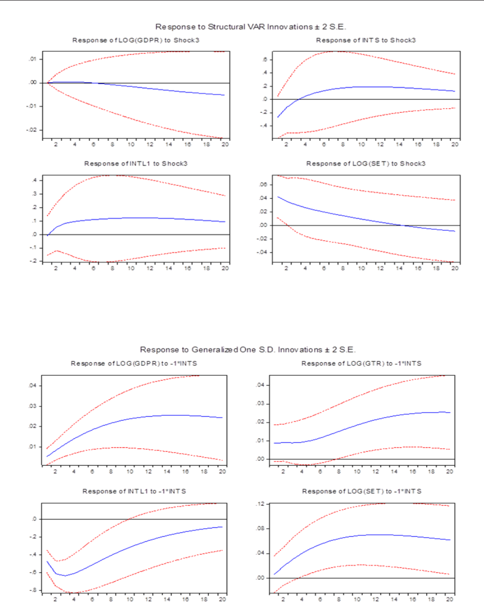
Next, we considered the effect of scal policy
shock on the real and nancial sector. As presented
in Figure 2, the stock market responded signicantly
to expansionary scal policy shocks in a positive
direction; however, the effect lasted only a few quarters.
The scal policy insignicantly affected output growth.
These results show that scal policy has only a short-
term effect on the stock market. In sum, monetary
policy and scal policy provide a signicant impact
on the stock market.
The Reduced-Form VAR With Generalized Impulse
Response Function
Similar to the previous section, we used the data
in level to estimate the reduced-form VAR model with
one lag based on minimized SIC criteria. The GIRFs
to monetary and scal policy shocks are presented in
Figures 3 and 4, respectively. The interpretation of the
GIRFs is similar to that of the previous section.
Figure 3 presents the responses of the variables to a
decrease in interest rate. As can be seen, the results are
similar to those for the SVAR model, as the real GDP
Figure 1. Impulse-response function. Y-axis, percent response to 1 standard deviation monetary policy shock (shock 4,
particularly); X-axis, quarters after shock. Blue and red lines – response and 95% condence interval, respectively.
60
S. Prukumpai, et al
Figure 2. Impulse-response function. Note: Y-axis, percent response to 1 standard deviation scal policy
shock (shock 3, particularly); X-axis, quarters after shock. Blue and red lines – response and 95% condence
interval, respectively.
Figure 3. Impulse-response function. Note: Y-axis, percent response to 1 standard deviation monetary policy
shock (short-run interest rate shock, particularly); X-axis, quarters after shock. Blue and red lines – response
and 95% condence interval, respectively.

How Does the Thai Stock Market Respond to Monetary and Fiscal Policy Shocks? 61
and stock market signicantly responded negatively
to monetary policy. In the case of scal policy, as
presented in Figure 4, scal policy shocks not only
affected the stock market but also had a signicant
effect on the output growth in the rst two quarters.
This result shows that scal policy has only a short-term
effect on real output and the stock market. \
In summary, based on the reduced-form VAR model
and the GIRFs, monetary policy and scal policy had
a signicant impact on both real GDP and the stock
market. Comparing the results based on the SVAR
model, the conclusion is similar—the real sector and
nancial sector responded positively to expansionary
monetary policy. In addition, the financial market
responded to the scal policy under both the SVAR
model and the reduced-form VAR model. This conrms
the signicant impact of scal and monetary policy on
the nancial sector.
How Do the Sector Indices Respond to Monetary
Policy and Fiscal Policy?
Several papers have examined the impact of
monetary and scal policy on stock markets, notably
Afonso and Sousa (2011), Chatziantoniou et al. (2013),
Thanh et al. (2017), and Hu et al. (2018). None of
these papers has addressed the issues examined here,
namely, the effects of monetary and scal policy on
stock markets at the sectoral level. The closest to our
study is that of Guerin and Leon (2017). However, they
investigated how changes in sectoral connectedness
will affect the response of the stock market to monetary
policy. Guerin and Leon (2017) found that highly
interconnected stock market is more likely to respond
to monetary policy. Additionally, the industry that is
more related to an aggregated market tends to react
relatively more to monetary policy shocks. Therefore,
in our study, we hypothesized that different sectors may
Figure 4. Impulse-response function. Note: Y-axis, percent response to 1 standard deviation scal policy
shock (spending shock, particularly); X-axis, quarters after shock. Blue and red lines – response and 95%
condence interval, respectively.

62
S. Prukumpai, et al
respond to monetary and scal policy differently. Due
to regularly adjusted components of sector indices by
the SET, only 18 sectors with completed data during
our study period (1996 to 2017) were included in our
analysis. The list of the sectors and their abbreviation
is shown in Table 3. All of the data were collected from
the CEIC database at a quarterly frequency.
The structural VAR model using the 18 sector
indices in place of the SET index was rst estimated.
The impulse responses of stock prices at the sectoral
level were calculated for the shocks in monetary policy
and scal policy. The results are shown in Figures 5 and
6, respectively. Figure 5 shows that all of the sectors
reacted negatively to monetary policy, similar to how
the overall market did. Unlike the monetary policy,
as presented in Figure 6, most sectors, except for the
professional service sector, positively responded to
scal policy.
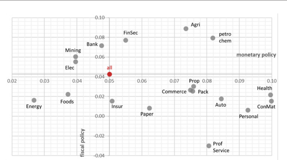
Next, we summarized the maximum response
value for each sector to policy shocks over the rst 20
quarters. The response value and response duration
for each sector are presented in Table 4. Additionally,
Figure 7 shows the sectoral response to both scal and
monetary policies.
As can be seen in Figure 7, three sectors in the rst
quadrant, namely PETROCHEM, AGRI, and FINSEC,
tended to respond to both monetary and scal policy
more than the overall market. While two sectors in
the third quadrant—ENERGY and FOODS—were less
likely to respond to either monetary or scal policy
than the market average.
Table 3
Abbreviation of Sector Indices
Sector index Abbreviation Sector index Abbreviation
Commerce COMMERCE Petrochemicals& Chemicals PETROCHEM
Banking BANK Electronic Components ELECTRONICS
Finance & Securities FINSEC Energy & Utilities ENERGY
Insurance INSUR Property Development PROP
Construction materials CONMAT Mining MINING
Agribusiness AGRI Paper & Printing Materials PAPER
Personal Products &
Pharmaceuticals
PERSONAL Packaging PACKAGING
Food and beverage FOODS Health Care Services HEALTH
Automotive AUTO Professional Services PROFSERVICE
Source: Retrieved from https://www.set.or.th/en/products/index/setindex_p2.html

How Does the Thai Stock Market Respond to Monetary and Fiscal Policy Shocks? 63
Figure 5. . Impulse-response function by sector. Note: Y-axis, percent response to 1 standard deviation monetary policy shock (shock 4, particularly); X-axis,
quarters after shock. Blue and red lines – response and 95% condence interval, respectively. Sector indices’ abbreviations are shown in Table 3.

64
S. Prukumpai, et al
Figure 6. . Impulse-response function by sector. Note: Y-axis, percent response to 1 standard deviation scal policy shock (shock 3, particularly); X-axis, quarters
after shock. Blue and red lines – response and 95% condence interval, respectively. Sector indices’ abbreviations are shown in Table 3.

How Does the Thai Stock Market Respond to Monetary and Fiscal Policy Shocks? 65
Table 4
Sectoral response value and response duration
Sector
Response to monetary policy Response to scal policy
Max value Duration Max value Duration
Overall 0.0500 8 0.0426 1
AGRI 0.0735 8 0.0888 4
FOODS 0.0372 8 0.0223 2
BANK 0.0476 8 0.0718 3
COMMERCE 0.0749 8 0.0268 4
CONMAT 0.0998 8 0.0156 1
AUTO 0.0844 8 0.0177 1
ELEC 0.0395 8 0.0553 4
ENERGY 0.0268 8 0.0162 1
FINSEC 0.0550 8 0.0771 1
INSUR 0.0508 8 0.0154 1
MINING 0.0395 8 0.0605 1
PACK 0.0756 8 0.0255 1
PAPER 0.0623 8 0.0082 1
PERSONAL 0.0926 8 0.0063 1
PROFSERVICE 0.0806 8 -0.0298 1
HEALTH 0.0995 8 0.0219 1
PETROCHEM 0.0818 8 0.0795 1
PROP 0.0759 8 0.0304 1
Note: The max value represents the maximum percent response to 1 standard deviation of policy shock while duration refers to the quarter
in which the percent response reached the maximum value.
66
S. Prukumpai, et al
When the government decided to implement
monetary policy by increasing the short-term interest
rate, the largest impact was on HEALTH, CONMAT,
and PERSONAL. One possible reason was that the
price-to-earnings (P/E) ratio of these sectors was higher
than the overall market—HEALTH’s P/E was 36.02 and
PERSONAL’s P/E was 19.39—compared to the overall
market P/E at 19.33.
1
Specically, when prices are
high, they are more sensitive to interest rate changes.
ELECTRONICS, FOODS, ENERGY, and MINING
were less affected by monetary policy. These sectors’
P/E were lower than the overall market, and the P/E
ranged from 7.69 to 20.24.
AGRI and PETROCHEM responded to fiscal
policy, changes in government spending in particular,
more than the others did. This was not surprising
because most Thai government spending programs
were related to agricultural products and infrastructure
construction and maintenance.
Conclusion
Comparing the empirical evidence on the effects
of monetary policy on the real and nancial economy,
Figure 7. Sector index response to policies shocks. Note: Y-axis, percent response to 1 standard deviation scal
policy shock (spending shock, particularly); X-axis, percent response to 1 standard deviation
monetary policy shock (short-run interest rate shock, particularly).
that of scal policy has received less attention. With
the recent economic downturn, scal policy has been
implemented more since it was expected to be effective
in terms of economic recovery. This is not the rst paper
to study the effects of monetary and scal policies;
however, most of the existing literature uses data from
developed countries. The biggest contribution of this
study is in analyzing the impact of Thai monetary and
scal policies on the stock market, both at the market
aggregate level and at the sectoral level. The ndings
can provide a reference point for research in this eld
using developing country data.
This study used quarterly data from 1996 to 2017 to
study how the Thai Stock Market responds to monetary
and scal policy. The structural VAR model with six
variables—world import volume (IMW), real GDP
(GDPR), real government spending (GTR), short-term
interest rate (INTS), long-term government bond yield
(INTL), and stock market indices (SET)—was estimated
and the following conclusions were drawn. First, based
on the causality test, monetary policy was seen to have
a bi-directional causal relationship with the real sector
but not with the stock market. No signicant causal
relationship between scal policy and either the real

How Does the Thai Stock Market Respond to Monetary and Fiscal Policy Shocks? 67
sector or the stock market was found. In addition, we
found no evidence of the crowding out effect but we
did nd a causal relationship from scal policy to
monetary policy.
Second, according to the impulse response analysis,
when comparing the results based on the SVAR model
and the reduced-form VAR model, the conclusion
was similar where the real sector and nancial sector
responded positively to expansionary monetary policy.
The impact of the scal policy was faster but lasted a
shorter length of time than that of monetary policy.
Our results reveal that the nancial market responds
to scal policy under both the SVAR model and the
reduced-form VAR model. This implies that investors
should consider both monetary and scal policy when
making investment decisions.
Exploring the response of the stock market to
policy shocks at the sectoral level, we found that
different sectors appear to react heterogeneously
to monetary and scal policy. Particularly, the high
P/E ratio sectors, such as healthcare and personal
service, were seen to be more sensitive to changes
in interest rates and vice versa. Moreover, changes
in government expenditure had the largest impact on
the agribusiness and petrochemical sectors. This is
because most monetary policy programs are related
to the promotion of agricultural product prices and
the investment in infrastructure construction and
maintenance. The heterogeneity responses of each
sector to economic policy imply that policymakers
need to customize their policies to meet the specic
needs of the sectors.
Endnote
1
The P/E ratio was retrieved from http://siamchart.
com/stock/SECTOR. October 27, 2018.
References
Afonso, A., & Sousa, R. M. (2011). What are the effects of
scal policy on asset markets? Economics Modelling,
28, 1871–1890.
Ardagna, S. (2009). Financial markets’ behavior around
episodes of large changes in the scal stance. European
Economic Review, 53, 37–55.
Bjornland, H., & Leitemo, K. (2009). Identifying the
interdependence between US monetary policy and
the stock market. Journal of Monetary Economics, 56,
275–282.
Blanchard, O., & Perotti, R. (2002). An empirical
characterization of the dynamic effects of changes in
government spending and taxes on output. Quarterly
Journal of Economics, 117, 1329-1368.
Chatziantoniou, I., Duffy, D., & Filis, G. (2013). Stock market
response to monetary and scal policy shocks: Multi-
country evidence. Economic Modelling, 30, 754–769.
Chevapatrakul, T. (2015). Monetary environments and stock
returns: International evidence based on the quantile
regression technique. International Review of Financial
Analysis, 38, 83–108.
Conover, C. M., Jensen, G. R., Johnson, R. R., & Mercer, J. M.
(1999). Monetary environments and international stock
returns. Journal of Banking and Finance, 23, 1357–1381.
Darrat, A. (1988). On scal policy and the stock market.
Journal of Money Credit and Banking, 20, 353–363.
Fama, E. F. (1970). Efcient capital markets: A review of
theory and empirical work. Journal of Finance, 25,
383–417.
Flannery, M. J., & Protopapadakis, A. A. (2002).
Macroeconomic factors do inuence aggregate stock
returns, Review of Financial Studies, 15, 751–782.
Foresti, P., & Napolitano, O. (2017). On the stock market
reactions to scal policies. International Journal of
Finance and Economics, 22, 296–303.
Goldsmith, R. (1969). Financial structure and development.
New Haven: Yale University Press.
Guerin, P., & Leon, D. L. (2017). Monetary policy, stock
market and sectoral comovement (Documentos de
Trabajo No. 1731). Madrid: Banco de Espana.
Hsing, Y. (2013). Effects of scal policy and monetary policy
on the stock market in Poland. Economies, 1, 19–25.
Hu, L., Han, J., & Zhang, Q. (2018). The impact of monetary
and scal policy shocks on stock markets: Evidence
from China. Emerging Markets Finance and Trade, 54,
1856–1871.
Jensen, G. R., & Johnson, R. R. (1995). Discount rate changes
and security return in the U.S., 1962–1991. Journal of
Banking and Finance, 19, 79–95.
Kim, S.-J., & Nguyen, T. (2009). The spillover effects of target
interest rate news from the U.S. Fed and the European
Central Bank on the Asia-Pacic stock markets. Journal
of International Financial Markets, Institutions and
Money, 19, 415–431.
Levine, R. (1997). Financial development and economic
growth: Views and agenda. Journal of Economic
Literature, 35, 688–726.
Laopodis, N. T., & Sawhney, B. L. (2002). Dynamic interactions
between Main Street and Wall Street. Quarterly Review
of Economics and Finance, 42, 803–815.
Luintel, B. K., & Khan, M. (1999). A quantitative re-
assessment of the nance-growth nexus: Evidence from
a multivariate VAR. Journal of Development Economics,
60, 381–405.

68
S. Prukumpai, et al
MacKinnon, J. G. (1990). Critical values for cointegration
tests (Queen’s Economics Department Working Paper
No. 1227) Ontario: Queen’s University.
McKinnon, R. I. (1973). Money and capital in economic
development. Washington, D.C.: Brookings Institution.
Melitz, J. (1997). Some cross-country evidence about
debt, decits and the behavior of monetary and scal
authorities (CEPR Discussion Paper No. 1653). London:
CEPR.
Mishkin, F. S. (1996). The channels of monetary transmission:
Lessons for monetary policy (NBER Working Paper No.
5464). Massachusetts: National Bureau of Economic
Research.
Muscatelli, V. A., Tirelli, P., & Trecroci, C. (2004). Fiscal and
monetary policy interactions: Empirical evidence and
optimal policy using a structural New-Keynesian model.
Journal of Macroeconomics, 26, 257–280.
Pesaran, M. H., & Shin, Y. (1998). Generalized impulse
response analysis in linear multivariate models.
Economics Letters, 58, 17–29.
Ramey, V. A., & Shapiro, M. D. (1998). Costly capital
reallocation and the effects of government spending.
Carnegie-Rochester Conference Series on Public Policy,
48, 145–194.
Rigobon, R., & Sack, B. (2003). Measuring the reaction of
monetary policy to the stock market. Quarterly Journal
of Economics, 118, 639–669.
Sims, C. A. (1980). Macroeconomics and reality. Econometrica:
Journal of the Econometric Society, 48, 1–48.
Thanh, T. T., Thuy, L. P., Anh, T. N., Thi, T. D., & Truong, T.
H. (2017). Empirical test on impact of monetary policy
and scal policy on Vietnam stock market. International
Journal of Financial Research, 8, 135–144.
Thorbecke, W. (1997). On stock market returns and monetary
policy. Journal of Finance, 52, 635–654.
Tobin, J. (1969). A general equilibrium approach to monetary
theory. Journal of Money Credit and Banking, 1,
15–29.
Vithessonthi, C., & Techarongrojwong, Y. (2013). Do
monetary policy announcements affect stock prices
in emerging market countries? The case of Thailand.
Journal of Multinational Financial Management, 23,
446–469.
Wongswan, J. (2009). The response of global equity indexes
to U.S. monetary policy announcements. Journal of
International Money and Finance, 28, 344–365.
