The Long-term Decline of the U.S. Job Ladder

Aniket Baksy

Daniele Caratelli

†

Niklas Engbom

‡

April 26, 2024

Abstract

We develop a methodology to consistently estimate employer-to-employer (EE) mobility toward

higher paying jobs based on publicly available microdata from the Current Population Survey,

and use it to document three trends over the past half century. First, such EE mobility fell

by half between 1979 and 2023. Second, its decline reduced annual wage growth by over one

percentage point. Third, the decline was particularly pronounced for women, those without a

college degree, and young workers. The decline does not appear to primarily stem from work-

ers being better matched with their current jobs or the labor market being worse at matching

workers and ﬁrms. Instead, based on long-run variation across U.S. states, we present evidence

consistent with the view that greater labor market concentration reduced workers’ opportuni-

ties to transition toward higher paying employers.

Digital Futures at Work Research Center, University of Sussex: [email protected]

†

Ofﬁce of Financial Research, U.S. Department of the Treasury: [email protected]

‡

CEPR, NBER, UCLS and New York University Stern School of Business: [email protected]

The views and opinions expressed are those of the authors and do not necessarily represent ofﬁcial positions of the

Ofﬁce of Financial Research or the U.S. Department of the Treasury. We thank Sadhika Bagga, Adam Blandin, Katarina

Borovickova, Kyle Herkenhoff, Loukas Karabarbounis, Ricardo Lagos, Claudia Macaluso and Venky Venkateswaran

for useful comments.

1 Introduction

Shopping for jobs is an integral part of workers’ careers. Young workers enter the labor mar-

ket poorly matched, and gradually relocate across ﬁrms to ﬁnd better matches. Topel and Ward

(1992) ﬁnd that this process of employer-to-employer (EE) reallocation toward higher paying jobs

accounts for a third of workers’ wage growth during the ﬁrst 10 years of their careers. More re-

cently, macroeconomists have stressed that such reallocation also plays a critical role for aggregate

economic performance, by reallocating workers from less to more productive ﬁrms (Lentz and

Mortensen, 2012; Moscarini and Postel-Vinay, 2017). Yet, despite its importance for both micro

and macroeconomic outcomes, little is known about long-run trends in such reallocation.

The reason is twofold. First, the data required to measure the frequency at which workers

move from one employer to another without an intervening spell of nonemployment are only

available since the mid-1990s. Furthermore, the series available from the main labor force sur-

vey in the U.S., the Current Population Survey (CPS), suffers from bias arising from changes in

survey methodology and non-response over time (Fujita, Moscarini and Postel-Vinay, Forthcom-

ing).

Second, many EE transitions in the raw data are toward lower paying jobs (Tjaden and

Wellschmied, 2014; Sorkin, 2018). Of particular interest for macroeconomic performance, how-

ever, is EE mobility toward higher paying, more productive jobs—what we henceforth refer to as

allocative EE mobility (Bilal et al., 2022; Elsby and Gottfries, 2022).

This paper proposes a methodology that overcomes these dual challenges, and uses it to docu-

ment three trends in allocative EE mobility over the past half century in the U.S. based on publicly

available micro data from the CPS. First, allocative EE mobility fell in half between 1979 and 2023.

Second, ceteris paribus the decline reduced annual wage growth by over one percentage point.

Third, the fall was particularly pronounced for women, those without a college degree, and young

workers. In terms of potential explanations, we ﬁnd little support for the notion that allocative EE

mobility is lower today because workers are better matched with their current employers (Mer-

can, 2017; Pries and Rogerson, 2022) or the labor market is worse at matching workers and ﬁrms.

Instead, based on long-run variation across U.S. states, we provide evidence consistent with the

view that greater labor market concentration reduced workers’ opportunities to transition toward

higher paying employers (Bagga, 2023; Berger et al., 2023; Jarosch, Nimczik and Sorkin, 2024).

Our point of departure is a prototypical job ladder model in the spirit of Burdett and Mortensen

(1998). In each period, non-employed and employed workers receive job offers with some exoge-

nous and potentially different probability. A job offer is a draw of a wage from an exogenous

wage offer distribution, which may also vary by employment status (Faberman et al., 2022). If the

worker accepts the job, she supplies a unit of labor at the speciﬁed wage until either she ﬁnds a

An alternative, arguably superior, series is available from the Survey of Income and Program Participation (SIPP), but

high-quality data are only available for 1996–2013.

We borrow this terminology from the literature, but caution that it should be interpreted from the perspective of a

social planner who does not face any frictions and who aims to maximize aggregate output.

new job offering a higher wage or her job exogenously terminates and she becomes non-employed.

The model predicts that the number of workers earning at most a wage w in period t + 1

depends on the number of workers paid at most w in period t, the number of these workers who

separated to non-employment between periods t and t + 1, the number of non-employed workers

in period t who found a job paying at most w in period t + 1, and the fraction who made an EE

transition to a job paying more than w between t and t + 1. Knowledge of all the other objects in

this relationship allows us to recover the EE transition probability.

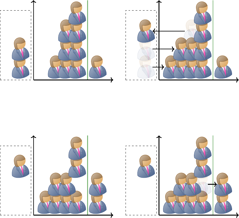
The logic is best explained via the example in Figure 1. Consider a labor market in which eight

workers earn a wage below w in each period t. Suppose that between periods t and t + 1, one of

these workers separates to non-employment, while two workers are hired from non-employment

into jobs paying less than w. Suppose that in period t + 1, we again observe eight workers earning

less than w. We are interested in what fraction x(w) of workers employed at a wage less than w

that made an EE transition to jobs paying more than w. It solves

|{z}

earning ≤ w at t

− 1

|{z}

employment outﬂows

+ 2

|{z}

employment inﬂows

− 8x(w)

|{z}

EE moves from ≤ w to > w

= 8

|{z}

earning ≤ w at t + 1

Hence, x( w) = 12.5 percent of workers earning less than w made an EE transition to a job paying

more than w. Knowledge of this share as well as the share of all workers who are paid w for each

wage w allows us to compute the overall EE transition probability to higher paying jobs.

To measure the inputs required to estimate allocative EE mobility, we use data from the ba-

sic monthly survey and the Outgoing Rotation Group (ORG) of the CPS. Speciﬁcally, we record an

individual’s employment status in each month during a four month period, her hourly wage in

the last of these four months, and demographic characteristics. Since our model assumes that all

wage growth is due to EE mobility, we residualize wages on a rich set of demographic controls

that account for wage growth with experience as well as for the impact of aggregate trends. Sub-

sequently, we measure the share of workers earning less than (residual) wage w in months t and

t + 1, the share of hires from non-employment who earn a wage below w in month t + 1, and the

share of employed workers in month t who are non-employed in period t + 1. Through the lens

of our theory, these objects are sufﬁcient to recover allocative EE mobility in month t.

We validate our methodology by contrasting our measure of allocative EE mobility to raw EE

mobility in the CPS since 1994, in the SIPP between 1996 and 2013, and for the cohort of individu-

als who were 14–22 years old in 1979 in the National Longitudinal Survey of Youth 1979 (NLSY ’79).

We ﬁnd that raw EE mobility is higher in the CPS than in the SIPP, which in turn is higher than al-

locative EE mobility. Consistent with evidence that changes in non-response rates in the CPS bias

raw EE mobility toward an excessively large decline (Fujita, Moscarini and Postel-Vinay, Forth-

coming), allocative EE mobility shows a smaller decline since the early 2000s. Raw EE mobility

toward a higher paying job in the SIPP is, however, close to our estimate of allocative EE mobility.

Date t Stocks

Wage

Nonemployed

Date t Flows

Wage

Nonemployed

Date t + 1 Stocks

Wage

Nonemployed

Inferred EE Flows

Wage

Nonemployed

Figure 1: Identifying EE mobility using microdata. Suppose that eight individuals earn (weakly)

less than w in period t. Between periods t and t + 1, one of these individuals separates into

nonemployment, while two previously nonemployed individuals enter employment at a wage

(weakly) less than w. In period t + 1, we again observe eight individuals earning (weakly) less

than w. We conclude that one individual who earned less than w in period t made an EE transition

to a job paying more than w in period t + 1, corresponding to 12.5% of workers.

Furthermore, allocative EE mobility among the cohort that turned 14–22 in 1979 matches well raw

EE mobility toward higher paying jobs over the 1981–2018 period in the NLSY ’79.

Having validated our methodology, we use it to establish three trends in allocative EE mobil-

ity in the U.S. over the past half century. First, allocative EE mobility declined sharply since the

mid-1980s, falling from 1.5 percent per month to less than one percent today (with only a short-

lived reversal during the Pandemic). Second, ceteris paribus the fall in allocative EE mobility is

associated with a sizeable decline in wage growth, as workers climbed the job ladder less. Our

estimates imply that allocative EE mobility contributed over three percentage points to annual

real wage growth in the 1980s. As such mobility declined, so did the wage gains associated with

it. In fact, despite an increase in the average wage gain conditional on an allocative EE transition,

the declining frequency of such transitions contributed to over one percentage point weaker an-

nual wage growth today. Third, although the decline in allocative EE mobility and its associated

wage growth were pervasive across demographic groups, they were particularly pronounced for

women, workers without a college degree, and young workers.

While our methodology allows us to provide new evidence on long-run trends in allocative

EE mobility, it does so by imposing three strong assumptions. First, we assume that job ladder

dynamics is the sole source of residual wage growth, consistent with recent work highlighting the

central role of EE mobility for wage dynamics (Karahan et al., 2017; Moscarini and Postel-Vinay,

2017; Ozkan, Song and Karahan, 2023; Tanaka, Warren and Wiczer, 2023). Second, we impose that

the recently non-employed are not systematically different in unobservable dimensions than their

identical looking peers. Third, we abstract from EE transitions toward lower paying jobs.

To assess the sensitivity of our results to these strong assumptions, we turn to three extensions.

First, we allow also for residual wage growth with tenure, ﬁnding that such wage growth is uni-

formly small over our sample period so that allowing for it makes little difference to our results.

Second, we use the fact that we can observe wages twice in order to residualize a worker’s current

wage also off her previous wage as a control for unobservable characteristics. Although doing

so (modestly) lowers the level of allocative EE mobility—consistent with recently non-employed

workers being worse in unobservable ways—it has little effect on the decline in allocative EE mo-

bility over this period. The reason is that such negative selection on unobservables did not change

over time. Third, we incorporate undirected EE mobility following Jolivet, Postel-Vinay and Robin

(2006) in order to match the overall level of EE mobility in the data. While such mobility is com-

mon, allowing for it substantively changes neither the level nor the trend in allocative EE mobility.

We end with an assessment of three prominent potential explanations for the decline in alloca-

tive EE mobility. One possibility is that workers today are better matched in the labor market, so

that they are less likely to accept an outside job offer (Mercan, 2017; Pries and Rogerson, 2022).

Under the standard assumption that the non-employed and employed sample wage offers from

the same distribution, we show that we can separately identify the job ﬁnding probability of the

employed and the probability that they accept an extended offer. We estimate that the acceptance

probability modestly rose over time.

Hence, the decline in allocative EE mobility is entirely ac-

counted for by a lower probability that an employed worker receives an outside job offer. Molloy

et al. (2016) draw a similar conclusion that workers are not better matched today based on the lack

of a long-run trend in starting wages.

Second, the decline in the job ﬁnding probability of the employed could, for instance, be the

We stress that this refers to the acceptance probability of the employed, not the acceptance probability of the non-

employed, which Birinci, See and Wee (2023) ﬁnd has declined.

result of changes in the efﬁciency with which the labor market matches workers and ﬁrms. Alter-

natively, ﬁrms might advertise fewer job openings today. Benchmark equilibrium theories of the

labor market predict that such forces proportionately reduce the job ﬁnding probability of the em-

ployed and non-employed. In contrast, we ﬁnd that the job ﬁnding probability of the employed

declined by much more than that of the non-employed, suggesting that the decline in EE mobility

was not primarily the result of changes in matching efﬁciency or ﬁrms’ recruitment efforts.

Our results instead point to factors that particularly impacted the job ﬁnding prospects of the

employed. Two hypotheses consistent with this pattern are reduced search intensity of the em-

ployed, perhaps stemming from the increased use of non-compete agreements that discourages

on-the-job search (Gottfries and Jarosch, 2023), or greater labor market concentration which lim-

its workers’ outside options (Bagga, 2023; Berger et al., 2023; Jarosch, Nimczik and Sorkin, 2024).

In line with the latter view, we document that the job ﬁnding probability of the employed de-

clined disproportionately in U.S. states that saw larger increases in labor market concentration.

Speciﬁcally, we replicate our analysis for each state plus Washington D.C., and merge the result-

ing data set with measures of the number of ﬁrms per worker and the prevalence of large ﬁrms

from the U.S. Census Business Dynamic Statistics (BDS). We project the job ﬁnding probability of

the employed at the state-5-year period level on various measures of labor market concentration,

controlling for state and time ﬁxed effects. Our results reveal that labor market concentration is

strongly negatively correlated with the job ﬁnding probability of the employed, but only weakly

so with that of the non-employed. Indeed, the point estimate would imply that the increase in

labor market concentration observed at the national level between 1979 and today accounts for

more than 40 percent of the fall in allocative EE mobility over this period.

Literature. This paper contributes to a literature studying the decline in economic “dynamism”

in the U.S. over the past ﬁfty years. Following Steve Davis’ and John Haltiwanger’s pioneering

work, several papers document large declines in the rates of job creation and destruction in the

U.S. since the early 1980s (Davis and Haltiwanger, 2014; Decker et al., 2016). Due to data limita-

tions, however, less is known about long-run trends in worker ﬂows, in particular EE mobility.

Fallick and Fleischman (2004) is the ﬁrst paper to use the introduction of “dependent inter-

viewing” techniques to the CPS to estimate EE mobility back to 1994. Fujita, Moscarini and Postel-

Vinay (Forthcoming) note that selective non-response biases the CPS toward showing an exces-

sively large decline in EE mobility, and propose a corrected version that displays a more muted

decline. Hyatt and Spletzer (2013), Hyatt (2015) and Haltiwanger et al. (2018) study trends in EE

mobility using matched employer-employee data from the Longitudinal Employer-Household

Dynamics (LEHD) program starting in 1998. Several papers proxy the EE transition probability

using the number of employers a respondent had in the previous calendar year (Blanchard and

Diamond, 1990; Shimer, 2005; Diamond and S¸ahin, 2016; Molloy et al., 2016), but this is an imper-

fect proxy because it risks misclassifying, for instance, employment-unemployment-employment

transitions as EE transitions. Hyatt and Spletzer (2016, 2017) and Molloy, Smith and Wozniak

(2024) infer changes in worker mobility based on the tenure distribution. In addition to allowing

us to consistently estimate EE mobility starting in 1979, an advantage of our methodology is that

it isolates the component of EE mobility that is toward higher paying jobs. Jolivet, Postel-Vinay

and Robin (2006) apply a job ladder model similar to ours to cross-country data in order to infer

the rate at which workers move up the job ladder. Our motivation is shared by Shimer (2012),

who uses a parsimonious model of labor market ﬂows to unemployment duration data to infer

the separation probability to and job ﬁnding probability from unemployment starting in 1948.

Our paper is also related to a rapidly growing literature that studies the impact of labor mar-

ket power on wages and employment (Macaluso, Hershbein and Yeh, 2019; Azar et al., 2020;

Prager and Schmitt, 2021; Azar, Marinescu and Steinbaum, 2022; Berger, Herkenhoff and Mon-

gey, 2022; Benmelech, Bergman and Kim, 2022; Handwerker and Dey, 2022; Rinz, 2022; Caldwell

and Danieli, 2024). Most closely related, Bagga (2023) ﬁnds a positive correlation between EE mo-

bility and the ratio of ﬁrms to workers across U.S. local labor markets. Due to data limitations,

however, she is restricted to analyze the cross-sectional relationship, as opposed to the within-

state patterns that we study. While both papers lack a credible identiﬁcation strategy to obtain

a causal estimate, within-region variation arguably reduces concerns about third factors driving

the correlation. Berger et al. (2023) correlate measures of market concentration with worker ﬂows

both across and within local labor markets in Norway between 2006 and 2018. Consistent with our

result, they ﬁnd a negative relationship between the two. Our result complements their ﬁnding by

offering a longer time series and by providing evidence from the U.S., whose institutional setting

may differ in important dimensions from Norway’s.

We start by outlining our partial equilibrium job ladder model in section 2. Section 3 discusses

the data and our estimation procedure. In section 4, we present three facts on long-term trends

in EE mobility and its associated wage growth. Section 5 incorporates three extensions. Section 6

evaluates three prominent explanations for the decline in EE mobility. Finally, section 7 concludes.

2 A Prototypical Job Ladder Model

This section outlines a parsimonious partial equilibrium model of worker dynamics in the spirit

of Burdett and Mortensen (1998) set in discrete time. The job ﬁnding probabilities, the separation

probability, and the wage offer distribution are all taken as exogenous. While stylized, an exten-

sive literature ﬁnds that this framework is quite successful at matching empirical labor market

dynamics (Jolivet, Postel-Vinay and Robin, 2006).

2.1 Environment

Time t ≥ 0 is discrete and inﬁnite. A unit mass of ex-ante identical, inﬁnitely-lived workers move

across jobs as well as in and out of employment. Let e

denote the employment rate at time t.

Non-employed workers receive job offers with exogenous probability λ

∈ [0, 1]. A job offer

is a draw of a (log) wage w from an exogenous wage offer distribution of the non-employed. Let

t+1

( w) denote its probability density function (pdf) and F

t+1

( w) its cumulative distribution func-

tion (cdf), with support w ∈ (−∞, ∞). We assume that non-employed workers accept any job

offer they receive.

The wage remains ﬁxed for the duration of the match.

With exogenous probability λ

∈ [0, 1], an employed worker receives an outside offer from

a wage offer distribution of the employed, whose pdf (cdf) we denote f

t+1

( w) (F

t+1

( w)). Since

workers choose whether to accept an offer, they only switch to jobs that offer higher wages. We

refer to the resulting mobility toward higher paying jobs as allocative EE mobility.

Finally, employed workers separate to non-employment with exogenous probability δ

∈ [0, 1].

We require that these probabilities satisfy δ

+ λ

≤ 1.

2.2 Labor market ﬂows

The number of workers earning wage w at time t, g

( w)e

, evolves according to

t+1

(

)

t+1

= g

( w)e

− δ

( w)e

| {z }

separations to nonemp.

−λ

(

1 − F

t+1

( w)

)

( w)e

| {z }

EE separations

(1)

+ λ

t+1

( w)(1 − e

)

| {z }

hires from nonemp.

+ λ

t+1

( w)G

( w)e

| {z }

EE hires

Integrating (1) from −∞ to w, applying integration by parts, gives

t+1

(

)

t+1



1 −δ

−λ

(1 − F

t+1

( w))



( w)e

+ λ

t+1

( w)(1 − e

)

which we can rearrange as



1 − F

t+1

( w)



| {z }

sep

(w)≡poaching separation probability

= 1 −

t+1

( w)

t+1

+ λ

t+1

( w)

1 −e

− δ

(2)

We discuss below how to measure G

( w), G

t+1

( w), F

t+1

( w), e

, e

t+1

, λ

and δ

in the CPS. Provided

these objects, we can estimate the poaching separation probability at each wage w based on (2). The

This assumption can be motivated by the fact that no ﬁrm would ﬁnd it optimal to advertise a job paying less than

the reservation wage common to all non-employed workers.

Integrating by parts the EE separations term in (1) gives

−∞

(1 − F

t+1

(

w))g

(

w) d

w = (1 − F

t+1

(w))G

(w) +

−∞

t+1

(

w)G

(

w)d

w. The last term cancels the integrated EE hires term.

EE transition probability is then the average poaching separation rate

= λ

∞

−∞



1 − F

t+1

( w)



( w) =

∞

−∞

sep

( w)dG

( w) (3)

The EE transition probability can be written as the product of the probability that an employed

worker receives a job offer and the average probability of the worker accepting the offer

= λ

|{z}

job ﬁnding probability

∞

−∞



1 − F

t+1

(

)



(

)

| {z }

acceptance probability

(4)

Hence, EE mobility can fall either because workers are less likely to receive job offers or because

they are less likely to accept them. While we do not need to measure the wage offer distribution

of the employed to estimate overall EE mobility (3), the decomposition (4) requires it. Since it is

fundamentally unobserved,

to implement (4) we follow much of the literature in assuming that

the employed sample jobs from the same distribution as the non-employed, f

( w) = f

( w).

2.3 Wage growth due to EE mobility

Wage growth due to EE mobility is the fraction of workers who receive a job offer times the average

wage gain conditional on accepting it

∆w

= λ

∞

−∞

∞



w − w



t+1

(

w)dG

( w) = λ

∞

−∞



w −



(

w) dF

t+1

( w)

Integrating by parts and using the fact that lim

w→∞

t+1

( w) = 1, we have

∆w

= λ

∞

−∞





h

w −



(

w=−∞

−∞

(

w)d





t+1

( w)

= λ

∞

−∞

(

w)d

wdF

t+1

( w)

= λ









−∞

(

w)d

t+1

( w)





∞

w=−∞

−

∞

−∞

( w)F

t+1

( w)dw





= λ

∞

−∞



1 − F

t+1

( w)



( w)dw

Although the wage distribution of new hires from employment can be inferred in the CPS since 1994, it is not the

same as the wage offer distribution of the employed, since employed workers reject some wage offers.

∞

−∞

sep

( w)G

( w)dw (5)

2.4 Identiﬁcation

To highlight what aspects of the data inform the level of EE mobility, we note that in steady-state,

outﬂows from and inﬂows into employment coincide, λ

(1 −e

) = δ

. Hence, if the labor market

at date t is in steady-state, the law of motion for the wage distribution (2) simpliﬁes to



1 − F

t+1

( w)



= λ

t+1

( w)

1 −e

− δ

= δ

t+1

( w) −G

( w)

(6)

Integrating (6) over all wages from −∞ to ∞ delivers

= δ

|{z}

separation probability channel

∞

−∞

t+1

( w) −G

( w)

| {z }

offer channel

(7)

Ceteris paribus, we infer a higher EE transition probability if either the separation probability

to non-employment, δ

, or the average deviation between the wage and wage offer distribution is

larger. Figure 2 illustrates the intuition by plotting the wage offer and wage distributions based

on the data constructed in the next section pooled across all years. The wage distribution ﬁrst-

order stochastically dominates the wage offer distribution, consistent with EE mobility gradually

relocating workers toward higher paying jobs. All else equal, higher EE mobility increases the

gap between the two distributions. That being said, this pattern could also be the result of other

forces such as on-the-job wage growth or the recently non-employed being negatively selected on

unobservables. We argue below that such factors are not the main driver of these patterns.

3 Estimation

We now discuss how we bring the model to the data in order to estimate allocative EE mobility.

3.1 Data

We use publicly available data from the CPS from 1979 to 2023 conducted by the Bureau of La-

bor Statistics (BLS) and made available by the Integrated Public Use Microdata Series (IPUMS) and

the National Bureau of Economic Research (NBER).

The CPS is the main U.S. labor force survey,

The ORG started in 1979, but it should be possible to extend our analysis back to 1976 using the May Supplements.

(a) Probability density function.

−1.5 −1.0 −0.5 0.0 0.5 1.0 1.5

Log residual wage

0.0

0.2

0.4

0.6

0.8

1.0

1.2

Density

(b) Cumulative distribution function.

−1.5 −1.0 −0.5 0.0 0.5 1.0 1.5

Log residual wage

0.0

0.2

0.4

0.6

0.8

1.0

1.2

Cumulative density

Wage oﬀer dist.

Wage dist.

Figure 2: Wage and wage offer distributions in the pooled CPS 1979–2023.

serving as the benchmark data set for labor market analyses. At the time of writing, IPUMS has

incorporated ORG data through March 2023.

Every month, the CPS surveys roughly 60,000 households using a rotating panel design. Specif-

ically, a household responds to the basic monthly survey in each month for four consecutive

months, rotates out of the survey for eight months, and ﬁnally returns to answer the basic monthly

survey in each month for another four consecutive months. We refer to the ﬁrst four months as

survey months 1–4 and the latter four months as survey months 5–8. While the CPS is designed

to be representative of the U.S. population, non-random attrition necessitates the use of survey

weights, which we use throughout.

For a reference week in each month, the CPS records the employment status of each house-

hold member aged 15 and older, as well as usual weekly hours for those who are employed and

job search activities during the four weeks leading up to the reference week for those who are

not employed.

Usual weekly hours are top-coded at 99 hours. In addition, basic demographic

characteristics of the household member are collected.

In the ﬁnal month before a household either temporarily or permanently leaves the sample—

i.e. in survey months 4 and 8—respondents are asked about usual weekly wage and salary earn-

ings. Earnings are before taxes and other deductions and include overtime pay, commissions and

tips. For multiple jobholders, the data reﬂect earnings at their main job. Earnings are top-coded

at thresholds that vary throughout the sample. We refer to the ﬁrst (second) wage observation

month as the ﬁrst (second) ORG month.

Prior to 1994, usual weekly hours are only recorded in the ORG.

Starting in 1994, households with varying hours do not report usual weekly hours on the main job. We replace

these with actual hours worked on the main job.

3.2 Sample selection and variable construction

We restrict attention to individuals aged 16 and older who have non-missing age, race, gen-

der and education, and who live in one of the 50 U.S. states or Washington D.C. We drop self-

employed individuals, since weekly earnings are only recorded for wage and salary employees.

Changes to individual identiﬁers prevent linking individuals in the following breaks: June-July

1985, September-October 1985, and May-October 1995.

We aggregate race to white, black and other, and education to less than high school, a high-

school diploma, some college, a bachelor’s degree, and more than a bachelor’s degree. We top-

code age at 75 years. Occupations are recoded to the 2010 classiﬁcation. We multiply top-coded

weekly earnings by 1.5 following standard praxis.

We link individuals across survey months as well as between the basic monthly/ORG using

the consistent ID created by IPUMS (CPSIDV).

It links individuals based on household identiﬁers,

person identiﬁers, age, sex, and race.

We classify individuals in each month as wage employed, self-employed, unemployed and

not in the labor force following standard practice. Since at least Clark and Summers (1979), it has

been recognized that the distinction between unemployment and not in the labor force is fuzzy.

Consequently, we classify all unemployed and not in the labor force as non-employed.

We estimate the separation probability to non-employment δ

as the share of wage employed

individuals in month t who are non-employed in month t + 1. We estimate the job ﬁnding proba-

bility of the non-employed λ

as the share of non-employed individuals in month t who are wage

employed in month t + 1. Due to inability to link individuals in the breaks mentioned above, we

cannot compute these ﬂow rates in June 1985, September 1985, and May-September 1995.

We construct the hourly real wage as usual weekly earnings divided by usual weekly hours

worked, converted to 2022 USD using the CPI. Since our theory is about residual wage dispersion,

we residualize log hourly real wages off a rich set of observable characteristics (age-race-gender-

education-year dummies and state-date ﬁxed effects)

i,t

= ξ

a,r,g,e,y

+ ξ

s,t

+ ε

i,t

(8)

We also present results adding 3-digit occupation-year ﬁxed effects to (8). To estimate the unob-

servables model, we additionally include a worker’s wage 12 months earlier in (8).

Subsequently, to limit the impact of a few outliers, we winsorize residual wages at each date at

the bottom and top 0.5 percentiles. Finally, we compute N cutoffs b

such that a share i/N of ob-

servations in the pooled 1979–2023 sample earn a residual wage below b

(weighted by the survey

See https://assets.ipums.org/_files/ipums/working_papers/ipums_wp_2023-01.pdf.

We have conﬁrmed that we get a similarly large decline in EE mobility over time if we alternatively restrict attention

to only those who are formally unemployed.

weights). We construct these thresholds based on the baseline model, and use the same thresholds

consistently in all models to avoid any differences being driven by changes in the binning. We

assign b

= w, dw

= b

−b

i −1

and w

= (b

+ b

i −1

) /2. In practice, we set N = 50.

We estimate the wage offer distribution of the non-employed at time t, f

t,i

, as the (weighted)

share of hires from non-employment who earns a residual wage greater than b

i −1

but less than b

t,i

∑

i−1

≤

t,j

∗

hire

t,j

∗weight

t,j

∑

hire

t,j

∗weight

t,j

(9)

where we deﬁne a hire from non-employment at date t, hire

t,j

, as any employed individual j at

time t who was non-employed in month t −1. We estimate the wage distribution at time t, g

t,i

, as

the (weighted) share of employment who earns a residual wage greater than b

i −1

but less than b

t,i

∑

i−1

≤

t,j

∗weight

t,j

∑

weight

t,j

(10)

We subsequently construct the cdfs of the wage offer and wage distributions in the obvious way.

3.3 Estimating EE mobility and its associated wage growth

To improve the precision of our estimates of EE mobility at date t, we pool months t − T to t +

T, where in our benchmark we set T = 12. That is, we obtain a 23-month centered moving

average. Speciﬁcally, we ﬁrst assign for each outcome y

τ,i

= {G

τ,i

, G

τ+1,i

, F

τ+1,i

, g

τ,i

} and x

, e

τ+1

, λ

, δ

} in period t the average outcome between t − T and t + T

t,i

2T + 1

t+T

∑

τ=t−T

τ,i

2T + 1

t+T

∑

τ=t−T

We set the poaching separation rate in period t as

sep

t,i

= 1 −δ

−

t+1,i

t,i

t+1

+ λ

t+1,i

t,i

1 −e

(11)

Based on (3), we estimate the EE transition probability in period t as

∑

i =1

sep

t,i

(12)

While the level of EE mobility changes modestly if we change the number of grid points—we have experimented

with N = 10, N = 20, N = 100 or N = 500—the time trend is virtually identical. These results are available on request

(or can easily be reproduced by changing one global setting in the code we plan to make available for public use).

Based on (5), we estimate average wage growth due to EE mobility as

∆w

∑

i =1

sep

t,i

(13)

To implement the decomposition (4) of the EE transition probability into the job ﬁnding probability

versus the acceptance probability (which requires the assumption that f

= f

), we estimate the

job ﬁnding probability of the employed and the acceptance probability as

t,i

1 −δ

−

t+1,i

t,i

t+1

+ λ

t+1,i

t,i

1 −e

.

1 − F

t+1,i



∑

i =1

t,i

acceptance

3.4 Validation

Before we use our methodology to provide new evidence on long-run trends in allocative EE

mobility, we pause to consider three validation exercises of our methodology.

First, we contrast allocative EE mobility with measures of raw EE mobility from the CPS, SIPP

and NLSY ’79. Speciﬁcally, we construct the fraction of employed workers in month t who are

employed with a different employer in month t + 1. Additionally in the SIPP and NLSY ’79, we

compute the share of workers who make an EE transition with an associated wage gain.

Figure 3 shows a more pronounced decline in raw EE mobility in the CPS during the 2000s.

Fujita, Moscarini and Postel-Vinay (Forthcoming) argue that this is due to changes in non-response

rates that bias the raw CPS series toward showing an excessively large decline since the early

2000s. As is well-known, EE mobility is lower in the SIPP than the CPS. Allocative EE mobility is

substantially lower than raw EE mobility in both the CPS and SIPP, consistent with large EE ﬂows

toward lower paying jobs (Tjaden and Wellschmied, 2014; Sorkin, 2018). Once we condition on

those who experienced a wage gain during their transition, raw EE mobility toward higher paying

jobs is reassuringly similar in both level and changes to allocative EE mobility.

Figure 4 shows a signiﬁcant decline in EE mobility toward higher paying jobs in the NLSY ’79

over time. Because these data follow only one cohort, these changes result from both aggregate

Consistent SIPP data are available from 1996 to 2013, while data from the NLSY ’79 is available for a cohort that

turned 14–22 in 1979. The NLSY records employment status, employer ID and hourly wages on a weekly basis. We

replicate our CPS/SIPP sample by restricting attention to a main employer in one selected “survey week” of each

month. We focus in the NLSY ’79 on years 1981 (when the youngest individuals turned 16) to 2018 (when the oldest

individuals turned 60). We impose exactly the same sample selection criteria as in the CPS and residualize wages off

the same demographics (the one difference is that we cannot include state-date ﬁxed effects in the NLSY ’79, since state

identiﬁers are not made publicly available).

1992 1996 2000 2004 2008 2012 2016 2020 2024

0.0

0.5

1.0

1.5

2.0

2.5

3.0

3.5

Monthly probability (%)

Baseline CPS FMP SIPP SIPP (up)

Figure 3: Comparison between the EE transition probability implied by the baseline model (black),

the raw overall EE transition probability in the CPS (dotted light blue), the Fujita, Moscarini and

Postel-Vinay (Forthcoming) series (solid light blue), the SIPP (dotted dark blue), and the EE tran-

sition probability towards higher-paying jobs in SIPP (solid dark blue) over time. All series are

smoothed with a 23-month centered moving average.

time effects and aging of the cohort. To compare apples-to-apples, we re-estimate allocative EE

mobility for the restricted sample of individuals aged 14–22 in 1979. The decline in allocative EE

mobility starts a few years later according to the NLSY ’79 and is subsequently somewhat larger.

Yet the two series are reassuringly similar, both in levels and changes over time.

1980 1984 1988 1992 1996 2000 2004 2008 2012 2016 2020

0.0

0.5

1.0

1.5

2.0

2.5

Monthly probability (%)

Baseline

NLSY ’79

Figure 4: Monthly allocative EE transition probability according to our methodology and the raw

EE transition probability toward higher paying jobs in the NLSY ’79. Both series are for the cohort

of individuals that were aged 14–22 in 1979, and are smoothed using a 23-month moving average.

Second, we probe the assumption that the recently non-employed are not different in unob-

servable dimensions than their identical looking peers. To that end, we note that an implication

of this assumption is that wages of hires from non-employment should converge over time to the

average wage among all workers. Figure 5 plots the progression of average wages for workers

hired in month 0 from non-employment as well as the average wage of all workers. All series are

residualized off the demographic characteristics in the baseline model, and normalized relative

to initial residual wages in month 0 for hires from non-employment. Note that we do not con-

dition on continuous employment—i.e. some workers experience subsequent non-employment

spells. Since we are only able to follow workers for a short period in the CPS, we exploit also

the longer panel of the SIPP. Wages grow somewhat more with time since non-employment in the

SIPP than the CPS, consistent with a larger gap between the offer distribution and wage distribu-

tion in the former. Both data sources, however, paint a picture of gradual convergence, although it

remains incomplete (but continuing) 60 months later. This evidence is consistent with the recently

non-employed not being different than their identical looking peers in unobservable dimensions.

Nevertheless, we later consider an extension that controls for such unobserved heterogeneity.

0 10 20 30 40 50 60

0.00

0.05

0.10

0.15

0.20

Cumulative wage growth (logs)

Hires at t = 0 (SIPP)

All (SIPP)

0.00

0.04

0.08

0.12

0.16

Cumulative wage growth (logs)

Hires at t = 0 (CPS)

All (CPS)

Figure 5: Convergence in average residual wages of workers after they leave non-employment

(t = 0) toward economy-wide average residual wage. Both series are expressed in log deviations

to average wages of hires from non-employment in the month they enter employment. SIPP (dark

blue) over 60 months and CPS (light blue) over 12 months following employment entry.

Third, we validate the assumption that job ladder dynamics is the sole driver of residual wage

dynamics. Figure 6 uses the panel structure of the SIPP to decompose wage growth among hires

from non-employment in month t into that among workers who remain with the same employer

between two consecutive months, those who make an EE transition toward a higher paying job,

and those who make a move toward a lower paying job, including the effect of some workers sep-

arating to non-employment and others entering from non-employment.

The evolution of wages

of recent hires from non-employment in Figure 5 is primarily the result of job ladder dynamics,

as opposed to wage changes on-the-job, broadly consistent with the assumptions of our theory.

Nevertheless, we later consider an extension that allows for residual wage growth on-the-job.

Because the employment rate of hires at time t = 0 varies as time progresses, the decomposition is not exact. We

lump the residual with the falling off the job ladder component, but note that it is small.

0 10 20 30 40 50 60

Months since hire from nonemployment

−0.50

−0.25

0.00

0.25

0.50

0.75

Cumulative wage growth (logs)

Stayers Up the ladder Falling oﬀ ladder

Figure 6: Decomposition of overall cumulated wage growth (black) for workers exiting nonem-

ployment at t = 0 in contribution due to moves up the ladder (dotted), falling off the ladder

(dashed), and non-movers (solid).

4 Results

Having validated our approach, we now use to document long-run trends in EE mobility.

4.1 Three facts

Fact I. According to the baseline model in Figure 7, 1.5 percent of workers made an EE transition

toward a higher paying job per month in the 1980s. Over time, allocative EE mobility declined

substantially, falling by roughly 50 percent from 1979 to 2023. The decline was particularly pro-

nounced between 1985 and 2000. Our estimate also indicates a brief reversal in the decline during

the early years of the pandemic (Birinci et al., 2022; Caratelli, 2022) and the recovery that followed,

but that the allocative EE transition probability continued to decline since then.

In Appendix 8.1 we discuss the implications of our estimate of allocative EE mobility for over-

all worker ﬂows, ﬁnding that allocative EE mobility contributed to almost half of the decline in

worker reallocation since 1980. Moreover, we show that worker ﬂows are roughly four times as

large as job ﬂows, and that most of the decline in worker reallocation over the past 40 years is

accounted for by a fall in worker churn, not job reallocation.

Fact II. A recent literature stresses the central role of EE mobility for wage growth (Karahan

et al., 2017; Moscarini and Postel-Vinay, 2017; Ozkan, Song and Karahan, 2023; Tanaka, Warren

and Wiczer, 2023). We would hence expect the decline in EE mobility to contribute to weaker

wage growth. Figure 8 conﬁrms this intuition based on equation (5), ﬁnding a decline in monthly

residual wage growth due to EE mobility of about 0.15 percentage points from the 1980s until now.

1980 1985 1990 1995 2000 2005 2010 2015 2020

0.0

0.5

1.0

1.5

2.0

Monthly probability (%)

Figure 7: Estimated EE transition probability.

1980 1985 1990 1995 2000 2005 2010 2015 2020

0.0

0.1

0.2

0.3

0.4

0.5

0.6

Monthly growth (log points)

Figure 8: Monthly growth in residual wages associated with EE mobility.

Fact III. Differences in EE mobility across demographic subpopulations combined with shifts in

demographic composition over time could account for the aggregate decline in EE mobility. To

assess the importance of such composition effects, we ﬁrst replicate our analysis within subpop-

ulations deﬁned by gender, race, education and age. Given our focus on secular trends and the

limited number of observations, we aggregate the data to ﬁve-year bins and reduce the number

of wage bins to N = 10.

Subsequently, we employ a standard shift-share framework. That is, if

is subpopulation i’s share of employment in period t and EE

is subpopulation i’s EE transition

probability in period t, the overall change in EE mobility between t and τ ≥ t writes

− EE

∑

i ∈I



−ω



| {z }

composition effect

+ ω



− EE



| {z }

within-group effect



−ω



− EE



| {z }

covariance



(14)

It makes little difference if we set N = 10, N = 20, N = 50 or N = 100 for both the aggregate results above as well

as those within sub-population that we present here.

Table 1 presents a shift-share decomposition of the overall decline in EE mobility between

1980–1984 and 2015-2019. We start by considering the effects of shifts in the gender, race, educa-

tion and age composition one at a time. Because women have a higher EE transition probability

toward higher paying jobs, the increasing share of women in the workforce contributed to a (small)

increase in EE mobility, ceteris paribus. At the same time as the share of women in the workforce

rose, however, women’s EE transition probability disproportionately declined, contributing to a

negative covariance term. Shifts in the racial composition left aggregate EE mobility essentially

unaffected, because white and black workers have similar levels of EE mobility.

More educated workers have a lower EE transition probability. Consequently, rising educa-

tional attainment of the U.S. workforce ceteris paribus lowered aggregate EE mobility, accounting

for 12 percent of the aggregate fall. Because the subpopulation whose weight rose over time—

more educated workers—experienced a smaller decline in EE mobility, the covariance term is

positive. The within-group decline is comparable in size to the aggregate decline.

Since older individuals are less mobile, aging of the U.S. workforce over this period accounts

for 15 percent of the aggregate declines. At the same time as their share of the workforce rose,

older workers experienced a relatively smaller decline in EE mobility, so that the covariance term

is positive. The average within-group decline is of a similar magnitude as the aggregate decline.

Finally, we consider the joint effect of shifts in the education and age distributions. Combined,

these shifts account for just under 30 percent of the aggregate decline in EE mobility. Hence, the

majority of the fall in EE mobility takes place within such demographic subpopulations.

Gender Race Education Age Age×Education

Composition -3.3% -1.6% 11.9% 15.2% 28.5%

Within-group 100.3% 100.4% 98.5% 98.0% 90.3%

Covariance 2.9% 1.1% -10.5% -13.2% -18.8%

Total 100% 100% 100% 100% 100%

Table 1: Shift-share decomposition of change in aggregate EE transition probability between 1980–

1984 and 2015–2019 into composition effect, within-group effect and covariance following (14), by

demographic group. Race is aggregated to white or black; education is aggregated to less than

college or college or more; age is aggregated to 5-year age bins between age 20 and 64.

To further highlight trends in EE mobility within demographic subpopulations, Figure 9 plots

EE mobility within demographic subpopulations (Appendix 8.3 shows associated wage growth

for each subpopulation; Appendix 8.4 shows results by broad occupation groups). According to

panel a, allocative EE mobility was larger for women throughout, coinciding with women mak-

ing rapid advancements in the labor market (Goldin, 2014). However, the decline over the past

decades was more pronounced for women. In contrast, black and white workers have similar

levels of EE mobility (panel b). Workers without a college degree were more likely than their peers

with a degree to make an EE transition toward a higher paying job in the ﬁrst half of our sample

(panel c), consistent with the ﬁndings of Haltiwanger, Hyatt and McEntarfer (2018). Since then,

the job ladder for those with at most a high-school degree experienced a dramatic collapse. Panel

d shows that young workers consistently have a higher EE transition probability toward higher

paying jobs than their older peers, consistent with the ﬁndings in Haltiwanger, Hyatt and McEn-

tarfer (2018). Over time, however, young workers experienced a more pronounced decline in such

mobility (Bosler and Petrosky-Nadeau, 2016, draw a similar conclusion based on the SIPP 1996–

2013). These trends are particularly concerning given the importance of EE mobility for young

workers’ career advancement (Topel and Ward, 1992).

(a) Gender

1980 1985 1990 1995 2000 2005 2010 2015 2020

0.0

0.5

1.0

1.5

2.0

2.5

Monthly probability (%)

Female

Male

(b) Race

1980 1985 1990 1995 2000 2005 2010 2015 2020

0.0

0.5

1.0

1.5

2.0

2.5

Monthly probability (%)

Black

White

1980 1985 1990 1995 2000 2005 2010 2015 2020

0.0

0.5

1.0

1.5

2.0

2.5

Monthly probability (%)

Less than college

College or more

(d) Age

1980 1985 1990 1995 2000 2005 2010 2015 2020

0.0

0.5

1.0

1.5

2.0

2.5

Monthly probability (%)

20-29

30-39

40-49

50-59

Figure 9: EE transition probability by subpopulations. All mobility is to higher-paying jobs.

4.2 Why we infer a decline in allocative EE mobility

To illustrate why we infer that allocative EE mobility declined, Figure 10 implements the steady-

state decomposition (7) of the EE transition probability into changes in the separation probability

to non-employment and changes in the gap between the offer and wage distributions. Although

The pattern in panel d suggests a role for cohort effects, whereby new cohorts are systematically less likely to make

EE transitions toward higher paying jobs than their older peers. In Appendix 8.5, we conﬁrm this hypothesis.

this incorrectly assumes that the economy is in steady-state, in practice it seems to matter little, in

the sense that the estimated overall change in EE mobility is similar whether we use the full dy-

namic model (solid black) or impose the steady-state assumption (solid blue). For a ﬁxed average

gap between the wage and offer distributions, the observed decline in the separation probability

to non-employment over this period implies that EE mobility must have declined. Conversely,

holding ﬁxed the separation probability to non-employment, a shrinking gap between the offer

and wage distributions must be the result of lower EE mobility.

In a statistical sense, this decomposition shows that a shrinking gap between the wage offer

and wage distributions is the main reason we infer a decline in allocative EE mobility. That being

said, the separation channel remains important in terms of accounting for some episodes, such as

the increase in the EE transition probability in the Pandemic recession.

1980 1985 1990 1995 2000 2005 2010 2015 2020

−120

−100

−80

−60

−40

−20

Change since 1979 (log points)

Overall (baseline)

Overall (steady state)

Separation channel

Oﬀer channel

Figure 10: Decomposition of allocative EE mobility into the separation probability channel and

the offer channel based on (7).

Figure 11 illustrates further the offer channel by plotting the wage and offer distributions using

pooled data in 1980–1999 and 2000–2019. We normalize wages to the mean of the offer distribution

in each decade. The wage distribution is visibly shifted less to the right of the offer distribution in

the later period. We infer based on this that allocative EE mobility declined.

5 Extensions

We now relax some of the strong assumptions imposed by the theory. Speciﬁcally, we extend our

framework to account for on-the-job wage growth, unobservable differences between the recently

non-employed and all workers, and EE mobility toward lower paying jobs.

(a) 1980–1999.

−2.0 −1.5 −1.0 −0.5 0.0 0.5 1.0 1.5 2.0

Log residual wage

0.0

0.2

0.4

0.6

0.8

1.0

1.2

Density

(b) 2000–2019.

−2.0 −1.5 −1.0 −0.5 0.0 0.5 1.0 1.5 2.0

Log residual wage

0.0

0.2

0.4

0.6

0.8

1.0

1.2

Density

Figure 11: Residual wage offer (black) and wage (blue) distributions in 1980-1999 and 2000-2019.

5.1 Theory

On-the-job wage growth. An alternative explanation of the fact that the wage distribution ﬁrst-

order stochastically dominates the wage offer distribution is on-the-job growth in wages. Al-

though our empirical implementation residualizes wages off a rich set of demographic charac-

teristics that capture wage growth with experience (separately by gender-race-education-year) as

well as with aggregate factors (state-date ﬁxed effects), residual wages may still grow with tenure

at an employer. Such wage growth may, for instance, arise if employers backload wages (Balke

and Lamadon, 2022) or counter outside job offers (Postel-Vinay and Robin, 2002). Suppose that

wages grow on the job at rate ξ

. Then the law of motion for the wage distribution (1) becomes

t+1

(

)

t+1

= g

( w)e

−δ

( w)e

−λ

(

1 − F

t+1

( w)

)

( w)e

+ λ

t+1

( w)(1 − e

) + λ

t+1

( w)G

( w)e

−ξ

′

( w)e

Integrating this from −∞ to w and rearranging



1 − F

t+1

( w)



{z }

≡sep

(w)

= 1 −

t+1

( w)

t+1

+ λ

t+1

( w)

1 −e

−δ

−

( w)

This is a discrete time approximation to a continuous time model in which (log) wages drift at rate ξ(t), i.e. the

evolution of the pdf g(w, t) is characterized by the Fokker-Planck partial differential equation

∂g

(

w, t

)

∂t

= −



δ(t) + λ

(t)

(

1 − F

(w, t)

)

e(t)



g(w, t)

+ λ

(t) f

(w, t)

1 −e(t)

e(t)

+ λ

(t) f

(w, t)G(w, t) − ξ(t)

∂g(w, t)

∂w

for all t ≥ 0, subject to some initial value g(w, 0) = g

(w) for all w and

∞

−∞

g(w, t)dw = 1 for all t.

We estimate the poaching separation probability sep

( w) and substitute it into (3) to obtain the EE

transition probability and into (5) to get the associated wage growth. We refer to this as the OTJ

model to distinguish it from the baseline model above.

Unobserved heterogeneity. A second reason why the wage distribution may dominate the wage

offer distribution is if recent hires from non-employment disproportionately consist of workers

who generically earn less across all jobs. In this case, the gap between the wage and the wage

offer distribution partly reﬂects observable or unobservable permanent worker heterogeneity.

As we noted above, we control for a rich set of observable demographic characteristics in our

empirical implementation. Yet workers may also differ in unobservable dimensions. To address

this, we exploit the fact that we observe wages twice in the ORG, with a 12 month gap. We add

a worker’s prior wage when we residualize current wages. The main drawback is that it cuts the

sample by roughly 60 percent, since it requires respondents to be employed in both the ﬁrst and

second ORG month. We refer to this as the unobservables model.

EE mobility with wage cuts. Our model so far does not allow for EE mobility with wage cuts,

which is common in the data (Tjaden and Wellschmied, 2014; Sorkin, 2018). To allow for this, we

follow Jolivet, Postel-Vinay and Robin (2006) to assume that workers receive an outside job offer

that they have to accept with probability λ

, drawn from the wage offer distribution F

t+1

( w).

We refer to such mobility as undirected EE mobility to differentiate it from the concept of allocative

EE mobility discussed above. Then the law of motion (1) becomes

t+1

(

)

t+1

= g

( w)e

−δ

( w)e

−λ

(

1 − F

t+1

( w)

)

( w)e

−λ

( w)e

+ λ

t+1

( w)(1 − e

) + λ

t+1

( w)G

( w)e

+ λ

t+1

( w)e

Integrating this from −∞ to w, applying integration by parts, gives

t+1

(

)

t+1



1 −δ

−λ

(1 − F

t+1

( w))



( w)e

+ λ

t+1

( w)(1 − e

)

+ λ



t+1

( w) −G

( w)



which we can rearrange as



1 − F

t+1

( w)



= 1 −

t+1

( w)

t+1

+ λ

t+1

( w)

1 −e

−δ

+ λ

t+1

( w) −G

( w)

(15)

Suppose ﬁrst that such wage offers are drawn from the overall wage distribution at time t,

t+1

( w) = G

( w). One microfoundation is if employed workers learn about outside offers from

One can view this as a reduced form way of modeling amenities as in Hall and Mueller (2018).

meeting with other employed workers (during conferences, through supplier networks, etc).

this case, the last term in (15) is identically zero, i.e. such undirected mobility leaves the wage

offer distribution unaffected. Consequently, to construct allocative EE mobility, we can proceed

identically to the baseline model to compute the poaching separation probability based on (11)

and the allocative EE transition probability from (3). The undirected EE transition probability is

the difference between overall EE mobility and allocative EE mobility

|{z}

undirected EE mobility, EE

= EE

|{z}

overall EE mobility

− EE

|{z}

directed EE mobility

(16)

While we can continue to infer allocative EE mobility since 1979 as above, we can only estimate

undirected EE mobility since 1994 (when the overall EE transition probability became available in

the CPS). We refer to this as the 1st godfather model (Jolivet, Postel-Vinay and Robin, 2006).

Alternatively, suppose that such job offers are drawn from the distribution of wage offers of the

non-employed, F

( w) = F

( w). Using this in (15), the poaching separation probability becomes

sep

( w) = 1 −

t+1

( w)

t+1



1 −e

+ λ



t+1

( w)

−



+ λ



(17)

Allocative EE mobility is given by (3), while overall EE mobility (16) is

∞

−∞



1 −

t+1

( w)

t+1



1 −e

+ λ



t+1

( w)

−



+ λ





( w) + λ

∞

−∞



1 −

t+1

( w)

t+1

+ λ

1 −e

t+1

( w)

−δ



( w) + λ

∞

−∞

t+1

( w)

Using the overall EE transition probability available since 1994 in the CPS, we recover λ

from

−

∞

−∞





1 −

t+1

( w)

t+1

+ λ

1−e

t+1

(w)

−δ





( w)

∞

−∞

t+1

( w)

(18)

We substitute the estimated λ

into (17) to recover the poaching separation probability, and use

this in (3) to construct the allocative EE transition probability. We refer to this as the 2nd godfather

model.

Since our methodology to infer allocative EE mobility does not require an assumption on F

(w), we are free to also

set F

t+1

(w) = G

(w) to be consistent with our assumption regarding undirected mobility.

5.2 Data, sample selection and variable construction

In January or February of 1983, 1987, and every other year since 1996, the CPS ﬁelded the Tenure

Supplement.

It asks employed respondents how long they have been with their current employer.

We use information from the Tenure Supplement to estimate wage growth on-the-job.

Our analysis of on-the-job wage growth using ORG and Tenure Supplement data is restricted

to those who are in their second ORG month when the Tenure Supplement is ﬁelded, so that

we can compute within-individual wage growth since their ﬁrst ORG month. Furthermore, we

condition on more than 12 months of tenure with the current employer, so that within-individual

wage growth coincides with within-job wage growth.

We estimate on-the-job wage growth, ξ

, as the change in residual wages between month t and

t −12 among workers who remain with the same employer. Since we cannot link individuals in

the breaks mentioned above, we cannot compute wage growth between June 1995, and September

1996. We set ξ

equal to (1/12 of) the mean of this at each Tenure Supplement date, and linearly

interpolate between Tenure Supplement dates as well as between these breaks to get ξ

for all t.

To estimate the OTJ model with on-the-job wage growth, we augment (11) as

sep

t,i

= 1 −

−

t+1,i

t,i

t+1

+ λ

t+1,i

t,i

1 −e

−ξ

t,i

We construct the EE transition probability based on (12) and the average wage gain based on (13).

To estimate the unobservables model, we proceed identically to above but instead using wages

residualized also off the previous wage to construct the wage offer and wage distributions.

To estimate the 1st godfather model, we use allocative EE mobility as estimated in the baseline

model, and infer undirected EE mobility as the difference between overall EE mobility in the

CPS and allocative EE mobility. In theory, this can be measured since the redesign of the CPS

in 1994, but since the series provided by Fujita, Moscarini and Postel-Vinay (Forthcoming) starts

in September 1995, we start then. To estimate the 2nd godfather model, we ﬁrst construct the

undirected arrival probability of offers (18) as

−

∑

i =1



1 −

t+1,i

t,i

t+1

+ λ

1−e

t+1,i

t,i

−δ



t,i

∑

i =1

t+1,i

t,i

i,t

where EE

is the overall EE transition probability as measured by Fujita, Moscarini and Postel-

Vinay (Forthcoming) (averaged between t − T and t + T). Given an estimate of the arrival proba-

Microdata from the Tenure Supplement exist also for 1979 and 1981, while aggregate tabulations of tenure exist

back to the 1960s. Prior to 1983, however, respondents were asked for tenure on their current job, while after 1983 they

were asked for tenure with their current employer. For this reason, we focus on the post-1983 data.

bility of godfather shocks λ

, we construct the poaching separation probability (17) as

sep

t,i

= 1 −δ

−λ

−

t+1,i

t,i

t+1



1 −e

+ λ



t+1,i

t,i

−

t,i

We substitute this alternative poaching separation probability into (12) to estimate the allocative

EE transition probability.

5.3 Results

Allowing for on-the-job wage growth. Panel a of Figure 12 shows that allowing for on-the-

job growth in residual wages makes almost no difference to the level of allocative EE mobility.

This ﬁnding is not surprising in light of the evidence from the SIPP in Section 3.4 that on-the-job

growth in residual wages with tenure is small. Panel b decomposes overall wage growth into that

associated with EE mobility toward higher paying jobs and that on-the-job. The latter is generally

small, conﬁrming the evidence from the SIPP of little on-the-job growth in residual wages.

Observed and unobserved heterogeneity. Figure 13 illustrates the role of observable and unob-

servable heterogeneity. Speciﬁcally, the “raw” series plots the allocative EE transition probability

(panel a) and associated wage growth (panel b) that we would infer if we did not residualize

wages off any demographic characteristics. It is substantially higher than our baseline estimate,

because recent hires are more likely to come from lower earning demographic subpopulations.

Consequently, the gap between the wage offer and wage distribution is larger, leading us to infer

a higher level of allocative EE mobility.

If we also include three digit occupation-year ﬁxed effects in the residualization of wages, we

infer an even lower level of allocative EE mobility and associated wage growth. The reason is that

some of the gap between the wage offer and wage distributions is accounted for by systematic

differences in occupational composition. If EE transitions are associated with occupational up-

grading, however, one might not want to control for detailed occupation. In any case, the relative

decline over time is of a similar magnitude with and without detailed occupation-year controls.

In contrast, it matters relatively less for allocative EE mobility if we also control for unobserv-

able characteristics via prior wages. The reason is that after controlling for rich observable char-

acteristics, recently non-employed workers do not earn much lower prior wages than their iden-

tically looking peers. While it matters less for EE mobility, it does lower wage growth associated

with EE mobility. After controlling for rich observable characteristics (including occupation-year

ﬁxed effects) as well as unobservable characteristics via the previous wage, average wage growth

associated with EE mobility declined from about 0.25 percentage points monthly to 0.15 percent-

age points per month today, or about a one percentage point decline in annual wage growth.

(a) EE mobility

1980 1985 1990 1995 2000 2005 2010 2015 2020

0.0

0.5

1.0

1.5

2.0

Monthly probability (%)

Baseline

OTJ wage growth

(b) Associated wage growth

1980 1985 1990 1995 2000 2005 2010 2015 2020

0.0

0.1

0.2

0.3

0.4

0.5

0.6

Monthly growth (log points)

Overall EE moves OTJ wage growth

Figure 12: Estimated EE transition probability (panel a) and associated wage growth (panel b) in

the baseline model (black) and the OTJ model with on-the-job wage growth (dark blue dotted).

Incorporating godfather shocks. Figure 14 shows allocative and undirected EE mobility accord-

ing to the 1st and 2nd godfather models. Allocative EE mobility is higher according to the latter,

because it assumes that undirected EE job offers are drawn from the wage offer distribution of

the non-employed instead of the overall wage distribution. Consequently, undirected EE mobility

tends to move workers down the job ladder according to the 2nd godfather model. To counter

this force, allocative EE mobility must be higher to be consistent with a given gap between the

wage offer and wage distributions. The relative decline in allocative EE mobility is, however, sim-

ilar according to both models. While both models indicate a substantial amound of undirected

EE mobility, neither shows a pronounced secular trend. Although we cannot estimate allocative

EE mobility according to the 2nd godfather model prior to 1994, we speculate based on the close

(a) EE mobility

1980 1985 1990 1995 2000 2005 2010 2015 2020

0.0

0.5

1.0

1.5

2.0

2.5

3.0

3.5

4.0

4.5

Monthly probability (%)

Baseline

Raw

Occupation controls

Unobservables

(b) Associated wage growth

1980 1985 1990 1995 2000 2005 2010 2015 2020

0.0

0.2

0.4

0.6

0.8

1.0

1.2

1.4

Monthly growth (log points)

Baseline

OTJ

Occupation controls

Unobservables

Figure 13: Estimated EE transition probability and associated wage growth in the baseline model

with age-gender-race-education year and state-date controls (black), the model that additionally

adds three digit occupation-year controls (dotted light blue), the “unobservables” model that also

includes the prior wage 12 months earlier (dashed light blue), and the model with no controls

(solid blue).

similarity in the time trends across models that it declined since the mid-1980s.

In summary, we conclude that relaxing some of the strong assumptions imposed by our bench-

mark theory does not materially affect our conclusion that allocative EE mobility and its associated

wage growth declined substantially over the past half century in the U.S.

1980 1985 1990 1995 2000 2005 2010 2015 2020

0.0

0.5

1.0

1.5

2.0

2.5

3.0

3.5

4.0

Monthly probability (%)

Allocative (GF2)

Undirected (GF2)

Allocative (GF1) / Baseline

Undirected (GF1)

Total

Figure 14: Allocative and undirected EE mobility according to the two godfather models, which

by construction sum to total EE mobility according to Fujita, Moscarini and Postel-Vinay (Forth-

coming).

6 Understanding the decline in allocative EE mobility

We end with an exploration of three prominent potential forces behind the decline in allocative EE

mobility. We ﬁrst provide evidence that the decline is unlikely to be driven by an improvement in

workers’ existing matches. Second, we argue that it is likely not the result of a worsening matching

efﬁciency. Finally, we highlight a link with increases in labor market concentration.

6.1 Are workers better matched today?

One possibility is that allocative EE mobility is lower because workers are better matched today,

so that they make fewer transitions in search of better matches (Mercan, 2017; Pries and Rogerson,

2022). To investigate this hypothesis, recall from (4) that if we assume that the employed and non-

employed sample from the same wage offer distribution, we can decompose the EE transition

probability into the job ﬁnding probability and the acceptance probability

ln EE

= ln





| {z }

job ﬁnding probability

+ ln





∞

−∞



1 − F

t+1

(

)



(

)





| {z }

acceptance probability

Figure 15 implements this decomposition, ﬁnding that workers are slightly more likely to ac-

cept offers today than they were in the 1980s. Molloy et al. (2016) similarly argue based on the lack

of a long-run trend in starting wages that workers are not better able to immediately locate a good

match today. Further supporting this view, Appendix 8.6 shows that the average wage gain upon

an EE transition toward a higher paying job rose over this period, both according to our structural

estimate and in the SIPP. In contrast, if workers were better matched today, we may have expected

a lower conditional gain associated with an EE move. We conclude based on this evidence that EE

mobility is lower today due to a lower job ﬁnding probability of the employed.

1980 1985 1990 1995 2000 2005 2010 2015 2020

−140

−120

−100

−80

−60

−40

−20

Change since 1979 (log points)

Overall

Job-ﬁnding probability

Acceptance probability

Figure 15: Decomposition of allocative EE mobility into the job-ﬁnding probability and the accep-

tance probability. In solid black is the benchmark EE transition probability. Under the assumption

that employed and unemployed draw offers from the same distribution is the decomposition in

job-ﬁnding and acceptance probabilities.

6.2 Did the labor market become worse at matching workers and ﬁrms?

To understand the potential forces behind the decline in the job ﬁnding probability of the em-

ployed, it is useful to embed our partial equilibrium model in general equilibrium via the follow-

ing standard assumptions. First, suppose that the employed search with search efﬁciency s

≥ 0

relative to the non-employed. Second, let ﬁrms advertise jobs subject to a cost. Third, postulate a

homogeneous of degree one aggregate matching function M

, S

) that gives the meeting proba-

bilities as a function of the total number of vacancies V

and effective number of searching workers

= 1 −e

+ s

. Then the job ﬁnding probabilities of the non-employed and employed are

= M



, 1



, and λ

= s



, 1



Consequently, changes in, for instance, the matching function, aggregate vacancies, or aggregate

search intensity have a proportional impact on the job ﬁnding probabilities of the employed and

non-employed. To gain insights into the sources of the changes in allocative EE mobility, it is

hence useful to also study changes in the non-employment-to-employment transition probability.

Figure 16 shows that the job ﬁnding probability of the employed fell by much more than that

of the non-employed (both series are expressed in log deviations relative to their values in 1979).

From the perspective of benchmark equilibrium theories of the labor market, it is hard to reconcile

these divergent patterns as the result of, for instance, a worsening matching efﬁciency or less

job creation by ﬁrms. Instead, our results point to forces that disproportionately reduced the job

ﬁnding probability of the employed. For instance, the employed could be searching less intensely

for jobs today (i.e. s

fell), perhaps discouraged by the increasing prevalence of non-competes

(Gottfries and Jarosch, 2023). Alternatively, increasing labor market concentration could have

reduced outside job options for the employed, with less of an effect on the job ﬁnding prospects

of the non-employed (Bagga, 2023; Jarosch, Nimczik and Sorkin, 2024). We offer some further

evidence consistent with the latter hypothesis below.

1980 1985 1990 1995 2000 2005 2010 2015 2020

−160

−140

−120

−100

−80

−60

−40

−20

Change since 1979 (log points)

Job ﬁnding probability of employed (λ

)

Job ﬁnding probability of nonemployed (λ

)

Figure 16: Log point change in the the job ﬁnding probability out of employment (black) and non-

employment (blue). All changes are since 1979.

6.3 Labor market concentration

One possible explanation behind the larger decline in the job ﬁnding probability of the employed

relative to the non-employed is increasing labor market concentration that reduced the opportu-

nities for job shopping (Bagga, 2023; Berger et al., 2023; Jarosch, Nimczik and Sorkin, 2024). For

instance, Jarosch, Nimczik and Sorkin (2024) argue that employers can commit to not rehire work-

ers who separate from them, thus reducing outside options for employed workers relative to the

non-employed. Indeed, the strong time series correlation between the number of employers per

worker and allocative EE mobility as plotted in Figure 17 suggests that the two may be related.

To investigate this hypothesis further, we re-estimate EE mobility across U.S. states plus Wash-

ington D.C. within ﬁve year bins. We merge the resulting EE transition probability with data on

the ratio of ﬁrms to workers from the BDS, which covers essentially all private sector employment

between 1978 and 2021. Given that we bin the data into ﬁve year bins, we restrict attention to

1980–2019, which offers the additional beneﬁt that it avoids the Pandemic recession and recovery.

Figure 18 visualizes the data by plotting the log change in allocative EE mobility between

1980–1989 and 2010–2019 across U.S. states. While all states experienced declines in allocative

1980 1985 1990 1995 2000 2005 2010 2015 2020

−125

−100

−75

−50

−25

Change relative to 1979 (log points)

EE mobility (left)

−25

−20

−15

−10

−5

Change relative to 1979 (log points)

Firms per worker (right)

Figure 17: Log point change in allocative EE mobility against log point change in ﬁrms per worker

for the US.

EE mobility, it was more pronounced in some areas. Moreover, although there is some evidence

of spatial correlation with smaller declines in the middle of the country, it is fairly weak. Figure

19 plots allocative EE mobility and the ratio of ﬁrms to workers aggregated to the nine Census

divisions. Both series are in logs and expressed relative to the average across all Census divisions

at a point in time (equivalent to residualizing off time ﬁxed effects) and the Census division mean

over the entire sample period (equivalent to taking out division ﬁxed effects). In general, when a

division experienced a greater relative increase in market concentration, it saw a disproportionate

decline in allocative EE mobility. Moreover, only one region experienced a monotone change in

the relative ﬁrms/worker ratio over this 45 year period.

Figure 20 plots within-state log differences of the ratio of ﬁrms to workers and various labor

market outcomes between 1980–1989 and 2010–2019. States that experienced larger increases in

labor market concentration saw greater declines in allocative EE mobility (panel a). This is not

accounted for by a lower acceptance probability (panel b), but by a lower job ﬁnding probability

of the employed (panel c). In contrast, the correlation with changes in the job ﬁnding probability

of the non-employed is much weaker (panel d).

We investigate these conditional correlations more formally by projecting various labor mar-

ket outcomes at the state-ﬁve year period level (y

s,t

) on measures of labor market concentration

s,t

). We focus on two measures of concentration: the ratio of ﬁrms to workers and the share of

employment in ﬁrms with 1000 or more employees. We run regressions of the form

s,t

= βc

s,t

+ ξ

+ ϕ

+ ε

s,t

(19)

Throughout, we control for state ﬁxed effects (ξ

) and time ﬁxed effects (ϕ

). Both the dependent

and independent variables are in logs, allowing us to interpret β as an elasticity.

Although we

We present results treating all variables in levels in Appendix 8.6.

-24 or smaller fall

-24 to -39

-39 to -54

-54 to -62

-62 to -77

-77 or larger fall

Change, log points

Figure 18: Log point change in allocative EE mobility between 1980–1989 and 2010–2019.

ﬁnd these conditional correlations interesting, we stress that they should not be interpreted to

reﬂect a causal effect.

Table 2 displays our results. Panel A uses raw market concentration measures, while panel B

ﬁrst residualizes these off a sector ﬁxed effect. That is, panel B accounts for the possibility that

changes in market concentration may arise mechanically as a result of shifts in sectoral composi-

tion, if sectors differ in market concentration. The ﬁrst row shows that a one percent increase in

the number of ﬁrms per worker is associated with a 1.4 percent increase in allocative EE mobility.

It is associated with a 1.5 percent increase in annual wage growth due to EE mobility. The decrease

in EE mobility is not the result of a lower acceptance probability, but a lower arrival probability of

outside job offers for employed workers. The job ﬁnding probability of the non-employed is only

weakly correlated with changes in ﬁrms per worker. Qualitatively, these results are consistent

with the aggregate time trends in the U.S. The second and third rows show similar results using

alternative concentration measures. Across the board, results change little if we ﬁrst take out a

sector ﬁxed effect from the measures of market concentration.

To provide a sense of the magnitude of these patterns, Figure 21 uses the cross-sectional esti-

mates to predict the impact of a more than 20 log point decline in the number of ﬁrms per worker

in the U.S. since the early 1980s (panel a) on national level labor market outcomes. There are sev-

eral important caveats associated with this, including the facts that we treat the estimates as causal

and that we disregard any aggregate equilibrium effects that are absorbed in the time ﬁxed effects.

(a) East North Central

1980 1990 2000 2010

−50

−25

log points

EE (left)

−10

−5

ﬁrms / worker

(right)

(b) East South Central

1980 1990 2000 2010

−50

−25

−10

−5

1980 1990 2000 2010

−50

−25

−10

−5

log points

(d) Mountain

1980 1990 2000 2010

−50

−25

log points

−10

−5

(e) New England

1980 1990 2000 2010

−50

−25

−10

−5

(f) Paciﬁc

1980 1990 2000 2010

−50

−25

−10

−5

log points

(g) South Atlantic

1980 1990 2000 2010

−50

−25

log points

−10

−5

(h) West North Central

1980 1990 2000 2010

−50

−25

−10

−5

(i) West South Central

1980 1990 2000 2010

−50

−25

−10

−5

log points

Figure 19: Allocative EE mobility and market concentration as measured by the ratio of ﬁrms to

workers over time by U.S. Census division. All mobility is to higher-paying jobs.

With these caveats in mind, panel b suggests that increases in labor market concentration could

have been an important factor behind the decline in allocative EE mobility that we observed over

the past 40 years. In particular, a falling number of employers per worker predicts a 37 log point

decline in EE mobility, relative to the 90 log point fall in the data. When we residualize the falling

number of employers per worker on sector ﬁxed effects, we observe a larger decline in employ-

(a) EE mobility rate.

−50 −40 −30 −20 −10 0 10

ﬁrm/worker (log point change 1980s-2010s)

−250

−200

−150

−100

−50

Change 1980s-2010s (log points)

β = 1.95

(0.58)

(b) Acceptance probability.

−50 −40 −30 −20 −10 0 10

ﬁrm/worker (log point change 1980s-2010s)

−60

−40

−20

Change 1980s-2010s (log points)

β = 0.16

(0.28)

−50 −40 −30 −20 −10 0 10

ﬁrm/worker (log point change 1980s-2010s)

−250

−200

−150

−100

−50

Change 1980s-2010s (log points)

β = 1.79

(0.71)

(d) Non-employed job-ﬁnding probability, λ

−50 −40 −30 −20 −10 0 10

ﬁrm/worker (log point change 1980s-2010s)

−50

−40

−30

−20

−10

Change 1980s-2010s (log points)

β = 0.0

(0.14)

Figure 20: Changes in allocative EE mobility (a), the acceptance probability (b), the job-ﬁnding

probability of the employed (c), and the job-ﬁnding probability of the non-employed (d) by market

concentration as measured by number of ﬁrms per worker. All outcomes are in logs and graphs

show long-differences within a U.S. state plus Washington D.C. between 1980-1989 and 2010–2019.

All mobility is to higher-paying jobs.

ers per worker, indicating that more concentrated sectors have become a smaller share of the US

economy. Changes in residual employers per worker predict a nearly 53 log point fall, over 60%

of the overall fall in allocative EE mobility. The change in residual employers per worker accounts

for nearly three-quarters of the decline in wage growth due to EE mobility (panel c). Furthermore,

increasing labor market concentration predicts virtually no change in the acceptance probability

(panel d), so that the decline in EE mobility is driven by a lower job ﬁnding probability of the

employed (panel e). Finally, increases in labor market concentration are only associated with a

small change in the job ﬁnding probability of the non-employed (panel f). These predictions are

both qualitatively and quantitatively in line with U.S. national trends over this period.

(1) (2) (3) (4) (5)

∆w

Acceptance

Probability

A. Raw labor market concentration

Firms per

worker

1.793*** 1.799*** 0.094 1.699*** -0.063

(0.556) (0.534) (0.239) (0.554) (0.102)

Emp. Share of

Large Firms

(≥ 1000 emp.)

-1.535*** -2.005*** -0.160 -1.375*** -0.231

(0.414) (0.469) (0.205) (0.443) (0.136)

Emp. Share of

Small Firms

(< 100 emp.)

2.009*** 2.366*** 0.109 1.900*** 0.161

(0.675) (0.778) (0.230) (0.675) (0.151)

B. Residual labor market concentration

Firms per

worker

1.656*** 1.619*** 0.295 1.361*** -0.228

(0.641) (0.637) (0.297) (0.692) (0.109)

Emp. Share of

Large Firms

(≥ 1000 emp.)

-1.642*** -2.217*** -0.254 -1.389*** -0.197

(0.509) (0.562) (0.245) (0.554) (0.158)

Emp. Share of

Small Firms

(< 100 emp.)

2.015*** 2.434*** 0.322 1.693*** 0.006

(0.845) (0.940) (0.280) (0.891) (0.169)

N 405 405 405 405 405

Table 2: OLS estimates of equation (19) using data from 51 U.S. States and Washington DC and

eight ﬁve-year time periods between 1980–2019. All variables are in logs and all speciﬁcations

include state and period ﬁxed effects. Robust standard errors in parentheses, clustered at the state

level. * p < 0.1, ** p < 0.05, *** p < 0.01.

7 Conclusion

We develop a methodology to consistently estimate EE mobility toward higher paying jobs based

on publicly available micro data from the U.S. over the past half century, overcoming two chal-

lenges faced by the literature. First, we are able to estimate a consistent series for EE mobility

between 1979 and 2023. Second, we isolate the component of EE mobility that systematically

reallocates workers up the job ladder. We establish three long-run trends in such allocative EE

mobility in the U.S. First, such mobility fell by half between 1979 and 2023. Second, this decline

translated to over a one percentage point fall in annual wage growth associated with EE mobility.

(a) Firms per worker.

1980 1990 2000 2010 2020

−35

−30

−25

−20

−15

−10

−5

Change since 1980s (log points)

(b) EE transition probability.

1980 1990 2000 2010 2020

−120

−100

−80

−60

−40

−20

Change since 1980s (log points)

Actual

Predicted

Predicted (resid.)

1980 1990 2000 2010 2020

−0.6

−0.5

−0.4

−0.3

−0.2

−0.1

0.0

0.1

0.2

Change since 1980s (log points)

Actual

Predicted

Predicted (resid.)

(d) Employed acceptance probability.

1980 1990 2000 2010 2020

−120

−100

−80

−60

−40

−20

Change since 1980s (log points)

Actual

Predicted

Predicted (resid.)

(e) Employed job ﬁnding probability λ

1980 1990 2000 2010 2020

−120

−100

−80

−60

−40

−20

Change since 1980s (log points)

Actual

Predicted

Predicted (resid.)

(f) Non-employed job ﬁnding probability λ

1980 1990 2000 2010 2020

−120

−100

−80

−60

−40

−20

Change since 1980s (log points)

Actual

Predicted

Predicted (resid.)

Figure 21: Panel (a) shows the change in market concentration as measured by ﬁrms per worker.

The remaining panels show the actual (black) and predicted (blue) labor market variables where

the prediction is the cross-sectional point estimate from regression (19) multiplied by the national

change in concentration. Displayed in order are EE transition probability (b), the associated aver-

age wage change (c), the acceptance probability (d), the employed job-ﬁnding probability (e), and

the non-employed job-ﬁnding probability (f). All variables are in logs.

Third, women, those without a college degree, and young workers saw particularly large declines.

We proceed to analyze three prominent potential explanations for the decline. We ﬁnd little

support for the hypothesis that allocative EE mobility is lower today because workers are better

matched with their existing jobs. Furthermore, the decline does not appear to be the result of the

labor market being less efﬁcient at matching workers and ﬁrms. Instead, we provide evidence

based on long-run variation across U.S. states that is consistent with the view that greater labor

market concentration reduced workers’ ability to transition toward higher paying employers.

Future work should further investigate the causes of the decline of the U.S. job ladder and in

particular its relationship with competition in the labor market, as well as whether policy can play

a role in fostering a more dynamic, inclusive labor market.

References

Abowd, John M., and Arnold Zellner. 1985. “Estimating Gross Labor-Force Flows.” Journal of Business and

Economic Statistics, 3: 254–283.

Autor, David H., and David Dorn. 2013. “The Growth of Low-Skill Service Jobs and the Polarization of the

US Labor Market.” American Economic Review, 103(5): 1553–97.

Azar, Jos´e, Ioana Marinescu, and Marshall Steinbaum. 2022. “Labor market concentration.” Journal of

Human Resources, 57(S): S167–S199.

Azar, Jos´e, Ioana Marinescu, Marshall Steinbaum, and Bledi Taska. 2020. “Concentration in US labor

markets: Evidence from online vacancy data.” Labour Economics, 66: 101886.

Bagga, Sadhika. 2023. “Firm Market Power, Worker Mobility, and Wages in the US Labor Market.” Journal

of Labor Economics, 41: 205–256.

Balke, Neele, and Thibaut Lamadon. 2022. “Productivity Shocks, Long-Term Contracts, and Earnings Dy-

namics.” American Economic Review, 112(7): 2139–77.

Benmelech, Efraim, Nittai K. Bergman, and Hyunseob Kim. 2022. “Strong Employers and Weak Employ-

ees: How Does Employer Concentration Affect Wages?” Journal of Human Resources, 57: S200–S250.

Berger, David, Kyle Herkenhoff, and Simon Mongey. 2022. “Labor Market Power.” American Economic

Review, 112(4): 1147–93.

Berger, David W, Kyle F Herkenhoff, Andreas R Kostøl, and Simon Mongey. 2023. “An Anatomy of

Monopsony: Search Frictions, Amenities and Bargaining in Concentrated Markets.” National Bureau of

Economic Research Working Paper 31149.

Bilal, Adrien, Niklas Engbom, Simon Mongey, and Giovanni L Violante. 2022. “Firm and Worker Dy-

namics in a Frictional Labor Market.” Econometrica, 90: 1425–1462.

Birinci, Serdar, Fatih Karahan, Yusuf Mercan, and Kurt See. 2022. “Labor market shocks and monetary

policy.” Federal Reserve Bank of St. Louis Working Paper 2022-16.

Birinci, Serdar, Kurt See, and Shu Lin Wee. 2023. “Job Applications and Labor Market Flows.”

Blanchard, Olivier Jean, and Peter Diamond. 1990. “The Cyclical Behavior of the Gross Flows of U.S.

Workers.” Brookings Papers on Economic Activity, 1990: 85–155.

Bosler, Canyon, and Nicolas Petrosky-Nadeau. 2016. “Job-to-job transitions in an evolving labor market.”

FRBSF Economic Letter, 34.

Burdett, Kenneth, and Dale T Mortensen. 1998. “Wage differentials, employer size, and unemployment.”

International Economic Review, 257–273.

Caldwell, Sydnee, and Oren Danieli. 2024. “Outside Options in the Labour Market.” The Review of Eco-

nomic Studies, rdae006.

Caratelli, Daniele. 2022. “Labor Market Recoveries Across the Wealth Distribution.” Working Paper.

Clark, Kim B, and Lawrence H Summers. 1979. “Labor Market Dynamics and Unemployment: A Recon-

sideration.” Brookings Papers on Economic Activity, 1979(1): 13–72.

Davis, Steven J, and John Haltiwanger. 2014. “Labor Market Fluidity and Economic Performance.” Na-

tional Bureau of Economic Research Working Paper 20479.

Decker, Ryan A, John Haltiwanger, Ron S. Jarmin, and Javier Miranda. 2016. “Declining Business Dy-

namism: What We Know and the Way Forward.” American Economic Review, 106(5): 203–07.

Diamond, Peter A, and Ay¸seg ¨ul S¸ ahin. 2016. “Disaggregating the Matching Function.” Working Paper.

Elsby, Michael W L, and Axel Gottfries. 2022. “Firm Dynamics, On-the-Job Search, and Labor Market

Fluctuations.” Review of Economic Studies, 89: 1379–1419.

Faberman, Jason R, Andreas I Mueller, Ay¸seg ¨ul S¸ ahin, and Giorgio Topa. 2022. “Job Search Behavior

Among the Employed and Non-employed.” Econometrica, 90: 1743–1779.

Fallick, Bruce, and Charles A Fleischman. 2004. “Employer-to-employer ﬂows in the US labor market:

The complete picture of gross worker ﬂows.” Federal Reserve Board Finance and Economics Discussion Series

2004-34.

Fujita, Shigeru, and Giuseppe Moscarini. 2017. “Recall and Unemployment.” American Economic Review,

107(12): 3875–3916.

Fujita, Shigeru, Giuseppe Moscarini, and Fabien Postel-Vinay. Forthcoming. “Measuring employer-to-

employer reallocation.” American Economic Journal: Macroeconomics.

Goldin, Claudia. 2014. “A grand gender convergence: Its last chapter.” American economic review,

104(4): 1091–1119.

Gottfries, Axel, and Gregor Jarosch. 2023. “Dynamic Monopsony with Large Firms and Noncompetes.”

Working Paper.

Hall, Robert E, and Andreas I Mueller. 2018. “Wage dispersion and search behavior: The importance of

nonwage job values.” Journal of Political Economy, 126(4): 1594–1637.

Hall, Robert E, and Marianna Kudlyak. 2022. “The unemployed with jobs and without jobs.” Labour Eco-

nomics, 79: 102244.

Haltiwanger, John C, Henry R Hyatt, Lisa B Kahn, and Erika McEntarfer. 2018. “Cyclical job ladders by

ﬁrm size and ﬁrm wage.” American Economic Journal: Macroeconomics, 10(2): 52–85.

Haltiwanger, John, Henry Hyatt, and Erika McEntarfer. 2018. “Who moves up the job ladder?” Journal of

Labor Economics, 36(S1): S301–S336.

Handwerker, Elizabeth Weber, and Matthew Dey. 2022. “Some Facts about Concentrated Labor Markets

in the United States.” Bureau of Labor Statistics Working Paper 550.

Heckman, James J, Lance Lochner, and Christopher Taber. 1998. “Explaining rising wage inequality: Ex-

plorations with a dynamic general equilibrium model of labor earnings with heterogeneous agents.”

Review of economic dynamics, 1(1): 1–58.

Hyatt, Henry, and James Spletzer. 2016. “The Shifting Job Tenure Distribution.” Labour Economics , 41: 363–

377.

Hyatt, Henry, and James Spletzer. 2017. “The Recent Decline of Single Quarter Jobs.” Labour Economics,

46: 166–176.

Hyatt, Henry R. 2015. “The decline in job-to-job ﬂows.” IZA World of Labor.

Hyatt, Henry R, and James R Spletzer. 2013. “The recent decline in employment dynamics.” IZA Journal of

Labor Economics, 2(1): 1–21.

Jarosch, Gregor, Jan Sebastian Nimczik, and Isaac Sorkin. 2024. “Granular Search, Market Structure, and

Wages.” The Review of Economic Studies, rdae004.

Jolivet, Gregory, Fabien Postel-Vinay, and Jean-Marc Robin. 2006. “The empirical content of the job search

model: Labor mobility and wage distributions in Europe and the US.” Contributions to Economic Analysis,

275: 269–308.

Karahan, Fatih, Ryan Michaels, Benjamin Pugsley, Ay¸seg ¨ul S¸ ahin, and Rachel Schuh. 2017. “Do Job-to-

Job Transitions Drive Wage Fluctuations Over the Business Cycle?” American Economic Review: Papers &

Proceedings, 107: 353–357.

Lagakos, David, Benjamin Moll, Tommaso Porzio, Nancy Qian, and Todd Schoellman. 2018. “Life Cycle

Wage Growth across Countries.” Journal of Political Economy, 126(2): 797–849.

Lentz, Rasmus, and Dale T. Mortensen. 2012. “Labor Market Friction, Firm Heterogeneity, and Aggregate

Employment and Productivity.” Working paper.

Macaluso, Claudia, Brad Hershbein, and Chen Yeh. 2019. “Concentration in U.S. local labor markets:

evidence from vacancy and employment data.” Society for Economic Dynamics 2019 Meeting Papers

1336.

Mercan, Yusuf. 2017. “Fewer but Better: The Decline in Job Mobility and the Information Channel.” Uni-

versity of Melbourne Mimeo.

Molloy, Raven, Christopher L Smith, and Abigail Wozniak. 2024. “Changing Stability in U.S. Employment

Relationships: A Tale of Two Tails.” Journal of Human Resources, 59: 35–69.

Molloy, Raven, Christopher L Smith, Riccardo Trezzi, and Abigail Wozniak. 2016. “Understanding De-

clining Fluidity in the U.S. Labor Market.” Brookings Papers on Economic Activity, 46(1): 183–237.

Moscarini, Giuseppe, and Fabien Postel-Vinay. 2017. “The relative power of employment-to-employment

reallocation and unemployment exits in predicting wage growth.” American Economic Review, 107(5): 364–

68.

Ozkan, Serdar, Jae Song, and Fatih Karahan. 2023. “Anatomy of Lifetime Earnings Inequality: Heterogene-

ity in Job-Ladder Risk versus Human Capital.” Journal of Political Economy Macroeconomics, 1(3): 506–550.

Postel-Vinay, Fabien, and Jean-Marc Robin. 2002. “Equilibrium wage dispersion with worker and em-

ployer heterogeneity.” Econometrica, 70(6): 2295–2350.

Prager, Elena, and Matt Schmitt. 2021. “Employer Consolidation and Wages: Evidence from Hospitals.”

American Economic Review, 111(2): 397–427.

Pries, Michael, and Richard Rogerson. 2022. “Declining Worker Turnover: The Role of Short-Duration

Employment Spells.” American Economic Journal: Macroeconomics, 14(1): 260–300.

Rinz, Kevin. 2022. “Labor Market Concentration, Earnings, and Inequality.” Journal of Human Resources,

57(S): S251–S283.

Shimer, Robert. 2005. “The Cyclicality of Hires, Separations and Job-to-Job Transitions.” Federal Reserve

Bank of St. Louis Review, 87(4): 493–507.

Shimer, Robert. 2012. “Reassessing the ins and outs of unemployment.” Review of Economic Dynamics,

15(2): 127–148.

Sorkin, Isaac. 2018. “Ranking ﬁrms using revealed preference.” Quarterly Journal of Economics, 133(3): 1331–

1393.

Tanaka, Satoshi, Lawrence Warren, and David Wiczer. 2023. “Earnings growth, job ﬂows and churn.”

Journal of Monetary Economics, 135: 86–98.

Tjaden, Volker, and Felix Wellschmied. 2014. “Quantifying the Contribution of Search to Wage Inequality.”

American Economic Journal: Macroeconomics, 6: 134–161.

Topel, Robert H, and Michael P Ward. 1992. “Job mobility and the careers of young men.” Quarterly Journal

of Economics, 107(2): 439–479.

8 Appendix

8.1 Worker ﬂows, job ﬂows and churn

While our ﬁnding of a decline in EE mobility mirrors the well-known decline in job reallocation

over this period (Davis and Haltiwanger, 2014; Decker et al., 2016), we stress that it does not follow

mechanically from the latter. To see why, note that the overall worker reallocation rate—the sum

of hires and separations divided by employment—can be written as the sum of job reallocation and

worker churn—worker ﬂows over and above what is necessary to reallocate jobs

|{z}

worker reallocation

= 2 × EE

| {z }

poaching ﬂows

+ δ

|{z}

separations to non-employment

+ λ

1 −e

| {z }

hires from non-employment

(20)

= JR

|{z}

job creation + job destruction

+ Churn

| {z }

replacement hiring

(21)

Worker reallocation is at least as large as job reallocation, since whenever a job is reallocated across

ﬁrms, a worker necessarily switches employer. It may be higher because a job would remain with

the ﬁrm whenever it hires a new worker to replace someone who left.

Figure 22 decomposes overall worker reallocation following (20)–(21) (using the baseline model).

During the 1980s, EE mobility toward higher paying jobs constituted roughly a quarter of overall

worker ﬂows. Flows in and out of unemployment accounted for about 30 percent of overall ﬂows,

with the remainder of worker reallocation taking place through non-participation. Because we do

not adjust for recalls, which are a signiﬁcant share of ﬂows into and out of non-employment (Fujita

and Moscarini, 2017; Hall and Kudlyak, 2022), this likely understates the role of EE mobility for

overall worker reallocation. Moreover, a nontrivial share of workers make EE transitions toward

lower paying jobs (Tjaden and Wellschmied, 2014; Sorkin, 2018). Accounting for these would

boost the importance of EE transitions, but lower the share of EE transitions toward higher paying

jobs. Finally, the CPS is known to suffer from labor force status classiﬁcation error, which inﬂates

gross ﬂows between employment and non-employment (Abowd and Zellner, 1985). Accounting

for this would increase the relative importance of EE transitions. Disregarding these measurement

issues, we ﬁnd that worker reallocation is four times as large as job reallocation.

Poaching ﬂows declined substantially as a share of total worker ﬂows over the past 45 years,

reaching an all time low of about 15 percent today (panel a). Flows in and out of unemployment

also fell, while ﬂows in and out of non-participation are at about the same level today as they were

in 1980. Combining these trends, the overall worker reallocation rate fell from over 12 percent of

employment per month in the 1980s to nine percent today, with poaching ﬂows responsible for

The BDS reports in year t the job reallocation between March in year t −1 and March in year t. We divide this by 12

to get a proxy for the job reallocation rate in September in year t −1, and linearly interpolate for the months in between

September in year t − 1 and year t.

almost half of this decline. Although some of the fall in worker reallocation is accounted for by the

well-documented decline in job reallocation (Davis and Haltiwanger, 2014), most of the decline is

accounted for by decreasing worker churn (panel b).

1980 1985 1990 1995 2000 2005 2010 2015 2020

Monthly probability (%)

Overall

Poaching ﬂows

Unemployment

NILF

(a) Worker relocation decomposition in poaching and non-employment ﬂows as stated in equation (20).

1980 1985 1990 1995 2000 2005 2010 2015 2020

Monthly probability (%)

Worker reallocation

Job reallocation

Worker churn

(b) Worker reallocation decomposed in job reallocation and churn following equation (21).

Figure 22: Overall worker reallocation decomposed following (20)–(21). Monthly job reallocation

here is the annual rate divided by 12 (available from the Census Bureau’s Business Dynamics Statis-

tics until 2021).

8.2 Details on shift-share methodology

Suppose we have N individuals, indexed by i, for whom we know the age, a ∈ N

, employment

status, e ∈ 0, 1 (where 0 is nonemployment, and 1 is employment), the education level c ∈ 0, 1

(where 0 is no college, and 1 is college or more), and whether they switched jobs from the previous

period, j ∈ 0, 1. The overall EE mobility rate can be written as

∑

j(i) ·e(i)

∑

e(i)

The EE mobility probability for those in age group a, education group c is is

a,c

∑

j(i) ·e(i) ·1

[

a(i) = a

]

·1

[

c(i) = c

]

∑

e(i) ·1

[

a(i) = a

]

·1

[

c(i) = c

]

How do we decompose the overall EE mobility probability in the age by education EE probabili-

ties? We can re-write the overall EE probability as

∑

j(i) ·e(i)

∑

e(i)

∑

(a,c)

∑

j(i) ·e(i) ·1

[

a(i) = a

]

·1

[

c(i) = c

]

∑

e(i)

∑

(a,c)

(

∑

e(i)

∑

j(i) ·e(i) ·1

[

a(i) = a

]

·1

[

c(i) = c

]

∑

(a,c)



∑

e(i) ·1

[

a(i) = a

]

·1

[

c(i) = c

]

∑

e(i)

∑

j(i) ·e(i) ·1

[

a(i) = a

]

·1

[

c(i) = c

]

∑

e(i) ·1

[

a(i) = a

]

·1

[

c(i) = c

]



∑

(a,c)



∑

e(i) ·1

[

a(i) = a

]

·1

[

c(i) = c

]

∑

e(i)

· EE

a,c



Denote the term

∑

e(i)·1

[

a(i)=a

]

·1

[

c(i)=c

]

∑

e(i)

as w

a,c

, the share of of the employed workers of age a and

education e relative to all employed workers. Then

∑

(a,c)

a,c

· EE

a,c

We construct the counterfactual EE probability in which workers shares by age × education are

ﬁxed to 1980. This captures the effect that the change in the (joint) age/education distribution

over the past 40 years had on mobility. We do so keeping ﬁxed to 1980 the weights w

a,c

∑

(a,c)

1980

a,c

· EE

a,c

8.3 Wage growth by subpopulations

Figure 23 plots wage growth associated with EE mobility by demographic subgroups.

(a) Gender

1980 1985 1990 1995 2000 2005 2010 2015 2020

0.0

0.2

0.4

0.6

0.8

1.0

Monthly growth (log points)

Female

Male

(b) Race

1980 1985 1990 1995 2000 2005 2010 2015 2020

0.0

0.1

0.2

0.3

0.4

0.5

0.6

0.7

0.8

Monthly growth (log points)

Black

White

1980 1985 1990 1995 2000 2005 2010 2015 2020

0.0

0.1

0.2

0.3

0.4

0.5

0.6

0.7

0.8

Monthly growth (log points)

Less than college

College or more

(d) Age

1980 1985 1990 1995 2000 2005 2010 2015 2020

0.0

0.2

0.4

0.6

0.8

1.0

Monthly growth (log points)

20-29

30-39

40-49

50-59

Figure 23: Wage growth associated with EE mobility by subpopulations. All mobility is to higher-

paying jobs.

8.4 EE mobility and associated wage growth by occupation

Figure 24 shows that the decline in allocative EE mobility is visible across occupation groups,

but there is signiﬁcant heterogeneity. We ﬁnd that workers in relatively well-paid managerial, pro-

fessional and technical services have experienced a relatively small decline in EE mobility toward

higher paying jobs. However, workers in low-skill services, a category including restaurant work-

ers, security guards, janitors, cleaners, child care workers and beauticians, have seen a particularly

pronounced slowdown in their upward mobility.

8.5 Time, age and cohort effects

This section studies further the role of cohort effects in accounting for the fall in EE mobility.

Figure 25 plots the age proﬁle of allocative EE mobility for the the 1955-59, 1965-69, 1975-79 and

1980-84 cohorts. Recent cohorts display an overall lower EE transition probability toward higher

paying jobs at all ages.

We deﬁne these groups following Autor and Dorn (2013) using the consistent occ2010 classiﬁcation provided by

IPUMS.

(a) EE mobility rate.

1980 1985 1990 1995 2000 2005 2010 2015 2020

0.0

0.5

1.0

1.5

2.0

2.5

Monthly probability (%)

Mgmt, Prof, Tech

Admin. Services and Retail

Low-Skill Services

Precision Prod.

Operators

Labourers

(b) Average wage growth due to EE mobility.

1980 1985 1990 1995 2000 2005 2010 2015 2020

0.0

0.1

0.2

0.3

0.4

0.5

0.6

0.7

Monthly growth (log points)

Mgmt, Prof, Tech

Admin. Services and Retail

Low-Skill Services

Precision Prod.

Operators

Labourers

Figure 24: EE transition probability and associated wage growth by occupation. All mobility is to

higher-paying jobs.

20 30 40 50 60

Age

0.0

0.5

1.0

1.5

2.0

2.5

Monthly probability (%)

1955-1959 cohort

1965-1969 cohort

1975-1979 cohort

1980-1984 cohort

Figure 25: Age proﬁle of EE transition probability estimated in the model for the 1955–1959 co-

hort (solid), the 1965–1969 cohort (dashed), 1975–1979 cohort (dash-dotted), and 1980–1984 cohort

(dotted). All mobility is to higher-paying jobs.

To quantify the contributions of time, age and cohort effects toward the overall decline, we

build on a literature doing the same for wages (Heckman, Lochner and Taber, 1998; Lagakos et al.,

2018). Speciﬁcally, we project the allocative EE transition probability at time t for age group a of

cohort c on time ﬁxed effects (ϕ

), age ﬁxed effects (ψ

) and cohort ﬁxed effects (ξ

)

t,a,c

= ϕ

+ ψ

+ ξ

+ ε

t,a,c

(22)

As is well-known, without a restriction, equation (22) cannot be identiﬁed due to perfect collinear-

While we estimate (22) in levels, substantively similar results hold if we alternatively estimate it in logs.

ity between time, age and cohort effects. Motivated by the theoretical prediction that mobility

should settle at some age, we impose the restriction that mobility does not change between ages

50 and 59. This assumption is sufﬁcient to separate changes in the effect of time, age and cohort.

Figure 26 decomposes the overall decline in allocative EE mobility into the role of time, age and

cohort effects. Because older workers are less mobile and the U.S. workforce aged substantially

over this period, the age effects account for some of the aggregate decline. Time effects are behind

most of the initial increase as well as some of the decline in the late 1990s and early 2000s. Since

2005, however, they contributed to an increase in allocative EE mobility, ceteris paribus. Hence, most

of the secular decline in the aggregate EE transition probability is accounted for by the fact that

new cohorts are less dynamic than their older peers.

1980 1985 1990 1995 2000 2005 2010 2015

−0.8

−0.6

−0.4

−0.2

0.0

0.2

Change since 1979 (p.p.)

Overall

Cohort

Time

Age

Figure 26: Change in EE transition probability overall (solid) and broken down in its time

(dashed), age (dash-dotted), and cohort (dotted) components.

8.6 Average wage gain upon an EE move

Figure 27 shows the wage gain conditional on making an EE transition according to both the model

and the SIPP data.

The latter is for workers moving to higher paying jobs. Both the structural

estimate and the raw SIPP measure indicate substantial wage growth associated with EE mobility

toward higher paying jobs. According to both, the average wage gain conditional on moving to a

higher paying job increased over time. We interpret the fact that returns to mobility rose to suggest

that the decline in mobility is not the result of workers being better matched in their current jobs.

As we noted above, we use median instead of means in the SIPP in order to limit the impact of a few outliers. Using

the average instead results in a similar increase over time, but a higher level of wage growth.

This interpretation depends on the underlying offer distribution. If the offer distribution is Pareto, the conditional

wage gain upon an EE transition is independent of the wage distribution, and hence completely uninformative about

the extent of mismatch.

1980 1985 1990 1995 2000 2005 2010 2015 2020

Monthly growth (log points)

Model

SIPP

Figure 27: Wage growth conditional on switching to a higher-paying employer in model (black)

and in the SIPP (blue).

8.7 Additional Results for Labor Market Concentration

We present below alternative cross-state estimates based on identical speciﬁcations as above, but

with both the dependent and independent variables in levels instead of logs.

(1) (2) (3) (4) (5)

∆w

Acceptance

Probability

A. Raw labor market concentration

Firms per

worker

0.250*** 0.130*** 0.418 0.501*** 0.026

(0.060) (0.028) (2.598) (0.154) (0.128)

Emp. Share of

Large Firms

(≥ 1000 emp.)

-0.028*** -0.017*** -0.408 -0.047*** -0.055

(0.012) (0.007) (0.349) (0.027) (0.034)

Emp. Share of

Small Firms

(< 100 emp.)

0.040*** 0.023*** -0.906 0.074*** 0.047

(0.010) (0.005) (1.027) (0.025) (0.030)

B. Residual labor market concentration

Firms per

worker

0.272*** 0.135*** 4.287 0.586*** -0.139

(0.074) (0.036) (6.527) (0.182) (0.124)

Emp. Share of

Large Firms

(≥ 1000 emp.)

-0.028*** -0.018*** -1.074 -0.044*** -0.049

(0.015) (0.008) (0.779) (0.034) (0.041)

Emp. Share of

Small Firms

(< 100 emp.)

0.046*** 0.027*** -0.836 0.082*** 0.038

(0.013) (0.006) (0.969) (0.031) (0.036)

N 405 405 405 405 405

Table 3: OLS estimates of equation (19) using data from 51 U.S. States and Washington DC and

eight ﬁve-year time periods between 1980–2019. All variables are in levels and all speciﬁcations

include state and period ﬁxed effects. Large ﬁrms are deﬁned as ﬁrms with 1000 employees or

more, and small ﬁrms are deﬁned as those with fewer than 100 employees. Robust standard

errors in parentheses, clustered at the state level. * p < 0.1, ** p < 0.05, *** p < 0.01.

(a) Employment Share in large ﬁrms.

1980 1985 1990 1995 2000 2005 2010 2015

−5

Change since 1980s (log points)

(b) EE transition probability.

1980 1985 1990 1995 2000 2005 2010 2015

−100

−80

−60

−40

−20

Change since 1980s (log points)

Actual

Predicted

Predicted (resid.)

1980 1990 2000 2010 2020

−0.6

−0.5

−0.4

−0.3

−0.2

−0.1

0.0

0.1

0.2

Change since 1980s (log points)

Actual

Predicted

Predicted (resid.)

(d) Employed acceptance probability.

1980 1985 1990 1995 2000 2005 2010 2015

−100

−80

−60

−40

−20

Change since 1980s (log points)

Actual

Predicted

Predicted (resid.)

(e) Employed job ﬁnding probability λ

1980 1985 1990 1995 2000 2005 2010 2015

−100

−80

−60

−40

−20

Change since 1980s (log points)

Actual

Predicted

Predicted (resid.)

(f) Non-employed job ﬁnding probability λ

1980 1985 1990 1995 2000 2005 2010 2015

−100

−80

−60

−40

−20

Change since 1980s (log points)

Actual

Predicted

Predicted (resid.)

Figure 28: Panel (a) shows the change in market concentration as measured by the share of large

ﬁrms (those with at least 1000 employees). The remaining panels show the actual (black) and

predicted (blue) labor market variables where the prediction is the cross-sectional point estimate

from regression (19) multiplied by the national change in concentration. Displayed in order are

EE transition probability (b), the associated average wage change (c), the acceptance probability

(d), the employed job-ﬁnding probability (e), and the non-employed job-ﬁnding probability (f).

All variables are in logs.

(a) Employment Share in small ﬁrms.

1980 1985 1990 1995 2000 2005 2010 2015

−30

−25

−20

−15

−10

−5

Change since 1980s (log points)

(b) EE transition probability.

1980 1985 1990 1995 2000 2005 2010 2015

−100

−80

−60

−40

−20

Change since 1980s (log points)

Actual

Predicted

Predicted (resid.)

1980 1990 2000 2010 2020

−0.7

−0.6

−0.5

−0.4

−0.3

−0.2

−0.1

0.0

0.1

0.2

Change since 1980s (log points)

Actual

Predicted

Predicted (resid.)

(d) Employed acceptance probability.

1980 1985 1990 1995 2000 2005 2010 2015

−100

−80

−60

−40

−20

Change since 1980s (log points)

Actual

Predicted

Predicted (resid.)

(e) Employed job ﬁnding probability λ

1980 1985 1990 1995 2000 2005 2010 2015

−100

−80

−60

−40

−20

Change since 1980s (log points)

Actual

Predicted

Predicted (resid.)

(f) Non-employed job ﬁnding probability λ

1980 1985 1990 1995 2000 2005 2010 2015

−100

−80

−60

−40

−20

Change since 1980s (log points)

Actual

Predicted

Predicted (resid.)

Figure 29: Panel (a) shows the change in market concentration as measured by the employment

share of small ﬁrms (with fewer than 99 employees). The remaining panels show the actual (black)

and predicted (blue) labor market variables where the prediction is the cross-sectional point esti-

mate from regression (19) multiplied by the national change in concentration. Displayed in order

are EE transition probability (b), the associated average wage change (c), the acceptance proba-

bility (d), the employed job-ﬁnding probability (e), and the non-employed job-ﬁnding probability

(f). All variables are in logs.