Property Insurance and Disaster Risk: New Evidence from Mortgage

NBER WORKING PAPER SERIES

PROPERTY INSURANCE AND DISASTER RISK:

NEW EVIDENCE FROM MORTGAGE ESCROW DATA

Benjamin J. Keys

Philip Mulder

Working Paper 32579

http://www.nber.org/papers/w32579

NATIONAL BUREAU OF ECONOMIC RESEARCH

1050 Massachusetts Avenue

Cambridge, MA 02138

June 2024

We thank seminar participants at the Wharton School and Wisconsin School of Business for

thoughtful suggestions. We thank Dani Bauer, Ben Collier, Ty Leverty, Dan Sacks, and Joan

Schmit for their helpful comments. Fabio Cardoso Schanaider, Octavio Elias de Lima, and

Declan Mirabella provided outstanding research assistance. We thank Jeremy Porter and the First

Street Foundation for data provision and guidance. Keys thanks the Wharton ESG Initiative’s

Research Fund, ESG Initiative Climate Center, and the Research Sponsors of the Zell/Lurie Real

Estate Center for support. Any remaining errors are our own. The views expressed herein are

those of the authors and do not necessarily reflect the views of the National Bureau of Economic

Research.

NBER working papers are circulated for discussion and comment purposes. They have not been

peer-reviewed or been subject to the review by the NBER Board of Directors that accompanies

official NBER publications.

exceed two paragraphs, may be quoted without explicit permission provided that full credit,

including © notice, is given to the source.

Property Insurance and Disaster Risk: New Evidence from Mortgage Escrow Data

Benjamin J. Keys and Philip Mulder

NBER Working Paper No. 32579

June 2024

JEL No. G21,G22,G52,Q54,R31

ABSTRACT

We develop a new dataset to study homeowners insurance. Our data on over 47 million

observations of households’ property insurance expenditures from 2014-2023 are inferred from

mortgage escrow payments. First, we find a sharp 33% increase in average premiums from 2020

to 2023 (13% in real terms) that is highly uneven across geographies. This growth is associated

with a stronger relationship between premiums and local disaster risk: A one standard-deviation

increase in disaster risk is associated with $500 higher premiums in 2023, up from $300 in 2018.

Second, using the rapid rise in reinsurance prices as a natural experiment, we show that the

increase in the risk-to-premium gradient was largely caused by the pass-through of reinsurance

costs. Third, we project that if the reinsurance shock persists, growing disaster risk will lead

climate-exposed households to face $700 higher annual premiums by 2053. Our results highlight

that prices in global reinsurance markets pass through to household budgets, and will ultimately

drive the cost of rising climate risk.

Benjamin J. Keys

Department of Real Estate

The Wharton School

University of Pennsylvania

432 Vance Hall

3733 Spruce Street

Philadelphia, PA 19104

and NBER

[email protected]

Philip Mulder

Wisconsin School of Business

4263 Grainger Hall

975 University Avenue

Madison, WI 53715

[email protected]

1 Introduction

Finding ways to mitigate escalating climate-related risks is particularly challenging for the real

estate sector, given its inherent durability and immobility. Property insurance serves as a crucial

safeguard for homeowners, protecting the value of their assets against disaster risk. As these risks

intensify, however, the availability and aﬀordability of homeowners insurance cannot be assumed.

With widespread rate increases since 2020 and forecasts of heightened climate risk, the impact

of rising insurance premiums has become a pivotal issue for households, ﬁnancial institutions,

researchers, and policymakers.

Unfortunately, existing data on premiums is coarse and inadequate,

preventing a clear understanding of the extent and underlying causes of these increases.

In this paper, we use information on mortgage escrow payments to develop a new approach

to measuring homeowners insurance premiums. Most mortgage borrowers make a single monthly

payment toward an escrow account that disburses funds toward mortgage principal, interest, local

property taxes, and insurance (a.k.a. PITI). Our loan-level mortgage servicing data allows us

to decompose the escrow payment into these four distinct elements and thereby construct a new

dataset of insurance premium expenditures. The dataset yields over 47 million observations from

2014 to 2023. We create zipcode-level insurance premium expenditure indices (IPI) using both

loan-level controls and in the style of a home price “repeat sales index,” that follows premiums on

the same loan over time.

To examine the robustness of our methodology to infer insurance premiums, we benchmark our

expenditure estimates to publicly available but more geographically coarse data from the National

Association of Insurance Commissioners (NAIC), homeowner surveys (American Community Sur-

vey, ACS), and carrier price quotes (Quadrant Information Services).

We ﬁnd that our indices

yield extremely similar rank-ordering of insurance pricing by locations, but that our estimated ex-

penditures are consistently somewhat larger than other sources, reﬂecting that average home values

are 15% larger in our sample of mortgaged single-family homes than in the general population.

With this new dataset in hand, we analyze the causes and consequences of recent insurance

market trends in three parts. First, we characterize the state of insurance premiums in the United

States to a more precise degree than any previous research. We ﬁnd that average nominal premiums

increased by 33% from $1,902 in 2020 to $2,530 in 2023, a 13% real increase. With the granularity

of our data, we provide the ﬁrst estimate of the relationship between disaster risk and premiums

using within-state variation in expected disaster losses. We estimate that a one standard deviation

See, e.g., Treasury Secretary Yellen’s remarks to the Federal Advisory Committee on Insurance Meeting, March

23, 2023, https://home.treasury.gov/news/press-releases/jy1375.

Quadrant data is representative of publicly-sourced data and should not be interpreted as bindable quotes.

See Appendix Section 10.2 for the detailed comparison between these sources.

increase in disaster risk is associated with an average annual premium increase of $335.

We are able to provide new measures of the level of insurance premium expenditure and the ex-

tent of “insurance burden” relative to incomes and home prices for thousands of zipcodes across the

United States. Home prices and disaster risk explain most of the variation in insurance premiums,

but we also observe large heterogeneity in premiums across incomes and socioeconomic status. For

instance, lower income areas see much higher premiums as a share of income, and zipcodes with

larger nonwhite population shares pay higher premiums after conditioning on disaster risk and

income.

Second, we examine recent insurance market dynamics and the role of reinsurance costs in

driving premiums higher. We ﬁnd that the sharp increases in insurance premiums after 2018 were

concentrated among zipcodes with the highest disaster risk. These eﬀects cannot be explained by

inﬂation, relative changes in home prices, or state-speciﬁc factors. Rather, our estimates show that

the eﬀect of a one standard deviation increase in disaster risk on premiums rose from $300 to nearly

$500 by 2023. This increase in the premium cost of risk explains over 25% of the real increase in

premiums between 2018 and 2023.

This increase in the risk-to-premium gradient coincides with a doubling of U.S. property catas-

trophe reinsurance prices between 2018 and 2023.

Reinsurance refers to secondary insurance

contracts with global insurers used by U.S. insurers to hedge correlated or severe risks, such as

hurricanes and wildﬁres. Thus, reinsurance prices provide an important window into the cost of

insuring risks that are expected to increase with climate change. The 100% increase in reinsurance

prices over just ﬁve years is potentially due to a number of factors, including inﬂation, a “climate

epiphany” as reinsurers reassess climate exposure, increasingly concentrated disaster exposure as

Americans move into harm’s way, and the end of a low interest rate environment that led to a

capital crunch.

It is therefore an open question whether reinsurers are raising prices in response to

the same forces that are increasing premiums across the U.S., or if it is becoming especially costly

to insure catastrophic risks.

We use our data to study the eﬀects of this “reinsurance shock,” and isolate the eﬀects of

reinsurance rates on homeowners insurance premiums. Our empirical speciﬁcation uses variation

across states in the reliance of insurers on reinsurance markets. However, a simple diﬀerence-in-

diﬀerence strategy might violate the parallel trends assumption if state-level reinsurance exposure is

correlated with other factors that also aﬀect premium dynamics. To enhance the robustness of our

results, we also use within-state disaster risk variation in a triple-diﬀerence design that interacts risk

with reinsurance exposure. Thus, this design isolates the eﬀect of tightening reinsurance markets

See https://www.artemis.bm/us-property-cat-rate-on-line-index/.

See Gallagher Re (2024); Swiss Re (2024).

on the relationship between risk and premiums. Our most stringent speciﬁcation includes state-by-

time ﬁxed eﬀects to absorb the eﬀects of state-level factors such as regulations or natural disasters

that might aﬀect general premium trends, as well as zipcode home price trends to adjust for housing

cost inﬂation.

Our study of the reinsurance shock shows that premiums in disaster-prone zipcodes primarily

increased in states exposed to reinsurance markets, while increases were more modest in less exposed

states. Thus, the rise in reinsurance prices reﬂects higher costs of insuring catastrophic risks relative

to less correlated risks in other states. We ﬁnd that reinsurance exposure explains nearly

of the

increase in the pass-through of risk to premiums. Among zipcodes in the top decile of disaster risk,

the reinsurance shock increased annual premiums by over $375 in 2023. We conclude from this

exercise that insurers’ reliance on reinsurance markets makes the cost of insuring catastrophic risk

sensitive to the cost of hedging those risks in global capital markets.

In the third and ﬁnal step of our analysis, we use our estimates to benchmark potential increases

in premiums due to climate change. Using the First Street Foundation’s hurricane and wildﬁre

models, we observe projected changes in disaster risk between 2023 and 2053. We then use our

estimates of the risk-to-premiums gradient to translate changes in risk into changes in premiums,

and compare projected increases pre- and post-reinsurance shock.

If the conditions for the reinsurance shock continue, we estimate that the top 5% of climate

risk exposed homeowners would see increased premiums by 2053 of $700 per policyholder under

a conservative climate change estimate. This estimate should be considered a lower bound, as

it assumes that reinsurance frictions do not get worse, that insurers continue to oﬀer policies in

risky areas, that regulations continue to cross-subsidize risks within and across states (Oh et al.,

2022), and does not account for climate impacts on disaster risks besides hurricanes and wildﬁres.

Our results show the sensitivity of premium increases under climate change to the resiliency of

reinsurance markets. If instead reinsurance markets revert to their 2018 prices, we anticipate that

climate change would increase the annual premiums of climate-exposed homeowners by only $480.

While these stylized projections hold ﬁxed other factors that will undoubtedly change between

2023 and 2053, they demonstrate that the cost of climate change to households will depend on the

capital costs of insuring catastrophic risk.

Taken together, our approach delivers unprecedented insight into the state of homeowners in-

surance markets, describes a new methodology for observing and analyzing these markets, provides

a new causal estimate on the degree of pass-through from secondary reinsurance markets to pri-

mary homeowners insurance premiums, and benchmarks the potential eﬀects of climate change

on homeowners’ premium costs. We produce the ﬁrst estimate of a central determinant of the

cost of climate risk: the relationship between expected disaster losses and homeowners insurance

premiums. This key parameter shows signiﬁcant volatility over time and sensitivity to the cost

of reinsurance, suggesting that the costs of climate change will crucially depend on the ability of

global capital markets to absorb catastrophic risk.

By providing new estimates of how much individuals are paying for growing climate risks, our

paper extends the climate ﬁnance literature around housing, mortgage, and insurance markets. A

growing literature has established connections between asset values and climate risk in the housing

market, with important heterogeneity around realized declines and climate beliefs.

The rising

insurance premiums we document should eventually be capitalized into house prices (a pattern we

are exploring in ongoing work), and may further reduce demand for at-risk properties (Poterba,

1984).

Recent research, focusing on publicly provided ﬂood insurance, shows that the availability,

cost, and stability of disaster insurance has ﬁrst-order eﬀects on the availability of mortgage credit

and loan performance (Sastry, 2021; Sastry et al., 2023; Blickle and Santos, 2022; Kousky et al.,

2020).

Our analysis expands connections between ﬁnancial markets and the costs of climate change.

Previous studies have shown how mortgage markets can act as climate risk sharing tools, but can

also create adverse selection and moral hazard given unpriced climate risk (Ouazad and Kahn,

2021; Kahn et al., 2024; Panjwani, 2022; Issler et al., 2020).

Another strand of research ﬁnds that

various frictions in the ﬂood insurance market generate large welfare losses (Wagner, 2022; Weill,

2022; Ostriker and Russo, 2022), and that the mispricing of ﬂood risk substantially increases long-

run climate costs (Mulder, 2023). We provide the ﬁrst estimates of U.S. homeowners’ potential

premium increases due to increasing disaster risk. Furthermore, we show that this key parameter is

sensitive to the cost of accessing global reinsurance markets to diversify catastrophic risk. Thus, our

estimates provide novel counterfactuals of the costs of climate change depending on the long-run

costs of reinsurance.

Our ﬁndings provide new insights into private insurance market pricing and its relationship with

the cost of capital in secondary markets. A literature in asset pricing and macro-ﬁnance has em-

phasized the importance of capital frictions and liquidity on ﬁrm price-setting in ﬁnancial markets

(Brunnermeier et al., 2021).

In life insurance markets, where price data for standardized policies

is readily available, researchers have found that frictional costs from ﬁrms’ liquidity constraints or

See, for instance, Bernstein et al. (2019); Bakkensen and Barrage (2021); Baldauf et al. (2020); Murﬁn and Spiegel

(2020); Keys and Mulder (2020). For a recent survey of this literature, see Contat et al. (2024).

Nyce et al. (2015), Georgic and Klaiber (2022), and Ge et al. (2022) estimate the capitalization of ﬂood insurance

premiums on house prices.

See also relevant work by Lewis (2023) on the value of water markets as climate hedges.

See Bauer et al. (2023) for a more comprehensive review and discussion of capital frictions and pricing in insurance

markets.

regulatory requirements pass-through to premiums with meaningful eﬀects on consumer welfare

(Koijen and Yogo, 2015, 2016; Bauer et al., 2021; Ge, 2022). Eastman and Kim (2023) estimate the

pass-through of capital requirements to homeowners insurance premiums using household survey

data on insurance expenditures. Most relevant to the reinsurance shock we study, many researchers

have examined the forces that drive “underwriting cycles” of increasing and decreasing premiums.

Using our granular premium data, we provide a novel estimate of the pass-through of reinsurance

prices to homeowners insurance premiums. Our evidence shows that capital market dynamics will

be an important determinant of premiums in high-risk states.

Finally, this paper is relevant to understanding the price signals reaching climate-exposed home-

owners. One line of research has found large markups for catastrophic reinsurance above expected

losses (Froot, 2001; Zanjani, 2002; Froot and O’Connell, 2008) and noted the particular challenges

of insuring correlated risks (Jaﬀee and Russell, 1997; Cummins and Weiss, 2009; Ibragimov et al.,

2009; Kousky and Cooke, 2009; Marcoux and Wagner, 2023).

We extend these ﬁndings by show-

ing how reinsurance price shocks not only aﬀect premiums today, but could also aﬀect the costs of

increasing disaster risk under diﬀerent climate change scenarios. Oh et al. (2022) ﬁnd that insur-

ers face substantial rate-setting frictions due to state regulation, and pass on climate-risk-induced

losses to safer areas in less regulated states, leading to spatial cross-subsidization. Boomhower et al.

(2024) uses rate ﬁling data to show that insurers price wildﬁre risk in California depending on the

sophistication of their risk models, which can induce cream skimming eﬀects. We ﬁnd that capital

cost frictions can also distort the pricing of climate risk within and across states. Ultimately, the

price signal from property insurance premiums will prompt adaptation, mitigation, and relocation,

but will require a competitive and well-capitalized insurance market to set an accurate price signal.

Section 2 describes the context of the residential homeowners insurance market, Section 3

presents the data used in our analysis, and Section 4 provides our methodology for measuring in-

surance expenditures. Section 5 shows homeowners insurance premiums across time and geography,

while Section 6 examines the dynamics and correlates of insurance expenditures. Section 7 explores

the role of reinsurance and estimates the extent of pass-through from the secondary reinsurance

market to primary homeowner insurance premiums. Section 8 uses forward-looking measures of

climate risk to project the potential costs of climate change on insurance premiums, and Section 9

concludes with directions for future research using this new data.

See e.g. Gron (1994); Gron and Lucas (1995); Froot and O’Connell (1999); Harrington (2004); Born and Viscusi

(2006); Boyer et al. (2012).

On more general uses of reinsurance in P&C markets, see, for example, Anand et al. (2021) who show that

insurers contract with reinsurers to access specialized knowledge about new markets.

2 The Residential Homeowners Insurance Market

Property and casualty (P&C) insurance protects homeowners from physical and liability damages.

In the United States, insurers collected $133 billion in gross premiums for homeowners insurance

products in 2022 (Insurance Information Institute, 2024). Survey data from the American Housing

Survey suggests that 94% of all homeowners have homeowners insurance (Jeziorski and Ramnath,

2021). The McCarran-Ferguson Act of 1945 codiﬁed the regulatory framework for insurers, which

leaves regulatory oversight as a responsibility of individual states. In 2010, as part of the Dodd-

Frank Act, a Federal Insurance Oﬃce (FIO) was created within the U.S. Treasury Department,

but the regulatory purview of this oﬃce is thus far limited.

Obtaining property insurance is generally a prerequisite to qualify for a mortgage. Most owner-

occupied residential homeowners insurance policies are “HO-3,” which covers the structure, con-

tents, legal expenses in the event of a lawsuit, and living expenses during the time to make the

home habitable if the home is damaged. These policies generally have clauses that speciﬁcally

exclude certain perils, such as ﬂoods, earthquakes, or, in some cases, high winds or wildﬁres.

Other types of policies cover these perils, and the market provides a variety of other policies that

cover either more or less than the standard HO-3 policy (NAIC, 2022). In some cases, homeowners

turn to state-sponsored “insurers of last resort,” such as Citizens Property Insurance in Florida or

the California FAIR plan, to provide coverage if they cannot ﬁnd a willing private insurer.

Insurers manage their risk through a variety of tools and subject to state-level regulations

(Froot, 2007). Primarily, insurers hold capital to meet claims and diversify their losses across

multiple lines of business. Insurers facing more concentrated risks often purchase reinsurance from

large, global reinsurers (Froot et al., 1995). Reinsurance contracts specify some coverage of the

insurer’s losses by the reinsurer. Reinsurance contracts detail deductibles, coinsurance, limits, and

other terms. For the purposes of covering catastrophic disaster risk, “excess of loss” reinsurance

that covers an insurer’s losses above a set amount is most common. Insurers purchase reinsurance

in order to limit their downside risk in the event of a catastrophic disaster, and to smooth the

path of cash ﬂows (Cummins et al., 2021). In 2022, P&C insurers ceded roughly $19 billion in

premiums to reinsurers (Insurance Information Institute, 2024). Most large insurance companies

work with brokers to place many reinsurance contracts with many reinsurers; Guy Carpenter is one

such broker that publishes data on the cost of reinsurance, which we use in our analysis below.

For monitoring purposes, mortgage lenders typically require that insurance payments are made

through an escrow account. An escrow account is created for the purposes of collecting funds from

Although the private market for ﬂood insurance is growing, most ﬂood insurance is still provided by the federally-

run National Flood Insurance Program (NFIP) (Kousky et al., 2018).

the homeowner along with their monthly mortgage payments and distributing these funds to the

local taxing authority and their insurance provider. Each month, the mortgage servicer takes a

portion of the total monthly payment and holds it in the escrow account until tax or insurance

payments are due.

The advantages of the escrow account are that the lender can monitor whether the homeowner

is current on their tax and insurance payments, which protects their collateral. By including tax

and insurance costs in the total payment, homeowners do not have to save to make annual or bi-

annual lump-sum payments, but instead smooth the costs across their twelve monthly payments.

The manager of the escrow account, usually the mortgage servicer, ensures that tax and insurance

payments are made on time.

Escrow accounts are usually required to hold a buﬀer amount above the prior year’s tax and

insurance payments to account for potential changes. A change in escrow payments may reﬂect not

only a change in the insurance premium, but also an additional amount needed to rebuild an escrow

buﬀer after a drawdown. The Biggert-Waters Act of 2012 required the escrowing of ﬂood insurance

policies issued by the National Flood Insurance Program starting in 2016, and other peril-speciﬁc

policies may also be similarly escrowed. However, ﬂood insurance is largely purchased by homes

located inside the ﬂoodplain even though ﬂood risk itself is much more widespread (Weill, 2022).

Furthermore, the actual enforcement of the escrow requirement remains uncertain (Government

Accountability Oﬃce, 2021). Finally, escrow accounts are infrequently used to cover HOA fees or

other home- or community-speciﬁc expenses.

3 Data

3.1 Loan-Level Data

Our data on mortgage escrow comes from CoreLogic, a leading property information and ana-

lytics provider. CoreLogic’s Loan-Level Mortgage Analytics (LLMA) dataset follows residential

loans from origination to termination using data provided by loan servicers. The data contains

information at the time of origination, as well as continuing information on repayment and loan

performance. Combined with the Supplemental Loan Analytics (SLA) ﬁle (with a unique loan ID),

the data provides information on the total payment made by the borrower, the amount of principal

and interest, and the current property taxes paid on the property.

The data includes the zipcode

of the property, as well as loan type (e.g. purchase vs. reﬁnance) and property and borrower

Note that these ﬁelds represent the scheduled payments or amounts due, making it straightforward to consistently

infer premiums. If we instead observed actual payments, we would need to adjust for some borrowers falling behind

and others repaying faster than the amortization schedule to reduce their outstanding principal balance.

characteristics.

3.2 Disaster Risk, Climate Risk, and Socioeconomic Data

Our primary measure of climate risk comes from a combination of the National Risk Index (NRI)

and the First Street Foundation (FSF). The NRI was designed by FEMA to communicate the extent

of risk from 18 diﬀerent climate-related hazards.

FSF is a non-proﬁt that seeks to provide risk

data to homeowners, policymakers, and academics with highly localized risk models for wildﬁre,

wind, ﬂood, and heat risk (First Street Foundation, 2020) (FEMA, 2023).

To measure zipcode disaster risk in 2023, we combine the expected annual loss (EAL) rates per

dollar of building value across diﬀerent hazards typically covered by HO-3 homeowners policies.

We use FSF’s zipcode-level models to measure EAL rates for wildﬁre and hurricane hazards. We

add in EAL rates for cold waves, hail, heat waves, ice storms, lightning, strong winds, tornadoes,

volcanic activity, and winter weather from the NRI.

We winsorize each hazard’s EAL rate at

the 1st and 99th percentile across all zipcodes, and divide the overall EAL rate by its standard

deviation to form the 2023 disaster risk measure.

We measure 2053 climate risk as the expected increase in disaster risk between 2023 and 2053.

We construct our measure of expected disaster risk in 2053 by replacing the FSF hurricane and

wildﬁre 2023 EAL rates with their projected 2053 EAL rates, still normalizing by the 2023 EAL rate

standard deviation. This measure of climate risk assumes that the other hazards in the NRI will

remain constant. Given that wildﬁres and hurricanes – along with ﬂooding which is covered under

separate policies – account for the primary physical loss risks expected to increase with climate

change, we believe this is a reasonable initial benchmark for climate risk.

Besides creating separate measures of disaster and climate risk, there are several other beneﬁts

to using the FSF hurricane and wildﬁre models. First, because the NRI is largely based on his-

torical losses from SHELDUS, it is an intentionally “backward looking” measure of current risk.

In contrast, the FSF 2023 models account for recent changes in climate and land use that are

particularly important for accurately measuring current wildﬁre and hurricane risks. Second, the

NRI hurricane measure does not distinguish wind-related damages, which are typically covered by

HO-3 policies, and ﬂood-related damages that would be covered by separate policies. The FSF

hurricane model, on the other hand, only includes wind-related damages.

See Appendix Figure 14, https://hazards.fema.gov/nri/learn-more.

See https://firststreet.org for details.

The NRI EAL rates are measured at the census tract level. We aggregate these to the zipcode weighting by the

share of housing units using “geocorr” (Missouri Census Data Center, 2014).

See https://cemhs.asu.edu/sheldus for more on the SHELDUS historical disaster database.

We further supplement this climate and disaster data with zipcode-level covariates from US Cen-

sus ACS data, such as median household income, population share of renters, share of white/nonwhite

residents, and share living below the poverty line. We also account for home price trends with Zil-

low’s home value estimates at the zipcode level.

3.3 Insurance Data

We use insurer regulatory ﬁlings collected by the National Association of Insurance Commissioners

(NAIC) to create state-level measures of reinsurance exposure. In particular, we use the total

direct homeowners premiums written by each insurer in each state as well as the total share of each

insurer’s direct homeowners premiums that they ceded to unaﬃliated reinsurers.

To illustrate the dynamics of reinsurance market tightness, we turn to the Guy Carpenter

Rate-On-Line Index for the U.S. property catastrophe market. The Guy Carpenter index tracks

the cost of reinsurance over time for constant amounts of coverage, i.e. holding coverage limits and

thresholds ﬁxed. This index is commonly cited in reinsurance market analyses (see, e.g. Gron, 1999;

Araullo, 2024), and reﬂects contracts written on a brokered basis between insurers and reinsurers.

4 Measuring Insurance Expenditures

To measure insurance premium expenditures, we rely on mortgage servicer data on the borrower’s

payments to their escrow account. For the large majority of borrowers who pay their taxes and

insurance through an escrow account, their total scheduled loan payment each month is deﬁned as

Prinicipal + Interest + Property Taxes + Insurance. For loans without mortgage insurance (MI),

the decomposition is a simple one:

Insurance = T otalP ayment − P rincipal − Interest − T axes (1a)

However, loans backed by the FHA or the GSEs with high loan-to-value ratios (typically above

80%) are required to take on a mortgage insurance policy. For loans with MI from either the

FHA or the private mortgage insurance (PMI) market, we impute payments using a method from

Bhutta and Keys (2022) that relies on using VA loans, which have no mortgage insurance, as a high-

LTV counterfactual for loans paying MI. We regress total insurance premiums on an MI indicator

interacted with FICO-by-LTV bin indicators, county-by-house price decile indicators, and county-

by-time ﬁxed eﬀects to account for other sources of heterogeneity, then recover ﬁtted values as

the best estimate of MI premiums. For this sample, we then subtract the imputed monthly MI

premium payment to recover property insurance expenditure:

Rows Loans

All 544,233,838 19,865,300

TP, P&I, Tax > 0 417,638,088 17,127,580

Drop repeated tot. pay rows 65,287,361 17,127,580

Owner Occupied 60,969,155 15,963,449

TP = P&I 59,112,086 14,758,689

Premium > 0 56,802,215 14,006,693

Relative Premium < 5 56,126,679 13,997,243

Winsorized Premium > 10 55,950,617 13,970,825

Collapse to year & quarter 53,421,021 13,970,825

PMI Adjustments 47,462,795 12,412,223

Table 1: This table describes how our sample size progresses from the full loan-level data to the

sample of loans and observations used to estimate premiums. “TP” is total payment, “P&I”

is principal and interest, and “Tax” is annual property taxes from escrow. Relative premium is

deﬁned as the annual premium divided by the inferred price of the home, expressed as a percentage.

Insurance = T otalP ayment − P rincipal − Interest − T axes − MI (1b)

All of our analyses annualize these monthly payments. Our approach assumes that the residual

component of the total escrow payment is entirely attributable to property insurance. We note,

however, that there may be errors of both omission and commission present. Some homeowners may

have insurance policies, especially supplemental peril-speciﬁc policies like ﬂood or wind insurance,

that are not included in escrow. On the other hand, some lenders oﬀer the option to include HOA

fees in escrow payments. It is also possible that borrowers may make extra payments to eliminate

escrow shortfalls.

Table 1 describes the process by which we reach our analysis sample from the raw data. Our

data come from nearly 20 million purchase and reﬁnance ﬁxed-rate loans for single-family homes

that were originated between 2014 and 2023. We restrict the sample to loan-level records where

total payments, principal+interest, and property tax data are all populated. We then focus on

observations where the total payment changes (usually once per year). Next, we modestly restrict

our sample by removing outliers and winsorizing premium values at the 1st and 99th percentiles

by state-year. Finally, we impute MI premiums and remove a subset of loans with insuﬃcient

information to impute MI, or implausible values of imputed MI payments. Collapsing our data to

year and quarter yields 47 million observations building oﬀ of over 12 million mortgagor escrow

accounts.

Table 2 shows the straightforward decomposition exercise for one loan’s total payment and

Zip Code Date Total Payment Principal + Interest Taxes Insurance

34239 2015Q2 9200.88 6422.88 1301.22 1476.78

34239 2016Q1 9092.04 6422.88 1307.96 1361.20

34239 2017Q1 9194.64 6422.88 1291.32 1480.44

34239 2018Q1 9069.12 6422.88 1305.74 1580.50

34239 2019Q1 9408.36 6422.88 1327.67 1657.81

34239 2020Q1 9647.28 6422.88 1357.61 1866.79

34239 2020Q3 9725.64 6422.88 1357.61 1945.15

34239 2021Q1 9680.16 6422.88 1403.95 1853.33

34239 2022Q1 10095.84 6422.88 1397.79 2275.17

34239 2023Q1 11133.36 6422.88 1402.01 3308.47

Table 2: Example of one loan’s annualized total payment decomposition. All values are annualized

from monthly payments.

how we infer insurance premiums in the case where LTV¡80% so there is no mortgage insurance

payment. The loan is located in zipcode 34239 in Sarasota, FL. The inferred insurance payment

is the remainder from subtracting principal, interest, and taxes from the total escrow payment.

The annual insurance payment adjusts each time the total payment adjusts, with the tax amount

sometimes changing (by small amounts) over time.

With our premium data in hand, we build two insurance premium indices (IPIs) at the zipcode

level at a half-year frequency. The goal of the IPI is to compare insurance premiums across markets

and over time adjusting for potential diﬀerences in the housing stock or composition of borrowers.

We ﬁrst estimate a controls IPI :

P remium

izt

= α

+ Orig

+ P rice

+ F ICO

+ ϵ

izt

, (2)

where P remium is the inferred premium of loan i in zipcode z in half-year t. As controls, we

include loan origination date year-quarter ﬁxed eﬀects Orig

, the sales price of the home P rice

and the borrower’s FICO score F ICO

. The coeﬃcient of interest is α

, or the zipcode-by-time

ﬁxed eﬀects. The estimated coeﬃcients cα

become the “controls IPI.”

As a second IPI, we use a repeat-loan speciﬁcation:

P remium

izt

= α

+ λ

+ ϵ

izt

. (3)

In the spirit of a home price repeat-sale index, the “repeat-loan index” in Equation 3 includes loan

ﬁxed eﬀects λ

and only identiﬁes changes in the IPI from changes in premiums for the same loan

observed across multiple periods. Thus, this index more restrictively holds ﬁxed all time-invariant

characteristics of the underlying property, borrower, and location.

Statistic Mean St.

Dev.

10th

Pct.

90th

Pct.

Premium

Expenditure

$2,530.22 $2,220.16 $753.34 $4,906.98

Purc

hase Price

$356,671.80 $469,230.80 $129,996.90 $640,000.00

Premium

as % of Price

0.94% 0.77% 0.22% 1.97%

Premium

as Pctg. of P&I

21.17% 17.71% 5.49% 42.91%

FICO

Score

736.86 56.77 655 802

Table 3: Summary statistics from the cross-section of premium estimates in the ﬁrst half of 2023.

5 Homeowners Premiums Across Time and Geography

Table 3 presents summary statistics from our sample of premiums paid in 2023. The mean home-

owner in our sample pays $2,650 per year, with a wide amount of variation; The 90th percentile

premium is nearly $5,000, and the 10th percentile less than $800. Homeowners pay premiums that

are on average 21% of their principal and interest payments, but that share rises to over 40% at

the 90th percentile, suggesting the insurance expenditures are in some cases a large portion of the

monthly outlays towards housing services.

Figure 1 presents a U.S. map of county-level annual average insurance premiums in 2023. The

map shows a clear gradient in insurance costs, with higher insurance burdens in the riskiest coastal

areas along the Gulf of Mexico and the East Coast, as well as high premiums (over $3,000 or more)

through tornado- and ﬂood-exposed regions of the Great Plains, eastern Colorado, Oklahoma, and

North Texas.

Figure 2 shows the granular richness of the escrow data by contrasting county-level (left panel)

and zipcode-level (right panel) premiums in Southern California. Whereas the geography of pre-

miums appears smooth at the county-level, there are clear pockets of high premium zipcodes when

viewed with more granularity. Appendix Figure 15 shows signiﬁcant heterogeneity in premiums

within Miami-Dade County, with much higher costs along the coast relative to inland.

Our data show two main drivers of higher insurance expenditures across places: expensive homes

and disaster risk. Figure 3 plots the average 2023 zipcode premium by quantiles of house prices

(left) and standardized disaster risk (right). Both show a strong, linearly increasing relationship

with premiums, but have diﬀerent implications for homeowners’ insurance burdens. The ability of

our insurance expenditure index to condition on home values is key to disentangling the eﬀects of

insured values and disaster risk towards driving premiums.

The granularity of our data demonstrate that premium levels do not give a complete picture

of the relative economic burden of homeowners insurance across places. Our loan-level data can

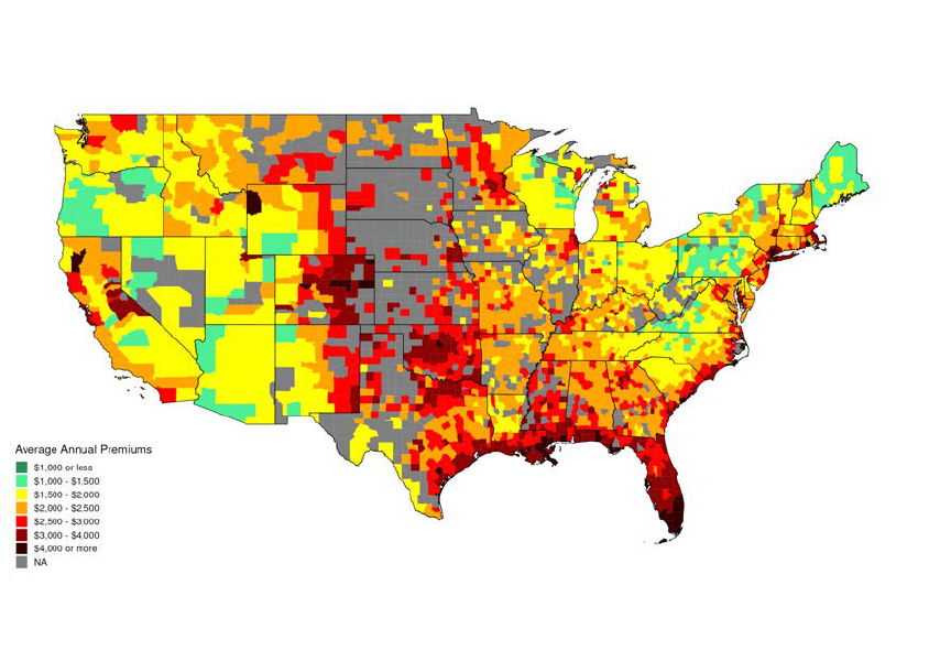
Figure 1: This ﬁgure maps average annual insurance premiums in the ﬁrst half of 2023 by county.

Counties with fewer than 20 premium observations are excluded.

separate between markets with high absolute premiums versus where premiums are placing the

largest economic burden on homeowners relative to their resources. The left panel of Figure 4 plots

average insurance premiums by zipcode income ventile. The ﬁgure shows an increasing relationship

between premiums and income, consistent with the increasing relationship between premiums and

home prices in Figure 3. In the right panel of Figure 4, we instead plot average premiums as a share

of income on the y-axis. In contrast to the left panel, this ﬁgure shows a decreasing relationship

between homeowners insurance burden and income. Moving from a zipcode with a median income

of $50,000 to a median income of $100,000 is associated with a decrease in premiums as a share of

income from 3% to 2%.

In addition to its cross-sectional richness, our data track 10 years of premium dynamics from

2014 to 2023. Figure 5 presents the time series of average nominal homeowners insurance premiums

in the United States from 2014 to 2023. Premiums were steady in nominal terms from 2014 through

2017, then rose between 2017 and 2019. Beginning in 2019, premiums leveled out until 2021. Since

2021, average premiums have risen sharply, with the average premium increasing by over $500

in three years. To investigate whether insurance costs rose faster than inﬂation over this period,

Appendix Figure 16 shows a similarly sharp increase in inﬂation-adjusted dollars.

(a) Premiums by county, 2023H1

(b) Premiums by zip code

Figure 2: This ﬁgure maps average annual insurance premiums for Southern California in the ﬁrst

half of 2023 by county (top panel) and by zipcode (bottom panel).

Figure 3: This ﬁgure shows the relationship between average premiums in 2023H1 by 20 ventiles

of home values (left panel) and the disaster risk index (right panel).

Figure 4: Figures show average premiums (left panel) and average premiums as a share of income

(right panel) by twenty ventiles of zipcode median income. Income is median income of owner-

occupied households from the 2014–2018 American Community Survey measured in 2018 dollars.

Average premiums are taken over 2014–2018 and measured in 2018 dollars.

Figure 5: Time series of nominal average annual homeowners insurance premiums.

6 Insurance Expenditure Dynamics

Having established some of the key correlates and dynamics of insurance premiums, this section

disentangles the relative inﬂuences of risk, home values, and demographics on premium diﬀerences

across space and over time. Table 4 examines the eﬀects of home values, risk, and zipcode char-

acteristics in a regression analysis. The ﬁrst column shows the bivariate relationship between real

average premiums and the IPI constructed with loan-level controls, conditional on time ﬁxed eﬀects.

A one-standard deviation increase in expected disaster losses is associated with a $450 increase in

average premiums.

Column (2) adds zipcode-level covariates for the population share white and median household

income in thousands of dollars. These covariates do little to change the estimated disaster risk

coeﬃcient. The positive relationship between incomes and insurance expenditures in consistent

with evidence that wealthier households demand more insurance (Gropper and Kuhnen, 2021;

Armantier et al., 2023). Column (2) also shows that zipcodes with higher nonwhite population

shares see higher premiums, with a 10 percentage point decrease in the white population share

associated with approximately $38 higher annual premiums. While this relationship is conditional

on home price controls and credit score controls in the IPI, disaster risk, and income, we note

that it does not hold ﬁxed other factors that may aﬀect insurers’ costs or diﬀerences in insurance

demand.

In column (3), we add state-by-year ﬁxed eﬀects to absorb time-varying factors at the state

level, such as insurance market regulations or natural disasters, that might aﬀect premiums. Here,

we see that the disaster risk coeﬃcient attenuates to a $330 premium increase with a one standard

deviation increase in disaster risk. This analysis suggests that state-level factors and diﬀerences in

home values partially, but not completely, drive the aggregate relationship between premiums and

disaster risk. Thus, our zipcode-level IPIs are critical for estimating the appropriate pass-through

of risk to premiums.

It is important to note that column (3) of Table 4 measures the eﬀect of disaster risk on

insurance spending, i.e. premiums, and not rates, or the cost per unit of coverage. This approach

is a consequence of our data, where we only observe total premiums and not the exact coverage

purchased. However, the eﬀect of risk on total insurance spending is a relevant measure of the costs

of disaster risk for households. If living in a risk-prone area leads homeowners to choose a lower

deductible or buy more coverage, then paying for that lower deductible is as much a cost of risk as

Klein and Grace (2001) study zipcode-level insurance premiums in Texas and ﬁnd that diﬀerences in premiums

by socioeconomic status can be explained by insurance demand and expected losses.

(1) (2) (3)

Insurance Premium Expenditures Index

Disaster Risk 447.822*** 495.943*** 333.540***

(15.737) (15.288) (16.357)

Pop. Share White -380.382*** -287.976***

(32.872) (35.363)

Median Income ($1000s) 12.584*** 12.764***

(0.357) (0.329)

N 177,631 177,479 177,479

R2 0.254 0.391 0.545

Demographic Controls No Yes Yes

Year#Semester FE Yes Yes Yes

Year#Semester#State FE No No Yes

* p<0.10, ** p<0.05, *** p<0.01

Table 4: Regression analysis of the determinants of insurance premiums. Observations are weighted

by ACS 2010–2014 5-year estimates of owner-occupied property counts in each zipcode, and subset

to a balanced panel of zipcodes with at least 20 observations in each period.

facing a higher rate for coverage.

A caveat to this interpretation is that diﬀerences in coverage choices driven by risk preference

heterogeneity correlated with risk do not reﬂect the cost of risk. While it is impossible to perfectly

control for such preference heterogeneity, this concern motivates the inclusion of loan-level and

zipcode-level controls as well as state-by-time ﬁxed eﬀects. On the other hand, if higher rates lead

homeowners to buy less coverage, then our measures will understate the true costs of risk and

climate change.

Table 4 assumes that the relationship between disaster risk and premiums is constant over the

sample period. To interrogate this assumption, Figure 6 shows the time series of average insurance

premium expenditures by disaster risk quintile (as measured by NRI). As reﬂected in Table 4,

disaster risk was a strong predictor of average premiums at the start of our time series in 2014,

with the riskiest quintile paying nearly double the premiums of the safest quintile. The diﬀerences

across quintiles were stable until 2020, when premiums in the riskiest quintile began to increase

sharply. Thereafter, premiums have risen across all climate risk quintiles, but the gap between

risky and safe areas has substantially widened.

This cross-sectional variation across disaster exposure in the rise of premiums suggests that

general factors – such as inﬂation, interest rates, supply chain, or labor shortages – cannot fully

explain the post-2020 rise in premiums. While the notable premium increases across all ﬁve quintiles

Leverty et al. (2023) ﬁnds a positive eﬀect of climate risk perceptions on homeowner’s insurance demand.

Figure 6: Average premiums plotted by quintile of disaster risk exposure. Premiums are in real

2023 dollars.

show that these factors likely played some role in higher premiums, the data also provide evidence

that disaster risk became a more important determinant of premiums after 2019.

To investigate the extent to which higher premiums are being driven by disaster risk exposure

versus some correlated factor, we estimate the following speciﬁcation:

IP I

zst

= α

+ α

+ β

ShareW hite

+ β

Income

+ λHomeP rice

2023H1

t=2014H2

Risk

+ ϵ

zst

, (4)

IP I

zst

is the controls insurance premium index. α

and α

are zipcode and state-by-time ﬁxed

eﬀects, respectively. We also control for population share white and median income as in column

(2) of Table 4, and for home price trends with the Zillow home value estimates (HomeP rice

The key parameters of interest are the period-by-period β

on Risk

, which give the eﬀect of a

one-standard deviation increase in disaster risk on premiums. Critically, the β

coeﬃcients are esti-

mated conditional on home price growth or other time-varying statewide factors that also aﬀected

premiums.

Figure 7 presents the time-varying coeﬃcient of climate risk on premiums from Equation 4.

While the relationship between climate risk and premiums was stable – or even decreasing – through

Figure 7: Plots the time-varying estimated eﬀect of disaster risk on premiums. Vertical lines

indicate 95% conﬁdence intervals. See Equation 4 for more details.

2019, starting in 2020 we estimate a substantially stronger relationship between premiums and

climate risk, consistent with the raw data in Figure 6. The coeﬃcient on risk increases 66% from

$300 per index unit through 2018 to nearly $500 in 2023. This increase implies a $260 increase in

annual premiums for zipcodes in the top decile of disaster risk.

To examine the robustness of our results, we re-estimate the dynamics of the risk coeﬃcient

with our repeat-loan IPI adjusted for inﬂation as the dependent variable. Because it identiﬁes

changes in premiums by following the same loan over time, it is more robust to potential biases

caused by changes in the composition of homeowners over time. The results, shown in Appendix

Figure 17, show a similar increase in the risk coeﬃcient from the base period as in the controls IPI.

7 Reinsurance and the Cost of Disaster Risk

The previous section established that the real cost of homeowners insurance has grown between

2018 and 2023, especially in areas exposed to more climate risk. Furthermore, we show that the

widening premium gap between high and low risk areas cannot be explained by statewide factors

or relative home price trends. Over this same period, catastrophe reinsurance markets hardened

substantially, raising the possibility that some of this spending increase reﬂects insurers passing

through reinsurance costs to homeowners (Eaglesham, 2024). Between 2019 and 2023 – the same

period as the risk-to-premium pass-through rose – the price of reinsurance in the U.S. Property

Catastrophe market increased by over 85% according to the Guy Carpenter Rate-On-Line Index,

Figure 8: Time series of the Guy-Carpenter U.S. Property Catastrophe Rate-on-Line Index. See

https://www.artemis.bm/us-property-cat-rate-on-line-index/ for more information.

as shown in left panel of Figure 8. Even as their prices rose, reports indicate that reinsurers also

restricted the quantity of coverage they were willing to write (Corbineau et al., 2023).

The role of reinsurance in driving premium dynamics is important for two reasons. First,

climate change is expected to exacerbate the wildﬁre and hurricane risks that form much of the

underlying risk in reinsurance contracts. Second, the eﬀect of reinsurance prices on premiums shows

how the cost of global risk intermediation aﬀects what homeowners pay to insure catastrophic risk.

However, it is an open question whether rising reinsurance prices reﬂect higher costs of homeowners

insurance everywhere, or if the cost of insuring risk is rising faster in markets that rely on reinsurers

for diversiﬁcation.

To separate the pass-through of reinsurance prices from other potential causes of rising pre-

miums in high-risk areas, we create a state-level measure of 2019 reinsurance exposure.

While

premiums ceded are not deﬁned by geography, we do know insurers’ direct premiums written in

each state. Let d

be the direct premiums written by insurer i in state s, D

s∈S

be the

total direct premiums written by i across all states, c

be the dollar value of premiums ceded by i

to unaﬃliated reinsurers, and C

be the share of i’s premiums ceded to unaﬃliated reinsurers.

We deﬁne each state’s reinsurance exposure:

We thank Ty Leverty for his help accessing this data and advice deﬁning the exposure measures.

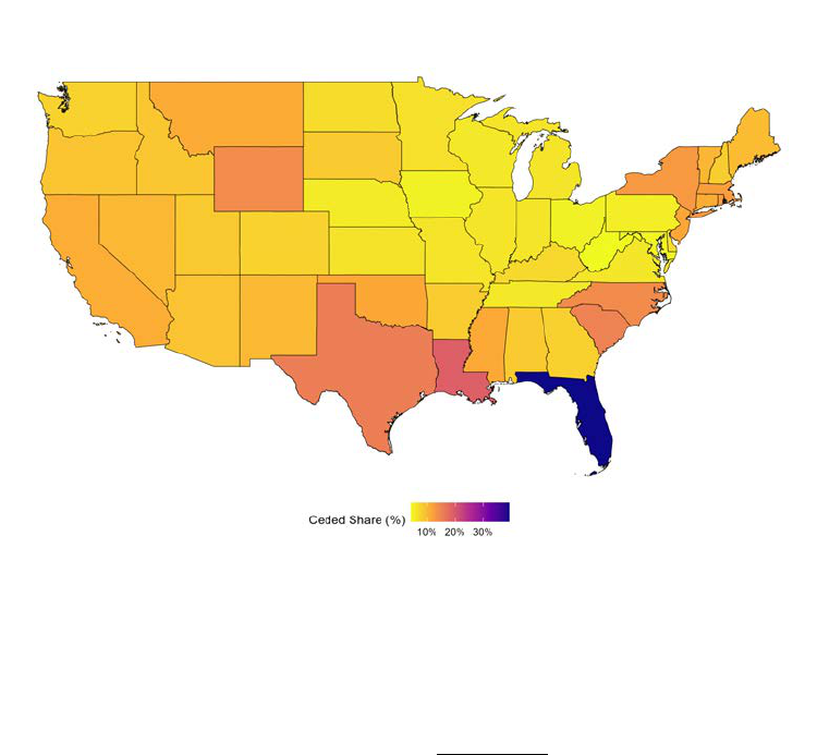
Figure 9: Map of state-level reinsurance exposure. Reinsurance exposure for each state is deﬁned

as the market-share weighted average of the share of premiums ceded by each insurer.

ReExposure

i∈I

A state’s exposure to reinsurance markets, ReExposure

, is thus the market-share weighted average

of the share of premiums ceded by each insurer. Figure 9 maps reinsurance exposure across states.

The insurers that tend to write business in riskier states – especially hurricane-exposed states –

also tend to transfer more of their risk to reinsurers, consistent with the purpose of reinsurance to

manage catastrophic risk.

Before proceeding to our econometric analysis, we compare two adjacent states with diﬀerent

reinsurance exposure: Florida, with an exposure of nearly 40%, and Georgia with an exposure of

less than 10%. Nearly all of Florida is hurricane-exposed and its property & casualty insurance

market is dominated by specialty Florida insurers, whereas Georgia has more national carriers who

rely less on reinsurance. Figure 10 plots the zipcode-level change in premiums between 2018 and

2023 along the northeast coast of Florida in St. Johns county across the border with Georgia into

McIntosh county.

Although the stretch of zipcodes along either side of the state boundary are similarly disaster-

exposed, the zipcodes in Florida saw higher premium increases between 2018 and 2023 than their

Figure 10: The real diﬀerence in annual insurance premiums between the second half of 2018 and

the ﬁrst half of 2023 for zipcodes in selected counties in Florida and Georgia. Zipcodes with fewer

than 20 loan observations in 2018H2 or 2023H1 are omitted. Dark lines indicate state and coastal

boundaries.

counterparts in Georgia.

Real premiums increased by approximately $1,000 on the Florida side

of the boundary but by less than $500 on the Georgia side.

Moving from this case study to statistical analysis, we treat the sudden increase in reinsurance

prices from 2019 to 2023 as a natural experiment. We use the following triple-diﬀerence speciﬁcation

to test the eﬀect of reinsurance rates on the pricing of disaster risk:

∆

2023H1

2018H2

IP I

= β

∆

2023H1

2018H2

HP I

+β

ReExposure

+β

Risk

+β

ReExposure

X Risk

+ϵ

, (5)

where the dependent variable, ∆

2023H1

2018H2

IP I

, is the change in the Insurance Premium Index in

inﬂation-adjusted 2023 dollars between the second half of 2018 and the ﬁrst half of 2023 in zipcode

z of state s. The independent variables are the change in zipcode z’s home values in thousands

of 2023 dollars over the same period, s’s reinsurance exposure, zipcode z’s disaster risk, and the

See Appendix Figure 14 for the associated zipcode risk measures.

(1) (2) (3) (4)

2018–2023 Premium Change (2023 Dollars)

Dependent Variable Mean: 284.93

Disaster Risk 260.445*** 13.221 70.155*** 87.797***

(16.335) (25.597) (25.427) (22.778)

ReExposure 1,644.371*** 33.971

(120.237) (151.466)

Risk X ReExposure 1,232.308*** 517.096*** 456.530***

(95.736) (106.202) (102.612)

Risk X Regulatory Friction -245.379

(197.647)

2018–2023 Home Price Change 0.843*** 0.785*** 1.312*** 1.315***

(0.194) (0.188) (0.207) (0.207)

Constant -89.474*** 97.089*** 110.316*** 108.094***

(14.167) (18.111) (15.834) (15.657)

Observations 9,336 9,336 9,336 9,336

R-squared 0.259 0.283 0.438 0.438

State FE N N Y Y

Robust standard errors in parentheses.

*** p<0.01, ** p<0.05, * p<0.1

Table 5: This table shows estimates of the pass-through of reinsurance prices to premiums. The

dependent variable is the change in the ﬁxed eﬀects insurance premium expenditures index between

2018H2 and 2023H1 by zipcode in 2023 dollars. Only zipcode observations with at least twenty

loan observations in 2018H2 and 2023H1 are included. Observations are weighted by the number

of owner-occupied housing units according to the 2010–2014 5-year American Community Survey.

See Equation 5 for details.

interaction between reinsurance exposure and disaster risk. Speciﬁcations are estimated with robust

standard errors.

The key assumption to identify β

is that the risk-to-premium relationship would have evolved

similarly in more- and less-reinsurance exposed states absent changing reinsurance prices. To lend

this assumption more credibility, we add state ﬁxed eﬀects to Equation 5 that absorb state-level

factors driving premium changes that might be correlated with reinsurance exposure. Thus, we

can identify β

from within-state variation in disaster risk.

The results of estimating Equation 5 are shown in Table 5. In column (1), we include the

reinsurance exposure and disaster risk terms without an interaction term. A $1,000 increase in

Notably, our assumption is not that the actual private cost of insuring risk remained similar across states with

diﬀerent reinsurance exposure. Rather, reinsurers likely raised their prices precisely because they perceived higher

costs of insuring in states with concentrated catastrophic risk exposure. In addition, supposing reinsurance prices

remained ﬂat is a partial equilibrium counterfactual. If reinsurance prices had been exogenously ﬁxed, it likely would

have led to an even sharper decline in reinsurance capacity.

home values is associated with about $0.84 more insurance spending, while a one-standard devi-

ation increase in disaster risk is associated with $260 higher premiums in 2023 relative to 2018.

The coeﬃcient on reinsurance exposure implies that moving from the 10th percentile to the 90th

percentile of reinsurance exposure (e.g. from Pennsylvania where insurers cede an average of 5%

of their premiums, to Texas where they cede 16% of their premiums) increases average premiums

by approximately $180.

In column (2) we add a risk-by-reinsurance exposure interaction term. Moving from column

(1) to column (2), the disaster risk term attenuates from positive and statistically signiﬁcant to

approximately null. Much of the positive eﬀect of reinsurance exposure on premiums from column

(1) is now explained by the interaction between reinsurance exposure and risk. In short, premiums

increased after 2019 for high-risk zipcodes relative to low-risk ones, but primarily in states exposed

to reinsurance.

In column (3), we apply a more stringent identiﬁcation standard to our baseline speciﬁcation

by adding state ﬁxed eﬀects. This speciﬁcation absorbs any state factors – such as idiosyncrasies

of the housing market not captured in prices, natural disasters, or insurance market regulations

– that may be correlated with reinsurance exposure and explain some of the change in premiums

around the reinsurance price shock. This speciﬁcation shows a positive and statistically signiﬁcant

risk-by-reinsurance exposure term.

To illustrate the economic signiﬁcance of our estimates, Figure 11 maps the reinsurance premium

shock by county from our estimates in column (3).

The pass-through of reinsurance costs is

extremely concentrated in disaster-prone areas in states with more reinsurance exposure. While

the median reinsurance shock across zipcodes was less than $10, zipcodes in the top decile of disaster

risk experienced average real increases of $375 from rising reinsurance rates, or over

of their total

increase in premiums between 2018 and 2023. Seven counties in Florida, collectively containing

over two million owner-occupied housing units, had reinsurance shocks of $600.

We learn several novel facts about homeowners insurance markets from the results above. While

the previous literature has documented markups and ﬂuctuations in reinsurance costs, we show

the ﬁrst evidence that those costs are largely passed through to homeowners. Second, we have

shown that the pass-through of reinsurance costs changes not just the level of premiums but the

relationship between premiums and disaster risk. Third, we show that reinsurance shocks are

In column (4) we add an interaction term between disaster risk and regulatory pricing frictions, as deﬁned in

Oh et al. (2022), reﬂecting state regulatory barriers to freely adjusting premiums. The inclusion of this regulatory

stringency measure does little to change the risk and reinsurance interaction term.

The reinsurance premium shock is deﬁned at the zipcode level as ReShock

∗ ReExposure

∗ Risk

. We

take the mean of ReShock

at the county level weighted by the number of owner-occupied housing units according

to the 2010–2014 5-year American Community Survey.

Number of owner-occupied housing units comes from July 2023 Census estimates.

Figure 11: Plots reinsurance shocks by county. Reinsurance shocks are calculated as the real dollar

increase in premiums between 2018 and 2023 caused by rising reinsurance prices.

geographically concentrated, leading to large burdens in a relatively small number of markets

rather than evenly spreading costs. In sum, insurers’ reliance on reinsurance markets combined

with an unexpected cost shock has made it more expensive to insure catastrophic risk.

8 Reinsurance and the Cost of Climate Change

The previous section detailed how recent insurance and reinsurance market dynamics have hetero-

geneously aﬀected the premiums paid by U.S. homeowners, increasing the eﬀect of disaster risk on

premiums in some states more than others. In this section, we use our forward-looking measure

of climate risk that accounts for expected changes in hurricane and wildﬁre losses to project how

homeowner’s insurance premiums will increase between 2023 and 2053.

First, we show projected premium increases due to climate change given the premium coeﬃcients

on disaster risk after the reinsurance shock. Speciﬁcally, we measure the expected increase in

premiums due to climate change:

(

Risk

2018H2

Risk

ReShock

+ ReExposure

∗

RiskXReExposure

) ∗ (Risk

2053

− Risk

2023

), (6)

where

Risk

ReShock

and

RiskXReExposure

are the estimated risk and risk-by-reinsurance exposure in-

teraction terms from column (3) of Table 5, and

Risk

2018H2

is the baseline eﬀect of disaster risk on

premiums in 2018H2 as estimated in Figure 7.

The county-level averages of these potential climate premium costs for “climate-exposed” home-

owners – those in the top 5% of expected disaster risk increase – are shown in Figure 12. On average,

this group faces annual premium increases of over $700 by 2053 due to higher disaster risk. Ex-

trapolating our full-sample estimates to the approximately 80 million single-family homes in the

U.S. implies additional annual premiums of $5.1 billion by 2053.

This analysis assumes that the risk-to-premium relationship will resemble our estimates from

2023 after the reinsurance shock increased the risk-to-premium gradient. However, to benchmark

premium changes if reinsurance prices fall, we can calculate the projected increase in premiums if

the risk-to-premium relationship reverts to its 2018 levels. Eﬀectively, we recalculate Equation 6

setting

Risk

ReShock

and

RiskXReExposure

to zero.

Figure 12: Climate Premium Shocks. This ﬁgure shows the expected increase in average annual

homeowners insurance premiums by county among households in the top 5% of expected disaster

risk increase under 2023 insurance costs.

To illustrate the inﬂuence of reinsurance costs on the premium costs of climate change, Figure

13 plots 2053 annual premium increases under 2023 (red) and 2018 (blue) insurance costs by 20

ventiles of climate exposure. Annual premium increases among climate-exposed homeowners are

only $480 under 2018 costs instead of $700 under 2023 costs, and aggregate premium increases due

to climate change are reduced by more than 30%. Premium increases are 90% higher in Florida

and 50% higher in Texas under 2023 insurance costs relative to 2018 insurance costs. Thus, our

reinsurance shock estimates show that the costs of intermediating catastrophic risk are an important

determinant of the potential costs of climate change.

Another upshot of our ﬁndings is that premium increases due to climate change will depend

on the correlation between where disaster risk is expected to increase and where insurers rely on

reinsurance markets. While the FSF model projects expected wildﬁre losses to double by 2053,

hurricane losses are only expected to increase by about 10%.

Reinsurance exposure today is

concentrated among states exposed to hurricane rather than wildﬁre risks, attenuating the projected

impact of the reinsurance shock on projected premium increases due to climate change.

The preceding analysis is subject to several caveats. First, these climate projections hold ﬁxed a

vast array of other factors between 2023 and 2053 that will also inﬂuence disaster damages. Second,

these projections only consider climate costs from the perspective of household premium payments

and do not account for insurer proﬁts or state subsidies. Third, these costs do not account for

the economic costs households face from uninsured losses. Finally, these costs reﬂect insurance

spending and not premium rates. If households reduce their coverage in response to higher rates,

premium costs will further understate climate costs.

Thus, we view these estimates as an informative baseline that suggests potential economic

responses to a changing climate as well as what factors may drive climate costs higher or lower.

Adaptation may reduce premium increases relative to our projections as building standards make

homes more resilient and spatial resorting moves population out of harms way (Bunten and Kahn,

2017; Baylis and Boomhower, 2022; Cruz and Rossi-Hansberg, 2024; Kahn et al., 2024). Continuing

cross-subsidization of risk from premium regulations and subsidized insurers-of-last-resort could,

however, blunt the incentives to adapt and increase building in disaster prone areas (Medders and

Nicholson, 2018; Oh et al., 2022).

Our results also show that climate costs are extremely sensitive to reinsurance markets. In

projecting climate costs from 2023 insurance costs, we assume that reinsurance exposure will remain

ﬁxed. Given that reinsurance exposure is correlated with catastrophic risk, we might also expect

to see this exposure increase with climate change. On the other hand, reinsurance costs have

The First Street Foundation has further detail on their wildﬁre model (https://firststreet.org/

research-library/fueling-the-flames and hurricane model (https://firststreet.org/research-library/

worsening-winds) projections. Climate change is expected to move hurricane landfalls further north along the

Mid-Atlantic. In fact, Miami-Dade county sees a modest decrease in expected hurricane losses by 2053, although it

still faces substantial increased risk due to sea level rise and ﬂooding.

risen and declined before the most recent reinsurance shock (Boyer et al., 2012). Before 2023,

reinsurance prices peaked in 2006 before declining nearly 50% to their trough in 2017 according

to the Guy Carpenter Index (Guy Carpenter, 2024). As of writing, there are already some signs

that the reinsurance market is softening in 2024 (Araullo, 2024; Howard, 2024). Even if reinsurance

prices are lower in 2053 than 2023, our ﬁndings still show that volatility in reinsurance prices create

volatility in premiums under climate change. Furthermore, it is unclear what eﬀect the increasing

frequency and severity of catastrophic risks will have on long-run reinsurance prices and capacity.

A ﬁnal implication of our ﬁndings is that reducing the frictional capital costs of insuring catas-

trophic risks is a tool to reduce the costs of climate change. Although reinsurance contracts still

represent the main conduit of global capital to U.S. insurers, growing markets in cat bonds and

other insurance linked securities may hold promise to lower the cost of ﬁnancing catastrophic risk

(Cummins et al., 2004; Braun, 2016).

Figure 13: Predicted increase in annual insurance premiums in 2053 due to climate change under

2018 insurance costs (blue) and 2023 insurance costs (red) by twenty ventiles of climate exposure.

9 Conclusion and Directions for Future Research

Property insurance serves as the front line of defense against climate risk for homeowners and

real estate investors. The cost of this insurance is a critical input into decisions to adapt or

relocate. To date, however, data limitations have hampered investigations of the geography of

homeowners insurance, the relationship between disaster risk and the price of insurance, and the

role of reinsurance markets in insurance pricing.

In this paper, we bring a new data source to bear on these critical questions. Using data from

mortgage escrow payments, we infer insurance expenditures and show that this method produces

expenditure estimates that are consistent with other publicly available sources. While the approach

has limitations, the sample size and level of detail allow for unprecedented insight into homeowners

insurance markets.

We ﬁnd that premiums have risen sharply since 2020, that this growth has been concentrated

in disaster-prone zipcodes, and that elevated reinsurance costs are a critical driver of the increase.

We provide new estimates of the elasticity of premiums with respect to climate risk, and show that

the pass-through of risk to premiums increased more than 60% between 2018 and 2023. We also

provide a new estimate of the pass-through of reinsurance costs to insurance premiums in markets

exposed to catastrophic disasters, ﬁnding that the increase in reinsurance prices can explain over

half of the increase in the relationship between premiums and risk. The reinsurance shock added

$375 to the 2023 annual homeowners insurance premiums of households in the top decile of disaster

risk.

Our results also benchmark potential increases in premiums that climate-exposed homeowners

will face due to increasing risk. By 2053, we estimate that climate-exposed homeowners will be

paying $700 higher annual premiums due to increasing wildﬁre and hurricane risk. However, these

premium increases are highly sensitive to reinsurance prices. If insurance costs revert to their 2018

levels, then premium increases will be reduced by

. Thus, the costs of climate change depend on

the cost of accessing reinsurance markets to diversify catastrophic risks.

In subsequent research, we intend to use this large panel dataset of insurance expenditures

to examine whether insurance costs are capitalized into house prices; how rising user costs of

homeownership aﬀect mobility and housing tenure choice; the consequences of increased insurance

burdens on mortgage default; and the impact of insurer exit and growing dependence on state-

mandated FAIR plans on insurance spending. We anticipate that this data eﬀort is only an initial

foray into measuring homeowners insurance markets, and that additional data availability on policy

coverage, deductibles, and claims will be valuable for researchers, policymakers, and households that

must navigate an increasingly challenging property insurance landscape.

References

Anand, V., J. Tyler Leverty, and K. Wunder (2021). Paying for expertise: The eﬀect of experience

on insurance demand. Journal of Risk and Insurance 88 (3), 727–756.

Araullo, K. (2024). January 1 renewals reﬂect a responsive reinsurance market – guy carpenter.

Insurance Business Magazine.

Armantier, O., J. Foncel, and N. Treich (2023). Insurance and portfolio decisions: Two sides of the

same coin? Journal of Financial Economics 148(3), 201–219.

Bakkensen, L. A. and L. Barrage (2021, 11). Going Underwater? Flood Risk Belief Heterogeneity

and Coastal Home Price Dynamics. The Review of Financial Studies. hhab122.

Baldauf, M., L. Garlappi, and C. Yannelis (2020). Does climate change aﬀect real estate prices?

only if you believe in it. The Review of Financial Studies 33 (3), 1256–1295.

Bauer, D., R. Phillips, and G. Zanjani (2023). Pricing insurance risk: reconciling theory and

practice. Handbook of Insurance.

Bauer, D., L. Powell, B. Su, and G. H. Zanjani (2021). Life insurance and annuity pricing during

the ﬁnancial crisis, revisited. Revisited (March 6, 2021).

Baylis, P. W. and J. Boomhower (2022). Mandated vs. voluntary adaptation to natural disasters:

The case of us wildﬁres. Technical report, National Bureau of Economic Research.

Bernstein, A., M. T. Gustafson, and R. Lewis (2019). Disaster on the horizon: The price eﬀect of

sea level rise. Journal of ﬁnancial economics 134 (2), 253–272.

Bhutta, N. and B. J. Keys (2022). Moral hazard during the housing boom: Evidence from private

mortgage insurance. The Review of Financial Studies 35(2), 771–813.

Blickle, K. and J. A. Santos (2022). Unintended consequences of. FRB of New York Staﬀ Re-

port (1012).

Boomhower, J., M. Fowlie, J. Gellman, and A. J. Plantinga (2024). How are insurance markets

adapting to climate change? risk selection and regulation in the market for homeowners insur-

ance.

Born, P. and W. K. Viscusi (2006). The catastrophic eﬀects of natural disasters on insurance

markets. Journal of risk and Uncertainty 33, 55–72.

Boyer, M. M., E. Jacquier, and S. Van Norden (2012). Are underwriting cycles real and forecastable?

Journal of Risk and Insurance 79 (4), 995–1015.

Braun, A. (2016). Pricing in the primary market for cat bonds: new empirical evidence. Journal

of Risk and Insurance 83(4), 811–847.

Brunnermeier, M., E. Farhi, R. S. Koijen, A. Krishnamurthy, S. C. Ludvigson, H. Lustig, S. Nagel,

and M. Piazzesi (2021). Perspectives on the future of asset pricing. The review of ﬁnancial

studies 34 (4), 2126–2160.

Bunten, D. and M. E. Kahn (2017). Optimal real estate capital durability and localized climate

change disaster risk. Journal of Housing Economics 36, 1–7.

Contat, J., C. Hopkins, L. Mejia, and M. Suandi (2024). When climate meets real estate: A survey

of the literature. Real Estate Economics.

Corbineau, G., E. Fayad, D. Grunebaum, T. Lindeman, D. Reed, S. Hibler, and J. DeMarkey

(2023). Reinsurers defend against rising tide of natural catastrophe losses, for now. Moody’s.

Cruz, J.-L. and E. Rossi-Hansberg (2024). The economic geography of global warming. Review of

Economic Studies 91(2), 899–939.

Cummins, J. D., G. Dionne, R. Gagn´e, and A. Nouira (2021). The costs and beneﬁts of reinsurance.

The Geneva Papers on Risk and Insurance-Issues and Practice 46, 177–199.

Cummins, J. D., D. Lalonde, and R. D. Phillips (2004). The basis risk of catastrophic-loss index

securities. Journal of Financial Economics 71 (1), 77–111.

Cummins, J. D. and M. A. Weiss (2009). Convergence of insurance and ﬁnancial markets: Hybrid

and securitized risk-transfer solutions. Journal of Risk and Insurance 76 (3), 493–545.

Eaglesham, J. (2024). The hidden driver of soaring home insurance costs. Wall Street Journal.

Eastman, E. and K. Kim (2023). Regulatory capital and catastrophe risk. Available at SSRN

4468543 .

FEMA (2023). National risk index. https://hazards.fema.gov/nri/learn-more.

First Street Foundation (2020). https://firststreet.org.

Froot, K. A. (2001). The market for catastrophe risk: a clinical examination. Journal of Financial

Economics 60 (2-3), 529–571.

Froot, K. A. (2007). Risk management, capital budgeting, and capital structure policy for insurers

and reinsurers. Journal of risk and Insurance 74 (2), 273–299.

Froot, K. A., B. Murphy, A. Stern, S. Usher, et al. (1995). The emerging asset class: insurance

risk. A Special Report From Guy Carpenter & Company, Inc.

Froot, K. A. and P. G. O’Connell (1999). The pricing of us catastrophe reinsurance. In The

ﬁnancing of catastrophe risk, pp. 195–232. University of Chicago Press.

Froot, K. A. and P. G. O’Connell (2008). On the pricing of intermediated risks: Theory and

application to catastrophe reinsurance. Journal of Banking & Finance 32 (1), 69–85.

Gallagher Re (2024). First view. Technical report.

Ge, S. (2022). How do ﬁnancial constraints aﬀect product pricing? evidence from weather and life

insurance premiums. The Journal of Finance 77(1), 449–503.

Ge, S., A. Lam, and R. Lewis (2022). The costs of hedging disaster risk and home prices: Evidence

from ﬂood insurance. Available at SSRN .

Georgic, W. and H. A. Klaiber (2022). Stocks, ﬂows, and ﬂood insurance: A nationwide analysis of

the capitalized impact of annual premium discounts on housing values. Journal of Environmental

Economics and Management 111, 102567.

Government Accountability Oﬃce (2021). National ﬂood insurance program: Congress should

consider updating the mandatory purchase requirement. Technical report.

Gron, A. (1994). Capacity constraints and cycles in property-casualty insurance markets. The

RAND Journal of Economics, 110–127.

Gron, A. (1999). Insurer demand for catastrophe reinsurance. In The ﬁnancing of catastrophe risk,

pp. 23–50. University of Chicago Press.

Gron, A. and D. J. Lucas (1995). External ﬁnancing and insurance cycles.

Gropper, M. J. and C. M. Kuhnen (2021). Wealth and insurance choices: Evidence from us

households. Technical report, National Bureau of Economic Research.

Guy Carpenter (2024). Guy carpenter index. https://www.guycarp.com/insights/2024/01/

global-rate-on-line-index-2000-2024.html.

Harrington, S. E. (2004). Tort liability, insurance rates, and the insurance cycle. Brookings-Wharton

Papers on Financial Services 2004 (1), 97–138.

Howard, L. (2024). Reinsurance market likely to begin softening in 2025 as capacity rises in 2024:

Fitch. Insurance Journal.

Ibragimov, R., D. Jaﬀee, and J. Walden (2009). Nondiversiﬁcation traps in catastrophe insurance

markets. The Review of Financial Studies 22 (3), 959–993.

Insurance Information Institute (2024). Facts + statistics: Homeowners and renters insurance.

Issler, P., R. Stanton, C. Vergara-Alert, and N. Wallace (2020). Mortgage markets with climate-

change risk: Evidence from wildﬁres in california. Available at SSRN 3511843 .

Jaﬀee, D. M. and T. Russell (1997). Catastrophe insurance, capital markets, and uninsurable risks.

Journal of Risk and Insurance, 205–230.

Jeziorski, W. and S. Ramnath (2021). Homeowners insurance and climate change. Chicago Fed

Letter (460), 1–6.

Kahn, M. E., A. Ouazad, and E. Y¨onder (2024). Adaptation using ﬁnancial markets: Climate risk

diversiﬁcation through securitization. Technical report, National Bureau of Economic Research.

Keys, B. J. and P. Mulder (2020). Neglected no more: Housing markets, mortgage lending, and

sea level rise. Technical report, National Bureau of Economic Research.

Klein, R. W. and M. F. Grace (2001). Urban homeowners insurance markets in texas: A search

for redlining. Journal of Risk and Insurance, 581–613.

Koijen, R. S. and M. Yogo (2015). The cost of ﬁnancial frictions for life insurers. American

Economic Review 105 (1), 445–475.

Koijen, R. S. and M. Yogo (2016). Shadow insurance. Econometrica 84(3), 1265–1287.

Kousky, C. and R. M. Cooke (2009). The unholy trinity: fat tails, tail dependence, and micro-

correlations. Resources for the Future Discussion Paper, 09–36.

Kousky, C., H. Kunreuther, B. Lingle, and L. Shabman (2018). The emerging private residential

ﬂood insurance market in the united states. Wharton Risk Management and Decision Processes

Center.

Kousky, C., M. Palim, and Y. Pan (2020). Flood damage and mortgage credit risk: A case study

of hurricane harvey. Journal of Housing Research 29 (sup1), S86–S120.

Leverty, J. T., T. Sun, and H. Zou (2023). Do households respond to climate change? evidence

from the us homeowners insurance market. Evidence from the US Homeowners Insurance Market

(September 7, 2023).

Lewis, R. (2023). The value of climate hedge assets: Evidence from australian water markets.

Marcoux, K. and K. R. H. Wagner (2023). Fifty years of us natural disaster insurance policy.

Medders, L. A. and J. E. Nicholson (2018). Evaluating the public ﬁnancing for ﬂorida’s wind risk.

Risk Management and Insurance Review 21 (1), 117–139.

Missouri Census Data Center (2014). Mable geographic database. http://mcdc.missouri.edu/

applications/geocorr.html.

Mulder, P. (2023). Mismeasuring risk: The welfare eﬀects of ﬂood risk information. Technical

report, Working Paper.

Murﬁn, J. and M. Spiegel (2020). Is the risk of sea level rise capitalized in residential real estate?

The Review of Financial Studies 33 (3), 1217–1255.

NAIC (2022). A consumer’s guide to home insurance.

Nyce, C., R. E. Dumm, G. S. Sirmans, and G. Smersh (2015). The capitalization of insurance

premiums in house prices. Journal of Risk and Insurance 82 (4), 891–919.

Oh, S., I. Sen, and A.-M. Tenekedjieva (2022). Pricing of climate risk insurance: Regulation and

cross-subsidies. Available at SSRN 3762235 .

Ostriker, A. and A. Russo (2022). The eﬀects of ﬂoodplain regulation on housing markets. URL

https://ostriker. github. io/papers/Ostriker-Russo ﬂoodplain-regulations. pdf .

Ouazad, A. and M. E. Kahn (2021, 11). Mortgage Finance and Climate Change: Securitization

Dynamics in the Aftermath of Natural Disasters. The Review of Financial Studies. hhab124.

Panjwani, A. (2022). Underwater: The eﬀect of federal policies on households’ exposure to climate

change risk. Technical report, Working paper.

Poterba, J. M. (1984). Tax subsidies to owner-occupied housing: an asset-market approach. The

quarterly journal of economics 99(4), 729–752.

Sastry, P. (2021). Who bears ﬂood risk? evidence from mortgage markets in ﬂorida.

Sastry, P., I. Sen, and A.-M. Tenekedjieva (2023). When insurers exit: Climate losses, fragile

insurers, and mortgage markets. Fragile Insurers, and Mortgage Markets (December 23, 2023).

Swiss Re (2024). Sigma 01/2024. Technical report.

Wagner, K. R. (2022). Adaptation and adverse selection in markets for natural disaster insurance.

American Economic Journal: Economic Policy 14 (3), 380–421.

Weill, J. (2022). Perilous ﬂood risk assessments. Available at SSRN 4143914 .

Zanjani, G. (2002). Pricing and capital allocation in catastrophe insurance. Journal of ﬁnancial

economics 65 (2), 283–305.

10 Appendix

10.1 Appendix Figures and Tables

Figure 14: Map of US zipcodes by risk measure quintile

Figure 15: Shows average annual homeowners insurance premiums by zipcode in Miami-Dade

County in the ﬁrst half of 2023.

Figure 16: Time series of average annual homeowners insurance premiums. Values are inﬂated to

constant 2023 dollars.

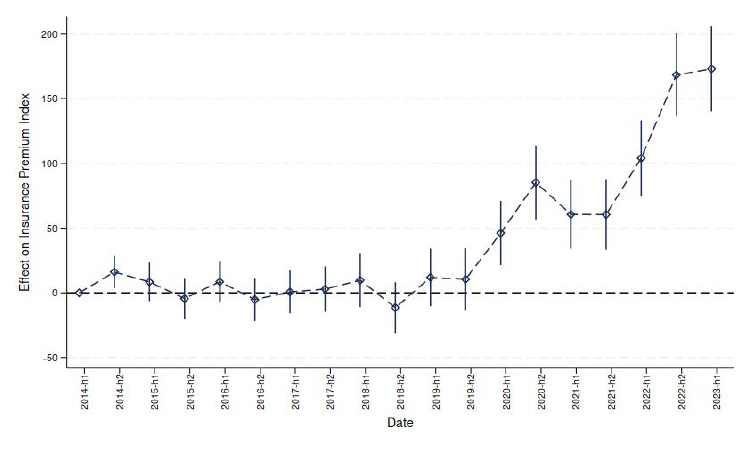
Figure 17: Plots the time-varying estimated eﬀect of disaster risk on premiums. Dependent variable

is the repeat-loan insurance premium expenditures index.

10.2 Comparison to III, Census, and Quadrant

Figure 18 compares the average nominal premiums calculated using our escrow approach with

three alternative measures, from Insurance Information Institute at the state level (III), the Census

American Community Survey (ACS) at the county-level, and from Quadrant Information Services

at the zipcode level.

Looking at the comparison with III, we see a strong and approximately one-to-one relationship

between the escrow premium estimates and the III premium estimates.

However, the escrow

estimates are consistently about $500 more expensive than their corresponding III ﬁgures. We

consider several potential explanations for this. First, our estimates consider whatever premiums

homeowners pay out of escrow, including ﬂood insurance policies, policies outside the standard

HO-3 coverage, or supplemental wind-only or ﬁre-only coverage. The III numbers, on the other

hand focus on standard HO-3 policies. Second, the property values of our sample of mortgaged

homeowners are about 15% higher than the corresponding Zillow home value estimates.

We see a similarly strong linear relationship between the escrow premium estimates and sur-

veyed homeowners insurance premiums for the ACS and a similar upward level shift in the escrow

estimates. However, the gap between escrow and ACS premiums is larger at the top-end of the

premium distribution. We believe this gap can be explained by the fact that reported disaster

insurance premiums in the ACS are top-coded at $10,000.

Finally, we compare our premiums against price quotes from Quadrant in Florida, Louisiana,

Texas, and California. Quadrant’s data is unique in that it matches the zipcode granularity of the

the escrow estimates. However, it comes from estimated insurer prices based on their state rate

ﬁlings for standardized amounts of coverage rather than reﬂecting the actual premiums paid for

purchased coverage. There is a weaker positive relationship between escrow premium estimates and

the Quadrant price quotes relative to the III and ACS estimates. In particular, among zipcodes

with the highest average Quadrant quotes, the escrow premium estimates are substantially lower.

We believe this pattern plausibly reﬂects the shopping behavior of households, their downward

sloping demand for insurance, and unobserved coverage denials by insurers. Where Quadrant sees

some insurers setting the highest premiums, homeowners are most likely to shop and ﬁnd the lowest

premium available to them. In addition, the insurers setting the highest premiums may also be the

most likely to deny coverage. It is also relevant that, whereas the Quadrant data compare prices

across a ﬁxed contract, homeowners may choose higher deductibles or buy less coverage when facing

higher rates. Although Quadrant data provides valuable insight into the rates set by insurers, it

does not show the premiums actually paid by homeowners as in the escrow estimates.

In sum, the escrow premium estimates have a strong and positive relationship with coarser

existing datasets on homeowners insurance premiums. The escrow premiums are a level shift

higher than other sources, a fact that can be primarily explained by the more valuable homes in

our sample and that escrow payments likely cover a broader range of policies.

III premium tables are provided here: https://www.iii.org/table-archive/21407.

(a) III

(b) ACS

Figure 18: Escrow Premium Estimates versus other sources. Each ﬁgure compares the average

premiums from the escrow estimates against diﬀerent sources in the form of a binscatter. Panel (a)

compares state-by-year premium estimates between 2014 and 2020 from the Insurance Information

Institute. Panel (b) compares county-by-year premium estimates between 2014 and 2022 from the

American Community Survey. Panel (c) compares zipcode-by-year insurer cost quotes between

2014 and 2021 from Quadrant Information Services in Florida, Louisiana, California, and Texas.

Cost quotes are averaged within each zipcode by insurer, level of coverage (250K or 500K), credit

score (excellent, good, fair, or poor where applicable) and home age (new, 10 years old, 25 years

old). Quadrant rates are representative of publicly sourced data and should not be interpreted as

bindable quotes.