PowerPoint Presentation

Deep dive and best

practices for Amazon Redshift

A N T 4 1 8

Tony Gibbs

Sr. Database Specialist SA

Amazon Web Services

Harshida Patel

Data Warehouse Specialist SA

Amazon Web Services

Are you an Amazon Redshift user?

Agenda

• Architecture and concepts

• Data storage, ingestion, and ELT

• Workload management and query monitoring rules

• Cluster sizing and resizing

• Amazon Redshift Advisor

• Additional resources

• Open Q&A

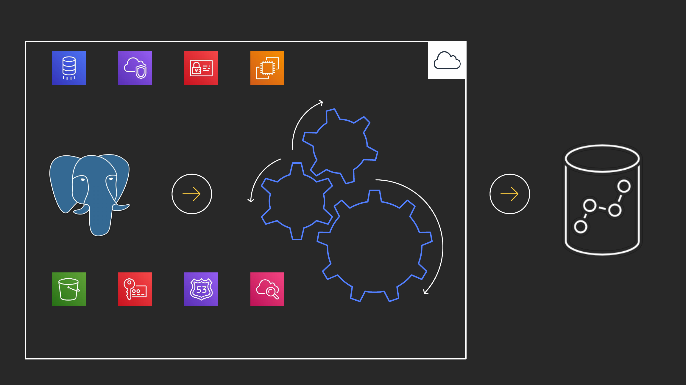
PostgreSQL

Columnar

MPP

OLAP

AWS Identity

and Access

Management

(IAM)

Amazon

VPC

Amazon

Simple

Workflow

Service

Amazon Simple

Storage

Service (S3)

AWS Key

Management

Service

Amazon

Route 53

Amazon

CloudWatch

Amazon

EC2

Amazon Redshift

AWS Cloud

February 2013

December 2019

>175 significant patches

Robust result set

caching

Large # of tables support

~20000

Copy command support

for ORC, Parquet

IAM role chaining

Elastic resize Groups

Amazon Redshift Spectrum: Date

formats, scalar json and ION file

formats support, region expansion,

predicate filtering

Auto

analyze

Health and performance

monitoring w/Amazon

CloudWatch

Automatic table

distribution style

Amazon

CloudWatch

support for

WLM queues

Performance enhancements: Hash

join, vacuum, window functions,

resize ops, aggregations, console,

union all, efficient compile

code cache

Unload

to CSV

Auto WLM

~25 Query Monitoring

Rules (QMR) support

200+

new features and

enhancements in the past

18 months

AQUA

Concurrency Scaling

DC1 migration to DC2

Resiliency of

ROLLBACK processing

Manage multi-part

query in AWS console

Auto analyze for

incremental changes

on table

Spectrum Request

Accelerator

Apply new

distribution key

Redshift Spectrum: Row

group filtering in Parquet

and ORC, nested data

support, enhanced VPC

routing, multiple partitions

Faster Classic

resize with

optimized data

transfer protocol

Performance: Bloom filters in

joins, complex queries that

create internal table,

communication layer

Amazon Redshift

Spectrum:

Concurrency scaling

AWS Lake Formation

integration

Auto-Vacuum sort,

Auto-Analyze, and

Auto Table Sort

Auto WLM with

query priorities

Snapshot scheduler

Performance: Join

pushdowns to subquery,

mixed workloads temporary

tables, rank functions, null

handling in join, single row insert

Advisor recommendations

for distribution keys

AZ64 compression

encoding

Console

redesign

Stored procedures

Spatial processing Column level access

control with AWS Lake

Formation

RA3

Performance of

inter-region snapshot

transfers

Federated

query

Materialized

views

Manual pause

and resume

Amazon Redshift has been innovating quickly

Load

Unload

Backup

Restore

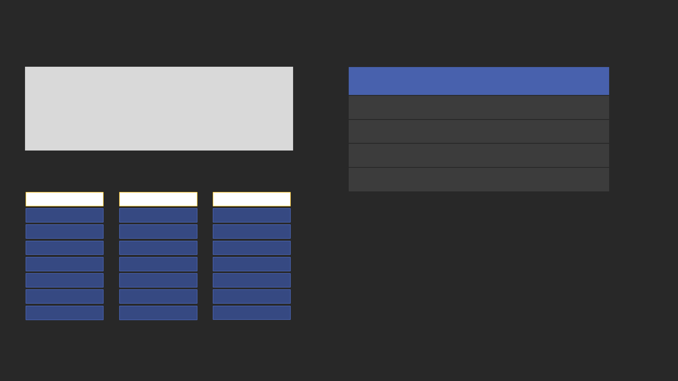
Amazon Redshift architecture

Massively parallel, shared

nothing columnar architecture

Leader node

SQL endpoint

Stores metadata

Coordinates parallel SQL processing

Compute nodes

Local, columnar storage

Executes queries in parallel

Load, unload, backup, restore

Amazon Redshift Spectrum nodes

Execute queries directly against

Amazon Simple Storage Service (Amazon S3)

SQL clients/BI tools

JDBC/ODBC

Compute

node

Compute

node

Compute

node

Leader

node

Amazon S3

...

1 2 3 4 N

Amazon

Redshift

Spectrum

Load

Query

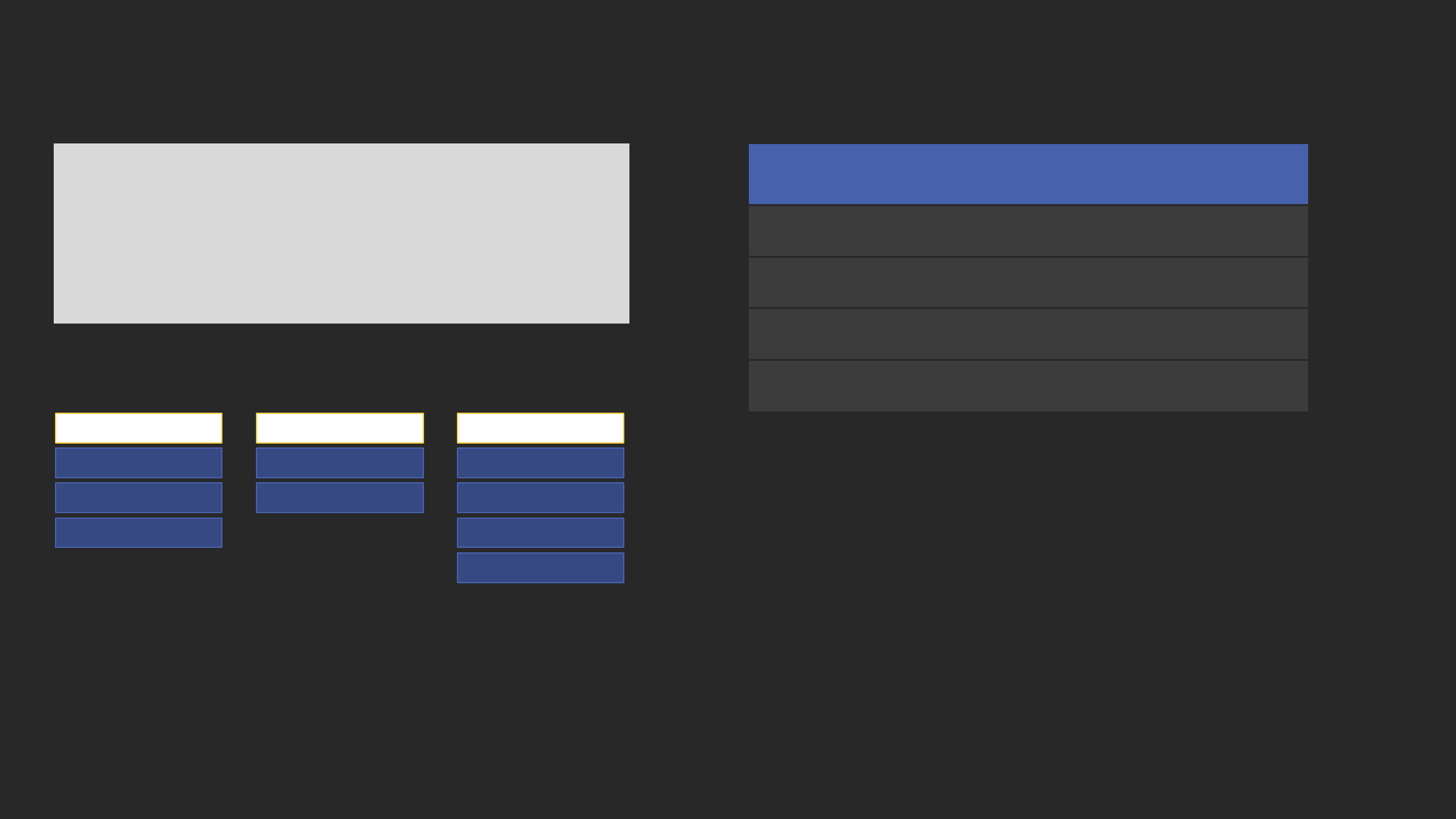
Amazon Redshift evolving architecture

SQL clients/BI tools

JDBC/ODBC

Compute

node

Compute

node

Compute

node

Leader

node

Massively parallel, shared nothing

columnar architecture

Leader node

Compute nodes

Amazon Redshift Spectrum nodes

Amazon Redshift Managed Storage

Pay separately for storage and compute

Large high-speed SSD backed cache

Automatic scaling (up to 64 TB/instance)

Supports up to 8.2 PB of cluster storage

Compute

Clusters

Compute

Clusters

Compute

Clusters

Compute

Clusters

AQUA (Advanced Query Accelerator) for Amazon Redshift

Redshift

Cluster

AQUA

node

AQUA

node

AQUA

node

AQUA

node

Amazon Redshift Managed Storage

Compute

Clusters

Compute

Clusters

Compute

Clusters

Compute

Clusters

Redshift

Cluster

Compute

Clusters

Compute

Clusters

Compute

Clusters

Compute

Clusters

Redshift

Cluster

New distributed & hardware-accelerated

processing layer

With AQUA, Amazon Redshift is up to

10x faster than any other cloud data warehouse,

no extra cost

AQUA Nodes with custom AWS-designed

analytics processors to make operations

(compression, encryption, filtering, and

aggregations) faster than traditional CPUs

Available in Preview with RA3. No code changes

required

Terminology and concepts: Node types

Amazon Redshift analytics—RA3 (new)

Amazon Redshift Managed Storage (RMS)—Solid-state disks + Amazon S3

Dense compute—DC2

Solid-state disks

Dense storage—DS2

Magnetic disks

Instance type

Disk

type

Size

Memory

CPUs

Slices

RA3 4xlarge (coming soon) RMS Scales to 16 TB 96 GB 12 4

RA3 16xlarge (new) RMS Scales to 64 TB 384 GB 48 16

DC2 large SSD 160 GB 16 GB 2 2

DC2 8xlarge SSD 2.56 TB 244 GB 32 16

DS2 xlarge Magnetic 2 TB 32 GB 4 2

DS2 8xlarge Magnetic 16 TB 244 GB 36 16

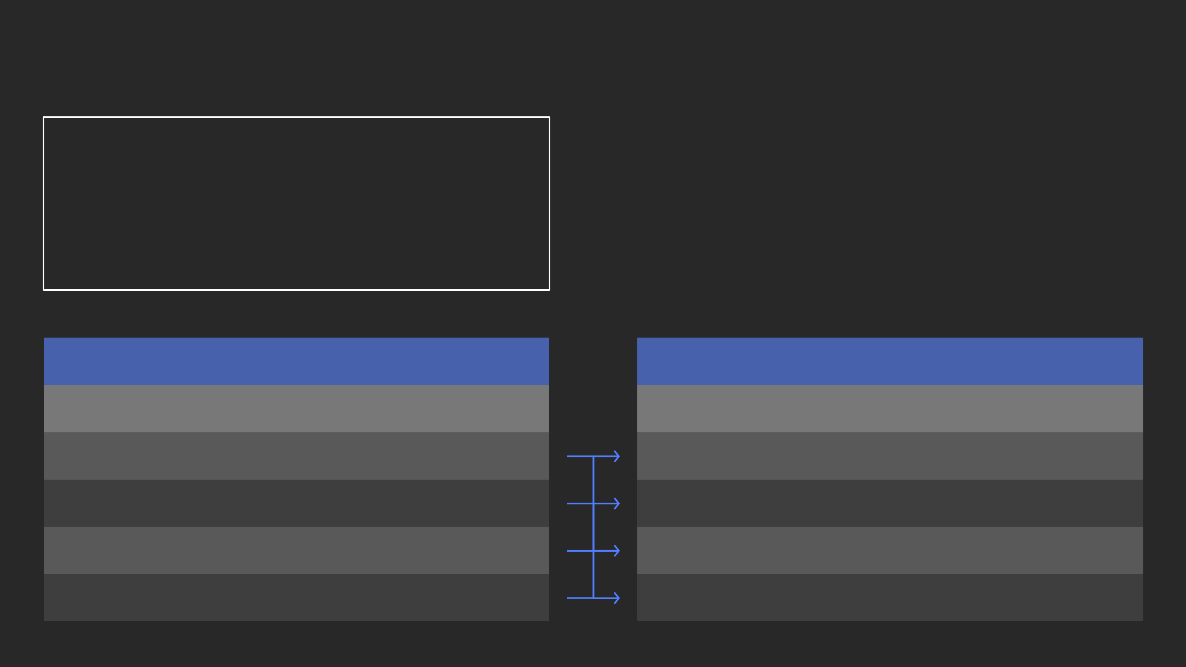
Terminology and concepts: Columnar

Amazon Redshift uses a columnar architecture for storing data on disk

Goal: reduce I/O for analytics queries

Physically store data on disk by column rather than row

Only read the column data that is required

Row-based storage

• Need to read everything

• Unnecessary I/O

aid loc dt

CREATE TABLE deep_dive (

aid INT --audience_id

,loc CHAR(3) --location

,dt DATE --date

);

aid loc dt

1 SFO 2017-10-20

2 JFK 2017-10-20

3 SFO 2017-04-01

4 JFK 2017-05-14

SELECT min(dt) FROM deep_dive;

Columnar architecture: Example

Column-based storage

• Only scan blocks for

relevant column

aid loc dt

CREATE TABLE deep_dive (

aid INT --audience_id

,loc CHAR(3) --location

,dt DATE --date

);

aid loc dt

1 SFO 2017-10-20

2 JFK 2017-10-20

3 SFO 2017-04-01

4 JFK 2017-05-14

SELECT min(dt) FROM deep_dive;

Columnar architecture: Example

Terminology and concepts: Compression

Goals

Allow more data to be stored within

an Amazon Redshift cluster

Improve query performance by

decreasing I/O

Impact

Allows two to four times more data

to be stored within the cluster

By default, COPY automatically analyzes and compresses data on first load

into an empty table

ANALYZE COMPRESSION is a built-in command that will find the optimal

compression for each column on an existing table

Compression: Example

Add 1 of 13 different encodings

to each column

aid loc dt

CREATE TABLE deep_dive (

aid INT --audience_id

,loc CHAR(3) --location

,dt DATE --date

);

aid loc dt

1 SFO 2017-10-20

2 JFK 2017-10-20

3 SFO 2017-04-01

4 JFK 2017-05-14

Compression: Example

More efficient compression is due

to storing the same data type in

the columnar architecture

Columns grow and shrink

independently

Reduces storage requirements

Reduces I/O

aid loc dt

CREATE TABLE deep_dive (

aid INT ENCODE AZ64

,loc CHAR(3) ENCODE BYTEDICT

,dt DATE ENCODE RUNLENGTH

);

aid loc dt

1 SFO 2017-10-20

2 JFK 2017-10-20

3 SFO 2017-04-01

4 JFK 2017-05-14

AZ64 storage savings

AZ64 performance speed ups

RAW

–70% less storage

–30% faster

LZO

35% less storage

40% faster

ZSTD

Comparable footprint

70% faster

New Amazon Redshift encoding type: AZ64

AZ64 is Amazon's proprietary compression encoding algorithm designed

to achieve a high compression ratio and improved query processing

Goals:

Increase compression ratio, reducing the required footprint

Increase query performance by decreasing both encoding/decoding times

30TB Cloud DW benchmark is based on TPC-DS (v2.10) with no query modifications done

Result:

Best practices: Compression

Apply compression to all tables

In most cases, use AZ64 for INT, SMALLINT, BIGINT, TIMESTAMP, TIMESTAMPTZ, DATE, NUMERIC

In most cases, use LZO/ZSTD for VARCHAR and CHAR

Use ANALYZE COMPRESSION command to find optimal compression

RAW (no compression) for sparse columns and small tables

Changing column encoding requires a table rebuild

https://github.com/awslabs/amazon-redshift utils/tree/master/src/ColumnEncodingUtility

Verifying columns are compressed:

SELECT "column", type, encoding FROM pg_table_def

WHERE tablename = 'deep_dive';

column | type | encoding

--------+--------------+----------

aid | integer | az64

loc | character(3) | bytedict

dt | date | runlength

Terminology and concepts: Blocks

Column data is persisted to 1 MB immutable blocks

Blocks are individually encoded with 1 of 13 encodings

A full block can contain millions of values

Terminology and concepts: Zone maps

Goal

Eliminates unnecessary I/O

In-memory block metadata

Contains per-block min and max values

All blocks automatically have zone maps

Effectively prunes blocks that cannot contain data for a given query

Terminology and concepts: Data sorting

Goal

Make queries run faster by increasing

the effectiveness of zone maps and

reducing I/O

Impact

Enables range-restricted scans

to prune blocks by leveraging

zone maps

Achieved with the table property

SORTKEY defined on one or more columns

Optimal sort key is dependent on:

Query patterns

Business requirements

Data profile

CREATE TABLE deep_dive (

aid INT --audience_id

,loc CHAR(3) --location

,dt DATE --date

)

SORTKEY (dt, loc);

Sort key: Example

Add a sort key to one or more

columns to physically sort

the data on disk

deep_dive

aid loc dt

1 SFO 2017-10-20

2 JFK 2017-10-20

3 SFO 2017-04-01

4 JFK 2017-05-14

deep_dive (sorted)

aid loc dt

3 SFO 2017-04-01

4 JFK 2017-05-14

2 JFK 2017-10-20

1 SFO 2017-10-20

deep_dive (sorted)

aid loc dt

3 SFO 2017-04-01

4 JFK 2017-05-14

2 JFK 2017-10-20

deep_dive (sorted)

aid loc dt

3 SFO 2017-04-01

4 JFK 2017-05-14

deep_dive (sorted)

aid loc dt

3 SFO 2017-04-01

SELECT count(*) FROM deep_dive WHERE dt = '06-09-2017';

MIN: 01-JUNE-2017

MAX: 06-JUNE-2017

MIN: 07-JUNE-2017

MAX: 12-JUNE-2017

MIN: 13-JUNE-2017

MAX: 21-JUNE-2017

MIN: 21-JUNE-2017

MAX: 30-JUNE-2017

Sorted by date

MIN: 01-JUNE-2017

MAX: 20-JUNE-2017

MIN: 08-JUNE-2017

MAX: 30-JUNE-2017

MIN: 12-JUNE-2017

MAX: 20-JUNE-2017

MIN: 02-JUNE-2017

MAX: 25-JUNE-2017

Unsorted table

Zone maps and sorting: Example

Best practices: Sort keys

Place the sort key on columns that are frequently filtered on placing

the lowest cardinality columns first

On most fact tables, the first sort key column should be a temporal column

Columns added to a sort key after a high-cardinality column are not effective

With an established workload, use the following scripts to help find

sort key suggestions:

https://github.com/awslabs/amazon-redshift-utils/blob/master/src/AdminScripts/filter_used.sql

https://github.com/awslabs/amazon-redshift-

utils/blob/master/src/AdminScripts/predicate_columns.sql

Design considerations:

Sort keys are less beneficial on small tables

Define four or less sort key columns—more will result in marginal gains

and increased ingestion overhead

Terminology and concepts: Materialize columns

Goal: Make queries run faster by leveraging zonemaps on the fact tables

Frequently filtered and unchanging dimension values should be materialized within fact tables

Time dimension tables do not allow for range restricted scans on fact tables

Materializing temporal values in fact table can give significant performance gains

Example:

SELECT COUNT(*) FROM fact_dd JOIN dim_dd USING (timeid) WHERE dim_dd.ts >= '2018-11-29';

SELECT COUNT(*) FROM fact_dd WHERE fact_dd.timestamp >= '2018-11-29’; -- Faster

Often calculated values should be materialized within fact tables

Example:

SELECT COUNT(*) FROM dd WHERE EXTRACT(EPOCH FROM ts) BETWEEN 1541120959 AND 1543520959;

SELECT COUNT(*) FROM dd WHERE sorted_epoch BETWEEN 1541120959 AND 1543520959; -- Faster

Terminology and concepts: Slices

A slice can be thought of

like a virtual compute node

Unit of data partitioning

Parallel query processing

Facts about slices

Each compute node is initialized with either 2

or 16 slices

Table rows are distributed to slices

A slice processes only its own data

Data distribution

Distribution style is a table property which

dictates how that table’s data is distributed

throughout the cluster

KEY: Value is hashed, same value goes to same location (slice)

ALL: Full table data goes to the first slice of every node

EVEN: Round robin

AUTO: Combines EVEN and ALL

Goals

Distribute data evenly for

parallel processing

Minimize data movement

during query processing

KEY

Node 1

Slice

Node 2

Slice

ALL

Node 1

Slice

Node 2

Slice

EVEN

Node 1

Slice

Node 2

Slice

Node 1

Data distribution: Example

Slice 0 Slice 1

Node 2

Slice 2 Slice 3

Table: deep_dive

User columns System columns

aid loc dt ins del row

CREATE TABLE deep_dive (

aid INT --audience_id

,loc CHAR(3) --location

,dt DATE --date

) (EVEN|KEY|ALL|AUTO);

Node 1

Slice 0 Slice 1

Node 2

Slice 2 Slice 3

Data distribution: EVEN Example

INSERT INTO deep_dive VALUES

(1, 'SFO', '2016-09-01'),

(2, 'JFK', '2016-09-14'),

(3, 'SFO', '2017-04-01'),

(4, 'JFK', '2017-05-14');

Table: deep_dive

User Columns System Columns

aid loc dt ins del row

Table: deep_dive

User Columns System Columns

aid loc dt ins del row

Table: deep_dive

User Columns System Columns

aid loc dt ins del row

Table: deep_dive

User Columns System Columns

aid loc dt ins del row

Rows: 0 Rows: 0 Rows: 0 Rows: 0Rows: 1 Rows: 1 Rows: 1 Rows: 1

CREATE TABLE deep_dive (

aid INT --audience_id

,loc CHAR(3) --location

,dt DATE --date

) DISTSTYLE EVEN;

Node 1

Slice 0 Slice 1

Node 2

Slice 2 Slice 3

Data distribution: KEY Example #1

INSERT INTO deep_dive VALUES

(1, 'SFO', '2016-09-01'),

(2, 'JFK', '2016-09-14'),

(3, 'SFO', '2017-04-01'),

(4, 'JFK', '2017-05-14');

Table: deep_dive

User Columns System Columns

aid loc dt ins del row

Rows: 2 Rows: 0 Rows: 0Rows: 0Rows: 1

Table: deep_dive

User Columns System Columns

aid loc dt ins del row

Rows: 2Rows: 0Rows: 1

CREATE TABLE deep_dive (

aid INT --audience_id

,loc CHAR(3) --location

,dt DATE --date

) DISTSTYLE KEY DISTKEY (loc);

Node 1

Slice 0

Slice 1

Node 2

Slice 2 Slice 3

Data distribution: KEY Example #2

INSERT INTO deep_dive VALUES

(1, 'SFO', '2016-09-01'),

(2, 'JFK', '2016-09-14'),

(3, 'SFO', '2017-04-01'),

(4, 'JFK', '2017-05-14');

Table: deep_dive

User Columns System Columns

aid loc dt ins del row

Table: deep_dive

User Columns System Columns

aid loc dt ins del row

Table: deep_dive

User Columns System Columns

aid loc dt ins del row

Table: deep_dive

User Columns System Columns

aid loc dt ins del row

Rows: 0 Rows: 0 Rows: 0 Rows: 0Rows: 1 Rows: 1 Rows: 1 Rows: 1

CREATE TABLE deep_dive (

aid INT --audience_id

,loc CHAR(3) --location

,dt DATE --date

) DISTSTYLE KEY DISTKEY (aid);

Node 1

Slice 0

Slice 1

Node 2

Slice 2 Slice 3

Data distribution: ALL Example

INSERT INTO deep_dive VALUES

(1, 'SFO', '2016-09-01'),

(2, 'JFK', '2016-09-14'),

(3, 'SFO', '2017-04-01'),

(4, 'JFK', '2017-05-14');

Rows: 0 Rows: 0

Table: deep_dive

User Columns System Columns

aid loc dt ins del row

Rows: 0Rows: 1Rows: 2Rows: 4Rows: 3

Table: deep_dive

User Columns System Columns

aid loc dt ins del row

Rows: 0Rows: 1Rows: 2Rows: 4Rows: 3

CREATE TABLE deep_dive (

aid INT --audience_id

,loc CHAR(3) --location

,dt DATE --date

) DISTSTYLE ALL;

Summary: Data distribution

DISTSTYLE KEY

Goals

• Optimize JOIN performance between large tables by distributing on columns used in the ON clause

• Optimize INSERT INTO SELECT performance

• Optimize GROUP BY performance

The column that is being distributed on should

have a high cardinality and not cause row skew:

DISTSTYLE ALL

Goals

• Optimize JOIN performance with dimension tables

• Reduces disk usage on small tables

Small and medium size dimension tables (<3M rows)

DISTSTYLE EVEN

If neither KEY or ALL apply

DISTSTYLE AUTO

Default distribution—combines DISTSTYLE ALL and EVEN

SELECT diststyle, skew_rows

FROM svv_table_info WHERE "table" = 'deep_dive';

diststyle | skew_rows

-----------+-----------

KEY(aid) | 1.07

 Ratio between the slice

with the most and

least number of rows

Best practices: Table design summary

Add compression to columns

Use AZ64 where possible, ZSTD/LZO for

most (VAR)CHAR columns

Add sort keys on the columns

that are frequently filtered on

Materialize often filtered

columns from dimension

tables into fact tables

Materialize often calculated

values into tables

Co-locate large tables using

DISTSTYLE KEY if the columns

do not cause skew

Avoid distribution keys on

temporal columns

Keep data types as wide as

necessary (but no longer

than necessary)

VARCHAR, CHAR, and NUMERIC

Terminology and concepts: Redundancy

Amazon Redshift DC/DS instances utilize locally attached storage devices

Amazon Redshift RA3 instances utilize Amazon Redshift Managed Storage

Global commit ensures all permanent tables have blocks written to

multiple locations to ensure data redundancy

Asynchronously back up blocks to Amazon S3—in all cases, snapshots

are transitionally consistent

Snapshot generated every 5 GB of changed data or eight hours

User can create on-demand manual snapshots

To disable backups at the table level: CREATE TABLE example(id int) BACKUP NO;

Temporary tables

Blocks are not mirrored to the remote partition—two-times faster write performance

Do not trigger a full commit or backups

Terminology and concepts: Transactions

Amazon Redshift is a fully transactional,

ACID-compliant data warehouse

Isolation level is serializable

Two-phase commits (local and global commit phases)

Cluster commit statistics

https://github.com/awslabs/amazon-redshift-utils/blob/master/src/AdminScripts/commit_stats.sql

Design consideration

Because of the expense of commit overhead, limit commits

by explicitly creating transactions

Data ingestion: COPY statement

0 2 4 6 8 10 12 141 3 5 7 9 11 13 15

RA3.16XL compute node

1 input file

Ingestion throughput

Each slice’s query processors can

load one file at a time:

Streaming decompression

Parse

Distribute

Write

Realizing only partial

node usage as 6.25%

of slices are active

Data ingestion: COPY statement

16 input files

Recommendation is to use delimited files—1 MB to 1 GB after gzip compression

0 2 4 6 8 10 12 141 3 5 7 9 11 13 15

Number of input files should be a

multiple of the number of slices

Splitting the single file into 16 input

files, all slices are working to

maximize ingestion performance

COPY continues to scale

linearly as you add nodes

RA3.16XL compute node

Best practices: COPY ingestion

Delimited files are recommended

Pick a simple delimiter '|' or ',' or tabs

Pick a simple NULL character (\N)

Use double quotes and an escape character (' \ ') for varchars

UTF-8 varchar columns take four bytes per char

Split files into a number that is a multiple of the total number of slices in

the Amazon Redshift cluster

SELECT count(slice) from stv_slices;

Files sizes should be 1 MB to 1 GB after gzip compression

Data ingestion: Amazon Redshift Spectrum

Use INSERT INTO SELECT from external Amazon S3 tables

Aggregate incoming data

Select subset of columns and/or rows

Manipulate incoming column data with SQL

Load data in alternative file formats: Amazon ION, Grok, RCFile, and Sequence

Best practices

Save cluster resources for querying and reporting rather than on ELT

Filtering/aggregating incoming data can improve performance over COPY

Design considerations

Repeated reads against Amazon S3 are not transactional

$5/TB of (compressed) data scanned

Design considerations: Data ingestion

Designed for large writes

Batch processing system, optimized for processing massive amounts of data

1 MB size plus immutable blocks means that we clone blocks on write so as not to introduce

fragmentation

Small write (~1–10 rows) has similar cost to a larger write (~100K rows)

UPDATE and DELETE

Immutable blocks means that we only logically delete rows on UPDATE or DELETE

(AUTO) VACUUM to remove ghost rows from table

s3://bucket/dd.csv

aid loc dt

1 SFO 2017-10-20

2 JFK 2017-10-20

5 SJC 2017-10-10

6 SEA 2017-11-29

Data ingestion: Deduplication/UPSERT

Table: deep_dive

aid loc dt

1 SFO 2016-09-01

2 JFK 2016-09-14

3 SFO 2017-04-01

4 JFK 2017-05-14

Table: deep_dive

aid loc dt

1 SFO 2017-10-20

2 JFK 2016-09-14

3 SFO 2017-04-01

4 JFK 2017-05-14

Table: deep_dive

aid loc dt

1 SFO 2017-10-20

2 JFK 2017-10-20

3 SFO 2017-04-01

4 JFK 2017-05-14

5 SJC 2017-10-10

Table: deep_dive

aid loc dt

1 SFO 2017-10-20

2 JFK 2017-10-20

3 SFO 2017-04-01

4 JFK 2017-05-14

5 SJC 2017-10-10

6 SEA 2017-11-29

Table: deep_dive

aid loc dt

1 SFO 2017-10-20

2 JFK 2017-10-20

3 SFO 2017-04-01

4 JFK 2017-05-14

Data ingestion: Deduplication/UPSERT

1. Load CSV data into a staging table

2. Delete duplicate data from the production table

3. Insert (or append) data from the staging

into the production table

Steps:

Data ingestion: Deduplication/UPSERT

BEGIN;

CREATE TEMP TABLE staging(LIKE deep_dive);

COPY staging FROM 's3://bucket/dd.csv'

: ' creds ' COMPUPDATE OFF;

DELETE FROM deep_dive d

USING staging s WHERE d.aid = s.aid;

INSERT INTO deep_dive SELECT * FROM staging;

DROP TABLE staging;

COMMIT;

Best practices: ELT

Wrap workflow/statements in an explicit transaction

Consider using DROP TABLE or TRUNCATE instead of DELETE

Staging tables:

Use temporary table or permanent table with the “BACKUP NO” option

If possible, use DISTSTYLE KEY on both the staging table and production table to speed up the

INSERT INTO SELECT statement

With COPY, turn off automatic compression—COMPUPDATE OFF

Copy compression settings from the production table (using LIKE keyword) or manually apply

compression to CREATE TABLE DDL (from ANALYZE COMPRESSION output)

For copying a large number of rows (> hundreds of millions), consider using ALTER TABLE APPEND

instead of INSERT INTO SELECT

(AUTO) VACUUM

The VACUUM process runs either manually or automatically in the

background

Goals

VACUUM will remove rows that are marked as deleted

VACUUM will globally sort tables

For tables with a sort key, ingestion operations will locally sort new data and write it into the

unsorted region

Best practices

VACUUM should be run only as necessary

For the majority of workloads, AUTO VACUUM DELETE will reclaim space and AUTO TABLE

SORT will sort the needed portions of the table

In cases where you know your workload—VACUUM can be run manually

Use VACUUM BOOST at off peak times (blocks deletes), which is as quick as “Deep Copy”

(AUTO) ANALYZE

The ANALYZE process collects table statistics for optimal query planning

In the vast majority of cases, AUTO ANALYZE automatically handles

statistics gathering

Best practices

ANALYZE can be run periodically after ingestion on just the columns that WHERE predicates are

filtered on

Utility to manually run VACUUM and ANALYZE on all the tables in the cluster:

https://github.com/awslabs/amazon-redshift-utils/tree/master/src/AnalyzeVacuumUtility

Workload management (WLM)

Allows for the separation of different query workloads

Goals

Prioritize important queries

Throttle/abort less important queries

Control concurrent number of executing queries

Divide cluster memory

Set query timeouts to abort long running queries

Terminology and concepts: WLM attributes

Queues

Assigned a percentage of cluster memory

SQL queries execute in queue based on

User group: which groups the user belongs to

Query group session level variable

Query slots (or Concurrency):

Division of memory within a WLM queue, correlated with the number of simultaneous

running queries

WLM_QUERY_SLOT_COUNT is a session level variable

Useful to increase for memory intensive operations

(example: large COPY, VACUUM, large INSERT INTO SELECT)

Terminology and concepts: WLM attributes

Short query acceleration (SQA)

Automatically detect short running queries and run them

within the short query queue if queuing occurs

Concurrency scaling

When queues are full, queries are routed to transient Amazon Redshift clusters

Amazon Redshift automatically adds transient clusters,

in seconds, to serve sudden spike in concurrent requests

with consistently fast performance

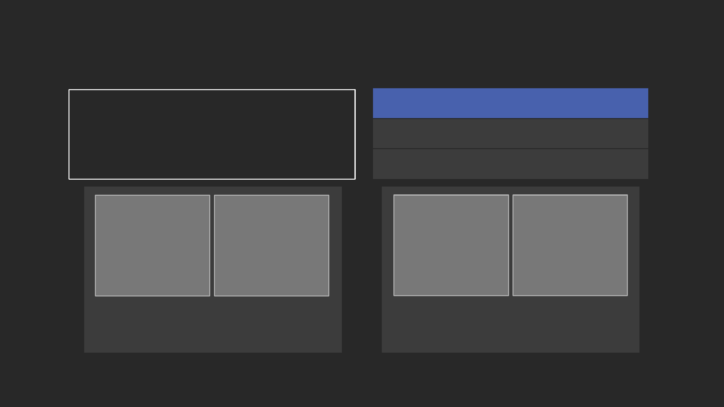
Concurrency scaling

How it works:

All queries go to the leader

node, user only sees less wait

for queries

When queries in designated

WLM queue begin queuing,

Amazon Redshift automatically

routes them to the new clusters,

enabling Concurrency Scaling

automatically

Amazon Redshift automatically

spins up a new cluster, processes

waiting queries, and

automatically shuts down the

Concurrency Scaling cluster

For every 24 hours that your

main cluster is in use, you

accrue a one-hour credit for

Concurrency Scaling. This

means that Concurrency

Scaling is free for >97%

of customers.

Amazon Redshift automatically adds transient clusters,

in seconds, to serve sudden spike in concurrent requests

with consistently fast performance

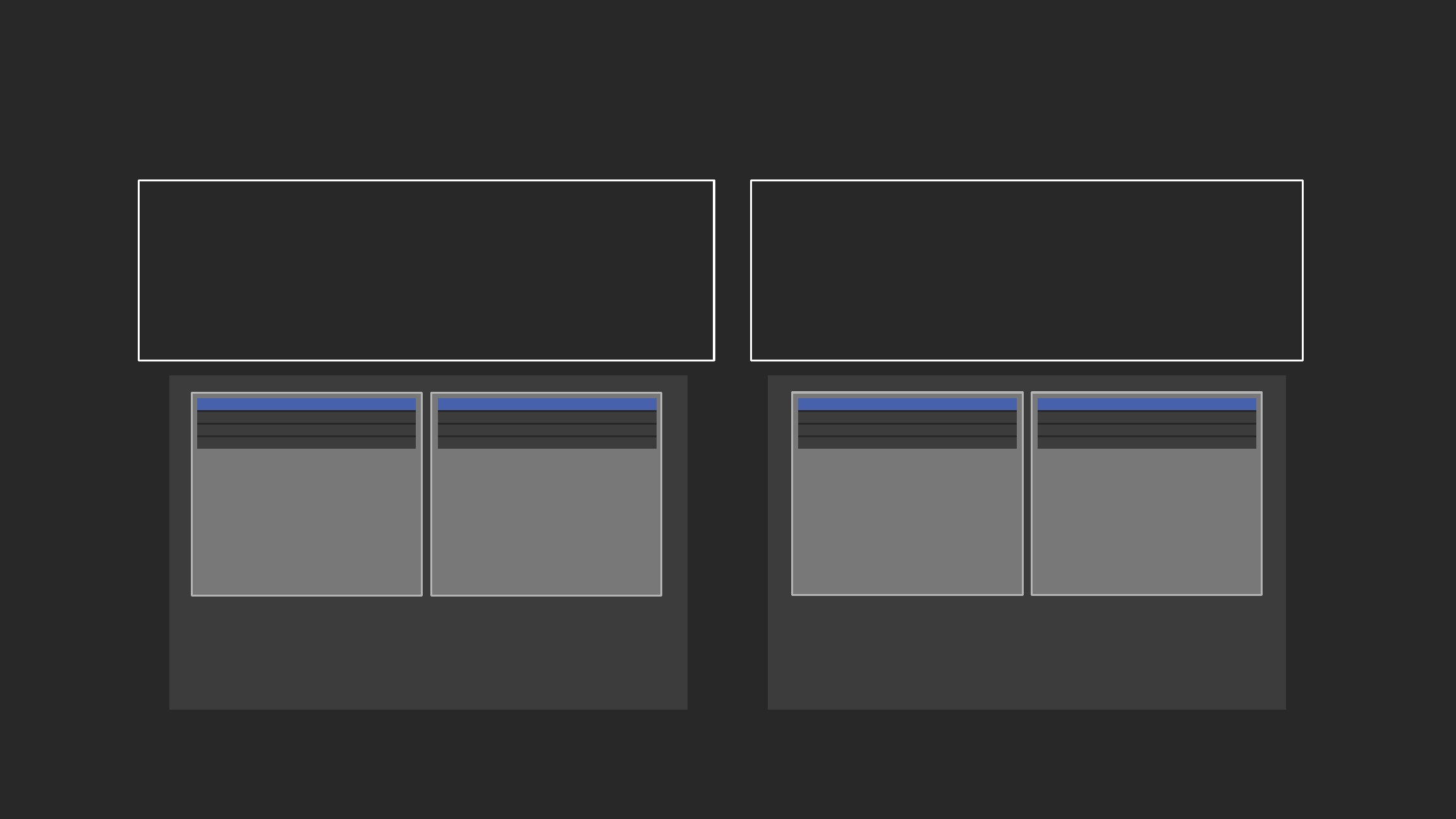
Concurrency scaling

How it works:

All queries go to the leader

node, user only sees less wait

for queries

When queries in designated

WLM queue begin queuing,

Amazon Redshift automatically

routes them to the new clusters,

enabling Concurrency Scaling

automatically

Amazon Redshift automatically

spins up a new cluster, processes

waiting queries, and

automatically shuts down the

Concurrency Scaling cluster

For every 24 hours that your

main cluster is in use, you

accrue a one-hour credit for

Concurrency Scaling. This

means that Concurrency

Scaling is free for >97%

of customers.

Amazon Redshift automatically adds transient clusters,

in seconds, to serve sudden spike in concurrent requests

with consistently fast performance

Backup

Concurrency scaling

How it works:

All queries go to the leader

node, user only sees less wait

for queries

When queries in designated

WLM queue begin queuing,

Amazon Redshift automatically

routes them to the new clusters,

enabling Concurrency Scaling

automatically

Amazon Redshift automatically

spins up a new cluster, processes

waiting queries, and

automatically shuts down the

Concurrency Scaling cluster

For every 24 hours that your

main cluster is in use, you

accrue a one-hour credit for

Concurrency Scaling. This

means that Concurrency

Scaling is free for >97%

of customers.

Amazon Redshift automatically adds transient clusters,

in seconds, to serve sudden spike in concurrent requests

with consistently fast performance

Backup

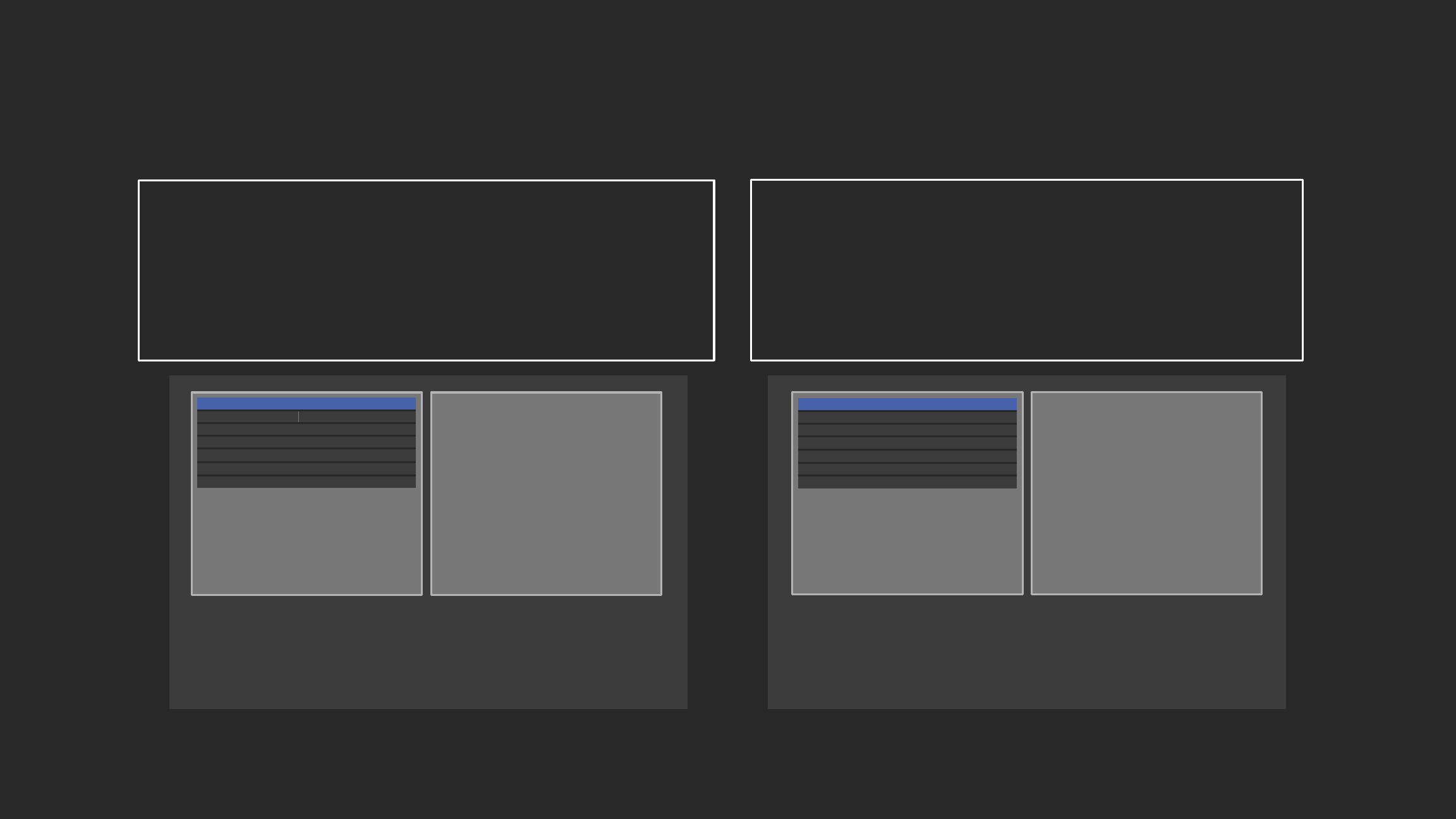
Caching Layer

Concurrency scaling

How it works:

All queries go to the leader

node, user only sees less wait

for queries

When queries in designated

WLM queue begin queuing,

Amazon Redshift automatically

routes them to the new clusters,

enabling Concurrency Scaling

automatically

Amazon Redshift automatically

spins up a new cluster, processes

waiting queries, and

automatically shuts down the

Concurrency Scaling cluster

For every 24 hours that your

main cluster is in use, you

accrue a one-hour credit for

Concurrency Scaling. This

means that Concurrency

Scaling is free for >97%

of customers.

Amazon Redshift automatically adds transient clusters,

in seconds, to serve sudden spike in concurrent requests

with consistently fast performance

Backup

Caching Layer

How it works:

All queries go to the leader

node, user only sees less wait

for queries

When queries in designated

WLM queue begin queuing,

Amazon Redshift automatically

routes them to the new clusters,

enabling Concurrency Scaling

automatically

Amazon Redshift automatically

spins up a new cluster, processes

waiting queries, and

automatically shuts down the

Concurrency Scaling cluster

For every 24 hours that your

main cluster is in use, you

accrue a one-hour credit for

Concurrency Scaling. This

means that Concurrency

Scaling is free for >97%

of customers.

Concurrency scaling

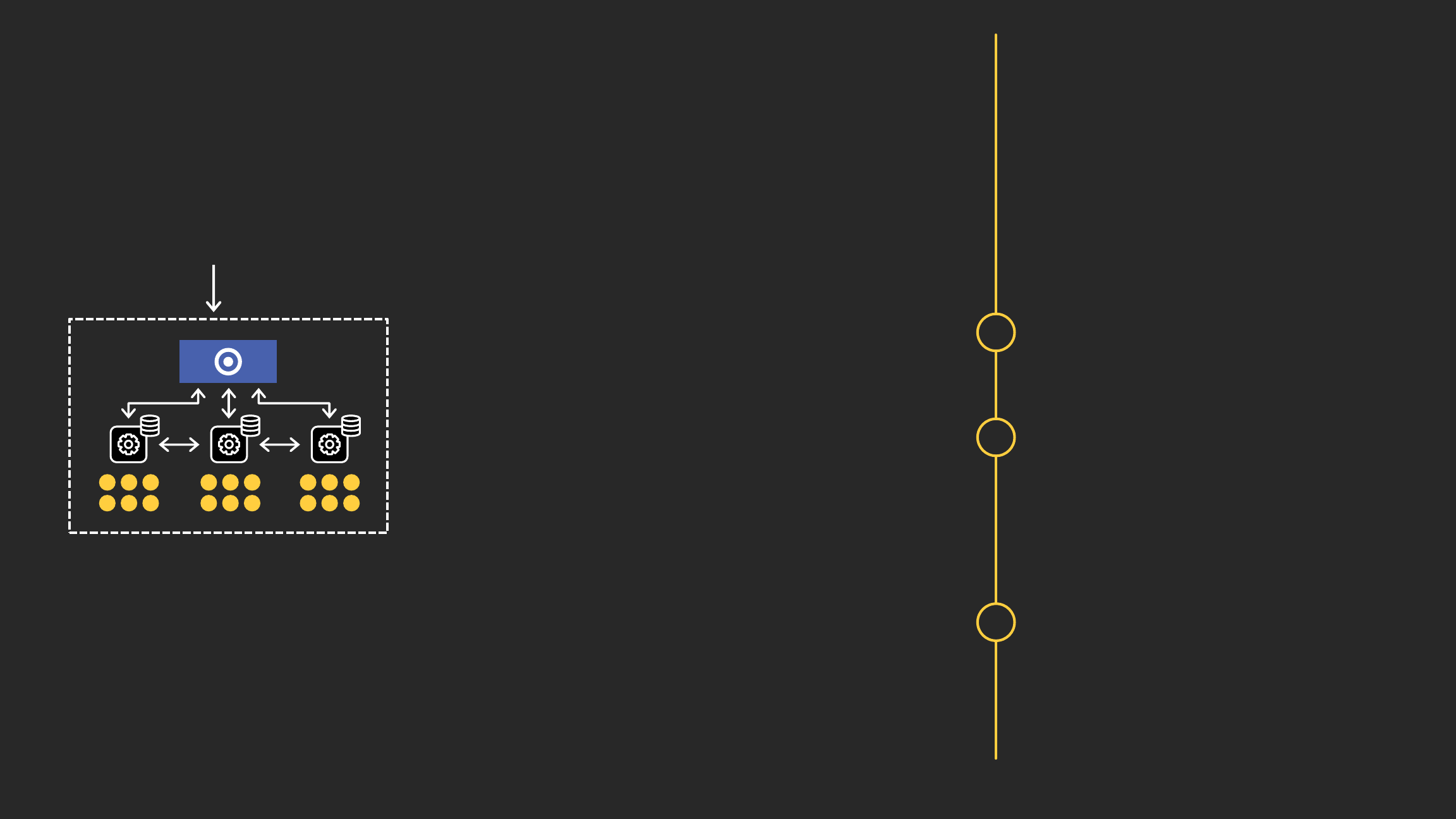
Workload management: Example

Use case:

Light ingestion/ELT on a continuous cadence of 10 minutes

Peak reporting workload during business hours (7 am–7 pm)

Heavy ingestion/ELT nightly (11 pm–3 am)

User types:

Business reporting and dashboards

Analysts and data science teams

Database administrators

Workload management: Example manual WLM

• Enable: Short Query Acceleration

• Hidden superuser queue can be

used by admins, manually switched

into:

SET query_group TO

'superuser'

• The superuser queue has a single

slot, the equivalent of 5–7%

memory allocation, and no timeout

Create a queue for each workload type:

Terminology and concept: Dynamic WLM

Manual WLM dynamic attributes

Percent of memory

Concurrency/queue slots

Concurrency scaling

Query timeout

Enable short query acceleration

Changes to dynamic properties does not require a restart, it’s a simple API call

Dynamic Workload Management Utility

https://github.com/awslabs/amazon-redshift-utils/tree/master/src/WorkloadManagementScheduler

WLM: Example (11 pm–3 am)

Enable: Short Query Acceleration

Increase memory and concurrency

for ingestion queue

Decrease memory and concurrency

for dashboard and default queues

Automatic workload management (Auto WLM)

Allows for prioritization of different query workload

Goals

Simplify WLM

Automatically controls concurrent number of executing queries

Automatically divides cluster memory

Auto WLM: Example

Automatically manages memory allocation and concurrency of queries

Query monitoring rules (QMR)

Extension of workload management (WLM)

Allow the automatic handling of runaway (poorly written) queries

Rules applied to a WLM queue allow queries to be:

LOGGED

ABORTED

HOPPED

Goals

Protect against wasteful use of the cluster

Log resource-intensive queries

Query monitoring rules (QMR)

Metrics with operators and values (e.g., return_row_count > 10000000)

create a predicate

Multiple predicates can be AND-ed together to create a rule

Multiple rules can be defined for a queue in WLM. These rules are OR-ed together

If { rule } then [action]

{ rule : metric operator value } e.g.: rows_scanned > 1000000

Metric: cpu_time, query_blocks_read, rows scanned, query execution time, cpu &

io skew per slice, join_row_count, etc.

Operator: <, >, ==

Value: integer

[action]: hop, log, abort

Best practices: WLM and QMR

Use Auto WLM—if you aren’t sure how

to set up WLM or your workload is

highly unpredictable, or you are using

the old default WLM

Use manual WLM—if you understand

your workload patterns or require

throttling certain types of queries

depending on the time of day

Keep the number of WLM queues to a

minimum, typically just three queues

to avoid having unused queues

https://github.com/awslabs/amazon-redshift-

utils/blob/master/src/AdminScripts/

wlm_apex_hourly.sql

Use WLM to limit ingestion/ELT

concurrency to two to three

To maximize query throughput, use

WLM to throttle the number of

concurrent queries to 15 or less

Use QMR rather than WLM to set

query timeouts

Use QMR to log long-running queries

Save the superuser queue for

administration tasks and

canceling queries

Cluster sizing and resizing

Sizing Amazon Redshift cluster for production

Estimate the uncompressed size of the incoming data

Assume 3x compression (actual can be >4x)

Target 30–40% free space (resize to add/remove storage as needed)

Disk utilization should be at least 15% and less than 80%

Based on performance requirements, pick SSD or HDD

If required, additional nodes can be added for increased performance

Example: 20 TB of uncompressed data ≈ 6.67 TB compressed

Depending on performance requirements, recommendation:

2-6xRA3.4xlarge or 4xDC2.8xlarge or 5xDS2.xlarge ≈10TB of capacity

Resizing Amazon Redshift

Classic resize

Data is transferred from old cluster to new cluster (within hours)

Change node types

Elastic resize

Nodes are added/removed to/from existing cluster (within minutes)

Node 1

SQL Clients/BI Tools

Leader

node

JDBC/ODBC

Node 2

Node 3

Binary data transfer

• Source cluster is placed into read-only mode during resize

• All data is copied and redistributed on the target cluster

• Allows for changing node types

Classic resize

48-slice cluster

DC2.8XL

Instances

Read-Only

Leader

node

Node 1 Node 2 Node 3 Node 4

Redirect DNS/bounce connections

Elastic resize

Node 1

SQL Clients/BI Tools

Leader

Node

JDBC/ODBC

Node 2

Node 3

Amazon S3

Node 4

Elastic

resize is

requested

15 ±10 min

Elastic

resize

starts

Elastic

resize

finishes

~4 min

Backup

• At the start of elastic resize, we take

an automatic snapshot to Amazon

S3 and provision the new node(s)

• Cluster is fully available for reads

and writes

Data transfer

finishes

Node rehydrated from Amazon S3

Restore

• Slices are redistributed to/

from nodes

• Inflight queries/connections are put

on hold

• Some queries within transactions

maybe rollback

• Cluster is fully available; data

transfer continues in the background

• Hot blocks are moved first

Elastic resize node increments

Instance type Allowed increments

Max change from

original size

Example: valid sizes

for 4-node cluster

RA3 4xlarge

DC2 large

DS2 xlarge

2x or ½ original cluster

size only

Double, ½ size 2, 4, 8

RA3 16xlarge

DC2 8xlarge

DS2 8xlarge

Can allow ± single

node increments so

long as slices remain

balanced

Double, ½ size 2, 3, 4, 5, 6, 7, 8

Elastic resize Classic resize

Scale up and down for workload spikes

✔

Incrementally add/remove storage

✔

Change cluster instance type (SSD ←→ HDD)

✔

If elastic resize is not an option because of

sizing limits

✔

Limited availability during resize

<5 minutes

(parked connections)

1–24 hours

(read-only)

When to use elastic vs. classic resize

Best practices: Cluster sizing

Use at least two computes nodes

(multi-node cluster) in production for

data mirroring

• Leader node is given for no additional cost

Maintain at least 20% free space or

three times the size of the largest table

• Scratch space for usage, rewriting tables

• Free space is required for vacuum to re-sort table

• Temporary tables used for intermediate query results

The maximum number of available

Amazon Redshift Spectrum nodes is a

function of the number of slices in the

Amazon Redshift cluster

If you’re using DS2 instances,

migrate to RA3

If you’re using DC1 instances, upgrade

to the DC2 instance type

• Same price as DC1, significantly faster

• Reserved Instances can be migrated without

additional cost in the AWS Console

Amazon Redshift Advisor

Amazon Redshift Advisor available in Amazon Redshift Console

Runs daily scanning operational metadata

Observes with the lens of best practices

Provides tailored high-impact recommendations to optimize

your Amazon Redshift cluster for performance and cost savings

Amazon Redshift Advisor: Recommendations

Recommendations include

• Skip compression analysis during COPY

• Split Amazon S3 objects loaded by COPY

• Compress Amazon S3 file objects loaded by COPY

• Compress table data

• Reallocate Workload Management (WLM) memory

• Cost savings

• Enable short query acceleration

• Alter distribution keys on tables

Additional resources

AWS Labs on GitHub: Amazon Redshift

https://github.com/awslabs/amazon-redshift-utils

https://github.com/awslabs/amazon-redshift-monitoring

https://github.com/awslabs/amazon-redshift-udfs

Admin scripts

Collection of utilities for running diagnostics on your cluster

Admin views

Collection of utilities for managing your cluster, generating schema DDL, and so on

Analyze Vacuum utility

Utility that can be scheduled to vacuum and analyze the tables within your Amazon Redshift cluster

Column Encoding utility

Utility that will apply optimal column encoding to an established schema with data already loaded

AWS big data blog: Amazon Redshift

Amazon Redshift Engineering’s Advanced Table Design Playbook

https://aws.amazon.com/blogs/big-data/amazon-redshift-engineerings-advanced-table-design-playbook-preamble-

prerequisites-and-prioritization/

—Zach Christopherson

Top 10 Performance Tuning Techniques for Amazon Redshift

https://aws.amazon.com/blogs/big-data/top-10-performance-tuning-techniques-for-amazon-redshift/

—Ian Meyers and Zach Christopherson

Twelve Best Practices for Amazon Redshift Spectrum

https://aws.amazon.com/blogs/big-data/10-best-practices-for-amazon-redshift-spectrum/

—Po Hong and Peter Dalton

Learn databases with AWS Training and Certification

Resources created by the experts at AWS to help you build and validate

database skills

25+ free digital training courses cover topics and services related

to databases, including

• Amazon Aurora

• Amazon Neptune

• Amazon DocumentDB

• Amazon DynamoDB

Validate expertise with the new AWS Certified Database—

Specialty beta exam

Visit aws.training

• Amazon ElastiCache

• Amazon Redshift

• Amazon RDS

Thank you!