Can Non-Interest Rate Policies Stabilize Housing Markets

NBER WORKING PAPER SERIES

CAN NON-INTEREST RATE POLICIES STABILIZE HOUSING MARKETS? EVIDENCE

FROM A PANEL OF 57 ECONOMIES

Kenneth N. Kuttner

Ilhyock Shim

Working Paper 19723

http://www.nber.org/papers/w19723

NATIONAL BUREAU OF ECONOMIC RESEARCH

1050 Massachusetts Avenue

Cambridge, MA 02138

December 2013

We are grateful for comments by seminar participants at the Bank for International Settlements, Williams

College, the RBA-BIS Conference on Property Markets and Financial Stability in Sydney and the

Money, Macro and Finance Conference 2013 in London. We thank Claudio Borio, Frank Packer and

Peter Pedroni for helpful suggestions and Bilyana Bogdanova, Marjorie Santos, Jimmy Shek and Agne

Subelyte for their excellent research assistance. The views presented here are solely those of the authors

and do not necessarily represent those of the Bank for International Settlements or the National Bureau

of Economic Research.

NBER working papers are circulated for discussion and comment purposes. They have not been peer-

reviewed or been subject to the review by the NBER Board of Directors that accompanies official

NBER publications.

exceed two paragraphs, may be quoted without explicit permission provided that full credit, including

Can Non-Interest Rate Policies Stabilize Housing Markets?

Evidence from a Panel of 57 Economies

Kenneth N. Kuttner and Ilhyock Shim

NBER Working Paper No. 19723

December 2013

JEL No. G21,G28,R31

ABSTRACT

Using data from 57 countries spanning more than three decades, this paper investigates the effectiveness

of nine non-interest rate policy tools, including macroprudential measures, in stabilizing house prices

and housing credit. In conventional panel regressions, housing credit growth is significantly affected

by changes in the maximum debt-service-to-income (DSTI) ratio, the maximum loan-to-value ratio,

limits on exposure to the housing sector and housing-related taxes. But only the DSTI ratio limit has

a significant effect on housing credit growth when we use mean group and panel event study methods.

Among the policies considered, a change in housing-related taxes is the only policy tool with a discernible

impact on house price appreciation.

Kenneth N. Kuttner

Department of Economics

Williams College

Schapiro Hall

24 Hopkins Hall Drive

Williamstown, MA 01267

and NBER

[email protected]

Ilhyock Shim

Bank for International Settlements

Representative Office for Asia and the Pacific

78th floor, Two IFC, Central, Hong Kong

[email protected]

1 Introduction

Following the housing boom and bust of the mid-2000s, the drawbacks of relying on interest rates

alone to ensure ﬁnancial stability have become increasingly clear. As documented elsewhere,

the quantitative impact of interest rates on house prices is economically signiﬁcant but not large

enough to achieve a meaningful degree of restraint.

An interest rate hike of sufﬁcient size to

meaningfully dampen house price growth would therefore run the risk of causing a recession.

As Federal Reserve Chairman Ben Bernanke (2010) put it, monetary policy is a “blunt tool” for

stabilizing housing markets.

Moreover, countries with exchange rate targets (either explicit or

implicit) lack the freedom to use the interest rate as a policy tool.

The recognition of interest rates’ limitations has left policymakers searching for other policy

tools to tame housing and other asset markets, either independently or as a complement to interest

rate policy. A great deal of attention has been focused on non-interest rate policies, such as reserve

requirements and maximum loan-to-value (LTV) ratios, which have been on high and growing

demand in many economies. Given the central role of the housing market in the recent crises, it

is no surprise that many of these policies are aimed squarely at reining in the housing sector. The

critical question is whether these non-interest rate tools really work in modulating house prices and

housing credit growth.

This paper is closely related to the rapidly expanding literature on macroprudential policy,

whose overarching goal is to limit systemic risk in the ﬁnancial system as a whole.

The two main

objectives of macroprudential policy are, ﬁrst, to promote the resilience of the ﬁnancial system by

mandating higher levels of liquidity, capital and collateralization; and second, to restrain the build-

up of ﬁnancial imbalances by slowing credit and asset price growth. This paper deals with the

second of these two objectives, focusing speciﬁcally on imbalances in the housing market. At the

same time, it looks at a broad range of policy actions, not just those traditionally associated with

macroprudential regulation. These include changes in taxes and subsidies affecting the housing

See Kuttner (2014) and the references contained therein.

Partly for this reason, many macroeconomists have argued that the interest rate should not be used to address such

developments (e.g. Bernanke & Gertler (1999), Blanchard et al. (2010), Gal

ı (2013), Ito (2010), Posen (2006) and

Svensson (2010)). Others have argued that there is a role for interest rate policy in ensuring ﬁnancial stability (e.g.

Borio (2011), Eichengreen et al. (2011), King (2013), Mishkin (2011), Stein (2013) and Woodford (2012)).

See IMF-BIS-Financial Stability Board (2011) for a more complete discussion of macroprudential policy.

market, and other actions, such as changes in reserve requirements, that are not explicitly justiﬁed

by macroprudential objectives. We therefore refer to the policies in our paper as credit and housing-

related tax policies, rather than as narrowly-deﬁned macroprudential tools.

A growing body of research has documented the use of tools other than the short-term interest

rate in various countries and examined their effectiveness in damping credit growth and house

prices. Among the ﬁrst was Hilbers et al. (2005), who documented that ten of the 18 central and

eastern European (CEE) countries responded to house price booms with regulatory policy actions.

In the same vein, Crowe et al. (2011) found that out of 36 countries that had experienced real

estate booms, 24 had responded with policy measures intended dampen the property market.

Focusing on six countries in Latin America, Tovar et al. (2012) showed that macroprudential

policy in general, and reserve requirements in particular, had a moderate but transitory impact on

private bank credit growth in the region. More recent work on the CEE economies by Vandenbuss-

che et al. (2012) found that certain types of macroprudential policies, including capital adequacy

ratios and non-standard liquidity measures, inﬂuenced house price inﬂation. And taking an inter-

national perspective, Borio & Shim (2007) documented 12 types of macroprudential policy actions

taken by 18 European and Asian countries going back as far as 1988. Their event study analysis

showed that macroprudential measures reduced credit growth by 4 to 6 percentage points in the

years immediately following their introduction, while house prices decelerated in real terms by 3

to 5 percentage points.

Lim et al. (2011) used data from a survey conducted by the International Monetary Fund (IMF)

in 2010 to document that 40 of the 49 countries surveyed had taken (broadly deﬁned) macropruden-

tial measures in the preceding 10 years. Using panel regression analysis, they found that a variety

of macroprudential tools, including reserve requirements, dynamic provisioning, maximum LTV

ratios, maximum debt-service-to-income (DSTI) ratios and limits on foreign currency lending had

measurable effects on the growth rate or cyclicality of private sector credit and leverage.

Taking a disaggregated approach, Claessens et al. (2013) analyzed the use of macroprudential

policy aimed at reducing vulnerabilities in individual banks in both advanced and emerging mar-

ket economies, using a sample of about 2,300 banks in 48 countries and macroprudential policy

measures documented by Lim et al. (2011). They showed that policy measures such as maximum

LTV and DSTI ratios and limits on foreign currency lending are effective in reducing leverage,

asset and non-core to core liabilities growth during booms, and that few policies help stop declines

in bank leverage and assets during downturns.

This paper’s goal is to provide a systematic assessment of the efﬁcacy of credit and housing-

related tax policies on housing credit and house prices. The analysis uses a new dataset on the

usage of nine of these policy types by 60 countries over a period going as far back as 1980, making

it the most comprehensive study to date in terms of both scope and time span. While in some

respects similar to Lim et al. (2011), our focus is on housing credit and house prices rather than

overall private sector credit. Our study employs three different empirical approaches as a check on

the results’ robustness.

The main ﬁndings are, ﬁrst, that the maximum DSTI ratio is the policy

tool that most consistently affects housing credit growth, with a typical policy tightening slowing

housing credit growth by roughly 4 to 7 percentage points over the following four quarters. Second,

the evidence suggests that an increase in housing-related taxes can slow the growth of house prices,

although this ﬁnding is somewhat sensitive to the choice of econometric method.

The plan of the paper is as follows. Section 2 describes each of the nine policies analyzed

and sketches a theoretical framework illustrating the channels through which the policies operate.

Section 3 describes the data used in the analysis, focusing on the key characteristics of the policy

action dataset. Section 4 describes the econometric methods and reports the results. Section 5

concludes.

2 The operation of credit and housing-related tax policies

The purpose of this section is, ﬁrst, to provide some speciﬁcs on how these policies operate in

practice; and second, to present bare-bones theoretical frameworks to illuminate the conditions

necessary for certain types of policies to be effective and the reasons why the effect of policies

might vary between countries.

This paper builds on Kuttner & Shim (2012), which explored a similar set of issues. The present paper uses a

signiﬁcantly expanded version of the policy action dataset used in the earlier work and brings additional econometric

methods to bear on the analysis.

2.1 General credit policies

The three policies in this category are reserve requirements, liquidity requirements and limits on

credit growth. All apply to the banking system. Because none of the three is aimed speciﬁcally

at the housing sector, we refer to them collectively as general credit policies. They might also be

characterized as non-interest rate monetary policy tools.

Reserve requirements compel banks to hold at least a fraction of their liabilities as liquid re-

serves. These are normally held either as reserve deposits at the central bank or as vault cash. The

regulation generally speciﬁes the size of required reserves according to the type of deposits (e.g.

demand, savings or time deposits), their currency of denomination (domestic or foreign currency)

and their maturity.

Liquidity requirements are typically in the form of a minimum ratio of highly liquid assets, such

as government securities and central bank paper, to certain types of liabilities. These are prudential

regulations whose main objective is to ensure a bank’s ability to withstand cash outﬂows under

stress. The main difference between liquidity and reserve requirements is that the former requires

the bank to keep funds at the central bank whereas the latter oblige them to hold liquid marketable

securities. The two policies are very similar in terms of their economic effect, as both inﬂuence

the volume of funds available for lending to the private sector by imposing constraints on the

composition of banks’ balance sheets.

Finally, limits on the expansion of private sector credit are sometimes imposed during lending

booms. This may take the form of a numerical ceiling on the rate of credit growth per month or

year, or a maximum amount of the increase in lending per month or per quarter. Another aspect of

those policies is a set of penalties on violating the speciﬁed limit.

A deposit-dependent bank

The starting point for modelling banks’ loan supply is the proﬁt-maximizing choice of balance

sheet composition. Proﬁts for a bank whose sole source of funds consists of reservable demand

deposits would be

Π = r

· L + r

· R − r

· D (1)

where L, R and D are loans, reserves and demand deposits, and r

, r

and r

are the corresponding

interest rates.

If banks hold some ﬁxed regulatory mandated share ψ of deposits as reserves, the expression

for proﬁts can be written as

Π = [r

− r

− ψ(r

− r

)

| {z }

reserve tax

]D . (2)

And since L = (1 − ψ)D, proﬁts can be also expressed as a function of L,

Π = [r

− r

− ψ(r

− r

)](1 − ψ)

−1

L . (3)

For simplicity, we assume that the reserve requirement constraint holds with equality.

If interest rates were exogenous, then the supply of loans would be perfectly elastic: for Π > 0

the bank would supply an inﬁnite amount of funds, and zero if Π < 0. The supply curve would

be a horizontal line at r

= (1 − ψ)

−1

− ψr

). An increase in ψ shifts the supply curve up, as

would a decrease in r

Equilibrium requires either that r

is an increasing function of D, or that r

is a decreasing

function of L. One way to determine the equilibrium is to have a downward-sloping loan demand

curve. In this model, households demand a greater amount of housing loans to support more con-

sumption of housing services only when the loan rate r

decreases. This can be rationalized in a

utility-maximizing model with declining marginal utility in the consumption of housing services.

Note that there is nothing “special” about banks in this model. Reserve requirements affect equi-

librium L only if one assumes that banks are the only source of ﬁnance, or that at least some subset

of households are bank-dependent.

Another way to obtain a downward-sloping loan demand curve is to assume that the agency

costs associated with lending are a function of leverage, and hence L. Increases in the interest rate

have the effect described above, but by decreasing the value of collateral, they also increase

The model omits capital for simplicity’s sake.

Banking systems differ greatly across countries in the degree to which reserve requirements are binding. As of

April 2012, the Korean banking system held virtually no excess reserves, while that of the Philippines held only 4.6

billion pesos ($100 million). Until the quantitative easing policies that began in 2008, the US banking system held only

a trivial amount of excess reserves. In contrast, the ﬁgure for Thailand is 2 trillion baht ($45 billion), the equivalent to

almost one ﬁfth of GDP.

information costs. This drives a wedge between the lending rate and the cost of funds, the essence

of the broad credit channel or “ﬁnancial accelerator.” If so, then the increase in agency costs

brought on by an increase in r

reduces lending to affected households. Of course, for this to have

an aggregate effect requires that the unconstrained households do not just step in and ﬁll the gap

in housing purchases left by the reduction in spending by the constrained households.

A third way to obtain an equilibrium is to assume that r

is an upward-sloping function of

D. One way is to relax the assumption that the reserve requirement is always binding. It would

be possible, for example, to assume a loss function that penalizes deviations from target level of

reserves. Lending reduces the desired level of reserves, which is costly. Also, attracting deposits

requires getting households to save more, which requires a higher r

To summarize, in this framework changes in reserve requirements will affect housing credit

only if:

1. Some subset of households is bank-dependent for whatever reason (by ﬂatly assuming it or

by motivating it in a model with agency costs).

2. The reduction in credit demand coming from constrained borrowers is not offset by bor-

rowing by unconstrained borrowers. This would be true if the marginal product of ﬁrms’

investment projects were declining (as in the neoclassical model) or if unconstrained bor-

rowers had a downward-sloping demand for housing (this ties into the model of household

utility maximization).

3. Some share of any change in total bank lending is manifested in changes in housing credit.

A bank with non-reservable funding sources

The banking model sketched above is unrealistic to the extent that banks rely on non-reservable

funding sources that allow them to increase lending without being constrained by reserve require-

ments. This is highly relevant to the United States, where total bank reserves fell from $30 billion

in 1994 to $10 billion in 2006, even as commercial bank credit grew from $3 trillion to $7 trillion.

The same issue would arise if lending were securitized and removed from banks’ balance sheets,

as was the bulk of housing credit in the United States during the boom.

The banking model can be made more realistic by allowing banks to raise funds through reserv-

able demand deposits, DD, and non-reservable certiﬁcates of deposit, CD. Proﬁts are now given

Π = r

· L + r

· R − r

· DD − r

·CD . (4)

Since L = (1 − ψ)DD +CD, proﬁts can be also expressed as a function of L and DD,

Π = (r

− r

)L + (r

− r

)DD − ψ(r

− r

)DD . (5)

For simplicity, assume that DD is ﬁxed and that CD is the marginal source of funding. The loan

supply curve would then be a horizontal line at r

= r

. As in the case without non-reservable

funding, one way to obtain an equilibrium in the loan market is to assume downward-sloping loan

demand curve.

Another way to obtain an equilibrium is to assume an upward-sloping supply of non-reservable

CDs, which would translate into an upward-sloping loan supply curve. This assumption also makes

it possible for reserve requirements to affect loan supply. An increase in ψ would reduce the

supply of funds coming from DD, and given L, this would require an increase in CD. If the supply

of CDs is upward-sloping (perhaps because it increases the agency costs associated with banks’

borrowing), then this would raise banks’ cost of funds and shift the loan supply curve upward.

To summarize, if banks can obtain non-reservable funding, then in addition to the three condi-

tions enumerated previously, we have to assume that

4. The supply curve for non-reservable funding is upward-sloping.

2.2 Targeted credit policies

A second category of credit policies encompasses those intended speciﬁcally to limit the growth of

housing credit. These include the imposition of a maximum LTV or DSTI ratio, both of which af-

fect households’ demand for housing credit. Supply-side tools are also used to restrain the volume

of housing credit supplied by the banking system. These include the imposition of limits on ex-

posure to the housing sector, the adjustment of risk weights applied to housing loans and changes

in provisioning requirements. Since these ﬁve types of measures are also intended to limit banks’

and households’ exposure to risk, they might also be referred to as prudential policy tools.

2.2.1 Demand-side policy instruments

In order to slow housing loan growth and build up buffers within banks against potential losses

from housing loans, national authorities often either impose a maximum LTV ratio applied to home

mortgages or lower the pre-existing maximum. The authorities may also prohibit certain types of

housing loans, which is equivalent to applying a zero LTV ratio. For example, when housing

markets were overheating in 2012, the Chinese authorities prohibited banks from making loans to

purchase second or third houses and also barred foreigners and non-residents from borrowing from

banks to purchase houses.

Another frequently used way of restricting the excessive provision of housing credit is to limit

the DSTI ratio (or debt service ratio) applied to the borrowing of home buyers. Typically, reg-

ulators specify a certain percentage of the borrower’s monthly income as the maximum monthly

repayment on a bank loan. Less frequently, limits to the loan amount can be expressed as a mul-

tiple of household income (i.e. maximum debt-to-income ratio) or regulators can limit the mini-

mum debt-repayment-to-debt ratio. Alternatively, authorities can lengthen the maximum maturity

of mortgage contracts or introduce preferential interest rates for mortgage loans, thus easing the

repayment burden for mortgage borrowers. All such measures are classiﬁed as “other lending

criteria.”

A simple two-period utility maximizing model can be used to shed light on the impact of

demand-side credit instruments. Households choose between consumption today, consumption

tomorrow, and the quantity of housing:

max

u(c

) +

1 + ρ

u(c

) + v(h) (6)

such that

+ p

h +

1 + r

≤

1 + r

+ y

1 + r

. (7)

In the context of an overlapping generations model, period 1 would represent the early part of the

life cycle in which households purchase a home (for a price p

), and period 2 represents retirement

in which households draw down housing equity in order to ﬁnance consumption (i.e. they sell the

house for a price p

The two ﬁrst-order conditions are the usual consumption Euler equation,

) =

1 + r

1 + ρ

) (8)

and

) =



r − π

1 + r



−1

(h) . (9)

The term in square brackets is the user cost of home ownership and π is the expected rate of house

price appreciation.

Alternatively, the household could pay rent R to obtain housing services in periods 1 and 2, in

which case the ﬁrst-order condition would be

) = R

−1

(h) . (10)

Equations 9 and 10 together imply that if households are unconstrained, then in equilibrium, rent

and user cost will be equal.

Combining the ﬁrst-order conditions with the budget constraint will yield a downward-sloping

demand for h as a function of π, r, p

and permanent income. Note that borrowing in the ﬁrst

period is equal to c

+ p

h − y

A limit on the DSTI ratio imposes the following condition on the budget constraint:

credit = c

+ p

h − y

≤ φy

/r . (11)

At the risk of stating the obvious, the DSTI constraint becomes less likely to bind as the interest

rate declines.

Analogously, a limit on the LTV ratio looks like:

credit = c

+ p

h − y

≤ θ p

h . (12)

Physical depreciation is ignored in order to keep things simple. Taxes, which also affect the user cost, are discussed

below.

Again noting the obvious, the existence of a maximum LTV ratio allows housing credit to rise along

with the house price or forces housing credit to fall along with the house price. This suggests that

a reduction in the maximum LTV ratio (tightening) is likely to be less effective than a reduction

in the maximum DSTI ratio (tightening) when it comes to restraining credit growth during house

price booms.

For example, suppose that the actual LTV ratio equals the maximum LTV ratio of 80%. When

the value of a house increases by 15% this year, under the current maximum LTV ratio households

can borrow 15% more. Therefore, even after the maximum LTV ratio is lowered by 10 percentage

points from 80% to 70% this year, the credit growth over the year is positive. By contrast, house-

hold income does not typically grow over a year as fast as house prices, so there is more room for

tightening the maximum DSTI ratio to be effective than for tightening the LTV ratio by the same

amount. Likewise, an increase in the maximum LTV ratio (loosening) seems to be less effective

than an increase in the maximum DSTI ratio (loosening) when it comes to promoting credit growth

during house price downturns. In particular, when the house price falls, to meet the current maxi-

mum LTV ratio the loan amount also needs to fall. Thus, an increase in the maximum LTV ratio

may not be enough to avoid a net decrease in credit. Moreover, the interaction of house prices and

housing credit over time (especially during credit-fuelled housing booms) tends to further limit the

effect of adjusting the maximum LTV ratio.

The utility function can be maximized subject to the budget constraint plus either the LTV or

the DSTI constraint (equation 11 or 12). The ﬁrst-order condition in the case of a hard borrowing

constraint case (θ = 0),

− p

h) =

(h) +

1 + π

1 + ρ

h + y

) , (13)

implicitly deﬁnes a downward-sloping demand curve for h as a function of π, r, p

and permanent

income. Note that this is very similar to the consumption Euler equation: housing earns a rate

of return π and functions as a vehicle for saving, but the v

term says that the the household also

receives utility from the house it owns.

The demand curve under the DSTI constraint is given by the analogous ﬁrst-order condition,

((1 + r

−1

φ)y

− p

h) =

(h) +

1 + π

1 + ρ

h + y

) . (14)

An increase in the binding maximum DSTI ratio, φ , means that for a given h, the household will

be able to borrow more for ﬁrst-period consumption. This reduces u

), and the household will

respond by increasing h. Note also that an increase in p

causes a one-for-one reduction in the

resources available for ﬁrst-period consumption.

The optimal allocations for different levels of the maximum DSTI ratio may be summarized as

follows:

• When the maximum DSTI ratio, φ , is not binding (the unconstrained case),

credit = p

∗

− (y

− c

∗

) ≥ 0 and debt repayment = r(c

∗

+ p

∗

− y

) < φy

. (15)

• When the maximum DSTI ratio, φ

, is binding (the constrained case),

credit = p

− (y

− c

) ≥ 0 and debt repayment = r(c

+ p

− y

) = φ

(16)

• When the maximum DSTI ratio,

φ, is binding and

φ > φ

credit = p

h − (y

− ˜c

) ≥ 0 and debt repayment = r(˜c

+ p

h − y

) =

φy

(17)

• From equations 16 and 17,

˜c

+ p

h = (1 +

φ/r)y

and c

+ p

= (1 + φ

/r)y

. (18)

Since (1 +

φ/r)y

> (1 + φ

/r)y

, ˜c

+ p

h > c

+ p

. Therefore, if ˜c

= c

h > h

and

h = h

, ˜c

> c

. This means that when the DSTI constraint is binding and the authori-

ties lower the maximum DSTI ratio, households respond either by lowering their housing

demand or by lowering their ﬁrst-period consumption.

With a binding maximum LTV requirement with 0 < θ < 1, housing demand is given by

(1 − θ)u

− (1 − θ)p

h) =

(h) +

1 + π

1 + ρ

h + y

) . (19)

A key difference between this and the DSTI-constrained demand relationship is the 1 − θ factor

multiplying u

) on the left-hand side of the equation. The factor reﬂects the fact that when

the maximum LTV ratio is binding, because a fraction of the cost of purchase is borrowed, a

one-unit increase in h causes a less than one-for-one reduction in the resources available for ﬁrst-

period consumption. An increase in the binding maximum LTV ratio, θ (loosening the constraint),

therefore, has both an inframarginal effect (increasing c

for a given h) and a marginal effect

(raising the marginal opportunity cost in terms of c

) of an increase in h. But unlike in the case of

the DSTI constraint, an increase in p

has a less than one-for-one effect on the feasible c

The optimal allocations for different levels of the maximum LTV ratio may be summarized as

follows:

• When the maximum LTV ratio, θ, is not binding (the unconstrained case),

credit = p

∗

− (y

− c

∗

) ≥ 0 and (c

∗

+ p

∗

− y

) < θ p

∗

.. (20)

• When the maximum LTV ratio, θ

, is binding (the constrained case),

credit = p

− (y

− c

) ≥ 0 and (c

+ p

− y

) = θ p

(21)

• When the maximum LTV ratio,

θ, is binding and

θ > θ

credit = p

h − (y

− ˜c

) ≥ 0 and ( ˜c

+ p

h − y

) =

θ p

h (22)

• From equations 21 and 22,

− ˜c

) = (1 −

θ)p

and

− c

) = (1 − θ

. (23)

Since (1 − θ

> (1 −

θ)p

, 1/h

− c

) > 1/

h(y

− ˜c

). Therefore, if ˜c

= c

, then

h > h

and if

h = h

, then ˜c

> c

. This means that when the LTV constraint is binding and

the authorities lowers the maximum LTV ratio, the households respond either by lowering

their housing demand or by lowering their ﬁrst-period consumption.

This is little more than a sketch of the demand for housing credit. It nonetheless sufﬁces to

highlight the ways in which the imposition of maximum LTV and DSTI ratios will affect credit

demand. Both shift the demand curve inward, although there are subtle differences having to do

with the ways in which house price appreciation and the interest rate affect the respective con-

straints. The overall effect on housing demand will, of course, depend on the share of households

that are liquidity-constrained. Deriving the implications for house prices would require the supply

side of the model to be ﬂeshed out, but clearly the impact will depend not only on the share of

credit-constrained households, but also on the slope of unconstrained households’ demand curve

for housing. If demand is highly elastic, then a drop in constrained households’ demand for hous-

ing (credit) will be offset by an increase in the housing consumed by unconstrained households.

Importantly, the existence of credit-constrained households is not a necessary condition for taxes

to affect the house price, as these directly affect the user cost of home ownership.

2.2.2 Supply-side policy instruments

The three policy tools aimed at housing credit supply are provisioning requirements, risk-weighting,

and exposure limits. The ﬁrst two are similar to reserve and liquidity requirements in the sense that

they affect bank loan supply through the cost of funds. The difference is that they apply speciﬁ-

cally to housing credit, and consequently we classify them as targeted credit policies. By contrast,

exposure limits affect the housing credit supply, not through the cost of funds but through the

quantitative limit on banks’ supply of housing loans.

By limiting the exposure of banks toward the housing or property sector as a percentage of the

total assets or liabilities, this type of measure aims to slow down rapid expansion of housing loans

by banks (and also limit the losses from housing loans when the housing prices correct and housing

loan defaults surge). A limit on housing loan exposure is sometimes set as a certain percentage of

a bank’s equity.

Under Basels I, II or III, housing loans are subject to different risk weights than corporate or

sovereign exposures. Raising risk weights on housing loans makes it more costly for banks to

extend housing loans given a ﬁxed amount of bank equity. Often, risk weights are differentiated

by the actual LTV ratio of individual loans. For example, the parts of a housing loan’s LTV ratio

that are higher than a certain threshold (say, 80%) may carry a higher risk weight. Similar to risk

weights, increases (or reductions) in general loan loss provisions and speciﬁc loan loss provisions

applied to housing loans can be used to make housing loans more (or less) costly and thus help

slow (or spur) growth in housing credit.

2.3 Housing-related tax policies

The ﬁnal category of policies considered consists of measures that affect the cost of purchasing a

home. They include taxes (such as capital gains, wealth and value added taxes), subsidies (on ﬁrst-

time home buyers and young couples and also on mortgage interest payment), fees (such as stamp

duties and registration fees) and tax deductibility of mortgage interest payments. For brevity, all

are referred to as housing-related taxes.

The effects of these taxes are easy to understand in the context of the user cost (UC) framework.

Note that the effects on the house price does not depend on the existence of credit-constrained

households. A tax increase would increase the UC even if everyone could be unconstrained. The

effects on credit depend on the elasticity of housing demand. If demand were perfectly inelastic,

the quantity of housing purchased would remain unchanged, as would housing credit.

3 Data

The analysis in Section 4 spans the period from 1980Q1 to 2011Q4 and covers 57 advanced and

emerging market economies.

These include 13 economies from the Asia-Paciﬁc region (Australia,

China, Hong Kong SAR, India, Indonesia, Japan, Korea, Malaysia, New Zealand, the Philippines,

Singapore, Thailand and Chinese Taipei), 15 from central and eastern Europe (Bulgaria, Croatia,

the Czech Republic, Estonia, Hungary, Latvia, Lithuania, Poland, Romania, Russia, Serbia, Slo-

vakia, Slovenia, Turkey and Ukraine), six from Latin America (Argentina, Brazil, Chile, Colombia,

Mexico and Peru), two from the Middle East and Africa (Israel and South Africa), two from North

America (Canada and the United States) and 19 from western Europe (Austria, Belgium, Denmark,

Finland, France, Germany, Greece, Iceland, Ireland, Italy, Luxembourg, Malta, the Netherlands,

Norway, Portugal, Spain, Sweden, Switzerland and the United Kingdom). This section summa-

rizes the data sources and the criteria used for selecting the economies and subsamples, and reports

descriptive statistics for the key variables used in the analysis.

As discussed in Section 3.3, data limitations require the United Arab Emirates, Saudi Arabia and Uruguay to be

excluded from the analysis.

3.1 The policy action dataset

The heart of the empirical analysis and a major contribution of the paper is a new, comprehen-

sive dataset of non-interest rate policies affecting housing credit and house prices. The dataset

includes 60 economies, spanning a period going back to January 1980 for some economies and

running through June 2012. The database is a superset of the one described in Shim et al. (2013),

which covers a shorter period (starting in 1990) and excludes changes in housing-related tax policy.

Appendix Table 1 provides details on the dates of coverage of the policy database.

The policy action dataset draws on a variety of sources. Wherever possible, we use ofﬁcial

documents from central banks, regulatory authorities and ministries of ﬁnance of 60 economies,

including their annual reports, ﬁnancial stability reports, monetary policy bulletins, supervisory

authorities’ circulars, budget reports, ministry of ﬁnance announcements on tax changes and press

releases from these institutions. We also consulted Borio & Shim (2007), a survey by the Com-

mittee on the Global Financial System (CGFS) on macroprudential policy conducted in December

2009, Hilbers et al. (2005), Crowe et al. (2011), Lim et al. (2011), and Tovar et al. (2012). Where

these secondary sources were used, we cross-checked the information from the secondary sources

against the information obtained from ofﬁcial documents. We then used our database of policy

actions to generate variables capturing the tightening and loosening of the policy instruments.

There are clear pros and cons to this approach. One beneﬁt is that the dataset should in princi-

ple provide a complete list of all relevant policy actions ofﬁcially published by central banks and

ﬁnancial authorities, while an ad hoc survey could suffer from incomplete identiﬁcation of relevant

policy actions. Moreover, by reading through ofﬁcial publications, we can obtain full and accurate

information on each of the potentially relevant policy actions. These details allow us to use uni-

form criteria when determining which measures to include and how to record them consistently.

Another beneﬁt of relying on ofﬁcial publications is accurate identiﬁcation of the implementation

date of each policy action. One disadvantage of using ofﬁcial sources is the language barrier for

some countries, given that English translations for such documents may be unavailable for earlier

periods. Also, for a limited number of countries, archives available on the websites of relevant au-

The IMF survey described in Lim et al. (2011) includes only those actions taken for explicitly macroprudential

purposes, and therefore excludes a large number of policy changes that are likely to have affected the housing market.

thorities or ofﬂine publication archives available from the BIS library may have one or two missing

years. Therefore, we may have omitted relevant policy actions taken in these missing years.

The policy changes are categorized along the lines laid out in Section 2. The ﬁrst category en-

compasses general credit policy measures: minimum reserve requirements, liquidity requirements

and limits on credit growth. The latter two policy actions are relatively infrequent, however, and so

in the empirical work performed below, the three are aggregated into a single variable representing

this class of policy.

The database includes changes in various forms of reserve requirements. In particular, we con-

sider changes in the reserve requirement ratio and reserve base. We do not consider changes in the

remuneration rates, reserve maintenance periods or averaging methods because we focus on policy

actions directly targeting the aggregate quantity of funds available for lending. However, it should

be noted that this distinction is not clear-cut to the extent that reserve requirements also operate,

in effect, by inﬂuencing the cost of lending. We also include both average reserve requirements,

where a certain reserve requirement ratio applies to all outstanding amount of eligible liabilities,

and marginal reserve requirements, with which additional liabilities banks assume after certain

dates or the amount of liabilities exceeding the level of banks’ liabilities as of certain dates are

subject to often very high reserve requirement ratios.

The second category consists of the targeted credit policy measures: maximum LTV ratios,

maximum DSTI ratios, risk weights on housing loans, provisioning requirements (general loan-

loss provisioning ratios and speciﬁc provisioning ratios applied to housing loans) and exposure

limits on banks to the housing sector. Finally, the third category includes housing-related tax pol-

icy measures: taxes (such as capital gains tax, wealth tax and value added tax related to housing),

subsidies (on ﬁrst-time home buyers and young couples and also on mortgage interest payment),

fees (such as stamp duties and registration fees) and tax deductibility of mortgage interest pay-

ments. We only include in the database only nationwide measures targeting middle-income or

high-income groups who are potential homebuyers. Thus, tax measures applied to one or two

cities or subsidies given speciﬁcally to low-income families are not included.

Heterogeneity is intrinsic to the policy action dataset. Even with the application of uniform

selection criteria across countries, the speciﬁcs of policy actions differ across countries and over

time. For example, the dataset includes the introduction of a maximum LTV ratio as well as the

subsequent reductions and increases in the ratio. Also, in some economies total household income

is used in calculating the DSTI, while in others the borrower’s income is used. Including these

data in a regression model therefore requires some degree of standardization and aggregation. Our

solution is to create monthly variables that take on three discrete values: 1 for tightening actions,

−1 for loosening actions and 0 for no change.

The monthly observations are summed to create

quarterly time series. This means that if multiple actions in the same direction were taken within

a given quarter, the variable could take on the values of 2 or −2, or even 3 and −3. It also means

that a tightening action and a loosening action taken within the same quarter would cancel each

other out. Changes in reserve requirements account for nearly all closely spaced actions. With

only a few exceptions, no more than one of the other types of policy actions is observed in any

given quarter.

Table 1 tabulates the different types of policy actions, aggregated by region. The dataset

contains a total of 1,111 policy actions in all, of which roughly 55% (607) are tightening, and

45% (504) are loosening. The table shows that the most active users of credit policies are the

Asia-Paciﬁc and CEE economies in terms of both the absolute number of actions recorded in the

database and the average number of actions per region per decade. The Asia-Paciﬁc economies

and western European countries are the most frequent users of housing-related tax measures. It

is also clear that reserve requirements are by far the most frequently used of the nine categories

of policy, accounting for roughly half of all the actions. Liquidity requirements and credit growth

restrictions are relatively less frequently used. Among the targeted credit policies, LTV restrictions

are most popular, followed by risk weights, DSTI restrictions, provisioning and exposure limits.

Figure 1 shows that the use of these policies varies a great deal between countries. A large share

of the countries in the sample used credit and housing-related policies only occasionally. Several

countries were very active users of these policies, with 20 or more documented policy actions per

decade. About 30% of the total number of policy changes in the dataset were taken by these very

active users.

Since the dataset documents policy actions implemented by each economy every month from

Some of the policy measures that are more standard across countries, such as reserve requirements, would be

more amenable to a numerical representation.

January 1980, we can show which types of measures were actively used over the past three decades

or so. Figure 2 shows how often each of the nine types of policy action was used over the period

from 1980 to 2012. We ﬁnd that the total number of policy actions has increased steadily from the

1980s, to 1990s, 2000s and between January 2010 and June 2012. This is also the case for the total

number of policy actions per country per decade.

The mix of policies has also varied over time. In the 1980s, more than 90% of policy actions

documented in the dataset were general credit policy measures, dominated by changes in reserve

requirements. In the 1990s, the share of general credit policy actions fell to 76%, while the share

of targeted credit policy measures increased from zero to 13%. The share of targeted credit policy

measures continued to rise in the 2000s, when it more than doubled to 28%, while that of general

credit policy measures decreased to 57%. Finally, over the two and a half years between January

2010 and June 2012, the share of general credit policy actions further declined to 51%, and at the

same time that of targeted credit policy measures increased by the same amount to 33% led by

the active use of LTV measures. It should be noted that, in contrast to the shares of general and

targeted credit policy measures that have changed substantially over the three decades or so, the

share of housing-related tax measures has remained stable between 10% and 15% over the same

period.

Table 2 shows the correlations between the various policy measures. Panel A displays the cor-

relation matrix for the discrete policy change variables. Most of these correlations are relatively

small, indicating that there is little tendency for a country to take different kinds of policy action

within the quarter. The one exception is the 0.37 correlation between DSTI and LTV actions,

suggesting that the two policies are often used in conjunction. Panel B displays the correlations

between cumulative policy indicators, constructed by summing current and previous quarters’ pol-

icy changes. This takes into account the possibility of co-movements between the policies that

may not occur within the same quarter. The relationship between the DSTI and LTV variables is

even stronger in this case, with a correlation of 0.58. There is also some evidence that changes in

provisioning requirements accompany changes in the DSTI and LTV requirements.

To give a sense of how these policies have been implemented in practice, Figures 3 to 5 dis-

See Shim et al. (2013) for more a more detailed description of policy usage.

play selected cumulative policy indicators along with the short-term nominal interest rate for three

Asian economies that have been active users of the policies. The ﬁgures show that the deployment

of these policies varies greatly from country to country. They have been used to complement con-

ventional interest rate policy in some episodes, while in others they have functioned as substitutes.

Similarly, the various credit and housing-related tax policy measures have sometimes been used in

concert, and independently at other times.

In China (Figure 3), for example, the short-term interest rate, reserve requirements, LTV and

DSTI requirements have all tended to move in the same direction: tightening in 2006–08, loosening

in 2008–09, and tightening from 2010. The relationship between the LTV and DSTI measures is

particularly close. Since 2002, there has been a steady trend towards more restrictive policy in all

three non-interest rate dimensions.

In Hong Kong SAR (Figure 4), the tightening of credit growth limits was the only monetary

tool used in 1993. Targeted credit measures (mostly changes in the maximum LTV ratio) were

used actively from the mid-1990s, usually in parallel with the general direction of interest rates in

Hong Kong SAR (as well as those in the United States). The opposite has been true since 2009,

when the LTV requirements have been progressively tightened even as the short-term interest rate

has fallen (tracking the US rate). Hong Kong authorities have also made more active use of tax

measures since 2009.

In Korea (Figure 5), reserve requirements were the primary non-interest rate policy tool used

throughout the 1990s, rising along with the short-term interest rate (except during the Asian ﬁnan-

cial crisis). Since 2002, the short-term interest rate has remained stable, but the maximum DSTI

and LTV ratios have been tightened considerably. Both ratios followed a similar upward trajectory,

although the tightening in the LTV requirements started roughly three years prior to the tightening

of the DSTI requirements. As in China, the LTV and DSTI requirements are both signiﬁcantly

more restrictive now than they were 10 years ago.

3.2 Housing credit, house price and macroeconomic data

Another contribution of the paper is its use of an extensive new dataset of house prices. The starting

point is the BIS property price database.

We enlarged this dataset using data from statistics from

Available at http://www.bis.org/statistics/pp.htm.

ofﬁcial sources and, in a few instances, from proprietary private sector sources such as CEIC.

When multiple housing price indices are available for a given economy, for example nationwide

versus major city indices, we use indices for major cities, as these are the areas that would be most

susceptible to overvaluation and are often addressed by targeted credit policy and housing-related

tax policy. Data are available for 57 economies, although the time series are quite short in many

cases. Brazil’s data only go back to 2010Q4, for example. Appendix Table 2 lists the starting and

ending dates for the house price series.

The property price data are highly imperfect. The deﬁnition of housing price indices varies

across the economies. The methods used in the construction of the price indices (e.g. quality ad-

justment) vary greatly between economies, as does the deﬁnition of the relevant housing market

(e.g. ﬂats versus detached houses). Moreover, in some cases two or more series must be spliced

together in order to yield a usable time series. In India, for example, we combined the Mumbai

housing price series provided by the Reserve Bank of India, which ends in 2010Q2, with a new

price index from the National Housing Bank, which is available from 2010Q3. Conclusions involv-

ing the level of property prices are therefore problematic, especially cross-country comparisons.

Recognizing these limitations, we will proceed on the assumption that these series can serve as

informative indicators of cyclical swings in the residential property market, if not the price levels.

Household credit data were compiled from a similarly diverse set of sources. The primary

source is the BIS data bank, supplemented with series from Datastream, CEIC and central bank

websites. Data are available for 57 countries, although for several economies the series only begin

in the late 2000s. And as with the price data, the sources and deﬁnitions are not always consistent,

even within a country. The starting and ending dates for the housing credit series are also listed in

Appendix Table 2.

The empirical work also uses a number of macroeconomic time series. One is the consumer

price index, obtained from the IMF’s International Financial Statistics database. The IMF is also

the source for most of the short-term interest rate series, supplemented in several cases with data

from national sources or Haver Analytics.

Ideally, our analysis would also include a measure of personal disposable income. These data

are difﬁcult or impossible to obtain for the majority of countries we are looking at, however. We

therefore used as a proxy annual real per capita gross national income (GNI) from World Bank’s

World Development Indicators database, interpolated to a quarterly frequency.

3.3 Sample selection criteria

Data availability is the main constraint on the scope of our analysis. As previously noted, the

United Arab Emirates lacks interest rate data while Uruguay and Saudi Arabia have no house price

or housing credit data, narrowing our sample to 57 economies. For most countries, the 2011Q4

endpoint is constrained by the GNI data, which were only available through that date at the time

of writing.

For some countries, data are available, but the time series are too short to be of any use.

Economies with fewer than 16 usable quarterly observations (accounting for the loss of obser-

vations from lags and differencing) are excluded. This criterion eliminates Brazil from the house

price regression. Similarly, Iceland and Serbia are dropped from the regressions involving housing

credit.

Even where data are available, there are often good reasons to discard a portion of the sample.

We exclude periods of extreme macroeconomic instability, as these are accompanied by extremely

high inﬂation and interest rates. Argentina’s 1990 and 2002 crises are prime examples of such

episodes. In order to prevent these anomalous observations from unduly inﬂuencing the results,

we postpone the regression start dates to avoid these periods.

Poor data quality is another reason for truncating the sample. While there is no good way to

independently verify the reliability of the data, many of the series exhibit extreme volatility during

the ﬁrst few quarters for which they are available. Some of the observed spikes may be the result

of very rapid growth from a small base, or an artifact of small samples or thin markets. This is a

common issue among the CEE economies. The regression starting date is delayed in these cases

in order to exclude these periods. Large changes that appear to genuinely reﬂect conditions in the

housing market are not dropped.

Table 3 reports descriptive statistics for the housing credit, house price and macroeconomic

data, after the sample selection criteria are applied. Even with the elimination of the most extreme

observations, there is still a great deal of volatility in the data, especially in house prices and

housing credit. The standard deviations of the annualized quarterly percentage changes in these

two variables are 15.6 and 12.3 respectively. The sample even contains changes in these two

variables in excess of 100%.

4 Empirical methods and results

This section presents estimates of the policies’ effects on housing credit and house prices. We

use three different empirical methods in an effort to assess the robustness of our results. The ﬁrst

involves conventional panel data regressions. The second uses a mean group estimator, which

allows for cross-country heterogeneity in the model coefﬁcients. The third can be described as a

panel event study analysis in which the results of country-speciﬁc event studies are aggregated to

estimate the average effect for the sample. We also explore the possibility of asymmetric responses

to policy tightenings and loosenings.

The three methods yield similar point estimates for the policies’ effects. The degree of preci-

sion varies, however, with the panel regressions producing smaller standard errors than the other

two methods. To preview, we ﬁnd that DSTI limits exert a signiﬁcant effect on housing credit

growth, a result that holds regardless of the method used. With the exception of housing-related

tax changes, none of the policies consistently affects house price growth.

4.1 Conventional panel regression analysis

We begin with a standard reduced-form regression model of credit growth,

∆ lnC

i,t

= α

+ ρ∆lnC

i,t−1

+ β

i,t−1

+ β

i,t−2

+ β

∆y

i,t−1

+ β

∆y

i,t−2

∑

j=1

i,t− j

+ ε

i,t

(24)

in which the quarterly credit growth rate for country i, ∆ lnC

, is expressed as a function of its own

lag, two lags of the short-term interest rate, r

, two lags of real personal income growth, ∆ lny

, and

a variable X

representing one (or more) of the policy variables described in Section 3. To account

for cross-country differences in the average rate of credit growth, a country-speciﬁc ﬁxed effect,

is included.

An analogous speciﬁcation is used for the house price, P

Strictly speaking, the inclusion of the lagged dependent variable would bias the ﬁxed-effect estimator. But given

the relatively long time series dimension of the data, the amount of bias should be small.

Theoretically, the user cost model implies a cointegrating relationship between house prices and rents, which

would suggest including the log of the rent-to-price ratio as an additional regressor. Results not presented in this paper

indicate that the inclusion of this term has no signiﬁcant effect on the parameter estimates of interest.

Reduced-form regressions such as equation 24 are always susceptible to the critique that the

regressors are likely to be endogenous. Speciﬁcally, policymakers may adjust interest rates or im-

plement credit and housing-related tax policies in response to conditions in the housing market (or

in response to omitted variables that are correlated with house prices or credit ﬂuctuations). This

is especially true in those economies, such as many in the Asia-Paciﬁc region, where policymakers

have actively changed LTV, provisioning and reserve requirements in their efforts to curb housing

market excesses. This endogeneity may bias the parameter estimates, making it problematic to

interpret the γ coefﬁcients as a reliable gauge of the policies’ effectiveness.

Fortunately, there is reason to believe that the endogeneity problem will lead the estimates to

understate the policies’ effectiveness. Consider a tightening of the LTV requirement (a decrease in

the maximum LTV ratio and a positive value of the LTV variable) for example. If the policy had

the desired effect, it would reduce housing credit ceteris paribus. But if policymakers tended to

tighten the LTV requirement when housing credit was already expanding rapidly, this would give

rise to a positive correlation between our LTV variable and credit, partially (or fully) offsetting the

desired policy effect. In the (implausible) limiting case in which policymakers managed to set the

maximum LTV ratio in such a way as to completely stabilize credit, the estimated regression coefﬁ-

cient on the LTV variable would be zero. An accurate statistical assessment of the policies’ effects

would require some exogenous variation in the policy measures (regulatory “policy shocks”). Un-

fortunately, it is hard to think of any circumstances that would give rise to such exogenous policy

shifts.

4.1.1 Housing credit

Before examining the effects of the policy variables, we estimate baseline ﬁxed-effect regressions

for housing credit and house price growth omitting the policy variables. The ﬁtted equation for

housing credit (with standard errors in parentheses)

∆ lnC

i,t

= 0.59

(0.05)

∆ lnC

i,t−1

− 0.67

(0.19)

i,t−1

+ 0.56

(0.21)

i,t−2

+ 0.59

(0.19)

∆y

i,t−1

− 0.004

(0.14)

∆y

i,t−2

N = 3700

= 0.56 SEE = 10.2 ,

yields reasonable estimates of housing credit dynamics and the effects of interest rates and personal

income growth. With a coefﬁcient of 0.59 on its lag, credit growth exhibits a moderate amount of

positive serial correlation. Interest rate hikes slow credit growth. The negative −0.67 coefﬁcient

on r

t−1

along with the positive coefﬁcient of 0.56 on r

t−2

(both statistically signiﬁcant) together

indicate that it is the change in the short-term interest rate that is relevant for credit growth, rather

than the level.

The variables are deﬁned in such a way that the coefﬁcients represent the effect

on the annualized credit growth. A coefﬁcient of −0.67 on the change in the interest rate therefore

indicates that a 1 percentage point increase in the short-term interest rate is associated with a

0.67 percentage point reduction in credit growth in the following quarter. (Naturally, the positive

coefﬁcient on lagged credit growth implies that the medium- and long-run effects of a sustained

increase in the interest rate will exceed −0.67.) Finally, the positive coefﬁcient of 0.59 on the

ﬁrst lag of ∆y indicates that a one percentage point increase in the rate of personal income growth

translates into an increase in the rate of housing credit growth of over half a percentage point.

Having veriﬁed the plausibility of the baseline model, the next step is to include the policy

variables, X, in the regression.

The results are summarized in Table 4. It is worth noting at

the outset that the numbers of each type of policy action, shown in the ﬁrst numeric column of

the table, are signiﬁcantly smaller than those reported in Table 1 (e.g. 378 versus 717 for the

general credit category). There are two reasons for this. One is the limited coverage of the time

series data. As explained in Section 3, the availability of housing credit and price data varies a

great deal between countries. Two of the 57 economies were excluded altogether from the credit

regressions for lack of sufﬁcient data. The spotty coverage also limits the time series dimension

of the remaining 55 countries. Aggregation to the quarterly frequency also reduces the number

of events. This is relevant when an action in one direction was followed within the quarter by an

action in the other direction. For example, a tightening of reserve requirements in January and a

loosening in March would net to zero for the quarter.

Moving to the right, the next two numeric columns (labelled “individually”) summarize the

estimated

γ coefﬁcients when each is included one at a time in the regression given by equation 24.

A formal statistical test fails to reject the hypothesis that β

= −β

The estimated coefﬁcients on the non-policy variables, including the interest rate, are largely unchanged by the

inclusion of the policy variables.

Thus, each of the seven lines in the table corresponds to a separate regression. Rather than give

the individual parameter estimates, which are of little intrinsic interest, we report two functions of

the estimates summarizing the magnitude of the policies’ effects. One is simply the sum of the

coefﬁcients, which would represent the long-run impact of a permanent unit tightening, ignoring

the dynamics. Although it provides a rough gauge of the magnitude and statistical signiﬁcance of

the effects, it is not particularly useful for assessing the likely effect over a policy-relevant horizon.

We therefore also report a second summary statistic constructed to gauge the expected effect

on the growth rate over a one-year horizon, taking the dynamics into account. This is a function of

through

, as well as

ρ:

4Q effect =



(1 +

ρ +

) +

(1 +

ρ +

) +

(1 +

ρ) +



. (25)

The delta method is used to calculate the standard errors.

Reassuringly, all the parameter estimates from the one-policy-at-a-time regressions have the

correct (negative) sign, indicating that tightening and loosening policy actions can moderate hous-

ing credit cycles. Of these, four are statistically signiﬁcant at at least the 5% level: LTV limits,

DSTI limits, exposure limits, and housing-related taxes. The largest effect comes from the DSTI

limits, with a unit tightening reducing credit growth by 6.8 percentage points over the subsequent

four quarters. Next come exposure limits, with a 4.6 percentage point effect. (Some caution is

warranted, however, as the sample contains only 12 changes in exposure limits.) Taxes and LTV

limits come in at approximately 2 percentage points.

The estimates are largely unchanged when all seven policy variables are included in the same

regressions (the columns labeled “jointly”). The main difference is that the LTV limit variable is

insigniﬁcant, both economically and statistically. A plausible conjecture is that DSTI and LTV

requirements tend to be adjusted in tandem (as they were in China and Korea as illustrated in

Figures 3 and 5) so that when included individually, the LTV variable picks up the effect of the

omitted DSTI policy. This is consistent with the positive correlation between the two policies

evident in Table 2.

While not a direct implication of the theoretical frameworks sketched in Section 2, there are

reasons to suspect that tightening and loosening actions may have asymmetric effects. To the extent

that reductions in reserve requirements tended to occur during economic downturns, banks may

ﬁnd themselves constrained by factors other than reserve requirements, such as low loan demand

or an erosion of the capital base. Similar logic applies to the other policies as well. One might

therefore expect loosenings to have smaller effects than tightenings.

We explore this possibility by estimating an expanded version of equation 24 in which the X ’s

are distinguished by direction. Rather than a single X with positive and negative values represent-

ing tightenings and loosenings respectively, we deﬁne two separate X’s: one with positive values

for tightening episodes and zero otherwise, and a second with negative values for loosenings and

zero otherwise. Deﬁned in this way, one would expect negative coefﬁcients on both variables;

the question is whether those on the loosening variable are smaller in magnitude and statistical

signiﬁcance.

Table 5 reports the results from a set of regressions allowing for asymmetric effects. The esti-

mates do indeed suggest some degree of asymmetry. For three of the four policies with statistically

signiﬁcant effects in Table 4, the effects of tightenings are signiﬁcant, while those of loosenings are

not. In some cases, the coefﬁcients on the loosening variables have the wrong sign, but in no case

is the effect signiﬁcant at the 5% level. Only the relaxation of exposure limits has a discernible

impact. (The caveat about the small number of actions in the sample is now even more applicable.)

The standard errors associated with the loosening coefﬁcients are generally larger than those of the

tightening coefﬁcients, however. This is at least in part due to the smaller number of policy actions

(e.g. 32 tightenings but only six loosenings for DSTI limits). Consequently, the hypothesis of

symmetric effects is rejected at the 5% level only for the risk-weighting variable in the individual

regressions, and for the risk-weighting and LTV variables in the joint regression.

4.1.2 House prices

As with the credit regressions discussed in Section 4.1.1, we begin with the estimation of a ﬁxed-

effect regression for house price growth, analogous to equation 24, including the 56 economies

with sufﬁcient data. The results are as follows (with standard errors in parentheses):

∆ lnP

i,t

= 0.48

(0.05)

∆ lnP

i,t−1

− 0.49

(0.20)

i,t−1

+ 0.24

(0.20)

i,t−2

+ 0.60

(0.20)

∆y

i,t−1

− 0.17

(0.17)

∆y

i,t−2

N = 3935

= 0.30 SEE = 10.2 .

The estimates are similar to those for housing credit. Price changes are positively serially

correlated, albeit somewhat less than credit growth. The coefﬁcient on the ﬁrst lag of the short-

term interest rate is negative and statistically signiﬁcant; the coefﬁcient on the second is positive,

but insigniﬁcant. Finally, a 1 percentage point increase in personal income growth tends to be

followed by a 0.6 percentage point increase in house prices in the subsequent quarter.

Table 6 reports the results from a set of regressions that includes the policy variables, X.

with housing credit, the X’s are ﬁrst included one by one (the “individually” columns), and then

all at once (the “jointly” columns). It is evident that none of the policies has a tangible impact on

house prices. The sum of the coefﬁcients for the LTV variable is statistically signiﬁcant at the 10%

level, but the four-quarter effect is economically small and statistically insigniﬁcant. Exposure

limits have the desired effect and the magnitudes are economically meaningful, but due to the

large standard errors the hypothesis of a zero effect cannot be rejected.

Things are slightly more promising in the speciﬁcation that allows for asymmetric effects of

tightening and loosening actions. As shown in Table 7, the sum of the coefﬁcients for the tight-

ening of LTV requirements is somewhat larger than in the symmetric speciﬁcation (−4.10 versus

−2.18), but the four-quarter effect remains insigniﬁcant. Another difference is that the sum of

the coefﬁcients for increasing housing-related taxes is negative and statistically signiﬁcant at the

5% level, suggesting that higher taxes slow house price growth. The estimated four-quarter effect

is signiﬁcant at only the 10% level, however. As in the regressions for housing credit, loosening

exposure limits has a discernible positive impact on house price growth. (The caveat about the

small number of actions in the sample is again applicable.) There is some evidence for asymmetric

responses, with the symmetry hypothesis rejected at the 5% level for the exposure limit and tax

variables.

The estimated coefﬁcients on the non-policy variables are again largely unchanged by the inclusion of the policy

variables.

4.2 Mean group regression analysis

A potentially serious issue in panel regressions such as those estimated in Section 4.1 is cross-

country heterogeneity in the model parameters, which may lead to biased and inconsistent esti-

mates. One solution to this problem is to use the mean group (MG) estimator proposed by Pesaran

& Smith (1995). This involves estimating a separate time series regression for each country of the

form

∆ lnC

i,t

= α

+ ρ

∆ lnC

i,t−1

i,1

i,t−1

+ β

i,2

i,t−2

+ β

i,3

∆y

i,t−1

+ β

i,4

∆y

i,t−2

∑

j=1

i, j

i,t− j

+ ε

i,t

, (26)

in which the coefﬁcients are now also indexed by i. (Again, we use an analogous model for house

prices, P.) Aggregating the country-speciﬁc estimates gives the MG estimator. The aggregation

can be done either on an unweighted basis, or weighted as in the random coefﬁcient speciﬁcation of

Swamy (1970). Either way, the estimated parameters’ covariance matrix is used in the calculation

of the standard errors.

This method obviously places much greater demands on the data. First, rather than estimate

nine coefﬁcients for the entire sample, we must estimate nine coefﬁcients for each country — 513

if regressions were run on the 57 countries for which we have either credit or price data. Second,

each country’s time series must be long enough to allow for the estimation of equation 26. We

set the threshold for inclusion at 20 usable observations. Third, in order to estimate the relevant

γ coefﬁcients, there must be at least one policy action in the sample for which there are sufﬁcient

time series data. Consequently, the number of degrees of freedom drops sharply both because of

the loss of observations and because of the additional parameters to be estimated. It is therefore

not surprising that in terms of statistical signiﬁcance, the results from the MG method tend to be

weaker than those from the conventional panel regressions of Section 4.1.

4.2.1 Housing credit

Table 8 reports the MG estimates of equation 26. As shown in the ﬁrst two columns, except in

the case of housing-related taxes, the loss of usable data associated with the MG method reduces

the number of policy actions used in the estimation. Because of the requirement that each of the

country-level time series regressions contains at least one policy action, the set of countries used

in the calculation depends on the type of policy under consideration.

Moving rightward, the next two numeric columns in the table report the sum of the γ’s and the

four-quarter effect deﬁned by equation 25, with an unweighted aggregation of the country-level

parameter estimates. The next two contain the weighted (Swamy) estimates.

The change in estimation method turns out to have relatively little effect on most of the param-

eter estimates of interest. The four-quarter effect of a unit DSTI change, for example, is −6.65 for

the unweighted MG procedure versus −6.76 for the conventional panel regression. Neither is far

off from the weighted estimate of −5.54. The MG estimates are much less precise than those of the

panel regression, however. This makes a tangible difference for some of the variables, especially

DSTI where the standard errors are approximately twice as large. The estimated four-quarter effect

goes from being statistically signiﬁcant at the 1% level in the panel regression to being signiﬁcant

at only the 5% level in the unweighted MG results. The remaining coefﬁcients are statistically

signiﬁcant at the 10% level in the weighted results.

One sees a similar tendency in some of the other estimates, including those of the LTV and ex-

posure limits. Somewhat surprisingly, the results turn out to be stronger for general credit policies.

In that case, the unweighted estimated four-quarter effect is −1.60 (statistically signiﬁcant at the

10% level) compared with a statistically insigniﬁcant −0.55 in the panel regression. The effect is

not statistically signiﬁcant in the weighted case, however, owing to the larger standard errors.

4.2.2 House prices

Table 9 reports the MG estimates of an equation analogous to 26, replacing housing credit growth

with house price growth. Having obtained such weak results using conventional panel regression

analysis, it is unlikely that the change in method would improve matters. As expected, with one

conspicuous exception none of the estimated effects is signiﬁcant at even the 10% level.

The lone exception is housing-related tax changes, which now have a large and highly statis-

tically signiﬁcant impact on house price growth. Taken at face value, an incremental tightening

would slow house price growth by 3 percentage points. Unfortunately, this result disappears in

The Rats meangroup and swamy procedures were used for the calculations.

going to the weighted results, as doing so both shrinks the parameter estimates and increases the

standard errors. (The event study analysis in the following section gives some insights as to why

the results are sensitive to the weighting scheme.)

4.3 Event study analysis

The third method used to assess the policies’ effects is a panel event study analysis. As discussed

in MacKinlay (1997), the conventional event study involves identifying discrete events and then

partitioning time series into two mutually exclusive subsamples: a set of estimation windows over

which a forecasting model is ﬁt, and a set of event windows spanning some period of time following

the event. The events’ effects are calculated by subtracting the forecast values from the actual

values during the event window. For an event occurring in 2004Q1, for example, a four-quarter

event window would span 2004Q2 through 2005Q1, and the model would be estimated on data

through 2003Q4 and after 2005Q1. In a panel setting, the results from individual (in our case

country-speciﬁc) event studies are aggregated to create an estimate of the average.

The event study method has several advantages over other techniques. One is that it is (ar-

guably) less susceptible to endogeneity since the events are excluded from the estimation of the

econometric model. The second is that it imposes less of a parametric structure than either the

panel regression or MG methods. And like the MG technique, it allows for cross-country hetero-

geneity in the underlying model.

The most common use of event study analysis involves high-frequency ﬁnancial data, in which

the data are plentiful and the events widely spaced. The application of the method to our study

poses two challenges. One is that there are far fewer observations relative to the number of events.

This reduces the amount of data in the estimation window, making it more difﬁcult (and in some

cases impossible) to estimate a reasonable forecasting model.

Closely spaced events create a second difﬁculty. Continuing with the previous example, the

question is what to do when a second (or third) event occurs within four quarters after the ﬁrst (e.g.

in 2005Q1 and again in 2005Q3). In our analysis, we begin the event window one quarter after

the last event in such a sequence (e.g. 2005Q4). This further reduces the number of observations

available for estimating the forecasting model. It also means that the number of events is consider-

ably smaller than the number of policy actions. In order to estimate a plausible forecasting model,

we restrict the analysis to countries with 20 usable observations in the union of the estimation

windows. The set of countries represented is therefore even narrower than in the MG analysis.

The forecasting model ﬁtted to the data is the same as the one used in the MG analysis, equation

26 (and an analogous version for house prices). A four-quarter event window is used, making the

estimates quantitatively comparable to the estimated four-quarter effects from the panel regression

and MG analysis. The comparison is done on the basis of static forecasts, which use the actual

data for the lagged dependent variable.

Tightening and loosening actions are treated as distinct

events, so the procedure intrinsically allows for asymmetric effects.

There are two ways to aggregate the country-level estimates. One is to take the simple, un-

weighted average (but still use the estimated country-speciﬁc variances in the calculation of the

overall standard error). These are reported as the “unweighted” estimates. An alternative is to use

the (inverse of) the country-speciﬁc standard deviations as weights (analogous to weighted least

squares regression), creating the estimates reported in the “weighted” column.

4.3.1 Housing credit

Table 10 reports the results of the event study analysis of credit growth. The ﬁrst two numeric

columns show the number of countries and events used in estimating the policies’ effects. Largely

due to a propensity for frequent adjustments in reserve requirements, the number of general credit

events is less than 20% of the number of policy actions. For the other policies, the number of

distinct events is roughly one half to two thirds of the number of actions in the corresponding MG

analysis.

The salient result from the table is the strong negative effect of DSTI tightening. The un-

weighted estimates imply that averaged across the 13 countries in the sample, a typical decrease

in the maximum DSTI ratio is associated with a 3.7 percentage point reduction in the rate of real

housing credit growth (4.2 percentage points for the weighted estimate). The effect is statistically

signiﬁcant at the 1% level. The effects are somewhat smaller but still not far from the panel regres-

sion and MG estimates. None of the other estimated tightening effects is statistically signiﬁcant.

Only two DSTI loosening events survive the paring-down process, unfortunately, and so those

estimates (as well as those for exposure limits) are left unreported. One anomaly is the statisti-

Dynamic forecasts (using the ﬁtted values as the lagged dependent variable) yield similar results.

cally signiﬁcant reduction in credit growth following a loosening of the LTV requirement. (Note

that since the numbers represent the difference in growth rates, one would expect to see positive

numbers in the loosening columns.) None of the other estimated loosening effects is signiﬁcant.

The relatively small number of observations and high volatility of the dependent variable make

the event study analysis highly sensitive to outliers. Nowhere is this more evident than is the re-

sponse of housing credit to tightenings in general credit conditions. Each dot in Figure 6 is the

estimated country-speciﬁc effect of the general credit tightening actions, ordered by size. The bars

represent the 90% conﬁdence intervals. The ﬁgure shows that most of the responses are either neg-

ative or close to zero. Bulgaria is a conspicuous outlier, however. There, housing credit continued

to grow at a double-digit pace even after a 4 percentage point increase in the reserve requirement

ratio in September 2007. Needless to say, it would be inappropriate to exclude anomalous observa-

tions ex post. But it is worth noting that if Bulgaria were dropped, the estimated impact on housing

credit of a general credit tightening would have been a highly signiﬁcant −4.7 percentage points

in the unweighted case and −3.25 percentage points in the weighted case.

4.3.2 House prices

Table 11 presents an analogous set of results for house prices. The table shows that only housing-

related tax increases (or subsidy reductions) have statistically signiﬁcant effects. The magnitudes

are strikingly similar to those estimated using the MG method: −3.6 percentage points in the un-

weighted case (statistically signiﬁcant at the 1% level) and −1.9 percentage points in the weighted

case (signiﬁcant at the 10% level).

A recurring theme in both the MG and event study analyses is the difference between the

weighted and unweighted estimates. Figure 7 illustrates the reason for this discrepancy. (As in Fig-

ure 6, the dots are the estimated country-speciﬁc effects and the bars represent the 90% conﬁdence

intervals.) The overall tendency is clearly negative. And although zero is within the conﬁdence

interval for all but two of the countries, the simple average is statistically signiﬁcant. A number

of the large negative responses are associated with large standard errors, however. The weighted

procedure discounts these observations proportionally, which tends to shrink the estimates.

5 Conclusions

Utilizing a new database of credit and housing-related tax policy measures and three alternative

econometric approaches, this paper has provided a systemic assessment of the efﬁcacy of credit and

housing-related tax policies on housing credit and house prices. The evidence shows that certain

types of targeted credit and/or tax policies can affect the housing market, and could potentially be

used as tools to promote ﬁnancial and macroeconomic stability.

Using conventional panel regressions, we found that housing credit responds in the expected

way to changes in the maximum DSTI ratio, the maximum LTV ratio, exposure limits, and housing-

related taxes. However, these results are somewhat sensitive to the choice of econometric tech-

nique. In the MG and event study analyses, only changes in the maximum DSTI ratio have sta-

tistically signiﬁcant effects on housing credit. Depending on the method used, an incremental

tightening in the DSTI ratio is associated with a 4 to 7 percentage point deceleration in credit

growth over the following year. Loosenings have a comparable but imprecisely estimated effect in

the opposite direction. An increase in housing-related taxes is the only policy with a measurable

impact on house prices, with an incremental tightening associated with a 2 to 3 percentage point

reduction in house price growth. Tax reductions have no discernible impact on house prices.

From a policy perspective, the negative results are in some respects as important as the positive

ones. One such ﬁnding is that instruments affecting the supply of credit generally by increasing the

cost of providing housing loans (reserve and liquidity requirements and limits on credit growth)

have little or no detectable effect on the housing market. Nor do risk-weighting and provisioning

requirements, which target the supply of housing credit. Exposure limits, which work not by the

cost of lending but through the quantity restrictions on banks’ loan supply, may be an exception in

this regard, although the small number of documented policy actions makes it hard to draw ﬁrm

conclusions. Measures aimed at controlling credit supply are therefore likely to be ineffective.

Of the two policies targeted at the demand side of the market, the evidence indicates that

reductions in the maximum LTV ratio do less to slow credit growth than lowering the maximum

DSTI ratio does. This may be because during housing booms, rising prices increase the amount

that can be borrowed, partially or wholly offsetting any tightening of the LTV ratio.

None of the policies designed to affect either the supply of or the demand for credit has a dis-

cernible impact on house prices. This has implications for the degree to which credit-constrained

households are the marginal purchasers of housing or for the importance of housing supply, which

is not explicitly considered in this study. Only tax changes affecting the cost of buying a house,

which bear directly on the user cost, have any measurable effect on prices.

These conclusions all pertain to the policies’ average effects in a sample of 57 heterogeneous

economies. There is no reason to believe the effects will be the same everywhere, of course. A

policy that is ineffective in one country may be highly effective in another, and vice versa. The

essential next step is to understand how policy effectiveness is inﬂuenced, narrowly, by legal, insti-

tutional and ﬁnancial structural features of the housing market and, more broadly, by the ﬁnancial

system.

Table 1: Policy actions by type and region

Central & Middle

Asia & eastern Latin East & Western North All

Paciﬁc Europe America Africa Europe America Economies

(13) (15) (7) (4) (19) (2) (60)

per per per per per per per

total decade total decade total decade total decade total decade total decade total decade

Reserve requirement 201 7.5 218 8.4 87 7.9 6 1.1 109 2.6 20 3.1 641 5.4

Credit growth 9 0.3 7 0.3 0 0.0 0 0.0 7 0.2 0 0.0 23 0.2

Liquidity 30 1.1 4 0.2 6 0.5 0 0.0 13 0.3 0 0.0 53 0.4

General credit total 240 9.0 229 8.8 93 8.4 6 1.1 129 3.0 20 3.1 717 6.1

LTV 56 2.1 11 0.4 2 0.2 0 0.0 21 0.5 4 0.6 94 0.8

DSTI 20 0.7 12 0.5 1 0.1 1 0.2 9 0.2 2 0.3 45 0.4

Risk-weighting 14 0.5 19 0.7 5 0.5 3 0.5 9 0.2 0 0.0 50 0.4

Provisioning 16 0.6 10 0.4 6 0.5 1 0.2 4 0.1 0 0.0 37 0.3

Exposure limits 11 0.4 8 0.3 0 0.0 0 0.0 1 0.0 0 0.0 20 0.2

Targeted credit total 117 4.4 60 2.3 14 1.3 5 0.9 44 1.0 6 0.9 246 2.1

Housing-related tax 50 1.9 23 0.9 0 0.0 0 0.0 70 1.6 5 0.8 148 1.3

Total 407 15.2 312 12.0 107 9.7 11 2.0 243 5.7 31 4.8 1111 9.4

Notes: The ﬁgures in the columns labelled “per decade” are the total number of policy actions taken in all economies in one

region, divided by the sum of the number of coverage years for each economy in the region, and then multiplied by 10 so

that it represents the average number of actions taken in a decade. The number of coverage years for each economy used

to calculate the average value is the difference between June 2012 and the earlier of the following two years: (1) the ﬁrst

for which ofﬁcial source materials from central banks and ﬁnancial authorities were reviewed in order to identify relevant

measures; and (2) the ﬁrst year in which a relevant policy action appears in the database.

Table 2: Correlations between policy measures

A. Policy changes

Gen cred LTV DSTI Expo lim Risk wt Prov Tax

General credit 1

LTV ratio 0.08 1

DSTI ratio 0.07 0.37 1

Exposure limits −0.01 0.06 0.12 1

Risk-weighting 0.03 0.03 −0.00 0.12 1

Provisioning 0.04 0.06 0.02 0.09 −0.00 1

Housing-related tax 0.01 0.11 0.03 0.00 0.00 0.00 1

B. Cumulative policy indicators

Gen cred LTV DSTI Expo lim Risk wt Prov Tax

General credit 1

LTV ratio 0.08 1

DSTI ratio 0.15 0.58 1

Exposure limits −0.11 0.07 0.11 1

Risk-weighting 0.01 0.08 0.08 −0.06 1

Provisioning 0.08 0.23 0.29 0.04 0.13 1

Housing-related tax −0.01 0.00 0.15 −0.00 −0.00 0.06 1

Notes: The correlations are calculated for the 57 countries used in the empirical analysis.

Panel A shows the correlations between the discrete policy change variables. The under-

lying monthly data are summed to obtain quarterly series. Panel B shows the correlations

between the cumulative policy indicators, created by accumulating the policy change vari-

ables.

Table 3: Descriptive statistics

Fractiles

Variable Mean SD 50% 5% 95% Min Max Obs

Real housing credit growth 9.5 15.6 7.2 −7.9 38.3 −81.5 116.2 3730

Real house price growth 2.0 12.3 1.6 −15.2 20.6 −100.7 101.7 4067

Real personal income growth 2.4 3.2 2.5 −2.8 7.8 −19.3 14.8 4447

Short-term interest rate 6.3 5.3 4.8 0.5 17.4 0.0 39.5 4363

Inﬂation rate 4.3 4.7 3.1 −0.6 13.6 −11.7 33.4 4556

Notes: Housing credit growth, house price growth, real income growth and inﬂation are ex-

pressed in annualized quarterly growth rates in percentage terms. The interest rates are expressed

in percentage terms. The sample covers the period with valid data for either housing credit or

house prices, whose start dates are given in Appendix Table 2.

Table 4: Panel regression results for housing credit with symmetric effects

Individually Jointly

Policy Actions Sum 4Q Sum 4Q

General credit 378 −1.58 −0.55 −1.24 −0.37

(1.14) (0.51) (1.44) (0.49)

LTV limits 80 −4.69

∗∗∗

−2.11

∗∗

−0.29 −0.04

(1.80) (0.85) (2.16) (1.03)

DSTI limits 38 −14.19

∗∗∗

−6.76

∗∗∗

−12.74

∗∗∗

−6.19

∗∗∗

(3.52) (1.67) (4.19) (1.92)

Exposure limits 12 −10.94

∗∗∗

−4.64

∗∗∗

−10.34

∗∗∗

−4.41

∗∗∗

(2.70) (1.62) (2.99) (1.76)

Risk-weighting 44 −1.46 −0.63 0.20 0.05

(3.84) (1.53) (4.11) (0.96)

Provisioning 28 −3.38 −1.24 −2.99 −1.03

(3.95) (1.66) (4.19) (1.74)

Housing-related tax 108 −5.24

∗∗

−2.39

∗∗

−5.03

∗∗

−2.28

∗∗

(2.46) (1.09) (2.48) (1.09)

Notes: The dependent variable is annualized quarterly growth rate in real housing credit.

Robust standard errors are in parentheses. Asterisks indicate statistical signiﬁcance: ***

for 1%, ** for 5% and * for 10%.

Table 5: Panel regression results for housing credit with asymmetric effects

Tightening Loosening

Individually Jointly Individually Jointly

Policy Actions Sum 4Q Sum 4Q Actions Sum 4Q Sum 4Q

General credit 179 −2.24

∗

−1.05

∗∗

−2.14

∗

−0.86

∗

199 −0.20 0.18 0.22 0.37

(1.34) (0.51) (1.25) (0.48) (1.60) (0.71) (1.58) (0.67)

LTV limits 59 −7.13

∗∗∗

−3.04

∗∗∗

−2.33 −0.97 21 4.10 1.36 11.39

∗

4.74

∗

(1.50) (0.66) (1.62) (0.69) (7.48) (3.35) (6.50) (2.78)

DSTI limits 32 −13.42

∗∗∗

−6.19

∗∗∗

−10.98

∗∗∗

−5.05

∗∗∗

6 −17.17 −8.89 −18.75 −9.52

(3.68) (1.74) (4.19) (1.93) (16.17) (8.16) (14.82) (7.55)

Exposure limits 6 1.05 −0.59 2.57 0.69 4 −16.74

∗∗∗

−7.11

∗

−19.21

∗∗∗

−7.93

∗∗

(10.72) (4.40) (9.96) (4.07) (6.13) (3.69) (5.60) (3.23)

Risk-weighting 31 −6.78 −2.54 4.59 −1.58 13 11.34 4.03 10.73 3.60

(3.97) (1.56) (4.00) (1.53) (7.69) (3.09) (7.79) (3.12)

Provisioning 22 −5.45

∗

−1.64 −4.51

∗

−1.19 6 5.29 1.03 4.84 0.80

(3.21) (1.18) (3.01) (1.01) (12.46) (5.56) (13.79) (5.86)

Housing-related tax 48 −7.10

∗∗

−2.70

∗∗

−5.98

∗∗

−2.19

∗

60 −3.63 −2.13 −3.93 −2.24

(2.93) (1.31) (2.55) (1.15) (3.74) (1.77) (3.78) (1.76)

Notes: The dependent variable is annualized quarterly growth rate in real housing credit. Robust standard errors are in parenthe-

ses. Asterisks indicate statistical signiﬁcance: *** for 1%, ** for 5% and * for 10%. The hypothesis of symmetric effects for the

sum of the coefﬁcients and the average four-quarter effect is rejected at the 5% level for LTV limits and risk-weighting.

Table 6: Panel regression results for house prices with symmetric effects

Individually Jointly

Policy Actions Sum 4Q Sum 4Q

General credit 420 −0.37 −0.07 −0.24 −0.01

(0.82) (0.31) (0.80) (0.30)

LTV limits 85 −2.18

∗

−0.58 −2.01 −0.54

(1.20) (0.55) (1.98) (0.84)

DSTI limits 42 −2.67 −0.70 −1.70 −0.47

(4.17) (1.54) (4.91) (1.86)

Exposure limits 19 −7.62 −3.18 −8.76 −3.56

(6.83) (2.94) (6.78) (2.99)

Risk-weighting 45 6.99 1.71 8.07

∗

2.08

(4.39) (1.70) (4.42) (1.71)

Provisioning 34 −0.61 −0.58 −0.63 −0.52

(3.18) (1.34) (3.29) (1.33)

Housing-related tax 120 −1.34 −0.33 −1.24 −0.32

(1.46) (0.53) (1.54) (0.60)

Notes: The dependent variable is annualized quarterly growth rate in the real house

price. Robust standard errors are in parentheses. Asterisks indicate statistical signiﬁ-

cance: *** for 1%, ** for 5% and * for 10%.

Table 7: Panel regression results for house prices with asymmetric effects

Tightening Loosening

Individually Jointly Individually Jointly

Policy N Sum 4Q Sum 4Q N Sum 4Q Sum 4Q

General credit 202 −0.68 −0.10 −0.73 −0.10 218 0.22 0.09 0.59 0.25

(0.86) (0.30) (0.89) (0.26) (1.30) (0.54) (1.30) (0.51)

LTV limits 60 −4.10

∗∗

−1.08 −3.42

∗∗

−0.82 25 5.02 1.64 6.03 1.89

(1.88) (0.69) (1.43) (0.63) (5.67) (2.28) (5.81) (2.40)

DSTI limits 33 −2.81 −0.59 −0.13 0.19 9 −1.55 0.60 −2.16 −0.70

(5.67) (2.08) (5.94) (2.31) (6.11) (2.30) (6.51) (2.50)

Exposure limits 9 1.19 0.33 1.41 0.44 10 −13.71

∗∗

−5.68

∗

−19.88

∗∗

−7.88

∗∗

(10.95) (4.17) (11.34) (4.43) (6.77) (3.19) (8.70) (4.43)

Risk-weighting 32 0.89 0.18 0.92 0.17 13 20.47 5.26 23.95

∗∗

6.43

(4.72) (1.62) (4.78) (1.73) (12.73) (4.65) (11.85) (4.25)

Provisioning 28 2.56 0.84 0.91 0.21 6 −15.16 −6.96 −10.77 −5.34

(4.29) (1.57) (4.71) (1.78) (14.41) (6.55) (13.68) (6.62)

Housing-related tax 52 −7.60

∗∗

−2.70

∗

−7.78

∗∗

−2.83

∗

68 3.18

∗

1.46 3.63

∗

1.57

(3.49) (1.42) (3.67) (1.50) (1.95) (0.94) (2.04) (0.96)

Notes: The dependent variable is annualized quarterly growth rate in the real house price. Robust standard errors are in paren-

theses. Asterisks indicate statistical signiﬁcance: *** for 1%, ** for 5% and * for 10%. The hypothesis of symmetric effects for

the sum of the coefﬁcients is rejected at the 5% level for the exposure limit and tax variables

Table 8: Mean group regression results for housing credit

Unweighted Weighted

Policy Countries Actions Sum 4Q Sum 4Q

General credit 42 349 −4.18

∗∗

−1.60

∗

−3.47 −1.43

(2.13) (0.90) (2.91) (1.20)

LTV limits 23 77 0.24 0.09 −0.16 −0.23

(4.32) (1.81) (5.85) (2.52)

DSTI limits 15 35 −13.69

∗

−6.65

∗∗

−11.61

∗

−5.54

∗

(7.08) (3.06) (6.57) (3.33)

Exposure limits 6 10 −7.71 −2.98 −6.89 −2.72

(7.62) (3.14) (7.81) (3.34)

Risk-weighting 22 42 −7.57

∗

−2.93

∗

−5.28 −2.00

(3.98) (1.73) (4.41) (2.00)

Provisioning 12 24 0.05 −0.43 0.33 −0.35

(6.93) (3.25) (5.86) (2.79)

Housing-related tax 28 108 −3.05 −1.47 −2.48 −1.19

(2.46) (1.06) (2.92) (1.30)

Notes: The dependent variable is annualized quarterly growth rate in real housing credit. Stan-

dard errors are in parentheses. Asterisks indicate statistical signiﬁcance: *** for 1%, ** for

5% and * for 10%.

Table 9: Mean group regression results for house prices

Unweighted Weighted

Policy Countries Actions Sum 4Q Sum 4Q

General credit 47 404 −1.72 −0.52 −0.45 −0.10

(1.86) (0.68) (2.28) (0.89)

LTV limits 25 79 6.40 2.54

∗

3.80 1.67

(4.09) (1.49) (3.97) (1.50)

DSTI limits 17 41 −0.27 0.09 −0.67 0.07

(6.39) (2.59) (7.19) (2.90)

Exposure limits 7 15 5.82 1.28 4.17 0.80

(10.65) (3.89) (14.08) (5.57)

Risk-weighting 21 40 1.21 −0.10 2.33 0.45

(4.96) (1.86) (5.10) (1.93)

Provisioning 14 30 −0.99 −0.38 −1.83 −0.65

(6.46) (2.24) (6.66) (2.40)

Housing-related tax 31 119 −7.75

∗∗∗

−3.05

∗∗∗

−4.73 −1.87

(2.85) (1.09) (4.02) (1.72)

Notes: The dependent variable is annualized quarterly growth rate in the real house price.

Standard errors are in parentheses. Asterisks indicate statistical signiﬁcance: *** for 1%, **

for 5% and * for 10%.

Table 10: Panel event study results for housing credit

Tightening Loosening

Policy Countries Events Unweighted Weighted Countries Events Unweighted Weighted

General credit 11 15 −0.81 −2.71 30 57 0.77 −0.07

(4.12) (2.00) (1.20) (0.77)

LTV limits 15 23 −0.66 −0.86 12 16 −3.79

∗∗∗

−2.03

∗

(1.40) (1.24) (1.45) (1.22)

DSTI limits 13 15 −3.67

∗∗∗

−4.20

∗∗∗

2 2 · · · · · ·

(1.43) (1.05) · · · · · ·

Exposure limits 5 5 −1.03 −1.61 3 3 · · · · · ·

(1.49) (0.98) · · · · · ·

Risk-weighting 19 24 −0.32 −1.09 7 8 1.41 1.96

(1.11) (0.87) (8.55) (4.79)

Provisioning 7 8 −0.39 −1.30 5 5 0.97 1.73

(1.17) (0.79) (2.64) (2.64)

Housing-related tax 19 29 −2.40 −1.90 17 29 0.82 −0.29

(1.52) (1.21) (3.07) (1.78)

Notes: The dependent variable is annualized quarterly growth rate in real housing credit. Standard errors are in

parentheses. Asterisks indicate statistical signiﬁcance: *** for 1%, ** for 5% and * for 10%.

Table 11: Panel event study results for house prices

Tightening Loosening

Policy Countries Events Unweighted Weighted Countries Events Unweighted Weighted

General credit 12 18 −1.66 −0.59 33 60 −1.08 −0.04

(1.38) (1.01) (1.45) (0.90)

LTV limits 16 23 −0.15 0.41 11 19 −1.48 −1.35

(2.01) (1.18) (1.80) (1.35)

DSTI limits 12 14 3.30 0.98 3 3 · · · · · ·

(3.67) (1.75) · · · · · ·

Exposure limits 5 5 0.38 −1.24 2 2 · · · · · ·

(4.71) (2.65) · · · · · ·

Risk-weighting 18 22 0.07 −1.54 7 8 1.46 −0.55

(1.11) (0.99) (2.43) (1.48)

Provisioning 10 12 −2.40 −0.87 4 4 −2.54 1.26

(2.00) (1.12) (5.96) (1.58)

Housing-related tax 16 28 −3.61

∗∗∗

−1.88

∗

18 33 −2.53 0.61

(1.39) (1.12) (2.65) (1.82)

Notes: The dependent variable is annualized quarterly growth rate in the real house price. Standard errors are

in parentheses. Asterisks indicate statistical signiﬁcance: *** for 1%, ** for 5% and * for 10%.

Figure 1: The cross-country distribution of policy actions

average number of actions per decade

number of countries

0-5 5-10 10-15 15-20 20-25 25-30 30-35 >35

Notes: The ﬁgure plots the cross-country distribution of the total number of policy ac-

tions, scaled to represent the average number per decade. The decadal averages are

calculated as the absolute number of policy actions taken in each country, divided by

the sum of the number of coverage years, and then multiplied by 10. The number of

coverage years for each economy used to calculate the average value is the difference

between June 2012 and the earlier of the following two years: (1) the ﬁrst for which ofﬁ-

cial source materials from central banks and ﬁnancial authorities were reviewed in order

to identify relevant measures; and (2) the ﬁrst year in which a relevant policy action

appears in the database.

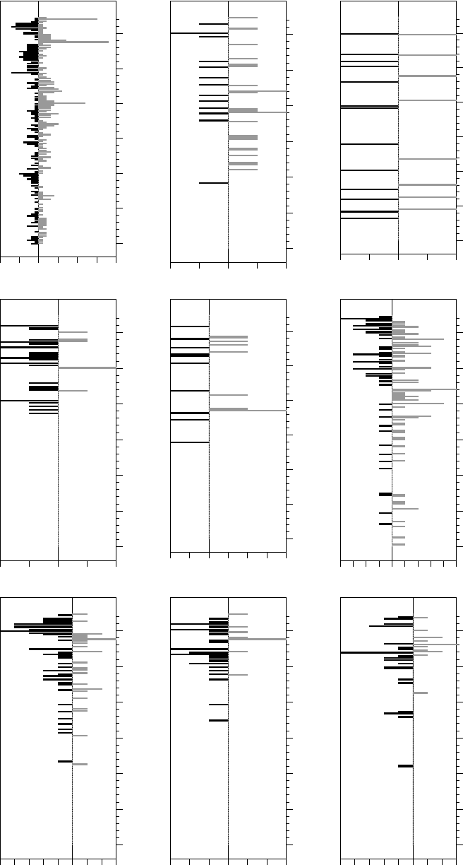
Figure 2: Credit and housing-related tax policies over time

loosening (negative) / tightening (positive)

Loan-to-value limits

1980 1985 1990 1995 2000 2005 2010

-3

-1

Debt service-to-income limits

1980 1985 1990 1995 2000 2005 2010

-3

-2

-1

Risk weighting

1980 1985 1990 1995 2000 2005 2010

-3

-1

Provisioning rules

1980 1985 1990 1995 2000 2005 2010

-2

-1

Exposure limits

1980 1985 1990 1995 2000 2005 2010

-2.0

-1.5

-1.0

-0.5

0.0

0.5

1.0

Housing-related taxes

1980 1985 1990 1995 2000 2005 2010

-5

-3

-1

Reserve requirements

1980 1985 1990 1995 2000 2005 2010

-20

-15

-10

-5

Liquidity requirements

1980 1985 1990 1995 2000 2005 2010

-2

-1

Credit growth

1980 1985 1990 1995 2000 2005 2010

-1.0

-0.5

0.0

0.5

1.0

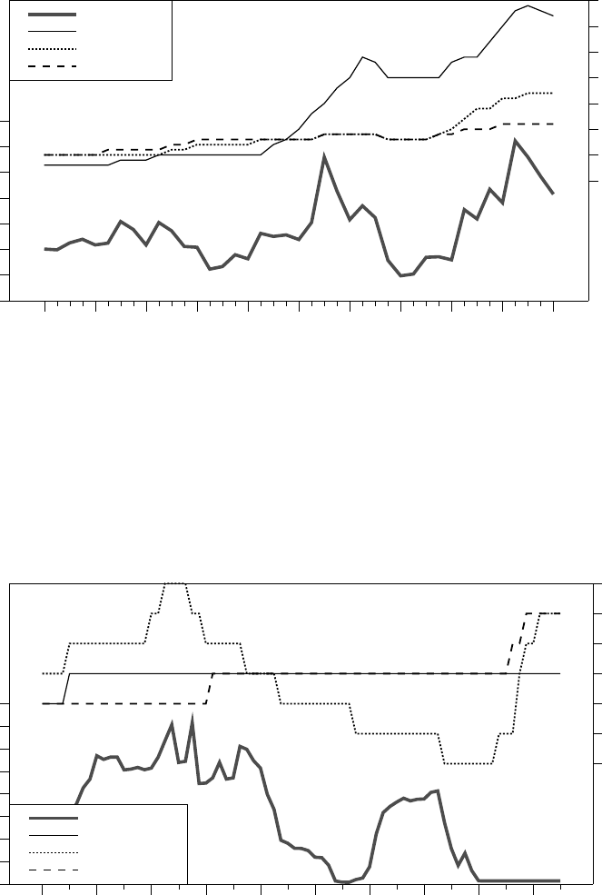
Figure 3: Interest rate and credit policies in China

interest'rate,'%

cumula/ve'/ghtening

2002 2003 2004 2005 2006 2007 2008 2009 2010 2011

Interest'rate

Reserve'Req

LTV

DSTI

Figure 4: Interest rate, credit and housing-related tax policies in Hong Kong SAR

interest'rate,'%

cumula/ve'/ghtening

1993 1995 1997 1999 2001 2003 2005 2007 2009 2011

Interest'rate

Credit'growth

Targeted'credit

Tax

Figure 5: Interest rate and credit policies in Korea

interest'rate,'%

cumula/ve'/ghtening

1986 1989 1992 1995 1998 2001 2004 2007 2010

Interest'rate

Reserve'Req

LTV

DSTI

Figure 6: Event study responses of housing credit to a general credit tightening

-30

-20

-10

Four-quarter growth rate

Notes: BG = Bulgaria; CO = Colombia; DE = Germany; EE = Estonia; FR = France; HK

= Hong Kong SAR; JP = Japan; KR = Korea; NZ = New Zealand; PL = Poland; TW =

Chinese Taipei.

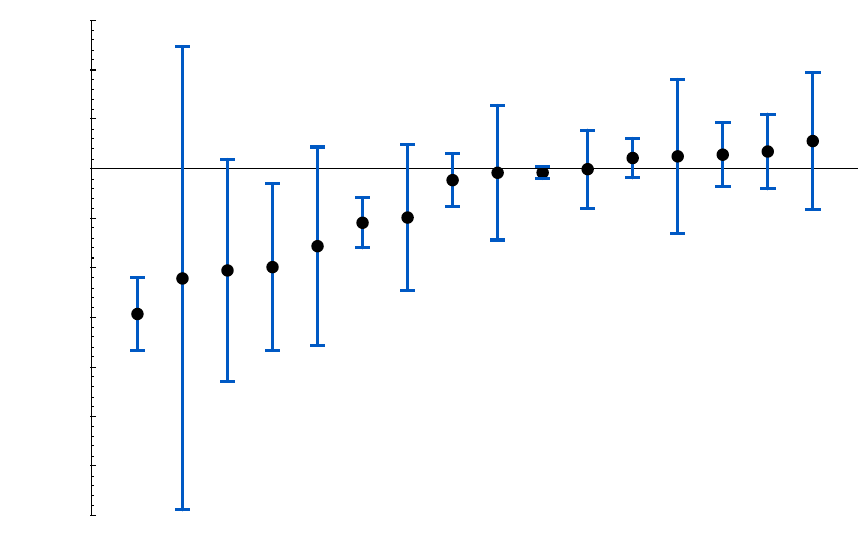
Figure 7: Event study responses of house prices to housing-related tax increases

-35

-30

-25

-20

-15

-10

-5

Four-quarter growth rate

Notes: CN = China; CZ = Czech Republic; DE = Germany; EE = Estonia; GR = Greece;

HK = Hong Kong SAR; HU = Hungary; IE = Ireland; JP = Japan; KR = Korea; MT =

Malta; MY = Malaysia; PL = Poland; SG = Singapore; TH = Thailand; US = United

States.

References

Bernanke, Ben S. 2010. Monetary Policy and the Housing Bubble. Speech delivered to the annual

meeting of the American Economic Association, January 3.

Bernanke, Ben S., & Gertler, Mark. 1999. Monetary Policy and Asset Price Volatility. Pages

77–128 of: New Challenges for Monetary Policy. Jackson Hole Symposium. Federal Reserve

Bank of Kansas City.

Blanchard, Olivier J., Dell’Ariccia, Giovanni, & Mauro, Paolo. 2010. Rethinking Macroeconomic

Policy. Journal of Money, Credit and Banking, 42, 199–215.

Borio, Claudio. 2011. Central Banking Post-Crisis: What Compass for Uncharted Waters? In:

Jones, Claire, & Pringle, Robert (eds), The Future of Central Banking. Central Bank

Publications.

Borio, Claudio, & Shim, Ilhyock. 2007. What Can (Macro-)prudential policy do to support

monetary policy? Working Paper 242. Bank for International Settlements.

Claessens, Stijn, Ghosh, Swati R., & Mihet, Roxana. 2013. Macro-Prudential Policies to Mitigate

Financial System Vulnerabilities. Journal of International Money and Finance, forthcoming.

Crowe, Cristopher, Dell’Ariccia, Giovanni, Igan, Deniz, & Rabanal, Pau. 2011. How to Deal with

Real Estate Booms: Lessons from Country Experiences. Working Paper 11/91. International

Monetary Fund.

Eichengreen, Barry, El-Erian, Mohamed, Fraga, Arminio, Ito, Takatoshi, Pisani-Ferry, Jean,

Prasad, Eswar, Rajan, Raghuram G., Ramos, Mara, Reinhart, Carmen M., Rodrik, Dani,

Rogoff, Kenneth S., Shin, Hyun Song, Velasco, Andr

es, & Yu, Yongding. 2011. Rethinking

Central Banking: Committee on International Economic Policy and Reform. The Brookings

Institution.

Gal

ı, Jordi. 2013. Monetary Policy and Rational Asset Price Bubbles. American Economic

Review, forthcoming.

Hilbers, Paul, Otker-Robe, Inci, Pazarbasioglu, Ceyla, & Johnsen, Gudrun. 2005. Assessing and

Managing Rapid Credit Growth and the Role of Supervisory and Prudential Policies. Working

Paper 05/151. International Monetary Fund.

IMF-BIS-Financial Stability Board. 2011 (October). Macroprudential Policy Tools and

Frameworks. Progress Report to G20.

Ito, Takatoshi. 2010. Monetary Policy and Financial Stability: Is Inﬂation Targeting Pass

Working Paper 206. Asian Development Bank.

King, Mervyn. 2013 (April). Monetary Policy: Many Targets, Many Instruments, Where Do We

Stand? Remarks at the IMF Conference on Rethinking Macro Policy II: First Steps and Early

Lessons.

Kuttner, Kenneth N. 2014. Low Interest Rates and Housing Bubbles: Still No Smoking Gun.

Chap. 8, pages 159–185 of: Evanoff, Douglas D. (ed), The Role of Central Banks in Financial

Stability: How Has It Changed? World Scientiﬁc, forthcoming.

Kuttner, Kenneth N., & Shim, Ilhyock. 2012. Taming the Real Estate Beast: The Effects of

Monetary and Macroprudential Policies on Housing Crices and Credit. Pages 231–259 of:

Heath, Alexandra, Packer, Frank, & Windsor, Callan (eds), Property Markets and Financial

Stability. Sydney: Reserve Bank of Australia.

Lim, Cheng Hoon, Columba, Francesco, Costa, Alejo, Kongsamut, Piyabha, Otani, Akira, Saiyid,

Mustafa, Wezel, Torsten, & Wu, Xiaoyong. 2011. Macroprudential Policy: What Instruments

and How to Use Them? Lessons from Country Experiences. Working Paper 11/238.

International Monetary Fund.

MacKinlay, A. Craig. 1997. Event Studies in Economics and Finance. Journal of Economic

Literature, 35(1), 13–39.

Mishkin, Frederic S. 2011. How should central banks respond to asset price bubbles? The ‘lean’

versus ’clean’ debate after the GFC. Reserve Bank of Australia Bulletin, June, 59–69.

Pesaran, M. Hashem, & Smith, Ron. 1995. Estimating Long-run Relationships from Dynamic

Heterogeneous Panels. Journal of Econometrics, 68(1), 79–113.

Posen, Adam S. 2006. Why Central Banks Should Not Burst Bubbles. International Finance,

9(1), 109–124.

Shim, Ilhyock, Bogdanova, Bilyana, Shek, Jimmy, & Subelyte, Agne. 2013. Database for Policy

Actions on Housing Markets. BIS Quarterly Review, September, 83–95.

Stein, Jeremy C. 2013 (February). Overheating in credit markets: Origins, measurement and

policy responses. Speech at the research symposioum on Restoring Household Financial

Stability After the Great Recession — Why Household Balance Sheets Matter? at the Federal

Reserve Bank of St. Louis.

Svensson, Lars E. O. 2010. Inﬂation Targeting. Chap. 22 of: Friedman, Benjamin M., &

Woodford, Michael (eds), Handbook of Monetary Economics, vol. 3B. North Holland.

Swamy, P. A. V. B. 1970. Efﬁcient Inference in a Random Coefﬁcient Regression Model.

Econometrica, 38(2), 311–323.

Tovar, Camilo, Garcia-Escribano, Mercedes, & Martin, Mercedes Vera. 2012. Credit Growth and

the Effectiveness of Reserve Requirements and Other Macroprudential Instruments in Latin

America. Working Paper 12/142. International Monetary Fund.

Vandenbussche, J

ome, Vogel, Ursula, & Detragiache, Enrica. 2012. Macroprudential Policies

and Housing Prices—A New Database and Empirical Evidence for Central, Eastern and

Southeastern Europe. Working Paper 12/303. International Monetary Fund.

Woodford, Michael. 2012 (April). Inﬂation Targeting and Financial Stability. Working Paper

17967. National Bureau of Economic Research.

Data appendix

Appendix Table 1: Coverage of the policy action dataset

Asia-Paciﬁc Australia China Hong Kong SAR India Indonesia

(1996/1998) (1998/1998) (1988/1991) (1998/1999) (2003/2008)

Japan Korea Malaysia New Zealand Philippines

(1999/1980) (2002/1988) (1989/1989) (1980/1980) (1980/1980)

Singapore Thailand Chinese Taipei

(1996/1996) (1999/1999) (2006/2000)

Central and Bulgaria Croatia Czech Republic Estonia Hungary

eastern Europe (1990/1990) (1997/1998) (1995/1990) (1993/1997) (2000/2000)

Latvia Lithuania Poland Romania Russia

(1992/2000) (1994/2000) (1997/2002) (1998/1998) (1998/1992)

Serbia Slovakia Slovenia Turkey Ukraine

(1999/2002) (1993/1995) (1996/2000) (1996/2002) (2001/2001)

Latin America Argentina Brazil Chile Colombia Mexico

(2000/2002) (1997/1994) (1991/1991) (1992/1999) (1999/2011)

Peru Uruguay

(2000/2000) (2001/2001)

Middle East Israel Saudi Arabia South Africa United Arab

and Africa (1999/1998) (1998/2007) (2001/1998) Emirates

(2001/2011)

North America Canada United States

(1985/1981) (1980/1980)

Western Europe Austria Belgium Denmark Finland France

(1998/1999) (1997/2000) (2003/2002) (1997/1987) (1997/1986)

Germany Greece Iceland Ireland Italy

(1982/1982) (1998/1999) (1997/1999) (1999/1981) (1984/1981)

Luxembourg Malta Netherlands Norway Portugal

(1999/1997) (1998/1990) (1998/1995) (1998/1980) (1996/1991)

Spain Sweden Switzerland United Kingdom

(1998/1999) (1997/1991) (1980/1988) (1980/1981)

Notes: The ﬁrst year listed in the brackets for each economy shows the ﬁrst year ofﬁcial source

materials from the monetary, prudential or ﬁscal authorities were reviewed to identify relevant

measures. The second year listed in the brackets shows the ﬁrst year a relevant policy action is

recorded in the dataset for each economy.

Appendix Table 2: Start and end dates for house price and housing credit data

House price Housing credit

Country Start End Start End Remarks

Argentina 2003Q1 2012Q1 2003Q1 2012Q2 Macro instability pre-2003

Austria 1993Q1 2012Q1 2003Q1 2011Q4 Extreme price volatility pre-1993

Australia 1980Q1 2012Q1 1980Q1 2012Q2

Belgium 1980Q1 2011Q4 1980Q1 2012Q2

Bulgaria 2001Q1 2012Q1 2001Q1 2012Q2 Macro instability pre-2001

Brazil 2010Q4 2012Q1 1997Q1 2012Q2 Extreme credit volatility

Canada 1980Q1 2012Q1 1980Q1 2012Q2

Switzerland 1980Q1 2012Q1 1980Q1 2012Q2

Chile 1990Q4 2007Q4 2001Q1 2012Q2

China 2001Q1 2011Q4 2001Q1 2011Q4 Extreme price & credit volatility

Colombia 1988Q1 2011Q2 1994Q4 2012Q2

Czech Republic 1999Q1 2010Q4 1997Q1 2012Q2

Germany 1980Q1 2011Q4 1980Q4 2012Q2

Denmark 1980Q1 2011Q4 2003Q1 2012Q2

Estonia 2002Q1 2012Q1 2002Q1 2011Q4 Macro instability pre-2002

Spain 1987Q1 2012Q1 1989Q1 2012Q1

Finland 1980Q1 2012Q1 1989Q2 2012Q2

France 1994Q4 2011Q4 1980Q1 2012Q2

Great Britain 1980Q1 2011Q4 1980Q1 2012Q1

Greece 1993Q4 2012Q1 1980Q1 2012Q2

Hong Kong SAR 1993Q1 2012Q1 1981Q4 2012Q2

Croatia 1998Q1 2010Q4 1999Q3 2012Q2 Macro instability pre-1998

Hungary 2001Q4 2012Q1 1993Q1 2012Q2 Large spike in credit data

Indonesia 2000Q1 2012Q1 2000Q1 2012Q2 Macro instability, Asian crisis

Ireland 1980Q1 2011Q4 1990Q3 2012Q2

Israel 1994Q1 2011Q4 2004Q1 2011Q1 Extreme ﬁrst credit observation

India 2003Q2 2012Q1 1998Q4 2011Q4

Iceland 2000Q1 2012Q1 2009Q1 2012Q1 Credit fell by half during crisis

Italy 1991Q1 2011Q4 1998Q2 2012Q2

Japan 1980Q1 2011Q4 1980Q1 2012Q1

Korea 1986Q1 2012Q1 1996Q1 2012Q2

Lithuania 1998Q4 2011Q4 2004Q1 2012Q2

Luxembourg 1980Q1 2011Q4 1999Q1 2012Q2

Latvia 2006Q1 2011Q4 2003Q3 2012Q2

Malta 2000Q1 2011Q4 1996Q1 2012Q2

Mexico 2005Q1 2012Q1 1996Q4 2012Q2

Malaysia 1999Q1 2011Q4 1996Q4 2012Q2

Netherlands 1985Q1 2012Q1 1990Q4 2012Q2 Extreme price volatility pre-1985

Norway 1991Q1 2012Q1 1991Q3 2012Q2

New Zealand 1980Q1 2011Q4 1998Q2 2012Q2

Continued on next page

House price Housing credit

Country Start End Start End Remarks

Peru 2002Q1 2012Q1 2002Q1 2012Q2 Macro instability pre-2002

Philippines 1981Q1 2011Q4 2001Q3 2012Q1 Extreme ﬁrst two credit observations

Poland 2002Q4 2012Q1 1996Q4 2012Q2

Portugal 1988Q1 2012Q1 1980Q1 2012Q2

Romania 2005Q4 2011Q4 2007Q1 2012Q2

Serbia 2003Q2 2011Q4 2008Q2 2012Q2

Russia 2001Q1 2011Q4 2004Q2 2012Q2

Sweden 1993Q1 2012Q1 2001Q4 2012Q2

Singapore 1980Q1 2012Q1 1991Q1 2012Q2

Slovenia 2003Q1 2011Q4 2005Q2 2012Q2 Extreme ﬁrst two credit observations

Slovakia 2005Q1 2012Q1 2006Q1 2012Q2

Thailand 1999Q1 2011Q2 1999Q1 2012Q2 Macro instability, Asian crisis

Turkey 2007Q2 2011Q4 2007Q1 2012Q2 Large spike in credit data

Chinese Taipei 1991Q3 2011Q3 1988Q3 2012Q2

Ukraine 2000Q2 2012Q1 2006Q1 2012Q2

United States 1980Q1 2012Q1 1980Q1 2012Q1

South Africa 1980Q1 2012Q1 1980Q1 2012Q2

Notes: Italicized entries are those for which the starting date was moved up to exclude extreme or

highly volatile observations. The shaded grey entries are dropped from the regressions because of

insufﬁcient data.