
Lecture 10:
Controllability and
Observability
2018 Autumn
1

Contents
Introduction
Controllability
Observability
Canonical Decomposition
Conditions in Jordan-Form Equations
Discrete-Time State-Space Equations
Controllability After Sampling
LTV State-Space Equations
2

Controllability and observability
We will discuss two fundamental concepts of system
theory:
controllability
observability
These two concepts describe the interaction in a
system between the external world (inputs and
outputs) and the internal variables (states).
3

Loosely speaking,
Controllability is the property that indicates if the
behaviour of a system can be controlled by acting on
its inputs.
Observability is the property that indicates if the
internal behaviour of a system can be
observed/detected/estimated at its outputs.
4
Controllability and observability

Controllability
5

Consider an LTI system represented by the following
state equation with n states and p inputs
(t) = Ax(t) + Bu(t)
where AR
nn
and BR
np
.
Controllability only relates inputs and states, thus the
output equation y(t) = Cx(t) + Du(t) is irrelevant.
6
Controllability

Controllability: definition
Controllability:
The state equation or the pair (A, B) is said to be
controllable if for any initial state x(0) = x
0
and any final
state x
1
, there exists an input that transfers x
0
to x
1
in a finite
time.
If an input to a system can be found that takes every state
variable from a desired initial state to a desired final state,
the system is said to be controllable.
A system is completely controllable if there exists an
unconstrained control u(t) that can transfer any initial state
x(t
0
) to any other desired location x(t) in a finite time, t
0
to t
1
.
The closed-loop system pole locations can be arbitrarily
placed if and only if the system is controllable.
7

Otherwise, the state equations or the pair (A, B) is
said to be uncontrollable.
This definition requires only that the input be capable
of driving the state anywhere in the state space in a
finite time; what trajectory the state takes is not
specified.
8
Controllability: definition

Examples: Uncontrollable systems
If the capacitor has no initial charge, or x(0) = 0, then x(t) = 0
for all t 0, no matter what input is applied.
The input has no effect over the voltage across the capacitor.
This system, or more precisely, a state equation that describes
it, is not controllable.
9

The system has two state variables.
The input can transfer x
1
(t) or x
2
(t) to any desired
value, but no matter what input is applied, x
1
(t) will
always equal x
2
(t).
This system is not
controllable either.
10
Examples: Uncontrollable systems

Theorem: Controllability Tests
The following statements are equivalent.
1. The n-dimensional pair (A, B) is controllable.
2. The controllability matrix
= [B AB A
2
B ... A
n-1
B]
has rank n (full row rank).
3. The nn matrix
is nonsingular for all t > 0.
11

Example
The linearised state space equation of an inverted
pendulum system is given by
12

We compute the controllability matrix
= [B AB A
2
B A
3
B] =
which has rank 4 (i.e., it is full rank).
Hence, the system is controllable.
This can also be done in Matlab.
If were slightly different from 0, we know then that
there exists a control u(t) that will return it to the
equilibrium in finite time.
13
0 1 0 0
1 0 2 0
0 2 0 10
2 0 10 0
Example

Controllability and Algebraic Equivalence
Controllability is a system property that is invariant
with respect to algebraic equivalence transformations
(change of coordinates).
Consider the pair (A, B) with controllability matrix
= [B AB A
2
B ... A
n-1
B]
and an algebraic equivalent pair (
,
), where
= PAP
-1
and
= PB, and P is a nonsingular
matrix ( = Px) – see slide 40 from Lecture 7.
14

Then the controllability matrix of the pair (
,
) is
rank = rank
(because P is nonsingular).
15
Controllability and Algebraic Equivalence

T
t
Aτ TAτ
c
0
W t e BB e dτ
Controllability Gramian
The matrix W
c
(t), introduced to check controllability
of (A, B), can be used to construct an open loop
control signal u(t) that will take the state x from any
x
0
to any x
1
in finite time.
16

Controllability Gramian
The corresponding control law is given by
This control law uses the least amount of energy to
transfer x from x
0
to x
1
in time t
1
.
This means that for any other control (t) performing
the same transfer,
17
T
1
1
A t t
At
T1
C 1 0 1
u t B e W t e x x
11
tt
22
00
u τ dτ u τ dτ

Controllability Gramian
For example, if x
0
= 0, the minimum control energy is
18

Controllability Gramian
If the matrix A is Hurwitz (all eigenvalues have
negative real parts), then W
c
(t) converges to a
constant W
c
as t; hence, controllability gramian
becomes
W
c
is called the Controllability Gramian of (A, B).
19

Controllability Gramian
If we desire to drive the state x from 0 to x
1
in infinite
time t
1
, we find that the least required control
energy would be
Note that the closer to zero any eigenvalue of W
c
is,
the closer to singular would W
c
be, and the larger
would be the minimum energy required to drive the
state to x
1
.
20

Controllability Gramian
We do not need to solve an infinite integral to
compute W
c
.
If (A, B) is controllable (i.e., has full row rank), W
c
is the unique solution of the linear Lyapunov matrix
equation
AW
c
+W
c
A
T
= BB
T
which can be solved with MATLAB.
21

Example 6.3
22
0.5 0 0.5
x x u
0 1 1
0.5 0.25
ρ B AB ρ 2
11

Example 6.3
23
T
1
t
Aτ TAτ
C1
0
-0.5τ -0.5τ
2
C
-τ -τ
0
W t = e BB e dτ
0.5
e 0 e 0
W 2 = 0.5 1 dτ
1
0 e 0 e
0.2162 0.3167
=
0.3167 0.4908

Example 6.3
24
T
1
1
A t t
t
T1
C 1 0 1
0.5 2 t
1
1
1C
2
2t
0.5t t
u t = B e W t e x x
e 0 10
e0
u t = 0.5 1 W 2
1
0e
0e
= 58.82e + 27.96e

Example 6.3
25


Observability
27

Luenberger observer
28

Concept of observability
The concept of observability is dual to that of
controllability, and deals with the possibility of
estimating/observing the state of the system from the
knowledge of its inputs and outputs.
Consider the LTI system
(t) = Ax(t) + Bu(t), x(t)R
n
, u(t)R
q
y(t) = Cx(t) + Du(t), y(t)R
p
29

Concept of observability
Observability:
The state equation (SE), or the pair (A, C), is said to be
observable if for any unknown initial state x(0), there exists
a finite time t
1
> 0 such that the knowledge of the input u(t)
and the output y(t) over [0, t
1
] suffices to determine
uniquely the initial state x(0); otherwise, the equation is said
to be unobservable.
If the initial-state vector, x(t
0
), can be found from u(t) and
y(t) measured over a finite interval of time from t
0
, the
system is said to be observable; otherwise, the system is
said to be unobservable.
30

Concept of observability
Observability:
A system is completely observable if and only if there exists
a finite time T such that the initial state x(0) can be
determined from the observation history y(t) given the
control u(t), t
0
to T.
Observability refers to the ability to estimate a state variable.
31

Example: Unobservable systems
The network has two state variables: the current x
1
through the inductor and the voltage x
2
across the
capacitor; the input u is a current source.
32

Example: Unobservable systems
If u = 0, x
2
(0) = 0 and x
1
(0) = a 0, then the output is
identically zero.
Any x(0) = [a 0]
T
and u(t) = 0, for t 0, yield the
same output y(t) = 0.
Thus, there is no way to uniquely determine the initial
state [a 0]
T
; thus, the system is unobservable.
33

Analysis with the output solution
We have shown that the response of the state equation
system is given by
In studying observability, we assume u and y are
known; the initial state x(0) is unknown.
From the previous equation,
Ce
At
x(0) = (t), where
34

Analysis with the output solution
(t) is a known function.
Thus the observability problem reduces to finding x(0)
as the unique solution of Ce
At
x(0) = (t).
For a fixed time t, Ce
At
is a pn real, constant matrix,
and (t) is a constant p1 vector.
Thus, in general, because p < n (there are less outputs
than states) we cannot find a unique vector x(0) from
Ce
At
x(0) = (t) for a given fixed t; that is, we have
more unknowns n than equations, p.
To determine x(0) uniquely, we need to use the
knowledge of y(t) and u(t) over a nonzero time
interval.
35

Observability Gramian
Theorem (Observability Gramian Test): The state
equation (SE) is observable if and only if the nn
matrix
is nonsingular for any t > 0.
Observability only depends on the matrices A and C.
36

Observability Gramian
If the matrix A is Hurwitz (all eigenvalues have
negative real part), then W
o
(t) converges for t,
and we simply denote it by W
o
:
W
o
is called the Observability Gramian of (A, C).
37
cf>

Compute Observability Gramian
Observability Gramian can be computed by solving
the linear matrix Lyapunov equation
W
o
A + A
T
W
o
= -C
T
C:
By checking the rank of the observability matrix O
(dual of ) or W
o
, we can determine if a pair (A, C) is
observable.
38

Duality of Controllability and Observability
Recall that controllability and observability are dual.
Theorem (Duality): The pair (A, B) is controllable if
and only if the pair (A
T
, B
T
) is observable.
39

Proof: The pair (A, B) is controllable if and only if
is nonsingular for any t. On the other hand, the pair (A
T
,
B
T
) is observable if and only if,
is nonsingular for any t. (We replace A by A
T
and C by
B
T
in observability Gramian.)
The two conditions are thus identical. QED
40
Duality of Controllability and Observability

The duality between controllability and observability
establishes that we can test the observability of a pair
(A,C) by using the controllability tests, which we
already know, on the pair (A
T
,C
T
).
41
Duality of Controllability and Observability

Example: Observability Test
By duality, we can check the observability of this
system as the controllability of (A
T
,C
T
) for instance,
via the matrix
which has rank 3.
Hence (A,C) is observable.
42

Theorem: Observability Tests
The following statements are equivalent.
1. An LTI system with the n-dimensional pair (A,C),
where AR
nn
and CR
pn
, is observable.
2. The Observability Matrix OR
npn
has rank n (full column rank).
43

Theorem: Observability Tests
3. The nn matrix W
o
(t)
is nonsingular for all t > 0.
44

Observability Examples
A linearised state equation for a satellite in circular
orbit is given by
where the first output is the (incremental) radial
distance r(t) and the second the (incremental) angle (t).
45

Observability Examples
The position of the satellite can be adjusted by means
of the thrust forces u
1
(t) and u
2
(t).
The nominal radius is r
0
and the nominal angular
velocity
0
.
Suppose that only radial distance measurements
y
1
(t) = [1 0 0 0]x(t) = C
1
x(t)
are available on a specified time interval.
46
https://youtu.be/xLu0Ak9Blog

Observability Examples
The observability matrix O is
Rank O = 3; therefore, radial measurement does not
suffice to compute the complete orbit state.
On the other hand, measurement of angle,
y
1
(t) = [0 0 1 0]x(t) = C
2
x(t)
does suffice, as can be readily verified.
47
1
1
3
2
0 0 0
1
2
3
0
1
1 0 0 0
C
0 1 0 0
CA
=
3ω 0 0 2r ω
CA
0 ω 00
CA

RLC circuit
The RLC circuit is modelled by the following state
equation
48
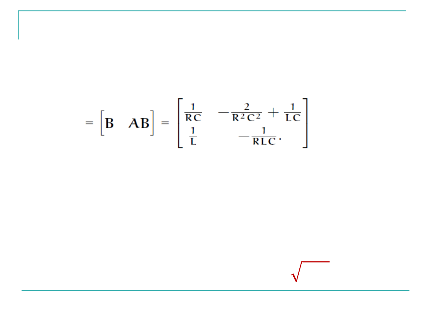
RLC circuit
We test controllability by checking the rank of the
controllability matrix .
The rank of this matrix can be checked with the
determinant
det = 1/[R
2
LC
2
] – 1/[L
2
C]
The determinant is zero, i.e., the system is
uncontrollable, if
1/[R
2
LC
2
] – 1/[L
2
C] = 0 R =
49

RLC circuit
On the other hand, the observability matrix O is
which is obviously full rank.
Hence the RLC circuit is always observable, but
becomes uncontrollable whenever R = .
50

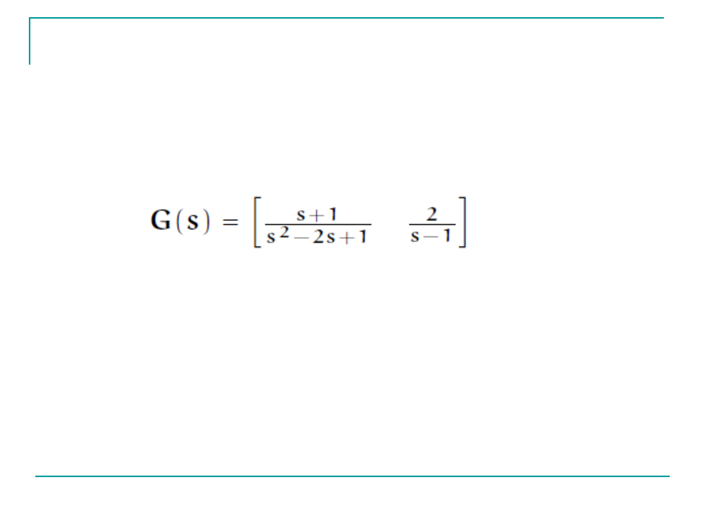
RLC circuit
What happens to the system transfer function when
controllability is lost?
The calculation, using the known formula
G(s) = C(sI A)
-1
B + D,
gives
51

RLC circuit
The poles of the circuit transfer function are
Both roots have negative real part, and thus we
conclude that the system is asymptotically stable and
BIBO stable for any value of R, L and C.
52

RLC circuit
In particular, for R= (the value for which the
system becomes uncontrollable), we have
s
1,2
= 1/[RC]
The system has repeated roots, and
A pole-zero cancellation reduces the system to first
order.
53

Minimum Realisation
A system is irreducible if and only if it is both
controllable and observable.
An irreducible system is called the minimal
realisation.
Hence, the system can be reduced to a lower order.
54

Canonical Decompositions
55

Canonical Decompositions
The canonical decompositions of state space
equations establish the relationship between
controllability, observability, transfer matrix and
minimal realisations.
56
Controllability & Observability
Realisation (A, B, C, D)

Review: controllable canonical form
i
: coefficient of the denominator of G(s)
i
: coefficient of the numerator of G(s)
() = rank[B AB ... A
n-1
B]= n
57

Review: solution to DT state eqns
The solution of the discrete-time state equations is
considerably simpler that that of continuous-time
state equations. From
x[k + 1] = Ax[k] + Bu[k],
we have
x[1] = Ax[0] + Bu[0]
x[2] = Ax[1] + Bu[1] = A
2
x[0] + ABu[0] + Bu[1]
...
58

Review: solution to DT state eqns
By proceeding forward, we readily obtain for k > 0
59

Review: Similarity Transformation
x(t)R
n
, u(t)R
p
, y(t)R
q
(t) = Ax(t) + Bu(t)
y(t) = Cx(t) + Du(t)
Let =Px, where PR
nn
is nonsingular. Then,
(t) =
(t) +
u(t)
y(t) =
(t) +
u(t)
is algebraically equivalent to (A, B, C, D), where
=PAP
-1
,
=PB,
=CP
-1
, and
=D.
60

Controllable/Uncontrollable Decomposition
Theorem 6.6: Consider the n-dimensional state
equation (A,B,C,D) and suppose
() = rank[B AB ... A
n-1
B] = n
1
< n
i.e., the system is uncontrollable.
Let the nn matrix of change of coordinates P be
defined as
P
-1
= [q
1
q
2
... q
n
1
... q
n
]
where the first n
1
columns are any n
1
independent
columns in , and the remaining are arbitrarily chosen
so that P is nonsingular.
61

Then the equivalence transformation =Px transforms
(A, B, C, D) to
62
Controllable/Uncontrollable Decomposition

The states in the new coordinates are decomposed
into
C
: n
1
controllable states
: n n
1
uncontrollable states
63
decoupled from
the input u
Controllable/Uncontrollable Decomposition

The reduced order state equation of the controllable
states
(t) =
(t) +
u(t)
y(t) =
(t) + Du(t)
is controllable and has the same transfer function as the
original state equation (A, B, C, D).
Pole-zero cancellation occurs in deriving the transfer
function.
64
Controllable/Uncontrollable Decomposition

Example: Controllable Decomposition
Consider the third order system
Compute the rank of the controllability matrix
() = rank[B AB A
2
B] =
= 2 < 3
Uncontrollable!
65
0 1 1 1 2 1
rank 1 0 1 0 1 0
0 1 1 1 2 1

Take the change of coordinates P
-1
formed by the first
two columns of and an arbitrary third one that is
independent of the first two.
Remind>
=
66
Example: Controllable Decomposition

Setting = Px we obtain the equivalent equations
and the reduced controllable system
67
Example: Controllable Decomposition
A simple computation shows that the three state space
equations have the same transfer matrix.
68
Example: Controllable Decomposition

Summary
Today, we have learnt
Controllability
Controllability matrix
Observability
Observability matrix O
Controllability and Observability Gramian
Controllability Decomposition
Next week, we will continue with
Observable/Unobservable Decomposition
Kalman Decomposition
Next Chapter: State Feedback and State Estimators
69

There will be no lecture on 2018-11-21.
70
Lecture Cancellation
