Closing Costs, Refinancing, and Inefficiencies in the Mortgage Market

Closing Costs, Reﬁnancing, and Ineﬃciencies

in the Mortgage Market

David Zhang

∗

Rice University

(Click here for latest version)

February 3, 2023

Abstract

I use a structural model to quantify the cross-subsidization in the US mortgage

market due to heterogeneous borrower reﬁnancing tendencies. Actively reﬁnancing

borrowers gain up to 3% of their loan amount relative to non-reﬁnancing borrowers in

expectation. In equilibrium, the presence of borrowers with high reﬁnancing inertia

reduces mortgage interest rates particularly on lower upfront closing cost mortgages

which have more valuable reﬁnancing options. As a result, actively reﬁnancing bor-

rowers reﬁnance excessively relative to a perfect information, no cross-subsidization

benchmark, an eﬀect that accounts for around 28% of the overall reﬁnancing volume

and generates signiﬁcant deadweight losses due to administrative resource costs. Alter-

native contract designs can simultaneously reduce transfers and increase total welfare.

∗

I thank John Campbell, Ed Glaeser, Adi Sunderam, Ariel Pakes, and Robin Lee for continuous advice

on this paper. I also thank Jo˜ao Cocco, Matthew Curtis, Mark Egan, Xiang Fang, Jiacheng Feng, Xavier

Gabaix, Daniel Green, Shiyang Huang, Jun Ishii, Larry Katz, Amir Kermani, Alex Kopytov, David Laibson,

Doug McManus, Konstantin Milbradt, Fabrice Tourre, Pascal Noel, Henry Overman, Frank Pinter, David

Scharfstein, Jeremy Stein, Dragon Tang, Audrey Tiew, Fabrice Tourre, Boris Vallee, Nancy Wallace, Jeﬀrey

Wang, Paul Willen, Ron Yang, and seminar/conference participants at CityUHK, HKU, TAMU, SMU, BC,

UofT, Purdue, Rice, Fed Board, Minnesota, CU Boulder, 2022 Chicago Booth Household Finance Conference,

2022 NBER Summer Institute Real Estate, 2022 North American Summer Meeting of the Econometric

Society, 2022 Asian Meeting of the Econometric Society, and 2023 ASSA/AREUEA Meeting for valuable

comments which greatly improved the paper. All errors are my own. This research was conducted while the

author was a Visiting Fellow at the Federal Reserve Bank of Boston. The views expressed in this paper are

solely those of the author and not necessarily those of the Federal Reserve Bank of Boston nor the Federal

Reserve System.

1 Introduction

In the US, many borrowers are slow to reﬁnance, or never reﬁnance, their mortgages when

interest rates fall, while others are more quick at doing so. This heterogeneity in reﬁnancing

inertia which has long been recognized as an important friction in household ﬁnance.

this paper, I use a structural model to quantify the distributional and eﬃciency implications

of the heterogeneous consumer reﬁnancing inertia.

My model identiﬁes two main channels through which heterogeneous consumer reﬁnanc-

ing inertia aﬀects on the US mortgage market. First, the existence of borrowers with reﬁ-

nancing inertia implies that lenders can aﬀord to charge lower interest rates upfront. This

interest rate reduction eﬀect reﬂects a cross-subsidization from slow to reﬁnance borrowers

to the more quick to reﬁnance borrowers. Second, I identify a non-uniformity of the interest

rate reduction eﬀect across upfront closing cost choices which distorts borrower contract

choice, further increases cross-subsidization, and generates economic ineﬃciencies. In par-

ticular, the interest rate reduction eﬀect is particularly large for lower upfront closing cost

mortgages, which generates excessive reﬁnancing by quick to reﬁnance borrowers leading to

deadweight administrative costs.

By way of background, mortgage originating lenders must cover their costs. They can do

so in two ways. First, they can charge the borrower upfront, though upfront closing costs.

Second, they can raise the interest rate on the mortgage, holding ﬁxed its principal balance

and then recovering their costs from the secondary market. Most lenders oﬀer a menu of

rate and upfront closing cost options to prospective borrowers through a choice of how many

“points” to pay to or receive from the lender.

Borrowers therefore have a choice of getting

a lower rate, higher upfront closing cost mortgage, or a higher rate, lower upfront closing

See, e.g., Schwartz and Torous (1989), Archer and Ling (1993), McConnell and Singh (1994), Stanton

(1995), Green and LaCour-Little (1999), Campbell (2006), Agarwal, Rosen, and Yao (2016), Keys, Pope,

and Pope (2016), Johnson, Meier, and Toubia (2018), Andersen, Campbell, Nielsen, and Ramadorai (2018),

and Gerardi, Willen, and Zhang (2021).

In the industry, each mortgage point refers to 1% of the loan amount that borrowers pay upfront. Positive

points in the form of discount points increase the upfront closing cost while reducing the interest rate, while

negative points the form of lender credit to reduce upfront closing cost while increasing the interest rate.

cost mortgage.

Higher rate, lower upfront closing cost mortgages by construction carry a more valuable

reﬁnancing option compared to lower rate, higher upfront closing cost mortgages, and I show

that their prices are more aﬀected by the existence of borrowers with reﬁnancing inertia in

equilibrium. This incentivizes actively reﬁnancing borrowers to reﬁnance more often than

they otherwise would, due to two mechanisms. First, actively reﬁnancing borrowers become

less likely to pay points to reduce their rate, and end up with mortgages with a higher

reﬁnancing incentive.

Second, actively reﬁnancing borrowers are able to reﬁnance more fre-

quently than they otherwise would by taking out a lower upfront closing cost mortgage when

they do reﬁnance. Note that these mechanisms involve changes in the actively reﬁnancing

borrowers’ upfront closing cost choices and expected reﬁnancing activity, rather than their

levels. Because mortgage reﬁnancing involves administrative resources that could have been

used for other economic activity, the extra reﬁnancing that quick to reﬁnance borrowers

undertake solely to receive transfers generates deadweight losses from a social perspective.

To quantify the size of the cross-subsidy by borrower reﬁnancing tendencies and study

its eﬃciency consequences, I develop a structural equilibrium model that captures borrower

heterogeneity in reﬁnancing and moving tendencies while endogenizing borrower choices

of upfront closing costs. To do so, I embed the time and state dependence of borrower

reﬁnancing behavior described in Andersen, Campbell, Nielsen, and Ramadorai (2020) into

a life-cycle model that gives welfare estimates interpretable in dollar-equivalent terms. A

zero-proﬁt condition with a Monte Carlo model of mortgage-backed securities pricing pins

down the supply side.

Borrowers in my model are heterogeneous in terms of their (i) reﬁnancing costs, includ-

ing a time-varying ability to reﬁnance and a hassle cost conditional on them being able to

This is consistent with Dave Ramsey’s ﬁnancial advice, which says that: “most buyers won’t regain their

money on mortgage points because they usually reﬁnance, pay oﬀ, or sell their homes before they reach their

break-even point.” Source: https://www.ramseysolutions.com/real-estate/what-are-mortgage-points. This

ﬁnancial advice turns out to be correct for my benchmark optimally reﬁnancing borrower, but only due to

the cross-subsidization from slow to reﬁnance borrowers.

reﬁnance, (ii) moving or exogenous prepayment probabilities, (iii) discount factors, and (iv)

liquid wealth and income. The time-varying ability to reﬁnance and the reﬁnancing has-

sle cost are separately identiﬁed from borrower delays in reﬁnancing after their reﬁnancing

thresholds has been reached (Andersen et al., 2020), and could reﬂect both demand-side dif-

ferences in preferences as well as any supply-side driven diﬀerential costs to reﬁnance coming

from potential discrimination in the market. Moving or exogenous prepayment probabilities

are identiﬁed based on prepayment during periods of low interest rate incentives. Discount

factors are identiﬁed based on choices of upfront closing costs. Borrowers’ liquid wealth and

income are calibrated using data from the Survey of Consumer Finances (SCF).

I estimate the model using maximum likelihood on a novel data set linking borrower up-

front closing cost choices to their subsequent prepayment behavior. Three main conclusions

emerge from my empirical work. First, cross-subsidization from slow-to-reﬁnance borrowers

signiﬁcantly aﬀects equilibrium prices and is larger on mortgages with lower upfront closing

costs. For a calibrated borrower who is always able to reﬁnance at a hassle cost of $200, a

mortgage with a one percent upfront closing cost carries a 0.97% lower interest rate in the

existing market equilibrium relative to a world without cross-subsidization. For mortgages

with a four percent upfront closing cost, the diﬀerence is smaller at 0.21%. The intuitive

reason for the larger cross-subsidization of lower upfront closing cost mortgages is that, from

the perspective of the lender, slow to reﬁnance reﬁnance borrowers overpay for their mort-

gage closing costs when they pay it through the rate because they keep paying the higher

interest rate for longer.

A key advantage of my approach is that I am able to quantify the consequences of this

cross-subsidization. The economic consequences of this are signiﬁcant. As my second con-

clusion, I ﬁnd that the cross-subsidization of mortgage closing costs generates large transfers

between borrowers. Black and Hispanic borrowers are particularly worse oﬀ in the pooling

equilibrium. As my third conclusion, I show that the eﬃciency consequences of price distor-

tions are large. In particular, I estimate that around one quarter of all US reﬁnancing would

not have occurred but for this cross-subsidization, leading to a welfare loss of around $3.5

billion per year relative to the no cross-subsidization benchmark.

Using the model, I conduct two counterfactual analyses. First, I investigate borrower

welfare under an alternative contract design where their closing costs have to be added to

the mortgage balance. I ﬁnd a reduction in cross-subsidization from $1339/borrower to

$698/borrower, a decrease of 48%. Furthermore, I ﬁnd an increase in average borrower

utility of $556/borrower in dollar terms. Second, I study the case of automatically reﬁ-

nancing mortgages. This contract eliminates the cross-subsidization between borrowers with

diﬀerent reﬁnancing speeds, and leads to a bigger increase in average borrower utility of

$1215/borrower. My results suggests that the equity-eﬃciency trade-oﬀ is not binding in

the US mortgage context: it is possible to reduce inequality while increasing total welfare.

My model generates cross-sectional in borrower reﬁnancing behavior through hetero-

geneous reﬁnancing costs that could come from either the demand or supply side and is

consistent with all borrowers being rational. Nevertheless, if one instead views the slow to

reﬁnance borrowers as behavioral agents who do not understand the true cost of a higher

interest rate, it can also be interpreted as an empirical model of a shrouded equilibrium as

in Gabaix and Laibson (2006) where the quick to reﬁnance borrowers select against the slow

to reﬁnance borrowers. Since I focus on the dollar value consequences of heterogeneous reﬁ-

nancing behavior and the value of alternative contract designs, my conclusions are invariant

to either interpretation.

My paper is related to the literature on borrower heterogeneity in mortgage reﬁnancing

behavior. Many papers document large borrower heterogeneity in reﬁnancing behavior con-

ditional on the interest rate savings available, including Archer and Ling (1993), McConnell

and Singh (1994), Stanton (1995), Deng, Quigley, and Van Order (2000), Agarwal, Rosen,

and Yao (2016), Keys, Pope, and Pope (2016), Johnson, Meier, and Toubia (2018), Andersen

et al. (2018), Beraja, Fuster, Hurst, and Vavra (2018), Ambokar and Samaee (2019), Bel-

gibayeva, Bono, Bracke, Cocco, and Majer (2020), and Gerardi, Willen, and Zhang (2021).

Most of this literature has studied this heterogeneity in the reduced form, and none quanti-

ﬁes the cross-subsidization across borrowers with diﬀerent reﬁnancing tendencies in market

equilibrium and studies its eﬃciency implications.

More closely related to my paper are Fisher, Gavazza, Liu, Ramadorai, and Tripathy

(2022) and Berger, Milbradt, Tourre, and Vavra (2023), which uses structural models to

study reﬁnancing heterogeneity and cross-subsidization in the UK and US mortgage mar-

ket, respectively. Neither studies the ineﬃciencies generated by this cross-subsidization due

to distortions in the choices of quick to reﬁnance borrowers, which is the main conceptual

contribution of this paper. I show that these ineﬃciencies are economically important and

presents a reason to consider alternative contract designs beyond redistribution. Further-

more, I compute results by race and ethnicity and show that their expected loss under the

current US system relative to a no cross-subsidization benchmark is sizable even in an ex

ante sense.

My paper also contributes to the literature on life-cycle models of mortgage choice. This

includes Campbell and Cocco (2003), Mayer, Piskorski, and Tchistyi (2013), Corbae and

Quintin (2015), Campbell and Cocco (2015) Eichenbaum, Rebelo, and Wong (2018), Chen,

Michaux, and Roussanov (2020), Campbell, Clara, and Cocco (2021), Guren, Krishnamurthy,

and McQuade (2021) and MacGee and Yao (2022). My model builds in both state and time

dependence in reﬁnancing costs in a life-cycle model of mortgage choice with endogenous

mortgage premia. Of these papers, only Eichenbaum, Rebelo, and Wong (2018) incorporate

equilibrium cross-sectional heterogeneity in reﬁnancing behavior, which they use to model the

state-dependent behavior of monetary policy, but they do not endogenize the mortgage pre-

mia and subsequently do not study its implications in terms of borrower cross-subsidization

and eﬃciency.

In terms of institutions, my paper is related to a growing literature on choices of mortgage

upfront closing costs, which are also called points. In this literature, Brueckner (1994) LeRoy

(1996), and Stanton and Wallace (2003) present theories of mortgage points that emphasize

the role of selection on borrowers’ expected prepayment speeds. My empirical work takes the

selection eﬀect explored in these theories seriously and evaluates their welfare implications

under heterogeneous reﬁnancing tendencies. Chari and Jagannathan (1989) studies the role

of insurance to income shocks for the institution of mortgage points, which I also incorporate

in my quantitative model. Empirical work on consumer behavior with mortgage points

includes Woodward and Hall (2012) who document how points may lead to sub-optimal

shopping, Agarwal, Ben-David, and Yao (2017) who show that many borrowers make the

“mistake” of paying too much in points given their predicted reﬁnancing propensities, and

Benetton, Gavazza, and Surico (2020) who look at the UK context and ﬁnds that lenders

may exploit heterogeneity in demand elasticities between rates and points to increase proﬁts.

Another strand of literature on mortgage points focuses its role in mortgage discrimination,

including Bhutta and Hizmo (2019), Bartlett, Morse, Stanton, and Wallace (2019), and

Willen and Zhang (2023).

The rest of this paper is structured as follows. Section 2 presents the background about

the upfront closing cost and interest rate trade oﬀ. Section 3 describes the data used in

the study. Section 4 presents motivating facts. Section 5 presents my model and simulation

results. Section 6 presents estimation results. Section 7 describes the counterfactual analyses.

Section 8 concludes.

2 Background

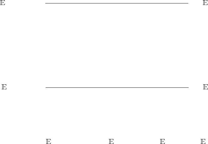
US borrowers face a choice between a mortgage with a higher interest and a lower upfront

closing cost or a mortgage with a lower interest rate and a higher upfront closing cost. I

illustrate this choice in Figure 1, which shows a series of options for rates and upfront closing

costs from a lender ratesheet. The ﬁrst column of the table in Figure 1 shows the choices of

interest rates that are available to a borrower, while the 15 Day, 30 Day, and 45 Day columns

show the corresponding upfront closing costs, quoted in percentages of the loan amount, that

borrowers would have to pay in order to receive the rate once the loan is originated within the

given lock period. A rate is “locked” when a lender commits to originating a mortgage with

the given terms within the stated lock period of, e.g., 15, 30, or 45 days. The quoted upfront

payment to the lender which vary by lock period are also called “points.” In particular,

Figure 1 shows how borrowers might choose a mortgage with a lower interest rate by paying

more points, or a mortgage with a higher interest rate by paying fewer (or, even, negative)

points.

Appendix Figure A.1 shows an example of how borrowers were shown a series of

rate and upfront closing cost choices from a price comparison website.

In this paper, I characterize mortgages with low or negative upfront closing costs as

mortgages with their price of mortgage origination added to the rate. To be more precise

about the deﬁnition of the price of mortgage origination added to the rate, focusing on the

setting where lenders are selling the mortgages they originate on the secondary market,

decompose lenders’ total origination revenue from making a loan as:

lender origination revenue

| {z }

price of mortgage origination

= upfront closing costs

| {z }

paid upfront

+ secondary marketing income(c)

| {z }

added into rate

(1)

where secondary marketing income(c) refers to the net income lenders derive from selling

a loan with interest rate c on the secondary market. The secondary marketing income can

be alternatively described as the premium of the mortgage relative to par. Mortgages with

higher interest rates tend to be more valuable on the secondary market and that originating

a mortgage with a high enough interest rate generates positive secondary marketing income.

To illustrate what the secondary marketing income as a function of interest rates might look

like on a given day, Figure A.2 plots the secondary market value of mortgages based on MBS

TBA prices as a percentage of the loan amount at various interest rates on January 2, 2014.

The TBA market is a highly liquid market where most MBS are traded, and is described in

Negative points are possible to cover the other upfront closing costs borrowers may have to pay, such as

transfer taxes and application fees.

Or, equivalently, where lenders are evaluating the value of their portfolio based on their potential sec-

ondary market value.

more detail in Vickery and Wright (2013).

3 Data

For my loan-level analyses, I use a combination of three data sets. The ﬁrst data set is the

2013–2019 data from Optimal Blue on rate locks. Optimal Blue is a rate-locking platform

used by lenders constituting about 40% of all U.S. mortgage originations. Mortgage lenders

use rate-locking platforms such as Optimal Blue to assist their loan originators and mortgage

brokers in identifying options for rate and upfront closing costs for their clients. It contains

information about interest rates, points paid or received by the borrower, and time of the

lock. Second, I use the 2013–2021 CRISM (Equifax Credit Risk Insight Servicing McDash

Database) data, which is an anonymous credit ﬁle match from Equifax consumer credit

database to Black Knight’s McDash loan-level mortgage data set. It contains information

on loan performance and a time-varying borrower characteristic in terms of their Equifax

Risk Score. The CRISM data also allows me to classify prepayments as moves or reﬁnances.

It has been frequently used to study borrower reﬁnancing behavior.

Third, I use the 2013–

2019 Home Mortgage Disclosure Act (HMDA) data to capture borrower demographics.

For my main empirical analysis, I construct a match of these data sets, leading to 2013–

2021 Optimal Blue-HMDA-CRISM match. I present some summary statistics of this 2013–

2021 Optimal Blue-HMDA-CRISM match in Table 1. I focus on 30-year, conforming, ﬁxed-

rate mortgages for my study due to their status as the most commonly chosen form of

mortgage contract in the US.

Further details of the matching procedure as well as additional

summary statistics can be found in the Appendix A.2.1 and A.2.

I follow the procedure of Lambie-Hanson and Reid (2018) and Gerardi, Willen, and Zhang (2021) to

identify moving by classifying a prepayment as a move if the borrower’s address changed within a 6-month

window surrounding the prepayment date.

See, e.g., Beraja et al. (2018), Lambie-Hanson and Reid (2018), Di Maggio, Kermani, and Palmer (2020),

Cunningham, Gerardi, and Shen (2021), Abel and Fuster (2021), and Gerardi, Willen, and Zhang (2021).

Complex mortgage contracts used to be more common before the ﬁnancial crisis, but have largely

vanished by the start of my sample period (Amromin, Huang, Sialm, and Zhong, 2018).

Finally, I obtain actual data on the rate and upfront closing cost menus from LoanSifter.

Summary statistics and more detailed descriptions of the LoanSifter data are shown in

Appendix A.2.3. I show that the rate and upfront closing cost trade-oﬀ from LoanSifter on

average closely matches the rate and secondary marketing income relationship as implied by

MBS TBA prices from Morgan Markets in Appendix A.3.

4 Motivating facts

In this section, I present some stylized facts that motivate my model. First, I show that bor-

rowers have heterogeneous reﬁnancing tendencies in Section 4.1. Second, I explore evidence

on the selection of borrowers with diﬀerent prepayment tendencies into upfront closing cost

choices in Section 4.2.

4.1 Heterogeneous reﬁnancing tendencies

It is well-known that some borrowers are slow to reﬁnance, while others are more quick to

reﬁnance when interest rates fall.

This is also true in my Optimal Blue-HMDA-CRISM

sample. In particular, Figure 2 plots the Kaplan-Meier survival hazards of prepayment

following months where the interest rate incentive for reﬁnancing, here deﬁned as the decrease

in the 30-year Freddie Mac survey rate, is greater than 1.2%, which is larger than the optimal

reﬁnancing threshold in typical calibrations of both the Agarwal, Driscoll, and Laibson (2013)

model and my model as presented in Section 5.

Speciﬁcally, the Kaplan-Meier estimates are calculated as follows. Let the number of

terminations due to prepayment at time t be p

, and the number of loans remaining at time

t be n

, where t is monthly. Then, the Kaplan-Meier hazard function is:

(t) =

. The

Kaplan-Meier survival function is then the cumulative eﬀect of the Kaplan-Meier hazard

These two data sets have also been used in Fuster, Lo, and Willen (2017) to study the time-varying price

of mortgage intermediation.

See, e.g., Archer and Ling (1993), McConnell and Singh (1994), Stanton (1995), Agarwal, Rosen, and

Yao (2016), Keys, Pope, and Pope (2016), Johnson, Meier, and Toubia (2018), and Andersen et al. (2018).

function, or

(t) =





Figure 2 shows the results. In particular, more than half of mortgages are not prepaid

after 10 months of a relatively high reﬁnancing incentive. While this could be due to supply-

side constraints, it also shows that the same pattern holds among a group of borrowers who

maintained an Equifax Risk Score of greater than or equal to 700 and an LTV of less than or

equal to 80% throughout the sample and are hence unlikely to be unable to reﬁnance due to

unemployment, eligibility, or cash ﬂow constraints. Even among this group of borrowers, I

ﬁnd that more half are not prepaid after 10 months of a relatively high reﬁnancing incentive.

4.2 Selection in choices of upfront closing costs

Second, I examine borrower choices of upfront closing costs in my Optimal Blue-HMDA-

CRISM data, paying particular attention to selection by borrower type. If borrowers all

know their prepayment types and choose upfront closing costs solely based on their expected

prepayment propensities, then there would be no cross-subsidization between borrowers de-

spite heterogeneity in prepayment propensities. The choice of upfront closing costs would

serve as a screening device that separates borrowers by type, as described in the models of

Brueckner (1994), LeRoy (1996), and Stanton and Wallace (2003). While I ﬁnd some selec-

tion in the data, I also ﬁnd evidence of within-choice heterogeneity in ex-post prepayment

and reﬁnancing behavior, which leaves room for cross-subsidization.

In this section, I measure borrower upfront closing costs in terms of “points,” where each

point is customarily one percent of the loan amount used to reduce the interest rate. Upfront

closing costs consist of points plus an application fee. Negative points, also called “lender

credit,” that reduce the total upfront closing costs paid are also possible. The reason I use

points rather than upfront closing costs in this analysis is that, unlike the 2018–2019 Optimal

Blue-HMDA data used to analyze upfront closing cost choices in Appendix Section A.4, the

2013–2021 Optimal Blue-HMDA-CRISM data contains only information on points and not

any other application fees the lender may charge. To the extent that these application fees

are constant within lender and loan type, my lender by county by year ﬁxed eﬀects within the

sample of 30-year, ﬁxed rate mortgages alleviates the eﬀects of the potential measurement

error.

First, I examine the extent to which borrowers with diﬀerent prepayment behavior choose

diﬀerent levels of upfront closing costs measured in terms of points. Figure 3 plots the distri-

bution of borrower choices of points by their eventual reﬁnancing or prepayment behavior.

I deﬁne a non-reﬁnancing borrower as one who did not reﬁnance or otherwise prepay within

ﬁve years despite facing a Freddie Mac Survey Rate decrease of at least 1.2%. As the ﬁgure

shows, although non-reﬁnancing borrowers on average pay more points, and borrowers who

prepay within ﬁve years on average pay fewer points, the diﬀerence is small in terms of the

overall distribution.

To make sure that the result of Figure 3 holds even after controlling for underwriting

variables, I run an OLS regression of the number of points paid with (1) an indicator function

for whether the borrower is a non-reﬁnancing borrower, and (2) an indicator function for

whether the borrower prepaid within ﬁve years. Results are shown in Table A.3. Indeed,

while I ﬁnd a statistically signiﬁcant positive correlation between non-reﬁnancing borrowers

and their payment of points, and a statistically signiﬁcant negative correlation between

borrowers who prepay within ﬁve years and their choices of points, the magnitude of the

diﬀerence in points paid is small at no more than 13 basis points. This analysis suggests

that most of the heterogeneity between borrower prepayment behavior remains conditional

on choices of upfront closing costs.

Next, I present regression estimates of how borrower choices of points correlate with their

prepayment behavior with choices of points and prepayment as the dependent variable. The

regressions are of the form:

i,t

= βX

+ γZ

+ ξ

i,t

×c

i,t

×t

+ 

i,t

(2)

where as before X

is a set of demographic and credit utilization variables including race

(Black and Hispanic), gender (male and female), credit card revolver status, and quartiles

of education; Z

is a set of underwriting variables including categories of credit scores at

origination, LTV, DTI, and log loan amount; ξ

i,t

×c

i,t

×t

is the lender by county by year ﬁxed

eﬀects. I run three regressions of this form with the indicator variable

i,t

being equal to the

amount of points paid, whether the mortgage was prepaid within ﬁve years, and whether

the mortgage was originated by a borrower who failed to reﬁnance despite facing a greater

than or equal to 1.2% reﬁnancing rate incentive.

Results are shown in Table 3. First, in terms of points, I ﬁnd that borrowers with a larger

loan amount pay more points, and that the correlation is small in terms of other borrower

characteristics. The correlation between point choices and predicted prepayment behavior is

also weak. For example, Black and Hispanic borrowers are signiﬁcantly less likely to prepay

their mortgage and more likely to be a non-reﬁnancing borrower, but their choices of points

are not statistically signiﬁcantly diﬀerent from zero compared to the other borrowers.

Another way to examine selection is to look at how borrower choices of points relate to

their moving and reﬁnancing behavior. Points do predict moving and prepayment behavior

in a statistically signiﬁcant manner, which is indicative of some selection being important

in this market. To do so, I run the the linear probability model on an indicator variable for

moving or reﬁnancing:

i,t

(move/reﬁ) =

j=1

(ψ

= j) + γZ

+ ξ

i,t

×c

i,t

×t

+ 

i,t

(3)

where

i,t

(move/reﬁ) is an indicator variable that is equal to either moving or reﬁnancing; β

are a set of coeﬃcients on categories of points choices as represented by the indicator function

(ψ

= j), and Z

is a set of controls including the call option value of reﬁnancing from Deng,

Bhutta and Hizmo (2019) ﬁnds that minority borrowers tend to pay fewer points. The discrepancy in

results can be explained by the fact that we focus on conforming mortgages rather than FHA mortgages

used in Bhutta and Hizmo (2019), and is explored in more detail in Willen and Zhang (2023).

Quigley, and Van Order (2000), the spread of the mortgage interest rate at origination to

the Freddie Mac Primary Market Survey Rate (spread at origination, or SATO) as well as

its square, and the standard set of loan amount, credit score at origination (credit score),

loan-to-value ratio (LTV), and debt-to-income ratio (DTI) controls. In particular, the call

option value of reﬁnancing is deﬁned as:

Call Option

i,k

i,m

− V

i,r

i,m

(4)

where

i,m

T M

−k

s=1

(1 + m

)

(5)

i,r

T M

−k

s=1

(1 + c

)

(6)

and c

is borrower i’s mortgage rate at origination, T M

is the mortgage term, k

is the

number of months already past, m

is the Freddie Mac Primary Market Survey Rate, and

is the size of the current mortgage payment. The Call Option variable represents the

potential interest rate savings from reﬁnancing, which is positively correlated with reﬁnancing

behavior. Finally, ξ

i,t

×c

i,t

×t

represents lender by county by year ﬁxed eﬀects, and 

i,t

is the

error term.

Figure 4 present the results. In particular, Figure 4a plots the predicted probabilities of

moving by categories of points paid in intervals of width 1. It shows that, all else equal,

the borrowers’ moving hazard is decreasing in the amount of points that they pay, which is

consistent with a selection story. Figure 4b shows the same pattern but for reﬁnancing.

Table 2 shows the regression coeﬃcients that underlie these results. The regression

coeﬃcients show a negative, monotone, and statistically signiﬁcant relationship between

the level of points paid and moving and reﬁnancing probabilities. In terms of additional

covariates, the Call Option, spread at origination SATO, and log of the loan amount are

positively correlated with moving and reﬁnancing.

The earlier analysis has focused on the diﬀerences between upfront closing cost choices

among borrowers. A question remains about the level of upfront closing cost choices, which

determines the extent to which borrowers pay their price of origination via the interest rate

or upfront, and how much of the price of origination may be susceptible to cross-subsidization

by borrower reﬁnancing tendencies. I show that almost all borrowers pay for most of their

mortgage closing costs through a higher interest rate on their mortgage relative to mortgage-

backed securities yields, rather than upfront in Appendix Section A.4.

Overall, my motivating facts imply that a model of cross-subsidization by prepayment

type has to take into account both the within-choice heterogeneity in prepayment behavior as

well as the selection of borrowers into point choices by their ex ante prepayment expectation.

My model accomplishes both of these tasks. In particular, by estimating a distribution of ex

ante moving and reﬁnancing types and how they correlate through borrower choices of points,

it simultaneously incorporates both selection and within-choice borrower heterogeneity.

5 Model

The motivating facts in Section 4 show that the existence of signiﬁcant reﬁnancing inertia in

the US mortgage market as well as selection of mortgage contracts by borrower prepayment

types. Because borrower reﬁnancing behavior is an important determinant of mortgage inter-

est rates, an equilibrium model that incorporates the supply side (ie. mortgage interest rate)

response to heterogeneity in reﬁnancing behavior is needed to get at the welfare questions.

I build such an equilibrium of mortgage choice that captures the heterogeneity in borrower

reﬁnancing behavior and allows me to assess its welfare implications in dollar terms.

On the demand side, following the state-of-the-art from Andersen et al. (2018), I estimate

a distribution of borrower reﬁnancing costs with two components: a ﬁxed reﬁnancing hassle

cost and a time varying ability to reﬁnance. In addition, borrowers diﬀer by their moving

probabilities and discount factors. These decisions are then embedded in a workhorse life-

cycle model of mortgage choice from Campbell and Cocco (2015) and Chen, Michaux, and

Roussanov (2020). A competitive supply side pins down mortgage interest rates at various

levels of upfront closing costs and closes the model.

Calibration of the model shows evidence of large cross-subsidization of low upfront clos-

ing cost mortgages from slow to reﬁnance borrowers. In addition, the fully estimated model

allows me to measure the welfare implications of heterogeneity in borrower reﬁnancing ten-

dencies in equilibrium.

5.1 Setup

5.1.1 Demand side

On the demand side, households maximize non-housing consumption with time-separable

utility with bequest motive for terminal wealth taking housing choice as exogenous:

max

t=1

t−1

)

1−γ

1 − γ

+ β

1−γ

i,T +1

1 − γ

, (7)

where T is the terminal age, β

the time discount factor, C

the non-durable consumption,

the coeﬃcient of relative risk aversion, and W

i,T +1

the real terminal wealth.

In terms of exogenous state transitions, I assume that the risk-free rate r

follows the

model of Cox, Ingersoll, and Ross (1985), which has a natural zero lower bound. I take

inﬂation π = 1.68% as a constant equal to the average in my sample.

Real (log)labor

income L

, house price H

, and changes in the mortgage interest rate at an average level of

upfront closing costs ∆¯c

are modelled as a vector auto-regression (VAR) with the risk-free

rate r

as an exogenous covariate, the details of which are described in Appendix A.6.1.

Finally, moving is treated as an exogenous mortgage reﬁnance at an average level of upfront

Inﬂation expectations were stable over my sample period, and a constant term for inﬂation allows me

to easily convert the nominal mortgage payment from the amortization table to real terms.

closing costs.

Mortgage payments follow a standard 30 year amortization schedule. In particular, the

real mortgage payment under constant inﬂation is P

(1+π)

/12(1+c

/12)

(1+c

/12)

−1

. Note that

the amortization is based on the current rate rather than the full history of rates, which

increases the computational tractability of the model. I add a correction for the diﬀerence in

amortization as an additional upfront payment to be made by the borrower during reﬁnancing

so as to be more numerically correct, but the error resulting from this issue is likely to be

small for minor diﬀerences in rates.

In each period, households make a decision of whether to reﬁnance along with a con-

sumption and savings decision. In doing so, they face ﬁnancial constraints in the sense that

their savings S

≥ 0. They make a real mortgage payment P

and earn interest r

savings minus inﬂation π

, and so in non-reﬁnancing periods their non-durable consumption

in real terms can be written as:

= exp(L

) − P

+ (r

1,t−1

− π

it−1

− ∆S

(8)

Where ∆S

= S

− S

it−1

is the change in the borrower’s savings. In order to reﬁnance,

borrowers need to pay a cost ˜κ

. I model the borrowers’ reﬁnancing cost ˜κ

as:

˜κ











∞, with probability 1 − p

, with probability p

(9)

where p

is the probability that a borrower is able to reﬁnance in a particular time period.

The inclusion of time- and state-varying reﬁnancing costs is necessary to ﬁt the data where

borrowers do not immediately reﬁnance when facing their cut-oﬀ, as described in Andersen

et al. (2018) which uses a similar setup for capturing reﬁnancing costs.

Furthermore, I require that the reﬁnance must leave the borrower a loan-to-value (LTV)

ratio of at most 95%, which is required by Freddie Mac

and captures the constraints to

reﬁnancing in periods of house price decline as described in Hurst, Keys, Seru, and Vavra

(2016).

The full value function V

, S

i,t−1

, ¯c

, r

1,t−1

, H

i,t−1

, L

) is a function of the state vari-

ables interest rate on the mortgage c

, last period savings S

i,t−1

, the current market interest

rate ¯c

, last period’s risk-free rate r

1,t−1

, house price H

, lagged house prices H

i,t−1

, labor

income L

. Of these variables, c

, S

are endogencous in that they are inﬂuenced by the deci-

sion to reﬁnance and borrower’s consumption decision, while the other states are exogenous.

In what follows I write the value function

, S

) = V

, S

, ¯c

, r

1,t−1

, H

i,t−1

, L

)

as a function of the endogenous variables only for brevity.

When ﬁrst getting a mortgage, borrowers make a choice of mortgage interest rate c along

with their associated upfront closing cost ψ

ﬁrst period:

= max

∆S

(exp(L

) − (˜κ

+ ψ

(c)M) − ∆S

)

1−γ

1 − γ

+ β

(c, S

) (10)

In the following periods, borrowers make a mortgage payment P

). And in periods

where the borrower is able to reﬁnance, their utility can be written as the maximum of what

can be obtained by reﬁnancing and not reﬁnancing:

= max











max

∆S

(exp(L

)−P

)+(r

1,t−1

−π

it−1

−∆S

)

1−γ

+ β

i,t+1

, S

)

max

∆S

(exp(L

)−P

)−(˜κ

+ψ

(c)M)+(r

1,t−1

−π

it−1

−∆S

)

1−γ

+ β

i,t+1

(c, S

)

(11)

where the ﬁrst line of Equation (11) corresponds to the borrower’s utility from not reﬁnancing

and continuing to get the interest rate c

, while the second line corresponds to the borrower’s

Freddie Mac’s requirements for reﬁnancing are described in https://sf.freddiemac.com/general/maximum-

ltv-tltv-htltv-ratio-requirements-for-conforming-and-super-conforming-mortgages. Fannie Mae has a slightly

looser LTV requirement of at most 97%: https://singlefamily.fanniemae.com/media/20786/display.

utility from reﬁnancing to the rate c which aﬀects the upfront closing cost they pay ψ

(c).

Similarly, the borrower’s utility given that they are not able to reﬁnance is:

= max

∆S

(exp(L

) − P

− (r

− π

i,t−1

− ∆S

)

1−γ

1 − γ

+ β

i,t+1

, S

). (12)

Finally, I model moving as an exogenous costless reﬁnance to the new mortgage with an

interest rate ¯c

that is associated with an average level of closing costs, which occurs with

probability p

for borrower i. Therefore, the borrower’s utility upon moving is:

= max

∆S

(exp(L

) − P

− (r

− π

i,t−1

− ∆S

)

1−γ

1 − γ

+ β

i,t+1

(¯c

, S

). (13)

Combined, the value function of the borrower can be written as:

= (1 − p

)(p

+ (1 − p

)

) + p

. (14)

5.1.2 Supply side

A supply side to the model is needed compute mortgage premia with counterfactual mortgage

contract designs. I assume that the supply side is perfectly competitive and that lenders

set the rate and upfront closing cost/points trade-oﬀ based on the MBS value of mortgages.

That is, in equilibrium the relationship between the upfront closing costs paid as a fraction

of the loan amount ψ

for borrower i at time t and the mortgage interest rate c is pinned

down by a zero proﬁt condition:

= ψ

M + φ

(c)M − ¯m

− m

(M) = 0 (15)

where π

is lender proﬁt from a originating loan to borrower i at time t, φ

premium of the mortgage as a percent of the loan amount at the time of origination, and ¯m

is average marginal cost incurred by the lender for originating the loan, and m

(M) is the

borrower and loan amount speciﬁc marginal cost incurred by the lender for originating the

loan. Assuming that the marginal cost of loan origination ¯m

+ m

(M) does not vary by the

borrower’s choice of points, we have by re-arranging:

¯m

+ m

(M)

− φ

(c). (16)

So that, all else equal, a mortgage with a higher interest rate c and MBS value φ

(c)

would require fewer upfront points ψ

. In particular, my model implies that the MBS value

of mortgages with a higher interest rate will be passed-through to borrowers in terms of

lower upfront closing costs. This pass-through implication is approximately true in reality,

as I show in Figure A.3.

The zero proﬁt condition in Equation (16) requires an estimate of MBS prices φ

(c).

These prices incorporate heterogeneous borrower reﬁnancing behavior in the current world,

but not in counterfactuals without cross-subsidization between borrower reﬁnancing types.

Estimation of these counterfactual prices is therefore key to establishing the interest rate

eﬀect of heterogeneous borrower reﬁnancing behavior.

I estimate the MBS value of mortgages φ

where the cashﬂows from MBS are assumed to be discounted using the risk-free rate r

plus an option-adjusted spread (OAS) term that compensates for the the liquidity and

prepayment risk. The OAS has been used and evaluated as a proxy for expected MBS returns

in Gabaix, Krishnamurthy, and Vigneron (2007), Song and Zhu (2018), and Boyarchenko,

Fuster, and Lucca (2019), and Diep, Eisfeldt, and Richardson (2021).

Under this setup,

the MBS value of mortgages may be written as:

(c)M = E

t+T

[(1 − p

] − M (17)

Another method of valuing MBS is via multivariate density estimation, as in Boudoukh, Whitelaw,

Richardson, and Stanton (1997), but that does not allow me to get counterfactual prices under alternative

prepayment behavior or with alternative mortgage contract designs.

where p

is the prepayment probability of the borrower at time t

, q

−1

j=t

(1 −p

) is the

remaining proportion of borrowers who have not prepaid, B

is the remaining principal the

lender gets when a borrower prepays, the lender gets remaining principal B

, and P

the regular mortgage payment. The discount factor is based on the cumulative risk-free rate

in period j, r

, plus an estimated OAS term that compensates for liquidity and prepayment

risk:

j=t

(1 + r

+ OAS)

. (18)

Based on Equations 17 and (18), an estimate of the OAS combined with borrower reﬁ-

nancing behavior allows me to arrive at counterfactual MBS prices. To estimate the OAS,

I use actual MBS prices combined with an empirical prepayment hazard function ˆp

and

its implied empirical cumulative remaining balance ˆq

−1

j=t

(1 − ˆp

). Details of the OAS

estimation is shown in Appendix A.6.2.

The no cross-subsidization counterfactual, or the equilibrium without pooling of borrower

prepayment types, is computed by: (i) computing the required lender payoﬀ in each state

as implied by the estimated OAS and ˆp, conditional on ¯c

and r

as state variables, and

then (ii) ﬁnding the rate-point trade-oﬀ in separating equilibrium in each period via joint

iteration, where each period represents one quarter of calendar time. The joint iteration is

conducted as follows. In the last period, borrowers cannot reﬁnance. In the second to last

period, the lender creates a rate-and-upfront closing costs schedule based on the borrower’s

expected behavior in the last period and the required lender payoﬀ, and then the borrower

makes a reﬁnancing decision conditional on their state and the lender’s schedule, and so on.

Combined with the demand side, my model can be viewed as an equilibrium model of

mortgage premia, in line with Campbell and Cocco (2015) and Campbell, Clara, and Cocco

(2021), but with the addition of heterogenous borrower reﬁnancing costs and endogenous

upfront closing costs. A key assumption in these models is the perfectly competitive supply

side. If the supply side were not perfectly competitive as is assumed here, my pricing results

would still hold if lenders charged a constant markup across loans (i.e. so that constant

revenue per loan in the counterfactual still holds).

5.2 Cross-subsidization by upfront closing cost choice: a calibra-

tion

Using the model, I illustrate the cross-subsidization of low upfront closing cost mortgages

from the perspective of a quick to reﬁnance borrower through a calibration. All of the

analysis in this section is conducted for a calibrated borrower with parameters described in

Table 4, where β, M, p

are the median of the estimates from Section 6, and p

= 1, κ

= 200

are chosen to represent the behavior of an optimally reﬁnancing borrower who is always able

to reﬁnance with a hassle cost of $200.

Figure 5 illustrates this pricing impact of cross-subsidization by plotting the implied

interest rates from the joint iteration of borrower and lender values in the dashed line. The

market rate and upfront closing cost rate-oﬀ as implied by the model is shown in the solid

line, and the empirical rate and upfront closing cost trade-oﬀ is presented in the dotted line.

The close match between the two suggests that the supply side of the model, which is the

previously described OAS model of MBS valuation, matches the average empirical rate and

upfront closing cost well.

As Figure 5 shows, the interest rate trade-oﬀ is higher, and steeper, for the calibrated

quick to reﬁnance borrower in the no cross-subsidization counterfactual. This suggests that

the market interest rate for low upfront closing cost mortgages is especially lower than in

the no cross-subsidization case due to the presence of slow to reﬁnance borrowers. In terms

of numbers, I ﬁnd that a mortgage with a one percent upfront closing cost would carry a

0.97% higher interest rate in the no cross-subsidization case relative to the existing market

equilibrium, whereas the diﬀerence is only 0.21% for a mortgage with a four percent upfront

closing cost.

Figure 6 presents the welfare implications of this calibration for the borrower, lender, and

society. The calibrated quick to reﬁnance borrower beneﬁts from cross-subsidization, and

would have to be paid 2.4% of the loan amount in liquid assets in the no cross-subsidization

counterfactual in order to be indiﬀerent from the current world. The lender, on the other

land, loses 5.5% of the loan amount in proﬁt in the current world relative to the no cross-

subsidization counterfactual. Since the lender loses more than the borrower gains, cross-

subsidization led to a social loss of 3.0% of the loan amount. This social loss comes from the

excessive reﬁnancing that the quick to reﬁnance borrowers undertake at the expense of the

slow to reﬁnance borrowers in the market, which in the calibration is 1.74 times as frequent

in expectation relative to the no cross-subsidization counterfactual.

6 Estimation

To estimate the model, I allow p

, κ

, β

, p

, M

to vary by individual, where p

is the prob-

ability that an individual is available to reﬁnance in a particular time period, κ

is the

individual’s reﬁnancing hassle cost when they do reﬁnance, β

is the discount factor, p

the individual’s moving probability, and M

is the individual’s mortgage size. I ﬁx the coef-

ﬁcient of risk aversion γ = 2, liquid savings at origination to $50k, and a bequest motive of

b = 200 in accordance with Campbell and Cocco (2015). To maintain comparability to the

TBA market, I further restrict my analysis to 30 year purchase mortgages with a balance

above $150k, FICO above 680, and LTV below 85% following Fusari, Li, Liu, and Song

(2020).

I ﬁrst present the identiﬁcation argument in Section 6.1, then estimation procedure in

Section 6.2, then results in Section 6.3, some calibration based on my estimates in Section 5.2,

and ﬁnally the implications of my estimates for transfers and welfare in Section 6.4.

6.1 Identiﬁcation

Of the unknown parameters, the distribution of M

is observed. I discuss the identiﬁcation

for the distribution of p

, κ

, β

, p

as follows. First, the time-varying ability to reﬁnance

and hassle costs κ

are separately identiﬁed from borrower responses to the time series

movement of the interest rate incentive. More speciﬁcally, if the only heterogeneity in bor-

rower reﬁnancing behavior were due to hassle costs, borrowers would reﬁnance immediately

when their reﬁnancing cutoﬀ is reached. This is rejected in the data as many borrowers wait

long after the interest rate has fallen to their eventual reﬁnancing rate, suggesting that a

time-varying reﬁnancing cost is at play. This line of reasoning is also used in Andersen et al.

(2020).

Of the other parameters, ex ante moving probabilities p

are identiﬁed from the inter-

action between the interest rate incentive and borrower reﬁnancing behavior. In particular,

borrowers who do not reﬁnance when faced with a large interest rate incentive are more

likely to subsequently move. This suggests that moving is not just an ex post shock and that

there is heterogeneity in moving expectations ex ante. Finally, conditional on reﬁnancing

and moving probabilities, discount factors β

are identiﬁed from borrower choices of upfront

closing costs. In general, because upfront closing costs involve an initial outlay, they are

more attractive to borrowers with a higher discount factor. The choices of borrowers who

choose low upfront closing cost mortgages despite being unlikely to reﬁnance or move are

rationalized with a lower discount factor.

6.2 Parametrization

I estimate the distribution of the borrower types using mortgage performance data. More

speciﬁcally, I use a Logit-Normal distribution

to model p

, β

, p

, a Log-Normal distribution

to model κ

, and allow p

, β

to be correlated via a coeﬃcient ρ. The precise parametrization

The Logit-Normal distribution is the distribution generated by Y =

exp(X)

1+exp(X)

with a normally distributed

X. This formulation allows me to model observations that are between zero and one, as well as correlations

between them, in closed form.

is as follows:













∼ Logit







MultivariateNormal













(b, h)













ρσ



















(19)

∼ Logit(Normal(µ

(b, h), σ

)) (20)

∼ LogNormal(µ

(b, h), σ

) (21)

where µ

(b, h), µ

(b, h) can depend on a Black and Hispanic dummy represented

by b and h, respectively. This gives me 15 parameters:

θ = (µ

(0, 0), µ

(1, 0), µ

(0, 1), σ

, µ

(0, 0), µ

(1, 0),

(0, 1), σ

, µ

(0, 0), µ

(1, 0), µ

(0, 1), σ

, µ

, σ

, ρ)

to estimate. I focus on the correlation ρ between a borrower’s probability of being able

to reﬁnance and their discount factor because variation in the distribution of κ is small.

Intuitively, this is because when borrowers do reﬁnance, they tend to do so for relatively

low interest rate savings (ie. in the range of 1%), which would not be reconcilable with

a high reﬁnancing hassle cost κ. Therefore, time-varying ability to reﬁnance appears more

important in the data, and I also estimate its correlation with the borrowers’ discount factors.

In the data, I observe borrowers’ prepayment decisions which combines moving and reﬁ-

nancing.

I construct the likelihood based on prepayment decisions, which implicitly treats

all non-model implied reﬁnancing as a move. Therefore, the moving probability p

in my

model captures all exogenous prepayment. The likelihood function for a prepayment decision

for loan j at time t given a set of parameters x

= {p

, κ

, β

, p

, M

} is then:

) = (1 − y

)

1−p

)

. (22)

I also separately observe moving and reﬁnancing decisions for a subset of prepayments.

Furthermore, at time t = 0, the likelihood of observing the borrower with ’s choice of

upfront closing costs ψ

that is equal to the optimal choice implied by the model of ψ

∗

) = (ψ

= ψ

∗

)). (23)

To estimate the model, I simulate individuals with a grid for x

= {p

, κ

, β

, p

, M

}

based on a set of parameters θ, with x

∼ F(θ) where F(θ) is the distribution of types from

Equations (19) to (21). I then get their model implied optimal point choices (ψ

∗

), in whole

numbers from -2 to 2) and time-varying prepayment (i.e., reﬁnancing and moving) decisions

for each loan-time observation p

), and search for the set of parameters that maximizes

the likelihood of the data following the standard maximum likelihood formulation:

L ∝

log





nsim

i=1

)

t=1

j,t

)





, x

∼ F(θ), (24)

where nsim = 2000 is the number of simulations used to compute the likelihood function.

6.3 Results

In this section I present my estimates for the distribution of borrower types in the population.

The parameters and their standard errors are shown in Appendix Table 5, and I plot their

distributions in the rest of this section.

Figure 7 presents the estimates on the distribution of reﬁnancing types in the population.

In the left panel in Figure 7a, results show that most borrowers have a low probability of

being able to reﬁnance in a particular month, with some variance. Mean able-to-reﬁnance

probability is 6.0% monthly, or 52% annualized. This is consistent with my stylized fact in

Section 4.1 showing that around half of all borrowers fail to reﬁnance following ten months

of a relatively high reﬁnancing incentive. In the right panel in Figure 7b, the results show

Since I only observe points and not application fees prior to 2018, I assume a real application fee of

$2000 following Agarwal, Driscoll, and Laibson (2013).

that the implied hassle cost of reﬁnancing for most borrowers is low. Taken together, the

results suggest that most of the inaction in reﬁnancing is due to a Calvo-style time-varying

ability to reﬁnance rather than hassle costs. The identiﬁcation in the data is that borrowers

who eventually reﬁnance tend to do so at relatively low interest rate savings (for example,

at around 1%), which implies a low hassle cost for reﬁnancing for most borrowers despite a

time-varying inability to do so.

Figure 8 presents my estimates for borrower discount factors and their correlation with

their time-varying ability to reﬁnance. Figure 8a plots the distribution of discount factors,

which is above 0.9 for most borrowers, but there is a small group of borrowers with discount

factors closer to 0.0. The discount factors are identiﬁed from borrower choices of upfront

closing costs, and the existence of many borrowers with low reﬁnancing/moving probabilities

but nevertheless get higher interest rate, lower closing cost mortgages is rationalized in the

model via borrower myopia. Figure 8b shows a strong correlation between the likelihood of

being able to reﬁnance and the discount factor. It is a scatterplot drawn from the multivariate

Logit-Normal distribution of Equation (19). It shows that many borrowers with a probability

of being able to reﬁnance in a particular month of less than 5% also have a discount factor

signiﬁcantly lower than 0.9. On the other hand, borrowers with a probability of being able

to reﬁnance in a particular month of greater than or equal to 5% tend to have a discount

factor above 0.95.

Finally, Figure 9 presents my estimates of the distribution of moving probabilities by

borrower. Ex ante expectations of probabilities are identiﬁed from the joint interaction

of reﬁnancing hazards and the interest rate incentive to reﬁnance. As Figure 9 shows,

annualized moving probabilities are centered around 11% per year, with some groups of

borrowers having a lower moving probability. Appendix Figure A.16 plots these distributions

by the racial group of the borrower.

6.4 Implications for transfers and welfare

In this section I use my empirical estimates to examine the deviation of borrower behavior

from the perfect information benchmark. Doing so allows me to reveal the transfers and

eﬃciency consequences of heterogeneity in borrower reﬁnancing behavior when interacted

with the ﬁnancial contract design of adding closing costs to the rate of the mortgage.

Figure 10 plots the diﬀerences in utility in the actual world versus the no perfect informa-

tion, no cross-subsidization benchmark. I ﬁnd an average welfare loss of $445 per mortgage,

most of it borne by borrowers with a probability of being able to reﬁnance of less than

5%. Given that there are around 8 million new mortgages being originated per year, the

welfare loss from the closing cost channel of cross subsidization is around $3.6 billion per

year. In addition, the average utility diﬀerence to the perfect information benchmark, in

absolute dollar value terms, is $1339/borrower, suggesting an average diﬀerence in utility of

1% of the loan amount from slow to reﬁnance borrowers to quick to reﬁnance borrowers.

By comparison, the diﬀerence in utility from comparing the benchmark quick to reﬁnance

borrower as calibrated in Section 5.2 to a non-reﬁnancing borrower that has p

= 0 but are

otherwise similar for a mortgage with zero upfront closing costs is 3.5% of the loan amount.

Figure 11 plots the welfare eﬀects of the cross-subsidization by racial group. The welfare

eﬀects are -$1776 per households for Black borrowers, -$1448 per households for Hispanic

borrowers, and -$366/borrower for other households. The welfare impact is negative for

all racial groups in part due to the deadweight loss generated by the cross-subsidization of

mortgage closing costs, but it is particularly strong for minorities.

To get at the excessive reﬁnancing incentives generated by the cross-subsidization of

mortgage closing costs, Figure 12 plots the diﬀerences in the expected number of reﬁnances

per new origination in the actual world versus the perfect information, no cross-subsidization

benchmark. I ﬁnd an average increase of 0.13 reﬁnances per new purchase origination. My

This diﬀerence in utility is approximated by doubling the average utility diﬀerence to the perfect infor-

mation benchmark, or $2678/borrower, and dividing by the average loan size of $252,000.

model implies an average number of reﬁnances per new purchase origination of 0.47. There-

fore, it implies that 27.5% of the total US mortgage reﬁnancing volume may be considered

excessive relative to the perfect information benchmark.

7 Counterfactuals

I conduct two counterfactual analyses. First, I consider an alternative mortgage contract

design where closing costs have to be added to the balance of the loan. The advantage

of this design is that it eliminates the cross-subsidization of mortgage closing costs: all

borrowers have to pay for their own price of mortgage origination. Second, I consider the

case of automatically reﬁnancing mortgages, which is a mortgage whose interest rate resets

downwards automatically to a lower rate when the market rates falls by more than 1%.

This contract has been discussed in Campbell (2006). In both of these cases, I compute

the updated borrower and lender value functions, and I re-estimate the equilibrium using

the same zero proﬁt condition on the supply side. To avoid complications with multiple

equilibria, I restrict myself to counterfactuals where upfront closing cost choices are ﬁxed.

7.1 Adding closing cost to balance

First, I consider the utility changes of borrowers when they add their closing cost to the

balance of the loan. That is, their new mortgage balance becomes M

= M(1 + c

(M)), and

their mortgage payment becomes:

) = M

/12(1 + c

/12)

(1 + c

/12)

− 1

. (25)

In periods where borrowers are able to reﬁnance, their utility can still be written as the

maximum of what can be obtained by reﬁnancing and not reﬁnancing, except that reﬁnancing

increases the balance of the loan from M to M

. Hence, M becomes an endogenous state

variable that we add to the model which aﬀects the size of the mortgage payment P

The expected utility in periods where borrowers are able to reﬁnance,

i,t

, is then:

i,t

= max











max

∆S

(exp(L

)−P

(M)−(r

1,t−1

−π

i,t−1

−∆S

)

1−γ

+ β

i,t+1

, S

, M), if no move/reﬁ

max

∆S

(exp(L

)−P

)−˜κ

−(r

1,t−1

−π

i,t−1

−∆S

)

1−γ

+ β

i,t+1

, S

, M

), if reﬁ

(26)

I simulate borrower utility and prepayment behavior under this counterfactual with bor-

rower utility when they are able to reﬁnance being described by Equation (26) instead of

Equation (11). I then obtain the implied aggregate borrower behavior and lender values

based on my estimated distribution of borrower types in Table 5, conditional on the paths of

interest rates as estimated in Section A.6.1. Finally, I decrease the initial mortgage interest

rate for all borrowers, holding ﬁxed their prepayment behavior, until the zero proﬁt condition

in Equation (16) is satisﬁed on average, which is an equilibrium eﬀect of this contract design

that increases in borrower utility.

Results are shown in Figure 13a, with a signiﬁcantly narrower range of utility diﬀerences

relative to the perfect information benchmark. When closing costs are added to the balance

of the mortgage, there are still gains from actively reﬁnancing relative to not reﬁnancing,

albeit less than in the current world. This reduces the cross-subsidization between borrower

types. In particular, the average utility diﬀerence to the perfect information benchmark, in

absolute dollar value terms, falls by around half from $1339/borrower in the current world to

$698/borrower in this counterfactual world. The same reduction in cross-subsidization can

be inferred from Figure 13b, which plots the mean utility diﬀerence to the perfect information

case, in dollar terms, by buckets of borrower reﬁnancing ability.

In terms of total welfare, I ﬁnd that on average consumer welfare relative to the perfect

information benchmark rises from -$446/borrower to $110/borrower. Not only is the negative

welfare impact of excessive reﬁnancing eliminated in this contract design, but there is also

a welfare gain due to the relaxation of ﬁnancial constraints as closing costs can be added

to the balance. In the current world, actively reﬁnancing borrowers can only pre-commit to

not undertaking costly reﬁnancing activity by paying more in upfront closing costs, which is

itself costly due to ﬁnancial constraints. Otherwise, they would have to take a higher initial

interest rate and reﬁnance more which carries administrative resource costs. The addition

of mortgage closing costs to the balance both eliminates the cross-subsidization of mortgage

closing costs and resolves this commitment problem. As a result, it is able to simulatenously

reduce transfers by borrowers with diﬀerent reﬁnancing tendencies and also increase total

welfare.

Appendix Figure A.17 plots the counterfactual change in utility by racial group under

the alternative contract design of adding all closing costs to the balance of the loan. All

racial groups gain from this counterfactual, with Black borrowers gaining on average $1566,

Hispanic borrowers gaining $1325, and other borrowers gaining $472. The average welfare

gain under this counterfactual is $556.

7.2 Making mortgages automatically reﬁnancing

Second, I consider a counterfactual where mortgages are automatically reﬁnancing and are

originated with zero upfront closing costs. In this case, I keep the same demand as in

Section 5 but automatically change the mortgage interest rate from c to r whenever c−r > 1

conditional on the paths of interest rates as estimated in Section A.6.1. Furthermore, I

eliminate the possibility of reﬁnancing as that is no longer relevant. Finally, I increase

the initial mortgage premia over the risk-free rate for all borrowers until the zero proﬁt

condition in Equation (16) is satisﬁed in the counterfactual, which is an equilibrium eﬀect

of this contract design that decreases borrower utility.

Results are shown in Figure 14. I terms of distribution, automatically reﬁnancing mort-

gages also feature lower average utility diﬀerence to the perfect information benchmark com-

pared to the current world. In particular, I ﬁnd that this statistic falls from $1339/mortgage

to $773/mortgage. Furthermore, the automatically reﬁnancing mortgages counterfactual fea-

ture a greater welfare improvement relative to the current world compared to adding closing

costs to the balance of the loan, at $1216/mortgage. This signiﬁcant improvement is due to

the resource cost savings of reﬁnancing, and is concentrated among the actively reﬁnancing

borrowers as shown in Figure 14b. Appendix Figure A.18 plots the counterfactual change

in utility by racial group under the alternative contract design of automatically reﬁnanc-

ing mortgages, showing that all racial groups would on average increase their utility in this

counterfactual.

Conceptually, there are two main channels through which automatically reﬁnancing mort-

gages can increase total welfare. First, they can eliminate the excessive reﬁnancing incentives

from the cross-subsidization of mortgage closing costs. Second, they also generate resource

savings by eliminating the administrative and hassle costs of reﬁnancing. To the extent that

automatically reﬁnancing mortgages present real resource savings to the economy and enable

a more eﬃcient pass-through of monetary policy not modelled here, it may be an attractive

contract design for policymakers to consider.

8 Conclusion

The broad lesson of my paper is that in markets for consumer ﬁnancial products, seemingly

small contractual details can have signiﬁcant equity and eﬃciency implications. I illustrate

this lesson quantitatively in the US mortgage market where borrowers typically choose to

ﬁnance their closing costs through the rate. I show that this contractual feature exacerbates

transfers between borrower reﬁnancing types while also generating deadweight losses through

incentivizing excessive origination. In terms of policy, my results suggest that two alternative

mortgage contract designs—(1) adding closing costs to the balance of the loan and (2) having

automatically reﬁnancing mortgages—can simultaneously reduce inequality in the market

and improve total consumer welfare.

References

Abel, Joshua, and Andreas Fuster. 2021. “How Do Mortgage Reﬁnances Aﬀect Debt, Default,

and Spending? Evidence from HARP.” American Economic Journal: Macroeconomics

13(2): 254–291.

Agarwal, Sumit, Itzhak Ben-David, and Vincent Yao. 2017. “Systematic Mistakes in the

Mortgage Market and Lack of Financial Sophistication.” Journal of Financial Economics

123(1): 42–58. ISSN 0304-405X.

Agarwal, Sumit, John C. Driscoll, and David I. Laibson. 2013. “Optimal Mortgage Reﬁnanc-

ing: A Closed-Form Solution.” Journal of Money, Credit and Banking 45(4): 591–622.

Agarwal, Sumit, Richard J. Rosen, and Vincent Yao. 2016. “Why Do Borrowers Make

Mortgage Reﬁnancing Mistakes?” Management Science 62(12): 3494–3509.

Ambokar, Sumedh, and Kian Samaee. 2019. “Inaction, Search Costs, and Market Power in

the US Mortgage Market.” Working Paper.

Amromin, Gene, Jennifer Huang, Clemens Sialm, and Edward Zhong. 2018. “Complex

Mortgages.” Review of Finance 22(6): 1975–2007.

Andersen, Steﬀen, John Y. Campbell, Kasper Meisner Nielsen, and Tarun Ramadorai. 2018.

“Sources of Inaction in Household Finance: Evidence from the Danish Mortgage Market.”

Working Paper.

Andersen, Steﬀen, John Y. Campbell, Kasper Meisner Nielsen, and Tarun Ramadorai. 2020.

“Sources of Inaction in Household Finance: Evidence from the Danish Mortgage Market.”

American Economic Review 110(10): 3184–3230. doi:10.1257/aer.20180865.

Archer, Wayne R., and David C. Ling. 1993. “Pricing Mortgage-Backed Securities: Integrat-

ing Optimal Call and Empirical Models of Prepayment.” Real Estate Economics 21(4):

373–404.

Bartlett, Robert, Adair Morse, Richard Stanton, and Nancy Wallace. 2019. “Consumer-

Lending Discrimination in the FinTech Era.” Working Paper.

Belgibayeva, Adiya, Teresa Bono, Philippe Bracke, Jo˜ao Cocco, and Tommaso Majer. 2020.

“When Discounted Rates End: The Cost of Taking Action in the Mortgage Market.” FCA

Occasional Paper No. 54.

Benetton, Matteo, Alessandro Gavazza, and Paolo Surico. 2020. “Inaction, Search Costs,

and Market Power in the US Mortgage Market.” Working Paper.

Beraja, Martin, Andreas Fuster, Erik Hurst, and Joseph Vavra. 2018. “Regional Heterogene-

ity and the Reﬁnancing Channel of Monetary Policy.” Quarterly Journal of Economics

134(1): 109–183.

Berger, David, Konstantin Milbradt, Fabrice Tourre, and Joe Vavra. 2023. “Reﬁnancing

Frictions, Mortgage Pricing and Redistribution.” Working Paper.

Bhutta, Neil, and Glenn B Canner. 2013. “Mortgage Market Conditions and Borrower

Outcomes: Evidence from the 2012 HMDA data and Matched HMDA-Credit Record

Data.” Federal Reserve Bulletin 99(4): 1–58.

Bhutta, Neil, and Aurel Hizmo. 2019. “Do Minorities Pay More for Mortgages?” Working

Paper.

Boudoukh, Jacob, Robert F Whitelaw, Matthew Richardson, and Richard Stanton. 1997.

“Pricing mortgage-backed securities in a multifactor interest rate environment: A multi-

variate density estimation approach.” The Review of Financial Studies 10(2): 405–446.

Boyarchenko, Nina, Andreas Fuster, and David O. Lucca. 2019. “Understanding Mortgage

Spreads.” Review of Financial Studies 32(10): 3799–3850.

Brueckner, Jan K. 1994. “Borrower Mobility, Adverse Selection, and Mortgage Points.”

Journal of Financial Intermediation 3(4): 416–441.

Campbell, John Y. 2006. “Household Finance, Presidential Address to the American Finance

Association.” Journal of Finance LXI(4): 1553–1604.

Campbell, John Y., Nuno Clara, and Jo˜ao F. Cocco. 2021. “Structuring Mortgages for

Macroeconomic Stability.” Journal of Finance 76: 2525–2576.

Campbell, John Y., and Joao F. Cocco. 2003. “Household Risk Management and Optimal

Mortgage Choice.” Quarterly Journal of Economics 118(4): 1449–1494.

Campbell, John Y., and Joao F. Cocco. 2015. “A Model of Mortgage Default.” Journal of

Finance 70(4): 1495–1554.

Chari, V. V., and Ravi Jagannathan. 1989. “Adverse Selection in a Model of Real Estate

Lending.” Journal of Finance 44(2): 499–508.

Chen, Hui, Michael Michaux, and Nikolai Roussanov. 2020. “Houses as ATMs: Mortgage

Reﬁnancing and Macroeconomic Uncertainty.” Journal of Finance 75(1): 323–375.

Corbae, Dean, and Erwan Quintin. 2015. “Leverage and the Foreclosure Crisis.” Journal of

Political Economy 123(1): 1–65.

Cox, John C., Jonathan E. Ingersoll, and Stephen A. Ross. 1985. “A Theory of the Term

Structure of Interest Rates.” Econometrica 53(2): 385–407.

Cunningham, Chris, Kristopher Gerardi, and Lily Shen. 2021. “The Double Trigger for

Mortgage Default: Evidence from the Fracking Boom.” Management Science 67(6): 3943–

3964.

Deng, Yongheng, John M. Quigley, and Robert Van Order. 2000. “Mortgage Terminations,

Heterogeneity and the Exercise of Mortgage Options.” Econometrica 68(2): 275–307.

Di Maggio, Marco, Amir Kermani, and Christopher J Palmer. 2020. “How Quantitative

Easing works: Evidence on the Reﬁnancing Channel.” Review of Economic Studies 87(3):

1498–1528.

Diep, Peter, Andrea L Eisfeldt, and Scott Richardson. 2021. “The cross section of MBS

returns.” The Journal of Finance 76(5): 2093–2151.

Eichenbaum, Martin, S´ergio Rebelo, and Arlene Wong. 2018. “State Dependent Eﬀects of

Monetary Policy: the Reﬁnancing Channel.” CEPR Discussion Papers 13223. C.E.P.R.

Discussion Papers.

Fisher, Jack, Alessandro Gavazza, Lu Liu, Tarun Ramadorai, and Jagdish Tripathy. 2022.

“Reﬁnancing Cross-Subsidies in the UK Mortgage Market.” Working Paper.

Fusari, Nicola, Wei Li, Haoyang Liu, and Zhaogang Song. 2020. “Asset pricing with cohort-

based trading in mbs markets.” FRB of New York Staﬀ Report (931).

Fuster, Andreas, Stephanie H. Lo, and Paul S. Willen. 2017. “The Time-Varying Price of

Financial Intermediation in the Mortgage Market.” Working paper.

Gabaix, Xavier, Arvind Krishnamurthy, and Olivier Vigneron. 2007. “Limits of Arbitrage:

Theory and Evidence from the Mortgage-Backed Securities Market.” The Journal of

Finance 62(2): 557–595. doi:10.1111/j.1540-6261.2007.01217.x.

Gabaix, Xavier, and David Laibson. 2006. “Shrouded Attributes, Consumer Myopia, and

Information Suppression in Competitive Markets.” Quarterly Journal of Economics.

Gerardi, Kristopher, Paul Willen, and David Hao Zhang. 2021. “Prepayment, Race, and

Monetary Policy.” Working Paper.

Glaeser, Edward L, and Charles G Nathanson. 2017. “An Extrapolative Model of House

Price Dynamics.” Journal of Financial Economics 126(1): 147–170.

Green, Richard K., and Michael LaCour-Little. 1999. “Some Truths about Ostriches: Who

Doesn’t Prepay Their Mortgages and Why They Don’t.” Journal of Housing Economics

8(3): 233–248.

Guren, Adam M, Arvind Krishnamurthy, and Timothy J McQuade. 2021. “Mortgage Design

in an Equilibrium Model of the Housing Market.” Journal of Finance 76(1): 113–168.

Hurst, Erik, Benjamin J. Keys, Amit Seru, and Joseph Vavra. 2016. “Regional Redistribution

through the US Mortgage Market.” American Economic Review 106(10): 2982–3028.

Johnson, Eric J, Stephan Meier, and Olivier Toubia. 2018. “What’s the Catch? Suspicion

of Bank Motives and Sluggish Reﬁnancing.” Review of Financial Studies 32(2): 467–495.

Keys, Benjamin J., Devin G. Pope, and Jaren C. Pope. 2016. “Failure to reﬁnance.” Journal

of Financial Economics 122(3): 482–499.

Kladivko, Kamil. 2021. Maximum Likelihood Estimation of the Cox-Ingersoll-Ross Process:

the Matlab Implementation. MATLAB Central File Exchange.

Lambie-Hanson, Lauren, and Carolina Reid. 2018. “Stuck in Subprime? Examining the

Barriers to Reﬁnancing Mortgage Debt.” Housing Policy Debate 28(5): 770–796.

LeRoy, Stephen F. 1996. “Mortgage Valuation Under Optimal Prepayment.” Review of

Financial Studies 9(3): 817–844.

MacGee, James, and Yuxi Yao. 2022. “Accounting for the Rise in Mortgage Debt: Lower

Inﬂation and Mortgage Innovations.” Working Paper.

Mayer, Chris, Tomasz Piskorski, and Alexei Tchistyi. 2013. “The Ineﬃciency of Reﬁnanc-

ing: Why Prepayment Penalties are Good for Risky Borrowers.” Journal of Financial

Economics 107(3): 694–714.

McConnell, John J., and Manoj Singh. 1994. “Rational Prepayments and the Valuation of

Collateralized Mortgage Obligations.” Journal of Finance 49(3): 891–921.

Schwartz, Eduardo S., and Walter N. Torous. 1989. “Prepayment and the Valuation of

Mortgage-Backed Securities.” Journal of Finance 44(2): 375–392.

Song, Zhaogang, and Haoxiang Zhu. 2018. “Mortgage Dollar Roll.” The Review of Financial

Studies 32(8): 2955–2996.

Stanton, Richard. 1995. “Rational Prepayment and the Valuation of Mortgage-Backed Se-

curities.” Review of Financial Studies 8(3): 677–708.

Stanton, Richard, and Nancy Wallace. 2003. “Mortgage Choice: What’s the Point?” Real

Estate Economics 26: 173–205.

Vickery, James I, and Joshua Wright. 2013. “TBA Trading and Liquidity in the Agency

MBS Market.” Economic Policy Review 19(1).

Willen, Paul S, and David Hao Zhang. 2023. “Testing for Discrimination in Menus.” Working

Paper.

Woodward, Susan E., and Robert E. Hall. 2012. “Diagnosing Consumer Confusion and Sub-

Optimal Shopping Eﬀort: Theory and Mortgage-Market Evidence.” American Economic

Review 102(7): 3249–3276.

Tables and Figures

Table 1: Summary statistics for the Optimal Blue-HMDA-CRISM sample

Panel A: Fixed Characteristics

All Black Hispanic

Mean Std. Dev. Mean Std. Dev. Mean Std. Dev.

Loan amount ($’000s) 252688.6 114694.2 231226.7 111223.1 237658.2 107874.4

Credit score 748.5 46.0 724.8 53.3 732.6 46.8

LTV (%) 79.8 15.0 84.5 14.6 81.6 14.4

DTI (%) 34.4 9.4 36.7 8.9 37.7 8.4

Interest rate 4.365 0.499 4.565 0.530 4.546 0.530

Points paid 0.006 0.932 -0.119 0.970 -0.093 0.948

First-time home buyer (d) 0.201 0.400 0.275 0.446 0.277 0.448

Single Female (d) 0.249 0.432 0.449 0.497 0.273 0.446

Single Male (d) 0.322 0.467 0.360 0.480 0.437 0.496

Credit Card Revolver (d) 0.110 0.313 0.132 0.339 0.094 0.292

# Observations 338,338 10,211 25,217

Panel B: Time-Varying Characteristics

Mark-to-market LTV (%) 67.9 16.7 71.7 15.5 69.2 16.3

Equifax Risk Score 770.3 70.7 743.5 86.6 752.0 75.5

Mark-to-market LTV >95 (d) 0.0068 0.0822 0.0135 0.1156 0.0104 0.1013

Rate gap 0.1618 0.7365 0.2653 0.7887 0.2826 0.7746

Moved (d) 0.0042 0.0646 0.0029 0.0534 0.0030 0.0550

Reﬁed (d) 0.0093 0.0962 0.0071 0.0839 0.0081 0.0895

# Observations 13,192,408 342,089 863,323

Notes: This table reports summary statistics from the Optimal Blue-HMDA-CRISM merged sample from January 2013 to

December 2019, with performance until May 2022. Loan amount is expressed in thousands of dollars, origination costs are

expressed in dollars, credit score is the borrower’s Optimal Blue credit score at origination, and LTV, interest rate are expressed

in percentage points. The label (d) denotes dummy variables. CRISM data is attributed to Equifax Credit Risks Insight

Servicing and Black Knight McDash Data.

Table 2: Choices of points and reﬁnancing/prepayment behavior

(1) (2)

Moved Reﬁ’ed

-1.5% to -0.5% points -0.046

∗∗∗

(-2.60) -0.021 (-1.54)

-0.5% to 0.5% points -0.110

∗∗∗

(-5.33) -0.053

∗∗∗

(-3.93)

0.5% to 1.5% points -0.120

∗∗∗

(-4.95) -0.070

∗∗∗

(-4.99)

≥1.5% points -0.141

∗∗∗

(-5.11) -0.075

∗∗∗

(-4.33)

Call Option 0.986

∗∗∗

(13.01) 1.290

∗∗∗

(17.81)

SATO 0.025 (0.84) -0.135

∗∗∗

(-3.87)

SATO Sq -0.131

∗∗∗

(-6.46) 0.063

∗

(-2.00)

Log(loan amount) 0.204

∗∗∗

(18.99) 0.095

∗∗∗

(9.62)

Credit score controls Yes Yes

LTV controls Yes Yes

DTI control Yes Yes

Constant -1.940

∗∗∗

(-15.73) -0.897

∗∗∗

(-6.88)

Observations 8529466 8529466

LenderXCountyXYear FEs Yes Yes

Robust t statistics clustered by lender and county in parentheses.

* p<0.1, ** p<0.05, *** p<0.01

Note: The data used in this table is the Optimal Blue-HMDA-CRISM data from January 2013 to May 2022, for 30-year,

ﬁxed-rate, conforming, primary residence mortgages originated in 2013–2019. This table regression results from estimation

Equation (3). Column (1)’s dependent variable is an indicator variable for whether the borrower has moved in a given month

multiplied by 100. Column (2)’s dependent variable is an indicator variable for whether the bororwer has reﬁnanced in a given

month multiplied by 100. The control variables include the Call Option variable of Deng, Quigley, and Van Order (2000) as

described in the text, spread of the mortgage interest rate to the Freddie Mac rate at origination (SATO), log of the loan

amount, as well as ﬁve categories of credit score, four categories of LTV, and a linear control for DTI. CRISM data is attributed

to Equifax Credit Risks Insight Servicing and Black Knight McDash Data.

Table 3: Borrower choices of points and their prepayment behavior by characteristics

(1) (2) (3)

Points 5-year prepayment Non-Reﬁ Borrower

Black 0.0337 (0.81) -0.120

∗∗∗

(-5.48) 0.152

∗∗∗

(7.20)

Hispanic 0.0445

∗

(1.91) -0.0802

∗∗∗

(-8.43) 0.0872

∗∗∗

(10.64)

Single male 0.000181 (0.01) -0.00327 (-0.45) 0.0156

∗

(1.80)

Single female -0.0287

∗

(-1.71) -0.0133

∗

(-1.84) 0.0181

∗∗

(2.18)

First-time home buyer 0.000776 (0.04) -0.0340

∗∗

(-2.46) 0.0371

∗∗∗

(3.03)

Credit card revolver -0.0287 (-1.60) 0.0225

∗

(1.81) 0.000864 (0.05)

1st quartile of education 0.00803 (0.40) -0.00771 (-0.53) 0.0120 (1.02)

2nd quartile of education -0.0170 (-0.86) -0.00622 (-0.76) -0.00266 (-0.29)

3rd quartile of education 0.00614 (0.56) -0.00520 (-0.57) 0.00141 (0.18)

Log(loan amount) 0.0382

∗∗

(2.34) 0.111

∗∗∗

(9.97) -0.164

∗∗∗

(-16.22)

Credit score controls Yes Yes Yes

LTV controls Yes Yes Yes

DTI control Yes Yes Yes

Constant -0.414

∗∗

(-2.22) -0.876

∗∗∗

(-6.53) 2.358

∗∗∗

(18.36)

Observations 25245 25245 25245

LenderXCountyXYear FEs Yes Yes Yes

Robust t statistics clustered by lender and county in parentheses.

* p<0.1, ** p<0.05, *** p<0.01

Note: The data used in this table is the Optimal Blue-HMDA-CRISM data from January 2013 to May 2022, for 30-year,

ﬁxed-rate, conforming, primary residence mortgages originated in 2013–2019. This table regression results from estimation

Equation (2). Column (1)’s dependent variable is the number of points paid, with outliers below -4 and above 4 being excluded

from the analysis. Column (2)’s dependent variable is whether the borrower prepayed within ﬁve years of the mortgage being

originated, conditional on the mortgage being originated before April 2016. Column (3)’s dependent variable is whether the

borrower did not reﬁnance or otherwise prepay within ﬁve years despite having faced a Freddie Mac Survey Rate decrease of

at least 1.2%. CRISM data is attributed to Equifax Credit Risks Insight Servicing and Black Knight McDash Data.

Table 4: Parameters for an illustrative calibration of cross-subsidization from the perspective

of a quick to reﬁnance borrower

Parameter Value

0.98

$223,784

0.074

200

Initial liquid assets $50,000

Initial risk-free rate 1.0%

Initial mortgage rate 3.25%

Initial income $75,000

Initial house price $300,000

Note: These are parameters of the model estimated in Section 5. β refers to the discount factor, γ the coeﬃcient of risk aversion,

M the mortgage size, p

the moving probability, κ

the ﬁxed component of reﬁnancing costs, and p

the time-varying ability

of a borrower to reﬁnance.

Table 5: Estimated model parameters and their standard errors

Parameter Value Standard Error

-2.941 (0.244)

0.879 (0.097)

2.322 (1.034)

3.950 (0.045)

ρ 0.956 (0.018)

-2.103 (0.092)

0.190 (0.039)

3.551 (0.051)

2.108 (0.023)

-0.626 (0.326)

-0.851 (0.253)

-0.132 (0.080)

-0.520 (0.200)

-0.655 (0.153)

0.059 (0.057)

Note: These are parameters of the model estimated from maximum likelihood as in Equation (24). µ

and σ

refers to the

mean and standard deviation of the Logit-Normal distribution of the probability that a borrower is able to reﬁnance. µ

and

refers to the mean and standard deviation of the Logit-Normal distribution of the borrower’s discount factors. ρ denotes

the correlation between the borrower’s ability to reﬁnance and their discount factors. µ

and σ

refers to the mean and

standard deviation of the Logit-Normal distribution of the probability that the borrower moves. µ

and σ

refers to location

and scale parameter of the exponential distribution of the borrower’s reﬁnancing hassle costs. Standard errors are from the

inverse Hessian.

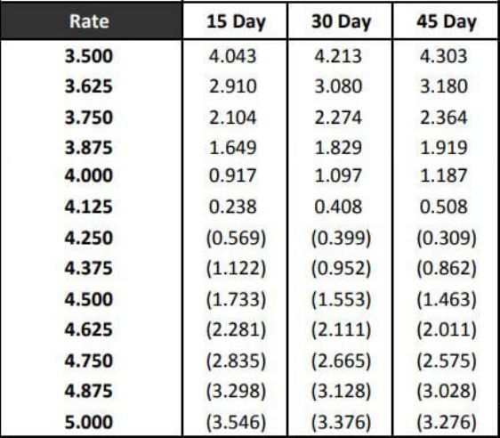
Figure 1: Rate and upfront closing costs options in an example lender rate sheet

Note: Figure 1 shows a set of rate and upfront closing costs options available to borrowers from an example wholesale lender

ratesheet. The ﬁrst column indicates the rate, while the next three columns shows the amount of upfront closing costs, in

the form of points/percentages of the loan amount, the borrower would have to pay to lock the rate for 15, 30, or 45 days,

respectively. Negative points are also possible in order to cover the other upfront closing costs the borrowers might have to pay.

Figure A.1 shows an example of how a price comparison website displayed the series of rate and upfront closing cost choices.

Figure 2: Kaplan-Meier survival hazards with months of interest rate incentive being greater

than 1.2%

Note: The data used in this ﬁgure is the Optimal Blue-HMDA-CRISM data from January 2013 to May 2022, for 30-year, ﬁxed-

rate, conforming, primary residence mortgages originated in 2013–2019. The green line Figure 2 presents the Kaplan-Meier

survival estimates of prepayment for mortgages with a reﬁnancing incentive, here deﬁned as a Freddie Mac survey rate decrease,

of greater than or equal to 1.2%. The red line in Figure 2 shows the result of the same analysis among borrowers with an

Equifax Risk Score that is above 700 and an estimated loan-to-value ratio of below 80% throught the sample, which is a group

of borrowers who are unlikely to face supply-side constraints in reﬁnancing. CRISM data is attributed to Equifax Credit Risks

Insight Servicing and Black Knight McDash Data.

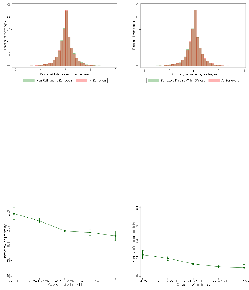
Figure 3: Points paid by borrower prepayment behavior

(a) Reﬁnancing behavior (b) Prepayment behavior

Note: The data used in this ﬁgure is the Optimal Blue-HMDA-CRISM data from January 2013 to May 2022, for 30-year, ﬁxed-

rate, conforming, primary residence mortgages originated in 2013–2019. Figure 3a presents a histogram of borrower choices of

points demeaned by lender by county by year groups, comparing between non-reﬁnancing borrowers (deﬁned as borrowers who

did not reﬁnance or otherwise prepay within ﬁve years despite facing a Freddie Mac Survey Rate decrease of at least 1.2%) and

all borrowers who faced a Freddie Mac Survey Rate decrease of at least 1.2%. Figure 3b conducts the same analysis comparing

borrowers who prepaid within ﬁve years versus all mortgages that have been originated for at least ﬁve years. CRISM data is

attributed to Equifax Credit Risks Insight Servicing and Black Knight McDash Data.

Figure 4: Moving/reﬁnancing probability by points paid

(a) Moving probability by points (b) Reﬁnancing probability by points

Note: The data used in this ﬁgure is the Optimal Blue-CRISM data from January 2013 to May 2022, for 30-year, ﬁxed-rate,

conforming, primary residence mortgages originated in 2013–2019. CRISM data is attributed to Equifax Credit Risks Insight

Servicing and Black Knight McDash Data. Figure 4a presents the predicted probabilities in regressions of moving on control

variables, while Figure 4b presents the predicted proabilities in regressions of reﬁnancing on control variables. The regression

estimates that these results were based on are presented in Table 2.

Figure 5: Market interest rate vs no cross-subsidization counterfactual interest rate for the

calibrated quick to reﬁnance borrower

Note: Figure 5 presents the equilibrium rate and upfront closing costs trade-oﬀ from the model and compares it to the empirical

rate and upfront closing costs trade-oﬀ that I estimate from the data. The “Market rate, model implied” solid line refers to the

equilibrium rate and closing cost trade-oﬀ given the logit prepayment hazard function and our estimated OAS. The “Market

rate, empirical” dotted line was estimated using a regression of rate on upfront closing costs with ratesheet ﬁxed eﬀects using the

LoanSifter data. Finally, the “No cross-subsidization counterfactual” dashed line refers to the model-implied equilibrium rate

and closing cost trade-oﬀ in a world where the lender is pricing their mortgages for the calibrated quick to reﬁnance borrower

with perfect information on their type. This counterfactual was computed by jointly iterating on the borrower and lender’s

value functions.

Figure 6: Welfare relative to no cross-subsidization counterfactual, calibrated quick to reﬁ-

nance borrower

Note: Figure 6 plots (i) the upfront cash the calibrated quick to reﬁnance borrower would have to receive to remain indiﬀerent

in the no cross-subsidization counterfactual, (ii) the upfront cash the lender’s diﬀerence in proﬁt from the quick to reﬁnance

borrower’s loan between the current world and the no cross-subsidization counterfactual, and (iii) the sum of (i) and (ii). The

results suggests that under the current system, the quick to reﬁnance borrower gains 2.4% of loan amount in dollar terms,

whereas lender loses 5.5% of the loan amount in proﬁt, with a total social loss of 3.0% of the loan amount.

Figure 7: Distribution of borrower reﬁnancing types

(a) Probability of being able to reﬁ (b) Hassle cost for reﬁnancing

Note: Figure 7a plots the estimated density for the probability of being able to reﬁnance coming from the marginal of the

multivariate Logit-Normal distribution of Equation (19). Figure 7b plots the estimated density for the hassle cost of reﬁnancing

from the Log-Normal distribution of Equation (21). The distribution of borrower types from all racial groups are included.

Figure 8: Discount factor and its correlation with reﬁnancing ability

(a) Discount factor

(b) Scatter plot of the probability of being able

to reﬁ and discount factor

Note: Figure 8a plots the estimated density for the discount factor coming from the marginal of the multivariate logit-Normal

distribution of Equation (19). Figure 8b plots a scatter plot with simulated draws of p

in the x-axis and β

in the y-axis from

the multivariate logit-Normal distribution of Equation (19) across all racial groups.

Figure 9: Moving probability

Note: Figure 9 plots the estimated density of moving probabilities across borrower types from the logit-Normal distribution of

Equation (20) across all racial groups.

Figure 10: Diﬀerences in utility in the actual world versus the perfect information benchmark

(a) Raw Density

(b) By borrower reﬁnancing ability

Note: Figure 10a plots the estimated density of the diﬀerence in utility, in terms of upfront dollar savings, that would make

borrowers indiﬀerent between the existing system and what they would otherwise obtain in the perfect information case.

Figure 11: Welfare eﬀects of cross-subsidization by racial group

Note: Figure 11 plots the average diﬀerence in utility due to the cross-subsidization by racial group. Utility is expressed in

terms of the upfront dollar savings that would make borrowers indiﬀerent between the existing system and what they would

otherwise obtain in the perfect information case.

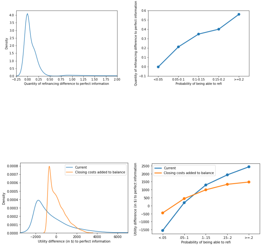
Figure 12: Diﬀerences in the expected number of reﬁnances in the actual world versus the

perfect information benchmark

(a) Raw Density (b) By borrower reﬁnancing ability

Note: Figure 12 plots the estimated density of the diﬀerence in the quantity of reﬁnancing per new origination between the

current system and the perfect information world where lenders price the rate and upfront closing cost trade-oﬀ with full

knowledge of borrower parameters and borrowers optimizing accordingly.

Figure 13: Counterfactual utility from adding cost to balance

(a) Distribution

(b) By borrower reﬁnancing ability

Note: Figure 13a plots the estimated density of the diﬀerence in utility, in terms of upfront dollar savings, that would make

borrowers indiﬀerent between the existing system and what they would otherwise obtain in the perfect information case.

Figure 14: Counterfactual utility from automatically reﬁnancing

(a) Distribution

(b) By borrower reﬁnancing ability

Note: Figure 14a plots the estimated density of the diﬀerence in utility, in terms of upfront dollar savings, that would make

borrowers indiﬀerent between the existing system and what they would otherwise obtain in the perfect information case, for the

automatically reﬁnancing counterfactual (in orange) as compared to the current system (in blue, reproduced from Figure 10).

Appendix

This appendix supplements the empirical analysis of Zhang (2023). Below is a list of the

sections contained in this appendix.

Table of Contents

A.1 Additional Background About Rate and Upfront Closing Costs 3

A.2 Data Construction and Summary Statistics 4

A.2.1 Optimal Blue-HMDA sample . . . . . . . . . . . . . . . . . . . . . . . 4

A.2.2 Optimal Blue-HMDA-CRISM sample . . . . . . . . . . . . . . . . . . . 6

A.2.3 The LoanSifter data . . . . . . . . . . . . . . . . . . . . . . . . . . . . 8

A.3 When are cl osing costs added to the rate? 9

A.4 Additional motivating facts 13

A.4.1 Regression of choices of points as predicted by ex-post prepayment be-

havior . . . . . . . . . . . . . . . . . . . . . . . . . . . . . . . . . . . . 14

A.4.2 Prevalence of mortgages with closing costs added to the rate . . . . . . 14

A.4.3 Cross-subsidization of closing costs added to the rate . . . . . . . . . . 21

A.4.4 The predictability of cross-subsidization by demographics . . . . . . . . 23

A.5 Robustness check on the proportion of closing costs paid upfront 26

A.6 Model details 26

A.6.1 Exogenous states . . . . . . . . . . . . . . . . . . . . . . . . . . . . . . 26

A.6.2 OAS . . . . . . . . . . . . . . . . . . . . . . . . . . . . . . . . . . . . . 28

A.6.3 Economic intuition on transfers and ineﬃciencies . . . . . . . . . . . . 31

A.7 Estimates by race 32

A.1 Additional Background About Rate and Upfront

Closing Costs

Figure A.1: Rate and upfront closing costs trade-oﬀs facing mortgage borrowers



®











 

    

@







 

    



    







2.740







$3750





$1563











Note: Figure A.1 shows a screenshot obtained by the author from Bankrate.com for a $250,000 reﬁnancing mortgage on

September 18, 2021. It shows how a borrower may choose to pay 0 points for a 2.740% interest rate mortgage, 0.626 points for

a 2.615% interest rate mortgage, or 1.5 points for a 2.490% interest rate mortgage.

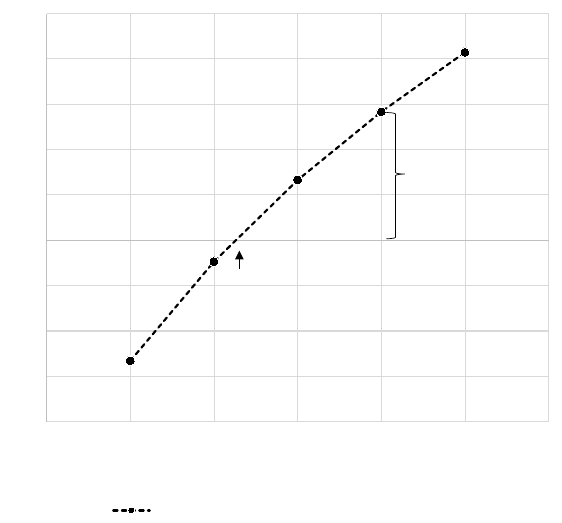
Figure A.2: Secondary marketing income as a function of interest rates

-8

-6

-4

-2

2.5 3 3.5 4 4.5 5 5.5

Price premium relative to par (percent of loan amount)

Interest rate

Secondary marketing income based on MBS TBA prices

secondary

marketing

income

MBS

yield

Note: Figure A.2 plots the FNMA MBS TBA prices on January 2, 2014 expressed as a percentage point premium/discount

over the loan amount on the y-axis for a variety of coupon rates on the x-axis. Secondary marketing income is the extent to

which the secondary market value of the mortgage is above its principal balance.

A.2 Data Construction and Summary Statistics

A.2.1 Optimal Blue-HMDA sample

I constructed the Optimal Blue-HMDA sample by merging the Optimal Blue rate locks from

2018–2019 with the public HMDA data. Because Optimal Blue contains a lender identiﬁer

number but no lender names, the merge proceeds in two steps: (1) an initial match based

on loan characteristics, and (2) a second ﬁltering based on a correspondence between the

lender identiﬁer in Optimal Blue and an anonymized version of HMDA lender IDs implied

by the ﬁrst step.

The initial match was made using loan amount, rate, year, loan type, loan purpose, loan

term, ZIP code (with all ZIP codes corresponding to an HMDA census tract included), and

up to a 5% diﬀerence in LTV with all matches kept in the data set. Then, for the second

step I impose the requirement that the lender identiﬁer in Optimal Blue is matched to an

anonymized version of HMDA lender ID at least 10% of the time.

Overall, this two-step

procedure uniquely matches 1,186,906 out of 2,318,940 locks for 30-year, conforming ﬁxed-

rate mortgages, implying a match rate of 51%. The match rate is comparable to a 66% “lock

pull-through rate,” which is the percent of rate locks that turn into originated loans, that I

understand to be reasonable based on industry sources.

In terms of variable deﬁnitions, I construct a Black dummy equal to one if the mortgage

has a HMDA-derived race variable of “Black or African American.” The Hispanic dummy is

equal to one if the mortgage has a HMDA derived ethnicity variable of “Hispanic or Latino.”

The Single Male and Single Female dummies are inferred from the HMDA-derived gender.

Summary statistics for these samples are shown in the table below.

The 10% requirement was set purposefully low to include cases where the Optimal Blue lender ID may

not correspond to a HMDA reporter for example in the case of correspondent lending. It is suﬃcient to

reduce the percent of matches that are non-unique from 49.6% to 3.9%.

Table A.1: Summary statistics for the 2018–2019 Optimal Blue-HMDA sample

All Black Hispanic

Mean Std. Dev. Mean Std. Dev. Mean Std. Dev.

Loan amount ($’000s) 256695.6 117785.7 242574.6 117351.2 243938.2 112333.0

Origination cost ($) 1516.0 1807.2 1657.6 2062.3 1849.0 1969.4

Total loan cost ($) 3902.6 2362.4 4222.6 2713.2 4487.1 2547.2

LTV (%) 747.9 44.5 728.7 47.3 732.7 45.5

DTI (%) 80.4 15.0 84.9 13.5 82.6 14.7

Interest rate 34.973 9.681 37.363 8.849 38.239 8.600

Points paid 4.544 0.579 4.692 0.612 4.674 0.603

First-time home buyer (d) 0.307 0.461 0.395 0.489 0.387 0.487

Single Female (d) 0.252 0.434 0.436 0.496 0.268 0.443

Single Male (d) 0.330 0.470 0.356 0.479 0.441 0.497

# Observations 1,041,807 42,793 92,598

Notes: This table reports summary statistics from the 2018–2019 Optimal Blue-HMDA merged

sample. Loan amount is expressed in thousands of dollars, origination costs are expressed in dollars,

credit score is the borrower’s Optimal Blue credit score at origination, and LTV, interest rate are

expressed in percentage points. The label (d) denotes dummy variables.

A.2.2 Optimal Blue-HMDA-CRISM sample

I also construct a merge between Optimal Blue, HMDA, and CRISM data sets for mortgages

originated between 2013–2019, with loan performance until May 2022. The CRISM data

set is an anonymous credit ﬁle match from Equifax consumer credit database to Black

Knight’s Mcdash loan-level Mortgage Data set. My Optimal Blue-HMDA-CRISM sample

was constructed by joining together three merges, (i) the 2018–2019 Optimal Blue and

HMDA merge described in Section A.2.1, (ii) a 2013–2017 Optimal Blue and HMDA merge,

and (iii) the 2013–2019 Optimal Blue and CRISM merge.

Similar to the 2018-2019 Optimal Blue and HMDA merge, the 2013–2017 Optimal Blue

and HMDA merge was also conducted in two steps, with an initial step based on loan

characteristics, and a second step based on a correspondence between the Optimal Blue

lender ID and an anonymized HMDA lender ID. A separate merge was conducted because the

data ﬁelds in 2013–2017 HMDA are diﬀerent than those in 2018–2019 HMDA: the interest

rate, loan term, and LTV ﬁelds were not available, while loan amount was given in ﬁner

detail.

The ﬁrst step for the 2013–2017 Optimal Blue to HMDA match was made using loan

amount, year, loan type, loan purpose, occupancy, ZIP code (with all ZIP codes correspond-

ing to an HMDA census tract included) with all matches kept in the data set. Then, for the

second step I impose the requirement that the lender identiﬁer in Optimal Blue is matched

to an HMDA respondent ID at least 10% of the time.

Overall, this two-step procedure

uniquely matches 1,382,057 out of 2,563,550 locks for 30-year, conforming ﬁxed-rate mort-

gages, implying a match rate between locks to originated mortgages of 54%. The match rate

is again comparable to a 66% “lock pull-through rate,” which I understand to be reasonable

based on industry sources.

The 2013–2019 Optimal Blue to CRISM match was made in one step. The variables

used for matching are the loan amount, ZIP code, month of origination (which I require

to lie within the date of the lock and the date of the lock plus the lock term), loan type,

loan term, loan purpose, Equifax Risk Score (within 20 points of the Optimal Blue credit

score), LTV (within 5%), and the rate. The more detailed loan-level information enabled the

match to proceed despite not having lender information. Overall, I uniquely matched 617,058

out of 5,269,107 locks for 30-year, conforming ﬁxed-rate mortgages, implying a match rate

between locks to originated mortgages in the CRISM data set of 12%. The lower match

rate is reasonable because neither the CRISM data nor the Optimal Blue data covers all

The 10% requirement was set purposefully low to include cases where the Optimal Blue lender ID may

not correspond to an HMDA reporter for example in the case of correspondent lending. It is suﬃcient to

reduce the percent of matches that are non-unique from 75.2% to 11.8%.

US mortgage originations, so the overlap between the two must be smaller than the overlap

between Optimal Blue and HMDA as the HMDA does provide essentially complete coverage

of all US mortgage originations.

Combining the three merges, I get an Optimal Blue-HMDA-CRISM sample with 360,291

loans. In terms of variable deﬁnitions, I construct a Black dummy equal to one if the

mortgage has a 2018–2019 HMDA derived race variable of “Black or African American.”

The Hispanic dummy is equal to one if the mortgage has a HMDA derived ethnicity variable

of “Hispanic or Latino.” In the case of 2013–2017 HMDA, these dummies are deﬁned using

the algorithm of Bhutta and Canner (2013). The Single Male and Single Female dummies

are inferred from the 2018–2019 HMDA derived gender or the applicant gender when no

co-applicant is present in the case of 2013–2017 HMDA. Finally, the Credit Card Revolver

dummy is set equal to 1 if the primary borrower on the mortgage has a credit card balance

of greater than or equal to $10,000 at the time of origination while also having a credit card

utilization of greater than 40%.

Summary statistics on this sample is shown in Table 1.

A.2.3 The LoanSifter data

The LoanSifter data contains information about rate and upfront closing cost (i.e., points)

trade-oﬀs in rate sheets, which are prices that loan originators and mortgage brokers can oﬀer

to clients in locking the loan. Because these are actual available prices within a lender, they

allow me to observe the rate and point menus that borrowers face. The sample period runs

from September 9, 2009 to December 31, 2014 and consists of rate sheets from a sample of

lenders from 50 metropolitan areas. Rate sheets observations are at the lender-day level, and

in rare cases where a lender issues more than one rate sheet on a given day the observations

with the best prices are kept. Linear interpolation was used to estimate the rate at various

levels of points, following Fuster, Lo, and Willen (2017). To compare the rate and points

menus in the lender rate sheets to the MBS TBA prices, I focus on rate sheets for conforming,

30-year, ﬁxed-rate mortgages with a loan-to-value ratio of 80% and a loan amount of greater

than or equal to $300k.

Summary statistics for this data are shown in Table A.2.

Table A.2: Summary statistics for the LoanSifter data

Year No. of Lenders Rate at -2 points Rate at 0 points Rate at 2 points N lender-days obs

2009 93 5.42 5.01 4.65 3923

2010 93 5.10 4.70 4.44 16025

2011 83 4.82 4.46 4.25 16589

2012 86 4.07 3.67 3.41 18105

2013 126 4.42 4.07 3.80 19993

2014 103 4.52 4.21 3.97 19446

Note: This table contains information on the number of distinct lenders, mean rate at 0 points, mean

rate at 2 points, and number of distinct lender-day observations by year. The data set comes from

LoanSifter. The interest rates at 0 points and at 2 points are estimated through linear interpolation

for lenders that do not oﬀer mortgages at exactly those points.

A.3 When are closing costs added to the rate?

This paper focuses on the cross-subsidization of mortgage closing costs to the extent that they

are added to the rate of the mortgage. I refer to mortgages with closing costs “added to the

rate” as mortgages with a high enough interest rate c such that secondary marketing income(c)

in Equation (1) is positive.

While intuitive, this deﬁnition is most sensible in a world in

which lenders pass through their secondary marketing income as lower upfront closing costs

to borrowers, for example in a model with a perfectly competitive supply side. Otherwise,

the positive secondary marketing income may reﬂect not only closing costs added to the rate

but also an additional cost that only some borrowers pay. Empirically, my analysis of US

This turns out to be true for most mortgages, as I show in Section A.4.2.

mortgage pricing ﬁnds this pass-through to be nearly complete which makes my deﬁnition

sensible.

To assess this pass-through, I examine how the secondary marketing income-interest rate

trade-oﬀ matches the retail interest rate and upfront closing costs trade-oﬀ in the cross-

section, with results in Figure A.3. I use data LoanSifter matched with MBS TBA pricing

data from 2009Q3 to 2014. Following the methodology of Fuster, Lo, and Willen (2017),

which estimates the price of intermediation as the premium of the mortgage over par on

the secondary market, I estimate (i) the secondary marketing revenue generated by lenders

in the secondary market as implied by MBS TBA prices, and (ii) the sum of the revenue

generated by lenders in the secondary market and the upfront closing costs they charge in

the form of points, for borrowers with a $300k conforming mortgage, 700 LoanSifter credit

score, 80% LTV, and 30% DTI.

Then, with the interest rate spread to the Freddie Mac Primary Mortgage Market Survey

(PMMS) rate

rounded to the nearest 1/8th ˜c, I run a linear regressions of the form:

ijt

l=1

(c = c

) + ξ

+ 

ijt

, (27)

where c

are the categorical variables of interest rate spread rounded to the nearest 1/8th, ξ

are lender-day ﬁxed eﬀects, and 

ijt

is the error term. φ

ijt

is either the secondary marketing

revenue generated the lender or sum of the revenue generated by lenders in the secondary

market and the upfront closing costs, both expressed as a percentage of the loan amount.

Results are presented in Figure A.3, which shows that mortgages that are originated at

a higher spread to the Freddie Mac Survey rate tend to command higher valuations in the

secondary market but generate almost exactly the same lender total income. This suggests

that higher secondary marketing income is almost entirely passed through to consumers

in the form of lower upfront lender fees/points.

Given the near complete pass-through

The Freddie Mac Primary Mortgage Market Survey rate is obtained from

https://fred.stlouisfed.org/series/MORTGAGE30US.

The same patterns also exist in the time series, as I illustrate in Appendix Figure A.4. In Figure A.4,

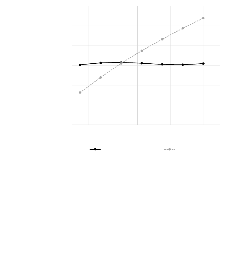
of secondary marketing income to primary market upfront closing costs on average, it is

economically meaningful to say that mortgages with positive secondary marketing income

have a part of their upfront closing costs “added to the rate” which is then subject to

cross-subsidization.

Figure A.3: Secondary marketing income and total lender revenues

-0.3 -0.2 -0.1 0 0.1 0.2 0.3 0.4 0.5 0.6

Percent of Loan Amount

Interest rate spread to Freddie Mac Survey Rate

MBS TBA Value + Points MBS TBA value

Note: Figure A.3 presents estimates from a linear regression of (i) the estimated secondary marketing revenue as implied by

MBS TBA prices and (ii) the sum of estimated secondary marketing revenue as implied by MBS TBA prices and upfront

closing costs in the form of points on categorical variables of eighths of rate spreads with lender-day ﬁxed-eﬀects based on

Equation (27). The grey dotted line plots the predicted values from the regression with estimated secondary marketing revenue

as the regressor. The black solid line plots the predicted values from the same regression on the sum of estimated secondary

marketing revenue and upfront closing costs in the form of points.

In addition to cross-section, I also examine the relationship between the rate and upfront

closing cost trade-oﬀ in the time series in Figure A.4. Using the LoanSifter data, I estimate

the rate increase from paying 1 less point (i.e., 1% of the loan amount less) in upfront closing

there is some evidence that in more recent years the interest rate is slightly lower on low upfront closing

cost mortgages than what would be implied by secondary marketing income, perhaps suggesting a role

for markups. I abstract from markups that vary by points in this paper as the magnitude of the cross-

subsidization I study is signiﬁcantly larger than the diﬀerences shown in Figure A.4.

costs as the interest rate increase from going from a mortgage with 1 point in upfront closing

costs to a mortgage with 0 points within each lender rate sheet. To get the corresponding

exchange rate in the MBS TBA data, I take the mortgage rate at 0 points (net of the g-fees

or the price of GSE guarantee) and compute the increase in rate that would imply a 1%

increase in the MBS TBA value of the mortgage, with interpolated values for coupon rates

in between eighths. I then take the mean of the exchange rate implied by the LoanSifter

data and the MBS TBA data by month, with results plotted in Figure A.4.

Figure A.4: The interest rate increase from paying 1 less point in upfront closing cost over

time, lender ratesheets (green) versus MBS TBA implied (red)

.1 .15 .2 .25 .3

Rate increase from paying 1 fewer point

2009m7 2010m7 2011m7 2012m7 2013m7 2014m7

month

MBS TBA implied Lender Ratesheets

Note: Figure A.4 presents estimates from taking monthly means of (i) the required increase in rate to make the mortgage value

increase by 1% of the loan amount in the MBS TBA data (ii) the increase in rate going from 0 points in lender rate sheet to 1

point in lender rate sheet in terms of upfront closing costs paid. The data used is Morgan Markets for MBS TBA prices and

LoanSifter for rate sheets. MBS TBA values are linearly interpolated in between eighths of interest rates and LoanSifter rates

are linearly interpolated to arrive at the rate at 0 and 1 point in upfront closing costs.

Figure A.4 shows that the exchange rate implied by the the LoanSifter data and the

MBS TBA data are fairly close to each other, with the MBS TBA implied exchange rate

being slightly larger near the end of the sample. This is consistent with near complete pass-

through of secondary marketing revenue to upfront closing costs, with a small discount to

lower closing cost mortgages in the retail market as compared to the secondary market near

the end of the sample.

A.4 Additional motivating facts

In this section, I present some additional stylized facts that illustrate the existence of cross-

subsidization of mortgage closing costs and its sizable distributional implications. First,

I show in Section A.4.2 that almost all borrowers pay for most of their mortgage closing

costs through a higher interest rate on their mortgage relative to mortgage-backed securi-

ties yields, rather than upfront. Second, I show that heterogenous borrower prepayment

tendencies implies diﬀerent borrowers with the same closing costs added to the rate end

up with very diﬀerent net present values (NPVs) of their extra interest rate payments, ex

post, in Section A.4.3. Third, I assess magnitude of this diﬀerence by demographic groups

in Section A.4.4.

A.4.1 Regression of choices of points as predicted by ex-post pre-

payment behavior

Table A.3: Choices of points as it relates to reﬁnancing/prepayment behavior

(1) (2)

Points Points

Non-reﬁ borrower 0.0659

∗∗∗

(5.32)

5-year prepayment -0.0841

∗∗∗

(-6.30)

Log(loan amount) 0.0511

∗∗∗

(2.71) 0.0497

∗∗∗

(2.73)

Credit score controls Yes Yes

LTV controls Yes Yes

DTI control Yes Yes

Constant -0.600

∗∗∗

(-2.83) -0.519

∗∗

(-2.59)

Observations 25245 25245

LenderXCountyXYear FEs Yes Yes

Robust t statistics clustered by lender and county in parentheses.

* p<0.1, ** p<0.05, *** p<0.01

Note: The data used in this ﬁgure is the Optimal Blue-HMDA-CRISM data from January 2013 to May 2022, for 30-year,

ﬁxed-rate, conforming, primary residence mortgages originated in 2013–2019. The sample for (1) and (2) is further restricted

to the set of borrowers whose mortgages originated before April 2016 and where the Freddie Mac Survey Rate decreased at

least 1.2% since origination. Table A.3 presents OLS estimates of borrower choices of points on (1) an indicator variable for

non-reﬁnancing borrowers, deﬁned as borrowers who did not reﬁnance or otherwise prepay within ﬁve years despite facing a

Freddie Mac Survey Rate decrease of at least 1.2%, and (2) borrowers who prepaid within ﬁve years.

A.4.2 Prevalence of mortgages with closing costs added to the

rate

When borrowers take out a mortgage, they have a choice between adding closing costs to

the rate of the mortgage or paying them upfront. In this section I assess the extent to which

mortgage closing costs are added to the rate using the 2018–2019 Optimal Blue-HMDA data.

The 2018–2019 HMDA data contains information about the upfront closing costs paid by the

borrower in the form of loan origination costs, and the match to Optimal Blue data enables

me to obtain information on when the rate was locked which then allows me to estimate the

revenue that lenders generate from the secondary market.

I estimate the extent to which mortgage closing costs are added to the rate based on

Equation (1), which breaks down lenders’ total revenue from origination as the sum of

upfront closing costs and secondary marketing income. The secondary marketing component

of lender revenues is estimated following the procedure of Fuster, Lo, and Willen (2017),

where the revenue that lenders generate from the secondary market y as a fraction of the

mortgage balance M

is given as:

T BA+payup

− gfees

) − M

(28)

where p

T BA+payup

is the estimated value of the mortgage on the secondary market based on

TBA prices plus “payups,” for a coupon rate c

− gfees

where c

is the interest rate on

the mortgage and gfees

is the price of the government guarantee. Payups are additional

amounts that investors pay for an MBS relative to the TBA price for mortgages that have

particularly favorable prepayment risk. Low-balance mortgages, for example, are less likely

to be prepaid and hence tend to be more valuable in the secondary market. As a result, I

add the payups based on mortgage size to the MBS TBA price.

The methodology of Fuster, Lo, and Willen (2017) for estimating secondary marketing income involves

estimating the premium of an originated mortgage relative to par from MBS TBA prices by subtracting g-

fees (the cost of GSE guarantee) from the mortgage interest rate and then using that as the coupon rate, the

value of which is then derived using linear interpolation on reported MBS TBA prices between (i) coupons

and (ii) trading days.

A drawback of this approach of estimating secondary marketing income is that it excludes both the

impact of the revenue generated from the sale of mortgage servicing rights and the fees paid to servicers

from coupon payments. Fuster, Lo, and Willen (2017) argue that the two eﬀects may approximately cancel

each other out. Without explicit data on the value of mortgage servicing rights, I also compute a lower bound

on the estimated lender revenues by looking at the MBS value of the net interest rate paid to investors by

assuming counterfactually that mortgage servicing rights are worth zero. This lower bound is presented in

Appendix Figure A.13, which still shows that the vast majority of mortgages have their closing costs paid

for through the rate.

The results of my analysis are shown in Figure A.5. The left panel in Figure A.6a shows

that lenders make on average 4.6% of the mortgage balance as revenue for each mortgage they

originate. This revenue compensates the lender for their costs. First, lenders need to pay for

the upfront costs of mortgage insurance, also called loan-level price adjustments (LLPAs) by

Fannie Mae and Freddie Mac. Second, lenders pay for loan originator compensation, which

can be 1–2% of the loan amount. Third, lenders pay for the underwriting and processing costs

associated with the origination. Relative to these expenses, the portion that is attributable

to accounting proﬁts are low: the Mortgage Bankers’ Association (MBA) reports an average

production proﬁt of 0.14% of the loan amount in 2018 and 0.31% of the loan amount in

2017.

The right panel of Figure A.5b shows that only a small fraction of lender revenue is paid

as upfront closing costs, with an average of 17.4%. That is, even though most of the lender

costs of origination are incurred upfront, 82.6% of the price of origination is added to the

rate of the mortgage and paid over time primarily by immobile and inactively reﬁnancing

borrowers. Hence, almost all mortgages being originated in the US can be considered “low

upfront closing cost” mortgages whose price of mortgage origination are prone to cross-

subsidization between borrowers with diﬀerent reﬁnancing speeds.

https://www.mba.org/2019-press-releases/april/independent-mortgage-bankers-production-volume-

and-proﬁts-down-in-2018. MBA also reports that average net production revenues in 2018 (excluding

LLPAs) are 3.47% of the loan amount, which is consistent with my estimate of 4.6% with LLPAs.

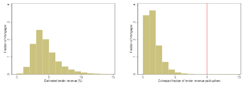
Figure A.5: Lender revenue and percentage paid as upfront closing costs

(a) Estimated lender revenue (b) Fraction of lender revenue paid upfront

Note: The data used in this ﬁgure is the 2018–2019 Optimal Blue-HMDA data for 30-year, ﬁxed-rate, conforming, primary

residence mortgages originated. The data contains information on rates and upfront closing costs paid and was linked to MBS

TBA data following Fuster, Lo, and Willen (2017) to estimated secondary marketing revenue. Figure A.6a plots histograms

of estimated lender revenue which consists of the sum of upfront closing costs plus secondary marketing revenue. Figure A.5b

then plots histograms of the fraction of lender revenue that is paid upfront.

Conceptually, the empirical observation that lenders make most of their income from

secondary marketing revenue is best characterized as closing costs being added to the rate if

higher secondary marketing revenue is passed through to consumers as lower upfront closing

costs. I present evidence that this is true in Section A.3.

Table A.4: Total loan costs and loan balance

(1) (2) (3)

All Purchase Reﬁ

Loan amount in dollars 0.00504

∗∗∗

0.00640

∗∗∗

0.00132

∗∗∗

(14.38) (18.61) (3.05)

Constant 2595.5

∗∗∗

2378.4

∗∗∗

3172.8

∗∗∗

(28.24) (23.93) (30.40)

Observations 1154560 899391 255169

Robust t statistics clustered by lender and county in parentheses.

* p<0.1, ** p<0.05, *** p<0.01

Note: The data used in this ﬁgure is the 2018-2019 Optimal Blue-HMDA data, for 30-year, ﬁxed-rate, conforming, primary

residence mortgages.

Table A.5: Upfront origination costs and loan balance

(1) (2) (3)

All Purchase Reﬁ

Loan amount in dollars 0.00146

∗∗∗

0.00191

∗∗∗

-0.000156

(6.01) (8.31) (-0.42)

Constant 1132.4

∗∗∗

984.6

∗∗∗

1702.0

∗∗∗

(19.32) (18.02) (17.88)

Observations 1154695 899504 255191

Robust t statistics clustered by lender and county in parentheses.

* p<0.1, ** p<0.05, *** p<0.01

Note: The data used in this ﬁgure is the 2018-2019 Optimal Blue-HMDA data, for 30-year, ﬁxed-rate, conforming, primary

residence mortgages.

Figure A.6: Lender revenue and percentage paid as upfront closing costs

(a) Estimated lender revenue (b) Fraction of lender revenue paid upfront

Note: The data used in this ﬁgure is the 2018–2019 Optimal Blue-HMDA data for 30-year, ﬁxed-rate, conforming, primary

residence mortgages originated. The data contains information on rates and upfront closing costs paid and was linked to MBS

TBA data following Fuster, Lo, and Willen (2017) to estimated secondary marketing revenue. Figure A.6a plots histograms

of estimated lender revenue which consists of the sum of upfront closing costs plus secondary marketing revenue. Figure A.5b

then plots histograms of the fraction of lender revenue that is paid upfront.

Figure A.7: Lender revenue and percentage paid as upfront closing costs

(a) Estimated lender revenue (b) Fraction of lender revenue paid upfront

Figure A.8: Total revenue and percentage paid as upfront closing costs, purchase

(a) Estimated lender revenue (b) Fraction of lender revenue paid upfront

Figure A.9: Lender revenue and percentage paid as upfront closing costs

(a) Estimated lender revenue (b) Fraction of lender revenue paid upfront

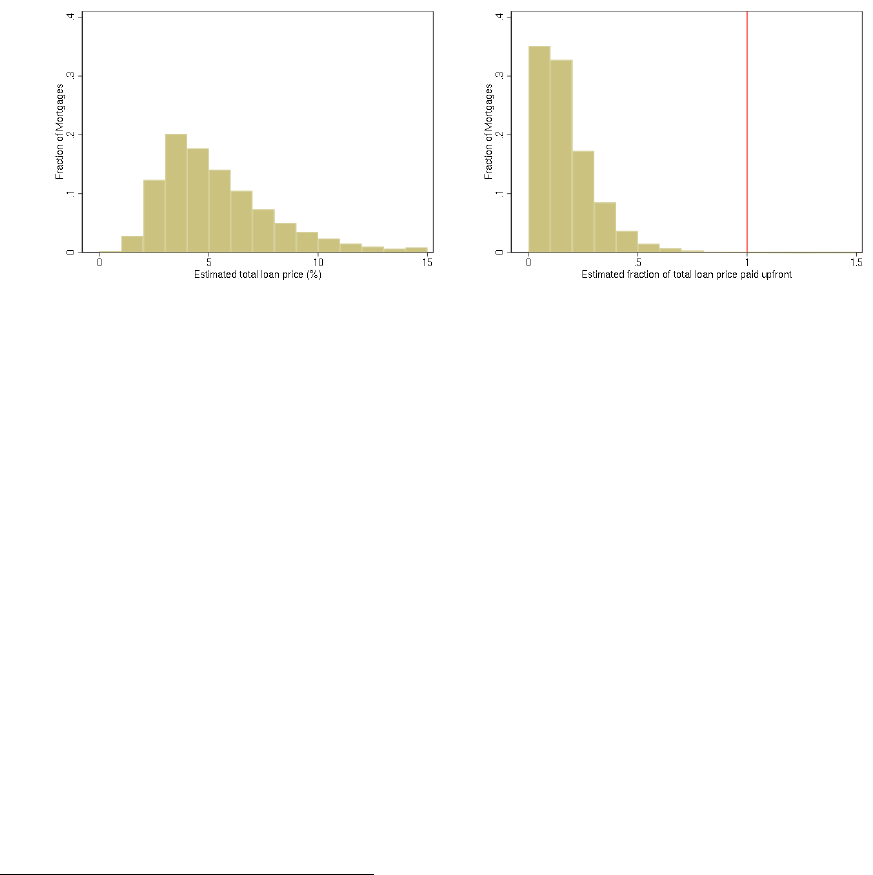
Figure A.10: Total revenue and percentage paid as upfront closing costs, reﬁ

(a) Estimated lender revenue (b) Fraction of lender revenue paid upfront

A.4.3 Cross-subsidization of closing costs added to the rate

The interaction of heterogeneity in reﬁnancing tendencies and closing costs added to the

rate implies a cross-subsidization of mortgage closing costs. To illustrate this in my data,

Figure A.11 looks at borrowers with similar amounts of closing costs added to the rate

(between 4.75-5.25%) in 2013 in my Optimal Blue-HMDA-CRISM sample and compares the

NPV of the extra interest rate they paid as a percentage of their loan amount.

Due to

diﬀerences in prepayment behavior, I ﬁnd large diﬀerences in how much borrowers end up

paying for the 4.75-5.25% in closing costs they added to the rate, ranging from close to 0%

to more than 6%.

The year 2013 was chosen because it is the earliest year in my sample.

Figure A.11: NPV of extra interest paid, 2013 mortgages with 4.75–5.25% of the loan amount

in closing costs added to the rate

Note: The data used in this ﬁgure is the Optimal Blue-HMDA-CRISM data from January 2013 to May 2022, for 30-year,

ﬁxed-rate, conforming, primary residence mortgages originated in 2013. The sample was further limited to mortgages with a

secondary marketing revenue of 4.75–5.25% of the loan amount, as estimated based on MBS TBA prices following Fuster, Lo,

and Willen (2017). The rate increase relative to a mortgage with 0% secondary marketing revenue (i.e., at par) is estimated as

the diﬀerence between the mortgage interest rate net of the fee for government guarantee (gfees) minus MBS yields. The NPV

of the extra monthly payment resulting from this diﬀerence, assuming a discount rate equal to the 10-year Treasury rate at the

time of the rate lock, is then plotted in the histogram for loans that have prepaid (in green) and for loans that are still active

(in red). CRISM data is attributed to Equifax Credit Risks Insight Servicing and Black Knight McDash Data.

The reason for the variance in outcomes in Figure A.11 is that, when the closing costs

are added to the rate of the mortgage, lenders can only recover their closing costs over time

through a higher interest rate payment. The principal balance of the mortgage remains

unchanged. Therefore, borrowers who prepay earlier end up paying less, while borrowers

who prepay later end up paying more. The transfers and deadweight losses studied in this

paper come from the extent to which that borrowers who actively reﬁnance pay less for their

closing costs in expectation and receive cross-subsidization from other borrowers.

A.4.4 The predictability of cross-subsidization by demographics

Next, I examine the extent of this ex-post cross-subsidization by demographics. To do so, I

run the regression on loan level data in my Optimal Blue-HMDA-CRISM sample:

NP V

i,t

= βX

+ γZ

+ ξ

i,t

×t

+ 

i,t

(29)

where NP V

i,t

is the NPV of extra interest paid for their closing costs that are added to the

rate over the observed life of the mortgage; X

is a set of demographic and credit utilization

variables including race (Black, Hispanic), gender (male and female), credit card revolver

status, and quartiles of education; Z

is a set of control variables including categories of

credit scores at origination, LTV, DTI, and log loan amount; ξ

i,t

×t

is the amount of closing

costs added to the rate by time ﬁxed eﬀects.

The results of this analysis are shown in Figure A.12 and Table A.6. I ﬁnd that Black

and Hispanic borrowers paid an extra 0.5% of the loan amount for their closing costs added

to the rate relative to other borrowers. For a $300,000 loan, the magnitude of this cross-

subsidization is about $1500 per loan. Furthermore, single-applicant female borrowers paid

an extra 0.24% of the loan amount for their closing costs added to the rate. A limitation of

this analysis is that does not take into account the potentially unexpected decline in interest

rate during this period, so a model is needed to get at the welfare eﬀects ex ante.

Figure A.12: NPV of extra interest paid by demographic and borrower characteristics

Note: The data used in this ﬁgure is the Optimal Blue-HMDA-CRISM data from January 2013 to December 2013, for 30-year,

ﬁxed-rate, conforming, primary-residence mortgages originated in 2013. The graph plots regression coeﬃcients from Column (2)

of Table A.6. In particular, it shows that Black, Hispanic and single-applicant female borrowers pay more for their closing costs

added to the rate than other borrowers. Other characteristics, such as single-applicant male borrowers, ﬁrst-time home buyers,

credit card revolvers (deﬁned as someone with a more than 60% credit utilization and $10,000 in debt at the time of getting

a mortgage), and quartiles by education are not statistically diﬀerent from zero at the 5% level. CRISM data is attributed to

Equifax Credit Risks Insight Servicing and Black Knight McDash Data.

Table A.6: Regression on NPV of extra interest paid by demographic and borrower charac-

teristics

(1)

NPV of Extra Interest Paid

Black 0.434

∗∗∗

(2.17)

Hispanic 0.480

∗∗∗

(3.38)

Single male -0.042 (-0.40)

Single female 0.223

∗∗

(1.89)

First-time home buyer 0.078 (0.64)

Credit card revolver 0.091 (0.56)

1st quartile of education 0.101 (0.72)

2nd quartile of education 0.124 (0.85)

3rd quartile of education 0.098 (0.70)

Log(loan amount) -0.363

∗∗∗

(-2.92)

Credit Score controls Yes

LTV controls Yes

DTI control Yes

Constant 7.918

∗∗∗

(4.85)

Observations 1275

φ by month FEs Yes

robust t statistics in parentheses

* p<0.1, ** p<0.05, *** p<0.01

Note: The data used in this table is the Optimal Blue-HMDA-CRISM data from January 2013 to December 2013, for 30-year,

ﬁxed-rate, conforming, primary residence mortgages originated in 2013. This table contains regression results from estimating

Equation (28). The dependent variable is the NPV of extra interest paid from the closing costs that are added to the rate. I

include φ by month ﬁxed eﬀects, where φ refers to the amount of closing costs added to the rate rounded to the nearest percent

of the loan amount. CRISM data is attributed to Equifax Credit Risks Insight Servicing and Black Knight McDash Data.

A.5 Robustness check on the proportion of closing costs

paid upfront

Figure A.13: Lender revenue and percent paid as upfront closing costs, net of mortgage

servicing revenue

(a) Estimated lender revenue (b) Fraction of lender revenue paid upfront

Note: The data used in this ﬁgure is the Optimal Blue data for 30-year, ﬁxed-rate, conforming, primary residence mortgages

originated in 2018-2019 matched to the 2018–2019 HMDA data. This data contains information on rates and upfront closing

costs paid, and was linked to MBS TBA data to estimate secondary marketing revenue. A further 25 basis points was subtracted

from the coupon rate for mortgage servicing. Figure A.6a plots histograms of estimated lender revenue which consists of the

sum of upfront closing costs plus secondary marketing revenue. Figure A.13b then plots histograms of the fraction of lender

revenue that is paid upfront.

A.6 Model details

A.6.1 Exogenous states

The risk-free rate follows the Cox, Ingersoll, and Ross (1985) model which has a natural zero

lower bound:

= a(b − r

)dt + σ

√

. (30)

I estimate the evolution of exogenous states in the model via maximum likelihood

using

The program was based on Kladivko (2021), with some modiﬁcations to obtain standard errors.

the three-month Treasury bill data from January 1987 to January 2021.

The results for

the risk-free rate are as follows:

Table A.7: Estimation of the CIR model of interest rates

Parameter Estimate Standard Error

a 0.0910 0.0506

b 1.2649 0.7209

σ 0.4930 0.0175

Note: This table contains estimates from ﬁtting the Cox, Ingersoll, and Ross (1985) model on the three-month Treasury bill

data from January 1987 to January 2021. Estimation proceeds via the maximum likelihood, and standard errors are obtained

from the inverse Hessian.

I model the average mortgage rate ¯c

, changes in log real house prices ∆H

, and changes in

log real personal income ∆L

and as a vector autoregression (VAR) with r

as an exogenous

dependent variable. I use two lags in the VAR, with the constraint that the matrix of

coeﬃcients on ﬁrst lag is identity and on the second lag is positive only for the house price

coeﬃcient to reduce dimensionality.

More speciﬁcally, with s







¯c

100 ∗ ∆H

100 ∗ ∆L







, the VAR

equation is as follows:

= µ + r

+ Φ

t−1

+ Φ

∆H

t−1

+ e

, (31)

where e

∼ N(0,

) and µ, β

, Φ

are the coeﬃcients to be estimated. In terms of the state

variables, data on ¯c

is obtained as the Primary Mortgage Market Survey (PMMS) rate,

Board of Governors of the Federal Reserve System (US), 3-Month Treasury Bill Sec-

ondary Market Rate [TB3MS], retrieved from FRED, Federal Reserve Bank of St. Louis,

https://fred.stlouisfed.org/series/TB3MS.

The second lag on the house price variable is added to capture momentum and mean reversion as in

Glaeser and Nathanson (2017).

Freddie Mac, 30-Year Fixed Rate Mortgage Average in the United States [MORTGAGE30US], retrieved

from FRED, Federal Reserve Bank of St. Louis, https://fred.stlouisfed.org/series/MORTGAGE30US.

is obtained from the Case-Shiller National House Price Index,

and L

is obtained from

the US Personal Income

divided by the US population.

Furthermore, H

and L

are

converted to real terms using the Consumer Price Index for All Urban Consumers.

The

results of the VAR estimation are as follows:

Table A.8: VAR estimates of state transitions

Parameter µ β

¯c

.093 (.051) .024 (.010) .972 (.012) 0 0 0 .050

100 ∗ ∆H

.051 (.028) -.008 (.007) 0 1.060 (.047) 0 -.286 (.047) .009 .126

100 ∗ ∆L

.182 (.079) -.007 (.021) 0 0 -.232 (.053) 0 -.006 .041 1.030

Note: This table contains estimates from ﬁtting a constrained VAR described in Equation (31). Data on mean mortgage rates

¯c

is obtained from the Primary Mortgage Market Survey (PMMS), data on house prices H

are taken from the Case-Shiller

index, and data on personal income Y

are taken as the ratio of US aggregate personal income divided by the US population.

House prices and income are divided by the CPI for urban consumers and then transformed into log diﬀerences.

The estimates from Tables A.7 and A.8 are then used to simulate the transitions of the

exogenous states in my model in Section 5.

A.6.2 OAS

An empirical model of prepayment behavior combined with my model of interest rates is

needed to estimate the OAS in Section 5.1.2. For my empirical model of prepayment, I use

my panel data to estimate a logit regression of an indicator variable for borrower prepayment

on the spread of the mortgage interest rate to the Freddit Mac survey rate at origination

(SATO) as well as categories of the interest rate incentive deﬁned as the current mortgage

S&P Dow Jones Indices LLC, S&P/Case-Shiller U.S. National Home Price Index [CSUSHPINSA], re-

trieved from FRED, Federal Reserve Bank of St. Louis;,https://fred.stlouisfed.org/series/CSUSHPINSA.

U.S. Bureau of Economic Analysis, Personal Income [PI], retrieved from FRED, Federal Reserve Bank

of St. Louis, https://fred.stlouisfed.org/series/PI

U.S. Bureau of Economic Analysis, Population [POPTHM], retrieved from FRED, Federal Reserve Bank

of St. Louis, https://fred.stlouisfed.org/series/POPTHM.

U.S. Bureau of Labor Statistics, Consumer Price Index for All Urban Consumers: All Items

in U.S. City Average [CPIAUCSL], retrieved from FRED, Federal Reserve Bank of St. Louis,

https://fred.stlouisfed.org/series/CPIAUCSL.

interest rate minus the Freddit Mac survey rate. To maintain comparability to the TBA

market from which I derive the market exchange rate between the interest rate and upfront

closing costs, I further restrict my analysis to 30 year purchase mortgages with a balance

above $150k, FICO above 680, and LTV below 85% following Fusari et al. (2020). Results of

this regression are shown in Table A.9, which is used for my model of ˆp

as in Equation (17).

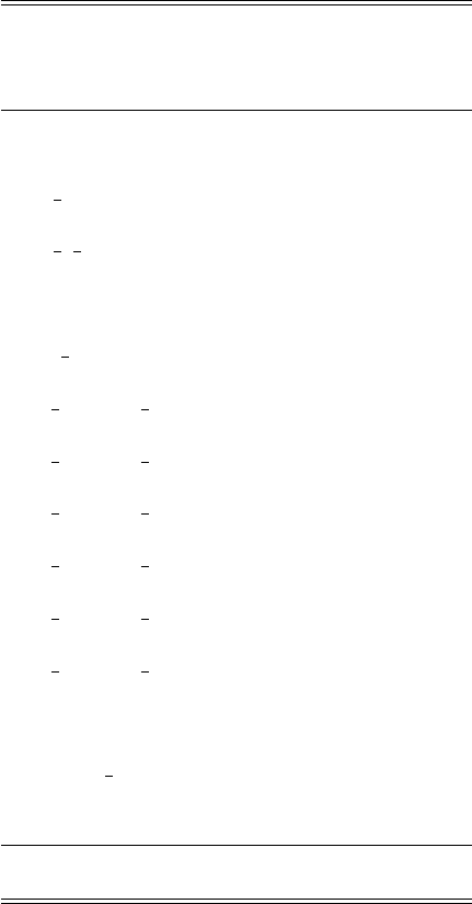
Table A.9: Logit model of prepayment

(1)

Logit

prepaid

init t 7.446

∗∗∗

(16.59)

init t sq -4.169

∗∗∗

(-12.32)

sato 0.121 (0.62)

sato sq -0.765

∗∗∗

(-2.88)

reﬁ ratediﬀ gt0 0.348

∗∗∗

(4.55)

reﬁ ratediﬀ gtp25 0.345

∗∗∗

(4.08)

reﬁ ratediﬀ gtp5 0.599

∗∗∗

(8.31)

reﬁ ratediﬀ gtp75 0.322

∗∗∗

(4.69)

reﬁ ratediﬀ gt1 0.538

∗∗∗

(5.63)

reﬁ ratediﬀ gt1p25 0.144 (1.09)

burnout -0.0549

∗

(-1.94)

burnout sq 0.00182 (1.45)

Constant -8.264

∗∗∗

(-54.48)

Observations 267603

t statistics in parentheses

∗

p < 0.1,

∗∗

p < 0.05,

∗∗∗

p < 0.01

Note: The data used in this regression is the Optimal Blue-HMDA-CRISM data from January 2013 to May 2022, for 30-year,

ﬁxed-rate, conforming, primary residence mortgages originated in 2013–2019. The sample is further restricted to “TBA likely”

mortgages deﬁned as mortgages with a loan amount of at least $150k, loan-to-value ratio less than or equal to 85%, and FICO

at origination greater than or equal to 680. The independent variable is an indicator variable for whether the borrower prepaid

their mortgage in a given month. The dependent variables include the spread of the mortgage interest rate to the Freddie Mac

survey rate at origination (SATO) and its square, as well as categories of rate incentive (the current spread of the mortgage

interest rate to the Freddie Mac survey rate). CRISM data is attributed to Equifax Credit Risks Insight Servicing and Black

Knight McDash Data.

Using the prepayment model from Table A.9 and the interest rate model of Section A.6.1,

with the risk-free rate r

being given as the implied 10 year rate under the Cox, Ingersoll,

and Ross (1985) model, I estimate a

OAS = 0.22% by minimizing the equally-weighted

diﬀerence between the observed MBS TBA price for the nearest two coupons above and

below the Freddie Mac survey rate - gfees - servicing fees with the implied NPV given by

Equation (17). The MBS TBA price is inclusive of the new production pay-up for a coupon

(with data from Morgan Markets). The gfee is assumed to be 0.42% and servicing fee 0.25%

following Fuster, Lo, and Willen (2017).

A.6.3 Economic intuition on transfers and ineﬃciencies

I showcase the economic intuition behind these results in Figure A.14, where I plot illustra-

tive demand curves for mortgage originations for a non-reﬁnancing borrower and an actively

reﬁnancing borrower. The demand curve for a non-reﬁnancing borrower is vertical, repre-

senting that their quantity of upfront closing is ﬁxed and due to exogenous factors (e.g.,

moving). The demand curve for an actively reﬁnancing borrower is downward sloping in the

price, representing the fact that an actively reﬁnancing borrower would reﬁnance more if

the price of originations is lower, as the interest rate savings from reﬁnancing become higher

than the price of a new origination.

The social marginal cost of mortgage origination is represented as a solid horizontal line.

For non-reﬁnancing borrowers, the price they face is this cost shifted upwards as the cost of

origination gets added to the rate and they end up paying more for each origination, which

is illustrated in Figure A.14a. For actively reﬁnancing borrowers, their eﬀective price of

mortgage origination is shifted downwards from the social cost, as illustrated in Figure A.14b.

An important distinction between the two panels is in the change of borrower behavior. To

the extent that actively reﬁnancing borrowers originate more mortgages than they otherwise

would due to this cross-subsidization, they introduce a social deadweight loss represented by

the triangle indicated by the arrow in Figure A.14b.

Figure A.14 may also be interpreted in terms of price elasticities. To the extent that

non-reﬁnancing borrowers’ quantity of mortgage origination are less price elastic, the eﬀect

of their cross-subsidization involves less of a change in behavior. Therefore, the economic

distortions in the model mostly attributed to the changes in the incentives faced by the

actively reﬁnancing borrowers who reﬁnance excessively.

Figure A.14: Deadweight loss from cross-subsidization of the price of mortgage reﬁnancing

(a) Non-reﬁnancing borrower

Price

Quantity of originations

Demand

Cost

(b) Actively reﬁnancing borrower

Price

Quantity of originations

deadweight loss

Demand

Cost

Note: Figure A.14 presents intuition on how cross-subsidization can generate welfare loss in my setting. In both panels, the

quantity of originations is plotted on the x-axis and the price of origination on the y-axis, where the price of origination should

be interpreted as the dollar value equivalent of the minimum of the borrowers’ utility loss from paying either upfront closing

costs or higher interest rates when given a set of choices. The left panel in Figure A.14a shows the demand for mortgage

originations for a non-reﬁnancing borrower as a vertical line, and that an increase in the eﬀective cost of originations (from

solid to dashed line) leads them to pay more for originations but does not change their behavior. On the other hand, the right

panel in Figure A.14b shows that an active reﬁnancing borrower by nature of their optimization activity does change their

quantity of originations with the cross-subsidized price (from dashed to solid line), which allows them to receive transfers but

also generates welfare losses in the form of excessive reﬁnancing.

A.7 Estimates by race

In the main text of the paper, many results were aggregated across borrower racial groups.

This Appendix section presents some estimates by race.

Figure A.15: Distribution of borrower reﬁnancing types by race

(a) Probability of being able to reﬁ (b) Hassle cost for reﬁnancing

Note: Figure A.15 plots the estimated density for the probability of being able to reﬁnance coming from the marginal of the

multivariate Logit-Normal distribution of Equation (19). Figure 7b plots the estimated density for the hassle cost of reﬁnancing

from the Log-Normal distribution of Equation (21). The densities are separately plotted by racial group of the household.

Figure A.16: Moving probability

Note: Figure A.16 plots the estimated density of moving probabilities across borrower types from the logit-Normal distribution

of Equation (20). The densities are separately plotted by racial group of the household.

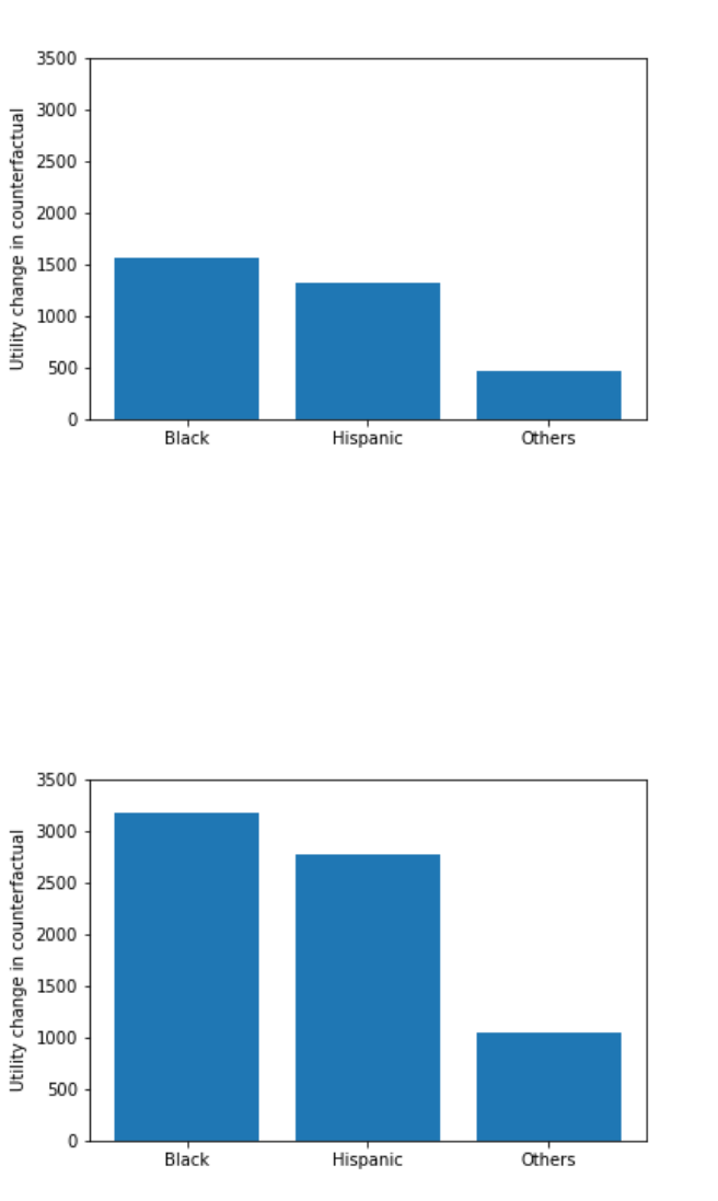
Figure A.17: Counterfactual change in utility from adding closing costs to balance of the

loan, by racial group

Note: Figure 11 plots the average diﬀerence in utility under the counterfactual contract design of adding all closing costs to the

balance of the loan. Utility is expressed in terms of the upfront dollar savings that would make borrowers indiﬀerent between

the existing system and what they would otherwise obtain in the adding closing costs to the balance of the loan counterfactual.

Figure A.18: Counterfactual change in utility from automatically reﬁnancing, by racial group

Note: Figure A.18 plots the average diﬀerence in utility under the counterfactual contract design of automatically reﬁnancing

mortgages. Utility is expressed in terms of the upfront dollar savings that would make borrowers indiﬀerent between the existing

system and what they would otherwise obtain in the adding closing costs to the balance of the loan counterfactual.