Pretest estimation in combining probability and non-probability samples

Electronic Journal of Statistics

Vol. 17 (2023) 1492–1546

ISSN: 1935-7524

https://doi.org/10.1214/23-EJS2137

Pretest estimation in combining

probability and non-probability samples

∗

Chenyin Gao and Shu Yang

Department of Statistics, North Carolina State University, Raleigh, NC 27695, USA

e-mail: [email protected]; [email protected]

Abstract: Multiple heterogeneous data sources are becoming increasingly

available for statistical analyses in the era of big data. As an important

example in ﬁnite-population inference, we develop a uniﬁed framework of

the test-and-pool approach to general parameter estimation by combining

gold-standard probability and non-probability samples. We focus on the

case when the study variable is observed in both datasets for estimating

the target parameters, and each contains other auxiliary variables. Utilizing

the probability design, we conduct a pretest procedure to determine the

comparability of the non-probability data with the probability data and

decide whether or not to leverage the non-probability data in a pooled

analysis. When the probability and non-probability data are comparable,

our approach combines both data for eﬃcient estimation. Otherwise, we

retain only the probability data for estimation. We also characterize the

asymptotic distribution of the proposed test-and-pool estimator under a

local alternative and provide a data-adaptive procedure to select the critical

tuning parameters that target the smallest mean square error of the test-

and-pool estimator. Lastly, to deal with the non-regularity of the test-and-

pool estimator, we construct a robust conﬁdence interval that has a good

ﬁnite-sample coverage property.

MSC2020 subject classiﬁcations: Primary 62D05; secondary 62E20,

62F03, 62F35.

Keywords and phrases: Data integration, dynamic borrowing, non-regularity,

Pretest estimator.

Received October 2022.

Contents

1 Introduction................................ 1493

2 Basicsetup ................................ 1495

2.1 Notation:twodatasources .................... 1495

2.2 Assumptionsandseparateestimators............... 1496

2.3 Eﬃcientestimator ......................... 1498

3 Test-and-pool estimator . . . . . . . . . . . . . . . . . . . . . . . . . 1499

3.1 Hypothesisandtest ........................ 1499

3.2 Data-driven pooling . . . . . . . . . . . . . . . . . . . . . . . . 1500

4 Asymptotic properties of the test-and-pool estimator . . . . . . . . . 1501

4.1 Asymptoticdistribution ...................... 1501

∗

Yang’s research is partially supported by the NIH 1R01AG066883 and 1R01ES031651.

1492

Test-and-pool estimator 1493

4.2 Asymptotic bias and mean squared error . . . . . . . . . . . . . 1502

4.3 Adaptiveinference ......................... 1503

5 Simulationstudy ............................. 1505

6 A real-data illustration . . . . . . . . . . . . . . . . . . . . . . . . . . 1508

7 Concludingremarks ........................... 1510

A Proofs................................... 1510

A.1 Regularityconditions........................ 1510

A.2 Proof of Lemmas 2.1 and 3.1 ................... 1512

A.3 Proof of Lemma 3.2 ........................ 1516

A.4 Proof of Theorem 4.1 ........................ 1517

A.5 Proof of the bias and mean squared error of n

1/2

(μ

tap

− μ

).. 1520

A.6 Proof of the asymptotic distribution for U(a) .......... 1522

A.7 Proof of Theorem 4.2 ........................ 1524

A.8 Proof of Remark 4.1 ........................ 1525

A.9 Proof of Lemma A.1 ........................ 1526

A.10 Proof of Lemma A.2 ........................ 1527

A.11 Proof of Lemma A.3 ........................ 1528

B Simulation................................. 1530

B.1 A detailed illustration of simulation . . . . . . . . . . . . . . . 1530

B.2 A detailed illustration of bias and mean squared error . . . . . 1536

B.3 Additionalsimulationresults ................... 1539

B.4 Double-bootstrap procedure for v

selection........... 1540

B.5 Details of the Bayesian method . . . . . . . . . . . . . . . . . . 1541

References................................... 1542

1. Introduction

It has been widely accepted that probability sampling, where each selected sam-

ple is treated as a representative sample to the target population, is the best

vehicle for ﬁnite-population inference. Since the sampling mechanism is known

based on survey design, each weight-calibrated sample can be used to obtain

consistent estimators for the target population; see [53], [15]and[24]fortext-

book discussions. However, complex and ambitious surveys are facing more and

more hurdles and concerns recently, such as costly intervention strategies and

lower participation rates. [2] address some of the current challenges in using

probability samples for ﬁnite-population inference. On the other hand, higher

demands of small area estimation and other more factors have led researchers

to seek out alternative data collection with less program budget [69, 28]. In

particular, lots of attention has been drawn to the studies of non-probability

samples.

Non-probability samples are sets of selected objects where the sampling mech-

anism is unknown. First of all, non-probability samples are readily available from

many data sources, such as satellite information [36], mobile sensor data [40],

and web survey panels [62]. In addition, these non-representative samples are

far more cost-eﬀective compared to probability samples and have the potential

1494 C. Gao and S. Yang

of providing estimates in near real-time, unlike the traditional inferences derived

from probability samples [42]. Based on these big and easy-accessible data, a

wealth of literature has been proposed which enunciates the bright future while

properly utilizing such amount of data (e.g., 18, 14, 61,and41).

However, the naive use of such data cannot ensure the statistical validity of

the resulting estimators because such non-probability samples are often selected

without sophisticated supervision. Therefore, the acquisition of large whereas

highly unrepresentative data is likely to produce erroneous conclusions. [17]and

[23] present more recent examples where non-probability samples can often lead

to estimates with signiﬁcant selection biases. To overcome these challenges, it is

essential to establish appropriate statistical tools to draw valid inferences when

integrating data from the probability and non-probability samples. Various data

integration methods have been proposed in the literature to leverage the unique

strengths of the probability and non-probability samples; see [73] for a review,

and the existing methods for data integration can be categorized into three types

including the inverse propensity score adjustment [50, 22], calibration weighting

[19, 31], and mass imputation [46, 30, 74, 11].

But most of the works assume that the non-probability sample is comparable

to the probability sample in terms of estimating the ﬁnite-population param-

eters, which may not be satisﬁed in many applications due to the unknown

sampling mechanism of the non-probability samples. Thus, the non-probability

samples with unknown sampling mechanisms may bias the estimators for the

target parameters. To resolve this issue, [47] propose a pretest to gauge the sta-

tistical adequacy of integrating the probability and non-probability samples in

an application. The pretesting procedure has been broadly practiced in econo-

metrics and medicine, and its implications are of considerable interests (e.g.,

[68, 63, 3, 72]). Essentially, the ﬁnal value of the estimator depends on the out-

come of a random testing event and therefore is a stochastic mixture of two dif-

ferent estimators. Despite the long history of the application of the pretest, few

literature investigates the theoretical properties of the underlying non-smooth

distribution for the pretest estimators.

In this paper, we establish a general statistical framework for the test-and-

pool analysis of the probability and non-probability samples by constructing a

test to gauge the comparability of the non-probability data and decide whether

or not to use non-probability data in a pooled analysis. In addition, we con-

sider the null, ﬁxed, and local alternative hypotheses for the pre-testing, rep-

resenting diﬀerent levels of comparability of the non-probability data with the

probability data. In particular, the non-probability sample is perfectly compa-

rable under the null hypothesis, whereas it is starkly incomparable under the

ﬁxed alternative. Therefore, the ﬁxed alternative cannot adequately capture the

ﬁnite-sample behavior of the pre-testing estimator, under which the test statis-

tic will diverge to inﬁnity as the sample size increases. Toward this end, we

establish the asymptotic distribution of the proposed estimator under local al-

ternatives, which provides a better approximation of the ﬁnite-sample behavior

of the pretest estimator when the idealistic assumption required for the non-

probability data is weakly violated. Also, we provide a data-adaptive procedure

Test-and-pool estimator 1495

to select the optimal values of the tuning parameters achieving the smallest

mean square error of the pretest estimator. Lastly, we construct a robust con-

ﬁdence interval accounting for the non-regularity of the estimator, which has a

valid coverage property.

The rest of the paper is organized as follows. Section 2 lays out the basic setup

and presents an eﬃcient estimator for combing the non-probability sample and

the probability sample. Section 3 proposes a test statistic and the test-and-

pool estimator. In Section 4, we present the asymptotic properties of the test-

and-pool estimator, an adaptive inference procedure, and lastly a data-adaptive

selection scheme of the tuning parameters. Section 5 presents a simulation study

to evaluate the performance of our test-and-pool estimator. Section 6 provides

a real-data illustration. All proofs are given in the Appendix.

2. Basic setup

2.1. Notation: two data sources

Let F

= {V

=(X



)



: i ∈ U} with U = {1,...,N} denote a ﬁnite

population of size N ,whereX

is a vector of covariates and Y

is the study

variable. We assume that F

is a random sample from a superpopulation model

ζ and our objective is to estimate the ﬁnite-population parameter μ

∈ R

deﬁned as the solution to



i=1

S(V

; μ)=0, (2.1)

where S(V

; μ)isal-dimensional estimating function. The class of parameters is

fairly general. For example, if S(V ; μ)=Y −μ, μ

= Y

= N

−1



i=1

is the

population mean of Y

.IfS(V ; μ)=1(Y<c)−μ for some constant c,where1(·)

is an indicator function, μ

= N

−1



i=1

1(Y

<c) is the population proportion

of Y

less than c.IfS(V ; μ)=X(Y − X



μ), μ



i=1



)

−1

(



i=1

)

is the coeﬃcient of the ﬁnite-population regression projection of Y

onto X

Suppose that there are two data sources, one from a probability sample,

referred to as Sample A, and the other from a non-probability sample, referred to

as Sample B. Assume Sample A to be independent of Sample B, and the observed

units can be envisioned as being generated through two phases of sampling [12].

Firstly, a superpopulation model ζ generates the ﬁnite population F

. Then, the

probability (or non-probability) sample is selected from it using some known (or

unknown) sampling schemes. Hence, the considered total variance of estimators

is based on the randomness induced by both the superpopulation model and

the sampling mechanisms; see Table 1 for the notations of probability order,

expectation and (co-)variance. For example, E

(·|F

) is the average over all

possible samples under the probability design for particular ﬁnite population

,andE(·) is the average over all possible samples from all possible ﬁnite

populations.

1496 C. Gao and S. Yang

Table 1

Notation and deﬁnitions.

Randomness order notation expectation (co-)variance

probability design o

(1),O

(1) E

(·|F

)var

(·|F

) , cov

(·|F

)

non-probability design o

(1),O

(1) E

(·|F

)var

(·|F

) , cov

(·|F

)

ζ model o

(1),O

(1) E

(·)var

(·) , cov

(·)

total variance o

ζ-p-np

(1),O

ζ-p-np

(1) E (·)var(·) , cov (·)

Thus far, our focus has been on the setting where the covariates X and

the study variable Y are available in both the probability and non-probability

samples, which has also been considered in [21]and[20]. The sampling indicators

are denoted by δ

A,i

and δ

B,i

, respectively; e.g., δ

A,i

= 1 if unit i is selected into

Sample A and zero otherwise. Sample A contains observations O

= {(d

−1

A,i

):i ∈A}with sample size n

,whereπ

A,i

is the known ﬁrst-order

inclusion probability for Sample A, and Sample B contains observations O

{(X

):i ∈B}with sample size n

. The unknown propensity score for being

selected into Sample B is denoted by π

B,i

. Here, A and B denote the indexes

of units in Samples A and B with total sample size n = n

+ n

and negligible

sampling fractions, i.e., n/N = o(1). Let the limits of the fractions of Sample A

and B be f

= lim

n→∞

/n and f

= lim

n→∞

/n with 0 <f

< 1.

2.2. Assumptions and separate estimators

As observing (X

) for all units i in U is usually not feasible in practice, we

can estimate the population estimating equation (2.1) by the design-weighted

sample analog under the probability sampling design



i=1

A,i

S(V

; μ)=0, (2.2)

yielding a design-weighted Z-estimator μ

[65]. When S(V ; μ) is a score function,

the resulting estimator will be a pseudo maximum likelihood estimator [58]. For

example, for estimating

,wehaveS(V ; μ)=Y − μ, which leads to μ

(



i=1

A,i

−1

A,i

)

−1



i=1

A,i

−1

A,i

. We now make the following assumption for

the design-weighted Z-estimator.

Assumption 2.1 (Design consistency and central limit theorem). Let μ

be the

corresponding design-weighted Z-estimator of μ

, which satisﬁes that var

(μ

)=O

−1

) and {var

(μ

)}

−1/2

×(μ

−μ

) |F

→N(0, 1) in distribution

as n

→∞.

Under the typical regularity conditions [24], Assumption 2.1 holds for many

common sampling designs such as probability proportional to size and stratiﬁed

simple random sampling. Under Assumption 2.1, μ

is design-consistent and

does not rely on any modeling assumptions. This explains why the probability

sampling has been the gold standard approach for ﬁnite-population inference,

and we make this assumption throughout this article.

Test-and-pool estimator 1497

Let f(Y | X) be the conditional density function of Y given X in the super-

population model ζ,andletf(X)andf(X | δ

= 1) be the density function

of X in the ﬁnite population and the non-probability sample, respectively. To

correct for the selection bias of the non-probability sample, most of the existing

literature considers the following assumptions [e.g., 46, 66, 12].

Assumption 2.2 (Common support and ignorability of sampling). (i) The vec-

tor of covariates X has a compact and convex support, with its density bounded

and bounded away from zero. Also, there exist positive constants C

and C

such

that C

≤ f(X)/f(X | δ

=1)≤ C

almost surely. (ii) Conditional on X, the

density of Y in the non-probability sample follows the superpopulation model;

i.e., f(Y | X, δ

=1)=f(Y | X). (iii) The sample inclusion indicator δ

B,i

and

B,j

are independent given X

and X

for i = j.

Assumption 2.2 (i) and (ii) constitute the strong sampling ignorability condi-

tion [50]. Assumption 2.2 (i) implies that the support of X in the non-probability

sample is the same as that in the ﬁnite population, and it can also be formulated

as a positivity assumption that P(δ

=1| X) > 0 for all X. This assumption

does not hold if certain units would never be included in the non-probability

sample. Assumption 2.2 (ii) is equivalent to the ignorability of the sampling

mechanism for the non-probability sample conditional on the covariates X, i.e.,

P(δ

=1| X, Y )=P(δ

=1| X)[34]. This assumption holds if the set of

covariates contain all the outcome predictors that aﬀect the possibility of be-

ing selected into the non-probability sample. Assumption 2.2 (iii) is a critical

condition to employ the weak law of large numbers under the non-probability

sampling design [12]. Under Assumption 2.2, the non-probability sample can be

used to produce consistent estimators. However, this assumption may be unre-

alistic if the non-probability data collection suﬀers from uncontrolled selection

biases [6], measurement errors [17], or other error-prone issues. Thus, we con-

sider Assumption 2.2 as an idealistic assumption, which may be violated and

require pretesting.

Under Assumptions 2.1 and 2.2, let Φ

(V,δ

; μ)andΦ

(V,δ

,δ

; μ)be

two l-dimensional estimating functions for the target parameter μ

when us-

ing the probability sample and the combined samples, respectively. In prac-

tice, Φ

(·)andΦ

(·) may depend on unknown nuisance functions, and solving

E{Φ

(V,δ

; μ)} =0andE{Φ

(V,δ

,δ

; μ)} = 0 is not feasible. By replacing

the nuisance functions with their estimated counterparts, and the expectations

with the empirical averages, we obtain μ

and μ

by solving



i=1



,δ

A,i

; μ)=0,



i=1



,δ

A,i

,δ

B,i

; μ)=0, (2.3)

respectively, where {



(·),



(·)} are the estimated version of {Φ

(·), Φ

(·)}.

Remark 2.1. For estimating the ﬁnite population means, that is, μ

= Y

(·) and Φ

(·) are commonly chosen as

(V,δ

; μ)=

(Y − μ), (2.4)

1498 C. Gao and S. Yang

(V,δ

,δ

; μ)=

(X)

{Y − m (X)} +

m (X) − μ, (2.5)

where π

(X)=P(δ

=1| X) and m(X)=E(Y | X, δ

=1). To obtain the

estimators μ

and μ

, parametric models π

(X; α) and m(X; β) can be posited

for the nuisance functions π

(X) and m(X), respectively.

In addition, researchers might be interested in estimating the individual-level

outcomes rather than the population-level outcomes. In this case, Φ

(·) and

(·) can be speciﬁed for estimating the outcome model m(X; β) as:

(V,δ

; β)=

∂m(X; β)

∂β

{Y − m(X; β)}

(V,δ

,δ

; β)=



(X)



∂m(X; β)

∂β

{Y − m(X; β)}.

Next, we adopt the model-design-based framework for inference, which in-

corporates the randomness over the two phases of sampling [27, 37, 7, 70]. The

asymptotic properties for μ

and μ

can be derived using the standard M-

estimation theory under suitable moment conditions.

Lemma 2.1. Suppose Assumptions 2.1, 2.2 and additional regularity condi-

tions A.1 hold. Then, we have

1/2



μ

− μ

μ

− μ



→N



l×1









, (2.6)

where V

, V

,andΓ are deﬁned explicitly in the Appendix.

In Lemma 2.1, we extend the conditional normality to unconditional as in

[55], which implies that the asymptotic (co-)variances terms V

and Γ refer

to all the sources of uncertainty over the two phases.

2.3. Eﬃcient estimator

Under Assumptions 2.1 and 2.2,bothμ

and μ

are consistent, and it is ap-

pealing to combine μ

with μ

to achieve eﬃcient estimation. We consider a

class of linear combinations of the functions in (2.3):



i=1

{



,δ

A,i

; μ)+Λ



,δ

A,i

,δ

B,i

; μ)} =0, (2.7)

where Λ is the linear coeﬃcient that gauges how much information of the non-

probability sample should be integrated with the probability sample. Equation

(2.7) leads to a class of composite estimators which is a weighted average of

μ

and μ

with Λ-indexed weight ω

and ω

.WhenΛ=0,(2.7)provides

the design-consistent estimator μ

. The optimal choice Λ

eﬀ

can be empirically

tuned to minimize the asymptotic variance of the composite estimator, leading

Test-and-pool estimator 1499

to the eﬃcient estimator μ

eﬀ

. However, the major concern for μ

eﬀ

is the possible

bias due to the violation of Assumption 2.2 (ii) for the non-probability sample.

When it is violated, it is reasonable to choose Λ = 0 and prevent any bias

associated with the non-probability sample.

3. Test-and-pool estimator

Motivated by the above reasoning, we develop a strategy that pretests the com-

parability of the non-probability sample with the probability sample ﬁrst and

then decides whether or not we should combine them for eﬃcient estimation.

We formulate the hypothesis test in Section 3.1, and construct the test-and-pool

estimator in Section 3.2.

3.1. Hypothesis and test

We formalize the null hypothesis H

when Assumption 2.2 holds, and the ﬁxed

and local alternatives H

and H

a,n

when Assumption 2.2 is violated. To be

speciﬁc, we consider

: E{Φ

(V,δ

,δ

; μ

g,0

)} =0, (3.1)

: E{Φ

(V,δ

,δ

; μ

g,0

)} = η

ﬁx

, (3.2)

a,n

: E{Φ

(V,δ

,δ

; μ

g,0

)} = n

−1/2

η, (3.3)

where μ

g,0

= E

(μ

), μ

= μ

g,0

+ O

−1/2

), and η

ﬁx

, η are two ﬁxed pa-

rameters. The ﬁxed alternative H

is commonly considered in the standard

hypothesis testing framework. However, it enforces the bias of the estimating

function Φ

(·) to be ﬁxed and indicates a strong violation of Assumption 2.2,

under which the test statistic T will diverge to inﬁnity with the sample size.

Moreover, the inference under the ﬁxed alternative can not capture the ﬁnite-

sample behavior of the test well and lacks uniform validity. On the contrary, the

local alternative provides a useful tool to study the ﬁnite-sample distribution of

non-regular estimators when the signal of violation is weak, i.e., in the n

−1/2

neighborhood of zero. In such cases, we allow the existence of a set of unmea-

sured covariates whose association with either the possibility of being selected

into Sample B or the outcome is small. Also, the local alternative H

a,n

is more

general in the sense that it reduces to H

with η = ±∞, and has been widely

employed to illustrate the non-regularity settings, such as weak instrumental

variables regression [59], regression estimators of weakly identiﬁed parameters

[13] and test errors in classiﬁcation [33]. We will mainly exploit the local alter-

native to show the inherent non-regularity of the pretest estimator.

Under the null hypothesis (3.1), μ

is consistent, and hence, it is reasonable to

combine μ

and μ

for eﬃcient estimation. However, when the null hypothesis

is violated as in (3.3), the eﬃcient estimator is biased. Lemma 3.1 presents the

asymptotic properties of the separate and eﬃcient estimators under H

a,n

1500 C. Gao and S. Yang

Lemma 3.1. Suppose Assumptions 2.1, 2.2 (i) and (iii), and all the regular-

ity conditions in Lemma 2.1 hold. Then, under the local alternative H

a,n

, the

asymptotic distributions for μ

and μ

are

1/2



μ

− μ

μ

− μ



→N



l×1

−f

−1/2

E {∂Φ

(V,δ

,δ

; μ

g,0

)/∂μ}

−1









(3.4)

The asymptotic distribution of the eﬃcient estimator μ

eﬀ

1/2

(μ

eﬀ

− μ

)→N {b

eﬀ

(η),V

eﬀ

where b

eﬀ

(η)=−f

−1/2

(Λ

eﬀ

)E {∂Φ

(V,δ

,δ

; μ

g,0

)/∂μ}

−1

η. The exact form

of ω

(Λ

eﬀ

) and V

eﬀ

are presented in Lemma A.3.

By Lemma 3.1, among the three estimators μ

, μ

and μ

eﬀ

,whenH

holds,

μ

eﬀ

is optimal because it is consistent and the most eﬃcient; while when H

violated, μ

is optimal because it is consistent but the other two estimators are

not.

We now use pretesting to guide choosing the estimators. To test H

,thekey

insight is that μ

is always consistent for μ

by Assumption 2.1,andifH

holds,



B,n

(μ

)=n

1/2

−1



i=1



,δ

A,i

,δ

B,i

; μ

) should behave as a mean-zero

random vector asymptotically. Thus, we construct the test statistic T as

T =





B,n

(μ

)





−1





B,n

(μ

)



, (3.5)

where Σ

is the asymptotic variance of Φ

B,n

(μ

, τ), and



is a consistent

estimator of Σ

. The exact form of Σ

in (A.15) involves V

, V

, and Γ. Thus,



can be obtained by replacing the unknown components in the expression of

with their estimated counterparts, and the expectations with the empirical

averages. In addition, we can consider the replication-based method for variance

estimation in Algorithm B.1 adapted from [35].

Lemma 3.2 serves as the foundation for our data-driven pooling step in Sec-

tion 3.2.

Lemma 3.2. Suppose Assumptions 2.1, 2.2 (i) and (iii), and all the regularity

conditions in Lemma 2.1 hold. Under H

, the test statistic T →χ

, i.e., a chi-

square distribution with degree of freedom l.UnderH

a,n

, T →χ

(η



−1

η/2) with

non-central parameter η



−1

η/2 as n →∞.

3.2. Data-driven pooling

If T is large, it indicates that H

may be violated and thus it is desirable to retain

only the probability sample for estimation. If T is small, it indicates that H

may

be accepted and suggests combining the probability and non-probability samples

Test-and-pool estimator 1501

for eﬃcient estimation. This strategy leads to the test-and-pool estimator μ

tap

as the solution to



i=1

{



,δ

A,i

; μ)+1(T<c

)Λ



,δ

A,i

,δ

B,i

; μ)} =0, (3.6)

where c

is the (1 − γ) critical value of χ

.In(3.6), we can ﬁx Λ to be the

optimal form Λ

eﬀ

leading to an eﬃcient estimator under H

in Section 2.3.

Alternatively, we view c

and Λ jointly as tuning parameters that determine how

much information from the non-probability sample can be borrowed in pooling.

Larger c

and Λ borrow more information from the non-probability sample,

leading to more eﬃcient but more error-prone estimators, and vice versa. We

will use a data-adaptive rule to select (Λ,c

) that minimizes the mean squared

error of μ

tap

Remark 3.1. Compare to the t-test-based pooling estimator in [38], our pro-

posed method is more general in the sense that (a) the auxiliary covariates are

used to provide a more informative model of μ

; (b) our test statistic T is mo-

tivated by the estimating function, which can be more robust to model misspec-

iﬁcation, and (c) a data-adaptive selection of (Λ,c

) is adopted for minimizing

the post-integration mean squared error.

4. Asymptotic properties of the test-and-pool estimator

In this section, we characterize the asymptotic properties of μ

tap

. Before pro-

ceeding further, we introduce more notations. Let I

l×l

be a l ×l identify matrix,

(·; η) be the cumulative distribution function for χ

with non-central param-

eter η,andF

(·)=F

(·; 0). Denote V

A-eﬀ

= V

− V

eﬀ

and V

B-eﬀ

= V

− V

eﬀ

which are both positive-deﬁnite.

4.1. Asymptotic distribution

By construction, the estimator μ

tap

is a pretest estimator that ﬁrst constructs T

for pretesting H

and then forms the test-based weights for combining μ

and

μ

. It is challenging to derive the asymptotic distribution of μ

tap

because it is

involved with the test statistic T and two asymptotically dependent components

μ

and μ

. In order to formally characterize the asymptotic distribution of

μ

tap

, we decompose the asymptotic representation of μ

tap

by two orthogonal

components, one is aﬀected by the testing and the other is not.

First, by Lemma 3.1,letn

1/2

(μ

− μ

)→Z

and n

1/2

(μ

− μ

)→Z

,where

and Z

are multivariate normal random vectors as in (3.4).

Second, by Lemma 3.2, asymptotically, we write T as a quadratic form W

with W

= −f

1/2

−1/2

E {∂Φ

(μ

g,0

,τ

)/∂μ}

−1

− Z

). We then ﬁnd an-

other standardized l-variate normal vector W

= f

1/2

−1/2

{(Γ



− V

)(Γ −

)

−1

+ Z

} that is orthogonal to W

,wherecov(W

)=0

l×l

, E(W

1502 C. Gao and S. Yang

, var(W

)=I

l×l

and E(W

)=μ

, var(W

)=I

l×l

,Σ

is introduced for the

purpose of standardization.

Third, μ

tap

can be asymptotically represented by two components involving

and W

, respectively, one component is aﬀected by the test constraint and

the other component is not. Following the above steps, Theorem 4.1 character-

izes the asymptotic distribution of μ

tap

Theorem 4.1. Suppose the assumptions in Lemma 3.1 hold except that As-

sumption 2.2 (ii) may be violated as dictated by H

a,n

in (3.3). Let W

and W

to be independent normal random vectors with mean μ

and μ

(given below,

which vary by hypothesis) and variance matrices I

l×l

. The test-and-pool estima-

tor μ

tap

follows the following asymptotic distribution

1/2

(μ

tap

− μ

)→



−V

1/2

eﬀ

+(ω

1/2

A−eﬀ

− ω

1/2

B−eﬀ

[0,c

]

w.p. ξ,

−V

1/2

eﬀ

+ V

1/2

A−eﬀ

,∞]

w.p. 1 − ξ,

where W

[a,b]

is the truncated normal distribution W

| (a ≤ W



≤ b) and

ξ = F

; μ



/2).

(a) Under H

, μ

= μ

=0,ξ = F

;0)=γ.

(b) Under H

a,n

, μ

= −Σ

−1/2

E {∂Φ

(μ

g,0

,τ

)/∂μ}

−1

η, μ

= −Σ

−1/2

η and

ξ = F

; μ

/2).

Theorem 4.1 reveals that the asymptotic distribution of μ

tap

depends on

the local parameter η and thus characterizes the non-regularity of the pretest

estimator. When H

is violated weakly (a small perturbation in the true data

generating model), the asymptotic distribution of μ

tap

can change abruptly

depending on η. The non-regularity of μ

tap

also poses challenges for inference

as shown in Section 4.3. Based on Theorem 4.1, we derive the asymptotic biases

and mean squared errors of μ

tap

under H

and H

a,n

, which serve as the stepping

stone to a data-driven procedure to select the tuning parameters Λ and c

4.2. Asymptotic bias and mean squared error

BasedontheTheorem4.1, the asymptotic distribution of μ

tap

involves elliptical

truncated normal distributions [60, 4]. To understand the asymptotic behavior

of our proposed estimator, it is crucial to comprehend the essential properties

of elliptical truncated multivariate normal distributions. We derive the moment

generating function and subsequently the mean square error of the estimator

μ

tap

. The exact form of mean squared error given by mse(Λ,c

; η)in(B.13),

albeit complicated, reveals that the amount of information borrowed from the

non-probability sample (controlled by Λ and c

) should tailor to the strength

of violation of H

(dictated by local parameter η). For illustration, we consider

a toy example in the supplemental material.

We search for the optimal values (Λ

∗

) that minimize mse(Λ,c

; η)using

standard numerical optimization algorithm [39], where η =Φ

B,n

(μ

, τ). Note

that the decision of rejecting H

or not is subject to the hypothesis testing

Test-and-pool estimator 1503

errors, namely the Type I error and Type II error. That is, the test statistic

T can be larger than c

even when H

holds; similarly, it can be small when

a,n

holds. However, the data-adaptive tuning procedure aims at minimizing

the mean squared error of the estimator μ

tap

, which implicitly restricts these

two testing errors to be small.

4.3. Adaptive inference

Standard approaches to inference, e.g., the nonparametric bootstrap, require the

estimators to be regular [56]. In non-regular settings, researchers have proposed

alternative approaches such as the m-out-n bootstrap or subsampling. However,

these approaches critically rely on a proper choice of m or the subsample size;

otherwise, the small sample performances can be poor. The non-regularity is

induced because the asymptotic distribution of the estimator μ

tap

depends on

the local parameter, thus, it does not converge uniformly over the parameter

space. [33] propose adaptive conﬁdence intervals for test errors in the classiﬁ-

cation problems. Following this idea, we construct the bound-based adaptive

conﬁdence interval (BACI) for the estimator μ

tap

that guarantees good cover-

age properties. To avoid the non-regularity, our general strategy is to derive

two smooth functionals that bound the estimator μ

tap

. Because these two func-

tionals are regular, standard approaches to inference can be adopted and valid

conﬁdence intervals follow.

To be concrete, we construct a bound-based adaptive conﬁdence interval

for a



,wherea ∈ R

is ﬁxed. By Theorem 4.1, we can reparametrize the

asymptotic distribution of a



1/2

(μ

tap

− μ

)as



1/2

(μ

tap

− μ

)→R

+ a



1/2

B-eﬀ

+ V

1/2

A-eﬀ

, (4.1)

where

= −a



1/2

eﬀ

+ a



(ω

1/2

A-eﬀ

− ω

1/2

B-eﬀ

+ a



1/2

B-eﬀ

+ V

1/2

A-eﬀ

)μ

,∞)

= W

,∞)

− μ

,∞)

and μ

,∞)

= μ



. By construction, R

is regular and asymptotically

normal, but U

is nonsmooth. Nonsmoothness and nonregularity are interre-

lated. To illustrate, if μ

=0,U

follows a standard truncated normal distribu-

tion with truncated probability P(W



≤ c

| μ

= 0); whereas, if |μ

|→∞,

P(W



≤ c

| μ

) diminishes to zero, implying that U

follows a standard

normal distribution. Thus, the limiting distribution of a



1/2

(μ

tap

− μ

)isnot

uniform over local parameter μ

(or equivalently η).

Our goal is to form the least conservative smooth upper and lower bounds.

An important observation is that if |μ

| is suﬃciently large, we may treat

as regular. Thus, we deﬁne B as the nonregular zone for μ



such that

max



∈B

P(W



≥ c

| μ

) ≤ 1 − ε for small >0andB



the regular

zone. When μ



∈ B



, standard inference can apply, and bounds are only

1504 C. Gao and S. Yang

Fig 1. Illustration of the nonregular zone B (shaded) and two power functions: the solid and

dash lines are P(W



| μ



) and P(T ≥ v

| μ



) as functions of μ



, respectively.

needed when μ



∈ B to avoid the inference procedure to be overly con-

servative. We then require another test procedure to test μ



∈ B against



∈ B



. Toward this end, we use T ≥ v

,wherev

is chosen such that

max



∈B

P(T ≥ v

| μ

)=˜α for a pre-speciﬁed ˜α. Figure 1 illustrates the

regular and nonregular zones and the test. If T ≥ ν

, we conclude the regularity

of the estimator μ

tap

and construct a normal conﬁdence interval, but if T<ν

we construct the least favorable conﬁdence interval by taking the union for all

∈ R

. In practice, v

can be determined by the double bootstrapping sat-

isfying the regularity condition that lim

n→∞

/n = 0; see Section B.4 of the

supplemental material for more details.

Accordingly, U

can be decomposed into two components U

=(W

,∞)

−

,∞)

T ≥υ

+(W

,∞)

− μ

,∞)

T<v

and only regularize (i.e., deriving

bounds for) the latter component. Continuing with (4.1), we can take the supre-

mum over all μ

in the nonregular zone to construct the upper bound U(a),

U(a)=R

+ a



1/2

B-eﬀ

+ V

1/2

A-eﬀ

)(W

,∞)

− μ

,∞)

T ≥υ

+sup

∈R





1/2

B-eﬀ

+ V

1/2

A-eﬀ

)(W

,∞)

− μ

,∞)

)



T<v

(4.2)

The lower bound L(a)fora



1/2

(μ

tap

− μ

) can be computed in an analogous

way by replacing sup with inf in (4.2). Taking the supremum and the inﬁmum

of μ

over R

renders the two bounds U(a)andL(a) smooth and regular. The

limiting distribution of U(a)is

U(a)→R + a



1/2

B-eﬀ

+ V

1/2

A-eﬀ

)(W

,∞)

− μ

,∞)



∈B



Test-and-pool estimator 1505

+sup

∈R





1/2

B-eﬀ

+ V

1/2

A-eﬀ

)(W

,∞)

− μ

,∞)

)





∈B

. (4.3)

Similarly, the limiting distribution of L(a)is(4.3) by replacing sup with inf.

Based on the limiting distribution of U(a)andL(a), if P(μ



∈ B)=0,U(a)

and L(a) have approximately the same limiting distributions as a



1/2

(μ

tap

−

). However, if P(μ



∈ B) =0,U(a) is stochastically larger and L(a)is

stochastically smaller than a



1/2

(μ

tap

− μ

Based on the regular bounds U (a)andL(a), we construct the (1 −α) ×100%

bound-based adaptive conﬁdence interval of a



BACI

,1−α

(a)=





μ

tap

−



1−α/2

(a)/

√

n, a



μ

tap

−



α/2

(a)/

√



, (4.4)

where



(a)and



(a) approximate the d-th quantiles of the distribution of U(a)

and L(a), respectively, which can be obtained by the nonparametric bootstrap

method.

Theorem 4.2. Assume the conditions in Theorem 4.1 hold true. Furthermore,

assume matrices Σ

, Σ

in Lemma 3.1 and their consistent estimates



are strictly positive-deﬁnite, and the sequence v

satisﬁes v

→∞and v

/n → 0

with probability one. The asymptotic coverage rate of (4.4) satisﬁes





∈ C

BACI

,1−α

(a)



≥ 1 − α. (4.5)

In particular, if Assumption 2.2 is strongly violated with P(μ



∈ B



)=1, the

inequality in (4.5) becomes equality.

Remark 4.1. We discuss an alternative approach to construct valid conﬁdence

intervals for the non-regular estimators using projection sets [48] (referred to as

projection-based adaptive conﬁdence intervals (PACI), C

PACI

,1−α

(a)). The basic

idea is as follows. For a given μ

, the limiting distribution of μ

tap

is known and

aregular(1 − ˜α

) × 100% conﬁdence interval C

,1− ˜α

(a; μ

) of a



can be

formed through the standard procedure. Since μ

is unknown, a (1 −α) ×100%

projection conﬁdence interval of μ

can be conservatively constructed as the

union of all C

,1− ˜α

(a; μ

) over μ

in its (1 − ˜α

) × 100% conﬁdence region,

where α =˜α

+˜α

. Such strategy may be overly conservative, and in that way, the

projection-based adaptive conﬁdence interval then introduces a pretest in order to

mitigate the conservatism. If the pretest rejects H

: μ



∈ B, C

,1− ˜α

(a; μ

)

is used; otherwise, the union of C

,1− ˜α

(a; μ

) is used. The technical details

for the C

PACI

,1−α

(a) are presented in the supplemental material. Our simulation

study later shows that the C

PACI

,1−α

(a) is more conservative than the proposed

BACI

,1−α

(a).

5. Simulation study

In this section, we evaluate the ﬁnite-sample performances of the proposed esti-

mator μ

tap

and C

BACI

,1−α

(a). First, we generate the ﬁnite population F

with size

1506 C. Gao and S. Yang

N =10

. For each subject i, generate X

=(1,X

1,i

2,i

)



,whereX

1,i

∼N(0, 1)

and X

2,i

∼N(1, 1), and generate Y

by Y

=1+X

1,i

2,i

+ε

,where

∼N(0, 1) and 

∼N(0, 1). Generate samples from the ﬁnite population F

by Bernoulli sampling with speciﬁed inclusion probabilities

log



A,i

1 − π

A,i



| X

= ν

+ .2X

1,i

+ .1X

2,i

log



B,i

1 − π

B,i



| X

= ν

+ .1X

1,i

+ .2X

2,i

+ .5n

−1/2

where ν

and ν

are adaptively chosen to ensure the target sample sizes n

≈

600 and n

≈ 5000. We assume that (X

) are observed but u

is unobserved,

and we vary b in {0, 10, 100} to represent the scenarios where H

holds, is slightly

violated or strongly violated, respectively.

We compare the estimator μ

tap

with other estimators: (a) μ

: the solu-

tion to



i=1

,δ

A,i

; μ) = 0 with Φ

,δ

A,i

; μ) deﬁned in (2.4). (b) μ

the naive sample mean



i=1

B,i

)

−1



i=1

B,i

.(c)μ

: the solution



i=1

,δ

A,i

,δ

B,i

; μ, α, β) = 0 with Φ

,δ

A,i

,δ

B,i

; μ, α, β) deﬁned in

(2.5), where (α, β) are estimated by using the maximum pseudo-likelihood es-

timator α and the ordinary least square estimator



β [26]; see Equations (B.2)

and (B.4). (d) μ

eﬀ

: the solution to (2.7) with the optimal choice Λ

eﬀ

speci-

ﬁed in (A.11) and the consistent estimators (α,



β) obtained from (c). (e) μ

eﬀ:B

μ

eﬀ

,whereα is estimated in the same manner as (c) but β is estimated solely

based on the non-probability sample; see Equation (B.3). (f) μ

eﬀ:KH

: μ

eﬀ

,where

(α, β) are estimated simultaneously by adopting the methods proposed by [29];

see Equations (B.5)and(B.6). (g) μ

tap

, μ

tap:B

, μ

tap:KH

: the solution to (3.6),

where (Λ,c

) are chosen by our data-adaptive procedure with (α,



β) obtained

from (d), (e), (f), respectively. (h) μ

Bayes:1

, μ

Bayes:2

, μ

Bayes:3

: the Bayesian ap-

proaches for combining the non-probability sample with the probability sample

assuming diﬀerent informative priors [52].

For all estimators, we specify the model π

(X; α) to be a logistic regression

model with X

and the outcome mean model m(X; β) to be a linear regression

model with X

. For non-regular estimators μ

tap

, μ

tap:B

and μ

eﬀ:KH

,wecon-

struct the C

BACI

,1−α

(a)in(4.4) with a data-adaptiv choice of ν

,theC

BACI

,1−α

(a)

with a ﬁxed v

= log log n{C

BACI:F

,1−α

(a)} (BACI

), and the C

PACI

,1−α

(a). For any

conﬁdence intervals requiring the nonparametric bootstrap, the bootstrap size

is 2000. For the Bayesian estimators, the point estimates are obtained by the

Markov chain Monte Carlo sampling with size 2000 after additional 500 burn-in

samples.

Table 2 reports the bias, variance and mean squared error of each estimator

over 2000 simulated datasets. The benchmark estimators μ

have small biases

across all scenarios, guaranteed by the probability sampling design. On the other

hand, the non-probability-only estimators

exhibit high biases in all cases,

mainly due to the eﬀect of selection bias. When the impact of the unmeasured

confounder b increases, the pooled estimators μ

eﬀ

, μ

eﬀ:B

and μ

eﬀ:KH

are be-

Test-and-pool estimator 1507

Table 2

Simulation results for bias (×10

−3

),variance(var)(×10

−3

) and mean squared error

(MSE) (×10

−3

) of μ

, μ

, μ

eﬀ

, μ

Bayes

and μ

tap

when H

holds, is slightly violated or

strongly violated.

holds slightly violated strongly violated

bias var MSE bias var MSE bias var MSE

Regular μ

−4.1 10.4 10.4 −4.1 10.4 10.4 −4.1 10.4 10.4

284.1 1.2 81.9 355.3 1.2 127.4 1318.8 2.0 1741.4

μ

−0.4 4.2 4.2 71.0 4.3 9.3 1048.0 5.0 1103.2

μ

eﬀ

−0.9 4.1 4.1 62.3 4.2 8.1 851.5 6.6 731.7

μ

eﬀ:B

−0.9 4.1 4.1 62.3 4.2 8.1 851.7 6.6 732.1

μ

eﬀ:KH

−0.9 4.1 4.1 62.3 4.2 8.1 851.5 6.7 731.7

Bayes μ

Bayes:1

−3.7 14.1 14.1 1.0 14.0 14.0 −4.3 14.1 14.1

μ

Bayes:2

−4.1 10.8 10.8 17.1 11.1 11.4 7.0 13.8 13.8

μ

Bayes:3

−2.4 8.9 8.9 51.2 9.0 11.6 614.0 10.8 387.9

TAP μ

tap

−4.8 7.6 7.6 10.1 9.3 9.4 −4.1 10.4 10.4

μ

tap:B

−4.8 7.6 7.6 10.1 9.3 9.4 −4.1 10.4 10.4

μ

tap:KH

−4.8 7.6 7.6 10.1 9.3 9.4 −4.1 10.4 10.4

Table 3

Simulation results for coverage rates (CR) (×10

−2

) and widths (×10

−3

) for 95% conﬁdence

intervals when H

holds, is slightly violated or strongly violated.

holds slightly violated strongly violated

CIs CR width CR width CR width

μ

Wald 95.2 404.1 95.3 404.1 95.2 404.0

0.0 135.5 0.0 138.8 0.0 173.7

μ

95.9 262.8 81.8 264.4 0.0 282.4

μ

eﬀ

95.9 259.5 85.1 260.9 0.0 273.6

μ

Bayes:1

hpdi 98.3 463.0 97.5 461.5 97.3 462.8

μ

Bayes:2

97.8 404.2 97.4 409.8 97.5 458.3

μ

Bayes:3

99.3 368.2 97.4 370.6 0.0 407.0

μ

tap

paci 98.4 558.7 98.4 535.7 99.2 541.0

baci

94.7 399.1 95.9 402.3 94.7 402.6

baci 92.1 363.1 93.3 367.2 94.8 402.8

coming more biased. Additionally, the Bayesian methods, particularly μ

Bayes:2

perform reasonably well when H

holds or is slightly violated, but it tends to

have large biases when H

is strongly violated. Whereas the proposed estima-

tors μ

tap

, μ

tap:B

and μ

tap:KH

have small biases regardless of the strength of the

unmeasured confounder. When H

is slightly violated, our proposed estimators

have slightly larger biases but smaller mean squared errors than μ

by inte-

grating the non-probability sample. When H

is strongly violated, the proposed

estimators perform similarly to μ

with the protection of pretesting.

Table 3 reports the properties of 95% Wald conﬁdence intervals for the regu-

lar estimators, the highest posterior density intervals (HPDIs) for the Bayesian

estimators, and various adaptive conﬁdence intervals for the non-regular es-

timators μ

tap

, where the Wald conﬁdence intervals are constructed, and the

Bayesian credible intervals are constructed based on the posterior samples after

1508 C. Gao and S. Yang

burn-in. Because the conﬁdence intervals (and the point estimates; see Table 2)

are not sensitive to the methods of estimating the nuisance parameters (α, β),

we only present the conﬁdence intervals for μ

eﬀ:KH

and μ

tap:KH

for simplicity.

BasedonTable3, C

PACI

,1−α

tend to overestimate the uncertainty, leading to

over-conservative conﬁdence intervals. C

BACI

,1−α

and C

BACI:F

,1−α

are less conserva-

tive and alleviate the over-coverage issues; thus, the empirical coverage rates are

close to the nominal level in all cases. Moreover, C

BACI

,1−α

have narrower inter-

vals than C

BACI:F

,1−α

by using the double bootstrap procedure to select v

at the

expense of computational burden. When H

holds, the C

BACI

,1−α

are narrower

than the Wald for the probability-only estimator μ

, indicating the advantages

of implementing the test-and-pool strategy in these cases. When H

is slightly

violated, the beneﬁt in coverage rate is not signiﬁcantly observed under similar

coverage rates. When H

is strongly violated, the adaptive conﬁdence interval

BACI

,1−α

reduces to the Wald conﬁdence intervals for μ

. Lastly, the credible in-

tervals for the Bayesian estimators do not have satisfactory coverage properties

as the model misspeciﬁcation persists across scenarios, which is aligned with the

Bernstein-von Mises Theorem [65, Chapter 10.2].

6. A real-data illustration

To demonstrate the practical use, we apply the proposed method to a probability

sample from the 2015 Current Population Survey (CPS) and a non-probability

sample from the 2015 Behavioral Risk Factor Surveillance System (BRFSS)

survey. Note that the Behavioral Risk Factor Surveillance System survey itself

is a probability sample and we manually discard its sampling weights to recast

it as a non-probability sample for illustrating our proposed method.

To apply the proposed method, we use a two-phase sampling survey data with

sizes n

= 1000 and n

= 8459. We focus on two outcome variables of interest:

employment (percentages of working and retired) and educational attainment

(high school or less as h.s.o.l, and college or above as c.o.a.). Both datasets

provide measurements on the outcomes of interest and some common covariates

including age, sex (female or not), race (white and black), origin (Hispanic or

not), region (northeast, south, or west), and marital status (married or not).

To illustrate the heterogeneity in the study populations, Table 4 contrasts the

means of variables from the CPS sample (design-weighted averages) and the

BRFSS sample (simple averages). Based on Table 4, the BRFSS sample may

not be representative of the target population, and the pretesting procedures

before pooling should be expected.

Table 5 presents the results. For all estimators, we specify the propensity

score model to be a logistic regression model with the covariates (all variables

excluding the outcome variable) and the outcome mean model to be a logistic

regression model with the covariates. The eﬃcient estimator μ

eﬀ

gains eﬃciency

in all estimators compared to both μ

and μ

; however, it may be subject to

biases if the non-probability sample does not satisfy the required assumptions. In

the test-and-pool analysis, the pretesting rejects the use of the non-probability

Test-and-pool estimator 1509

Table 4

The covariate means by two samples: CPS sample (a probability sample) and BRFSS

sample (a hypothetical non-probability sample.)

Data source age %sex %white %black %hispanic %northeast %south

CPS 47.5 56.5 81.9 11.0 13.3 18.1 37.7

BRFSS 48.3 54.2 83.2 8.4 8.3 20.0 27.6

%west %married %working %retired %h.s.o.l. %c.o.a.

CPS 24.1 52.5 58.7 13.6 39.4 30.3

BRFSS 29.5 50.8 52.2 24.5 21.2 41.9

Table 5

Estimated population mean (EST), standard errors (SE) and conﬁdence intervals of μ

for

selected covariates when combining two datasets.

Outcome Y %working %retire %h.s.o.l. %c.o.a.

μ

est 58.7 13.6 39.4 30.3

se 1.51 1.17 1.60 1.59

Wald (54.8,62.3) (11.6,16.2) (35.7,43.0) (27.2,33.7)

μ

est 56.5 20.0 25.8 32.3

se 1.03 1.24 0.93 1.20

Wald (54.2,58.8) (17.9,22.4) (234.0,27.5) (30.3,34.5)

μ

eﬀ:KH

est 56.6 17.3 26.4 32.1

se 0.80 0.19 0.87 0.62

Wald (54.3,58.9) (15.4,19.6) (24.6,28.1) (30.1,34.3)

μ

Bayes:1

est 59.8 14.1 40.5 30.7

se 1.97 1.37 2.00 1.84

hpdi (56.0, 63.6) (11.4,16.8) (36.6,44.4) (27.2,34.4)

μ

Bayes:2

est 59.8 14.0 40.3 30.9

se 2.01 1.33 1.92 1.84

hpdi (56.1,63.9) (11.4,16.4) (36.4,44.0) (27.2,34.5)

μ

Bayes:3

est 58.6 14.1 37.6 31.1

se 1.94 1.30 1.92 1.76

hpdi (54.7, 62.4) (11.6,16.7) (33.7,41.4) (27.7,34.7)

μ

tap:KH

est 58.7 13.6 39.0 31.7

se 1.51 1.17 1.55 0.64

baci (54.9,62.6) (11.6,15.8) (35.8,42.6) (31.0,33.6)

sample for the employment variables “working” and “retired” but accepts the use

of the non-probability sample for the education variables “high school or less”

and “college or above”. Thus, for the employment variables, μ

tap

= μ

,andfor

the educational attainment variables, μ

tap

gains eﬃciency over μ

. The Bayesian

estimators with the informative priors 2 and 3 are more eﬃcient than the prior

1. However, they still yield larger standard errors compared to the probability-

only estimator μ

perhaps because the non-probability-based informative priors

are biased for the model parameters for the probability sample. From the test-

and-pool analysis, the employment rate and the retirement rate are 58.7% and

13.6%, respectively, the percentage of the U.S. population with a high school

education or less is 39.0% and the percentage of the population with a college

education or above is 31.7% in 2015.

1510 C. Gao and S. Yang

7. Concluding remarks

When utilizing the non-probability samples, researchers often assume that the

observed covariates contain all the information needed for recovering the sam-

pling mechanism. However, this assumption may be violated, and hence the

integration of the probability and non-probability samples is subject to biases.

In this paper, we propose the test-and-pool estimator that ﬁrstly scrutinizes

the assumption required for combining by hypothesis testing and carefully com-

bines the probability and non-probability samples by a data-driven procedure to

achieve the minimum mean squared error. In theoretical development, we treat

(Λ,c

) jointly as two tuning parameters and establish the asymptotic distribu-

tion of the pretesting estimator without taking their uncertainties into account.

The non-regularity of the pretest estimator invalidates the conventional method

for generating reliable inferences. To address this issue, the proposed adaptive

conﬁdence interval has been designed to eﬀectively handle the non-smoothness

of the pretest estimator and ensure uniform validity of inferences. It is important

to note, however, that this approach may result in a little gain in the precision

of the conﬁdence interval, although the point estimator might have a signiﬁ-

cant gain in the MSE compared to the estimator based only on the probability

sample. Further research is required to develop a valid post-testing conﬁdence

interval that oﬀers reduced conservatism.

Pretest estimation is the norm rather than the exception in applied research,

so the theories that we have established are highly relevant to researchers who

engage in applied work. The proposed framework can be extended in the fol-

lowing directions. First, in this work, we study the implications of pretesting

on estimation and inference under one single pretest. In practice, researchers

may engage in multiple presetting. For example, in the data integration con-

text, one can encounter multiple data sources [51, 71, 16], requiring pretesting

of the comparability of each data source and the benchmark. Multiple preset-

ting alters the current asymptotic results and is an important future research

topic. Second, our framework considers a ﬁxed number of covariates; however,

in reality, practitioners often collect a rich set of auxiliary variables, rendering

variable selection imperative [75]. Developing a valid statistical framework to

deal with issues arising from selective inference is a challenging but important

topic for further investigation. Third, small area estimation has received a lot of

attention in the data integration context [44, 28, 25]. The typical estimator in

small area estimation is a weighted average of the design-based estimator and

a model-based synthetic estimator. [5] discussed the trade-oﬀ of the eﬃciency

gain from invoking model assumptions and the risk that these assumptions do

not hold. Thus, pretesting can be potentially useful for small-area estimation,

which we will investigate in the future.

Appendix A: Proofs

A.1. Regularity conditions

Let F

= {V

=(X



)



: i ∈ U },Φ

(V,δ

; μ)andΦ

(V,δ

,δ

; μ, τ)be

l-dimensional estimating functions for the parameter μ

∈ R

when using the

Test-and-pool estimator 1511

probability sample and the combined samples, respectively. Let Φ

(V,δ

,δ

; τ)

be the k-dimensional estimating equations for the nuisance parameter τ

∈

. Then, we construct one stacked estimating equation system Φ(V, δ

,δ

; θ)

with θ =(μ



,μ



,τ



)



and dim(θ)=2l + k. For establishing our stochastic

statements, we require the following regularity conditions.

Assumption A.1. The following regularity conditions hold.

a) The parameter θ =(μ



,μ



,τ



)



belongs to a compact parameter spaces

Θ in R

2l+k

b) There exist a unique solution θ

=(μ



A,0

,μ



B,0

,τ



)



lying in the interior

of the compact space Θ such that

E{Φ

(V,δ

; θ

)} = E{Φ

(V,δ

,δ

; θ

)} = E{Φ

(V,δ

,δ

; θ

)} =0.

c) Φ(V,δ

,δ

; θ) is integrable with respect to the joint distribution of (V , δ

) for all θ in a neighborhood of θ

d) The ﬁrst two partial derivatives of E{Φ(V,δ

,δ

; θ)} and their empirical

estimators are invertible for all θ in a neighborhood of θ

e) For all j, k, l ∈{1, ···, 2l +k}, there is an integrable function B(V,δ

,δ

)

such that

|∂Φ

(V,δ

,δ

; θ)/∂θ

∂θ

|≤B(V,δ

,δ

), E {B(V,δ

,δ

)} < ∞,

for all θ in a neighborhood of θ

almost surely.

f) {V

: i ∈U}are a set of i.i.d. random variables s.t. E{|Φ(V,δ

,δ

; θ)|

2+δ

}

is uniformly bounded for θ in a neighborhood of θ

g) The sample sizes n

and n

are in the same order of magnitude, i.e., n

O(n

). The sampling fractions for both Sample A and B are negligible, i.e.,

n/N = o(1),wheren = n

+ n

h) There exist C

and C

such that 0 <C

≤ Nπ

A,i

≤ C

and 0 <C

≤

Nπ

B,i

≤ C

for all i ∈U.

Assumption A.1 a)-e) are typical ﬁnite moment conditions to ensure the

consistency of the solution to the estimating functions [49, Appendix B], [64,

Section 3.2], [9, page 293] and [67, Appendix C]. Assumption A.1 f) is required

for obtaining the asymptotic normality of μ

under superpopulation. Assump-

tion A.1 g) states that the sampling fraction is negligible, which is helpful

for subsequent variance estimation, and we can use O(n

−1/2

), O(n

−1/2

)and

O(n

−1/2

) interchangeably. Assumption A.1 h) implies that the inclusion prob-

abilities for Samples A and B are in the order of n/N , which is necessary to

establish their root-n consistency.

It is noteworthy that in Assumption 2.1, the asymptotic normality is as-

certained for the design-weighted estimators given the ﬁnite population F

Hereby, we extend the conditional normality to the unconditional one, which

averages over all possible ﬁnite populations satisfying the Assumption A.1 (f).

The following lemma plays a key role to establish the stochastic statements [24,

Theorem 1.3.6.].

1512 C. Gao and S. Yang

Lemma A.1. Under Assumption 2.1 and Assumption A.1 (f), let {F

} be

a sequence of ﬁnite populations and A

be a sample selected from the Nth

population by PR design with size n

. Assume that

lim

N→∞

= ∞, lim

N→∞

N − n

= ∞.

We know that the distribution of the design-weighted estimator μ

and ﬁnite-

population estimator μ

are both asymptotically normal distributed such that

μ

∼N(μ

),μ

∼N(μ

g,0

where

∼ denotes the asymptotic distribution. Then, μ

−μ

is also asymptotically

normal.

By lemma A.1, the sampling fraction is negligible, and therefore the limiting

variance of lim

N→∞

1/2

(μ

− μ

g,0

) is 0, indicating that the intermediate step

of producing the ﬁnite population is of little signiﬁcance.

A.2. Proof of Lemmas 2.1 and 3.1

In the general case, we begin to investigate the statistical properties of

A,n

(μ

, τ)=n

1/2

−1



i=1

,δ

A,i

; μ

, τ)

and

B,n

(μ

, τ)=n

1/2

−1



i=1

,δ

A,i

,δ

B,i

; μ

, τ).

First, to simplify our notations, let

(V,δ

; μ, τ)=∂Φ

(V,δ

; μ, τ)/∂μ,

(V,δ

,δ

; μ, τ)=∂Φ

(V,δ

,δ

; μ, τ)/∂μ,

B,τ

(V,δ

,δ

; μ, τ)=∂Φ

(V,δ

,δ

; μ, τ)/∂τ,

(V,δ

,δ

; τ)=∂Φ

(V,δ

,δ

; τ)/∂τ.

By the Taylor expansion of Φ

B,n

(μ

, τ)at(μ

,τ

), we have

0=Φ

B,n

(μ

, τ)

= n

1/2

−1



i=1

,δ

A,i

,δ

B,i

; μ

,τ

)

1/2

−1



i=1

B,τ

,δ

A,i

,δ

B,i

; μ

∗

, τ

∗

)(τ − τ

)

Test-and-pool estimator 1513

1/2

−1



i=1

,δ

A,i

,δ

B,i

; μ

∗

, τ

∗

)(μ

− μ

), (A.1)

for some (μ

∗

, τ

∗

) lying between (μ

, τ)and(μ

,τ

), which leads to

− n

1/2

−1



i=1

; μ

∗

, τ

∗

)(μ

− μ

) (A.2)

= n

1/2

−1



i=1

,δ

A,i

,δ

B,i

; μ

,τ

)

+ n

1/2

−1



i=1

B,τ

,δ

A,i

,δ

B,i

; μ

∗

, τ

∗

)(τ − τ

Also, under Assumption A.1 a), b) and c), by the Taylor expansion, we have

1/2

(τ − τ

)=−





i=1

; τ

)



−1



1/2

−1



i=1

,δ

A,i

,δ

B,i

; τ

)



+ o

ζ-p-np

(1), (A.3)

as τ → τ

. Also, under Assumption A.1 (e), we know that

−1



i=1

; μ

∗

, τ

∗

) → E{

(V ; μ

g,0

,τ

)},

−1



i=1

; τ

) → E {φ

(V ; τ

)},

−1



i=1

; μ

∗

, τ

∗

) → E{

(V ; μ

g,0

,τ

)},

−1



i=1

B,τ

; μ

∗

, τ

∗

) → E {φ

B,τ

(V ; μ

g,0

,τ

)},

(A.4)

where the ﬁrst two probability convergence can be straightforward to obtain by

Weak Law of Large Numbers under Assumption A.1 f) and continuous map-

ping theorem as μ

→ μ

g,0

,(μ

, τ) → (μ

g,0

,τ

) by design and (μ

∗

, τ

∗

)islying

between (μ

, τ)and(μ

g,0

,τ

). As for the third and fourth probability conver-

gence, we ﬁrst prove that μ

B,0

− μ

g,0

= o

np-p-ζ

(1) under the local alternative

E{Φ

(V,δ

,δ

; μ

g,0

,τ

)} = n

−1/2

η in Lemma A.2.

Lemma A.2. Under Assumptions 2.1, 2.2 (iii) and suitable moments condi-

tions in Assumption A.1, we have μ

B,0

− μ

g,0

= O

np-p-ζ

−1/2

1514 C. Gao and S. Yang

Next, we have under Assumption A.1 e),

−1



i=1

; μ

∗

, τ

∗

)

∼

−1



i=1

; μ

g,0

,τ

)+N

−1



i=1

∂

; μ

,τ

)

∂μ∂μ



(μ

∗

− μ

g,0

)

∼

−1



i=1

; μ

g,0

,τ

)+O

ζ-p-np

{(μ

∗

− μ

B,0

)+(μ

B,0

− μ

g,0

)}

= E{

(V ; μ

g,0

,τ

)} + o

ζ-p-np

(1),

(A.5)

where A

∼

means that A

= B

+ o

ζ-p-np

(1) and μ

lies between μ

∗

and

g,0

.Sinceμ

→ μ

B,0

,μ

→ μ

g,0

and μ

∗

lies between μ

and μ

, we establish

the second approximation in (A.5)as

(μ

∗

− μ

B,0

)+(μ

B,0

− μ

g,0

)=O

−1/2

)+O

−1/2

)=o

ζ-p-np

(1),

since n

/N = o(1). The probability convergence of N

−1



i=1

B,τ

; μ

∗

, τ

∗

)

can be established similarly and hence we obtain the last two parts of (A.4). By

plugging (A.3)and(A.4)into(A.2), we obtain the inﬂuence function for μ

1/2

(μ

− μ

)

∼

−E



(V ; μ

g,0

,τ

)



−1



1/2

−1



i=1

,δ

A,i

,δ

B,i

; μ

,τ

)

−E {φ

B,r

(V ; μ

g,0

,τ

)}·E {φ

(V ; τ

)}

−1



1/2

−1



i=1

,δ

A,i

,δ

B,i

; τ

)



∼

1/2

−1



i=1

; μ

,τ

), (A.6)

where ψ

; μ, τ) is the inﬂuence function for estimation of μ

under H

.For

completeness, we deﬁne the inﬂuence function ψ

; μ, τ) for estimator μ

an analogous way as

1/2

(μ

− μ

)

∼

−n

1/2

−1



i=1



−1



i=1

,δ

A,i

; μ

∗

, τ

∗

)



−1

×{Φ

,δ

A,i

; μ

,τ

)+φ

A,τ

; μ

∗

, τ

∗

) · (τ − τ

)} (A.7)

∼

−E



(V ; μ

g,0

,τ

)



−1



1/2

−1



i=1

,δ

A,i

; μ

,τ

)

−E {φ

A,τ

(V ; μ

g,0

,τ

)}·E {φ

(V ; τ

)}

−1



1/2

−1



i=1

,δ

A,i

,δ

B,i

; τ

)



Test-and-pool estimator 1515

∼

1/2

−1



i=1

; μ

,τ

), (A.8)

where φ

A,r

(V ; μ, τ)=∂Φ

(V,δ

; μ, τ)/∂τ . By Lemma A.1, the joint asymptotic

distribution for n

1/2

(μ

− μ

)andn

1/2

(μ

− μ

) would be

1/2



μ

− μ

μ

− μ



→



l×1

−f

−1/2

[E {∂Φ

; μ

g,0

,τ

)/∂μ}]

−1









where V

, ΓandV

are the total (co-)variance of two-phase design averaging

over the ﬁnite populations:

= nN

−2



var





i=1

; μ

,τ

) |F



+ nN

−2

var







i=1

; μ

,τ

) |F



= nN

−2



var

p-np





i=1

; μ

,τ

) |F



+ nN

−2

var



p-np





i=1

; μ

,τ

) |F



Γ=nN

−2



cov

p-np





i=1

; μ

,τ



i=1

; μ

,τ

) |F



+ nN

−2

× var







i=1

; μ

,τ

) |F



, E

p-np





i=1

; μ

,τ

) |F



where the ﬁrst term is attributed to the randomness of probability (and non-

probability) sample designs, and the second term is attributed to the random-

ness of the superpopulation model. The rest of the proof is summarized in

Lemma A.3.

Lemma A.3. Under the Assumption A.1 and the asymptotic joint distribution

for μ

and μ

in Lemma 3.1, the form of μ

eﬀ

which maximizes the variance

reduction under H

would be

1/2

(μ

eﬀ

− μ

)

∼

1/2

{ω

(Λ

eﬀ

)(μ

− μ

)+ω

(Λ

eﬀ

)(μ

− μ

)},

where the weight functions are

(Λ) = E



A,B,n

(Λ,μ

g,0

,τ

)



−1



,δ

A,i

; μ

g,0

,τ

)



, (A.9)

1516 C. Gao and S. Yang

(Λ) = E



A,B,n

(Λ,μ

g,0

,τ

)



−1

ΛE



,δ

A,i

,δ

B,i

; μ

g,0

,τ

)



, (A.10)

where

A,B,n

(Λ,μ

g,0

,τ

,δ

A,i

; μ

g,0

,τ

)+Λ

,δ

A,i

,δ

B,i

; μ

g,0

,τ

The most eﬃcient estimator μ

eﬀ

with

eﬀ

= E



; μ

g,0

,τ

)



− Γ)(V

− Γ



)

−1



; μ

g,0

,τ

)



−1

(A.11)

has the asymptotic distribution under H

a,n

1/2

(μ

eﬀ

− μ

) →N{b

eﬀ

(η),V

eﬀ

where b

eﬀ

(η)=−f

−1/2

(Λ

eﬀ

) {E∂Φ

(μ

g,0

,τ

)/∂μ}

−1

η and

eﬀ





(Λ

eﬀ

)



(Λ

eﬀ

)











(Λ

eﬀ

)

(Λ

eﬀ

)



When μ

and μ

are both scalar, V

eﬀ

would reduce to

eﬀ

=(V

− Γ

)(V

+ V

− 2Γ)

−1

= V

− V

where V

=(V

− Γ)

+ V

− 2Γ)

−1

A.3. Proof of Lemma 3.2

By applying the Taylor expansion with Lagrange forms of remainder to the

asymptotic distribution for n

1/2

−1



i=1

,δ

A,i

,δ

B,i

; μ

, τ)in(3.5) could

be shown as

1/2

−1



i=1

,δ

A,i

,δ

B,i

; μ

, τ)=n

1/2

−1



i=1

,δ

A,i

,δ

B,i

; μ

,τ

)

+ n

1/2

−1



i=1



∂Φ

,δ

A,i

,δ

B,i

;μ

∗

,τ

∗

)

∂μ

∂Φ

,δ

A,i

,δ

B,i

;μ

∗

,τ

∗

)

∂τ





μ

− μ

τ − τ



where (μ

∗

)



is the neighborhood of (μ

g,0

,τ

)



as plimμ

= μ

g,0

and

plimτ = τ

. Under the Assumption A.1 e), we have

1/2

−1



i=1

,δ

A,i

,δ

B,i

; μ

, τ)

= n

1/2

−1



i=1

,δ

A,i

,δ

B,i

; μ

,τ

) (A.12)

+ n

1/2

−1



i=1

∂Φ

B,j

,δ

A,i

,δ

B,i

; μ

∗

,τ

∗

)

∂μ

(μ

− μ

)

+ n

1/2

−1



i=1

∂Φ

,δ

A,i

,δ

B,i

; μ

∗

,τ

∗

)

∂τ

(τ − τ

)

Test-and-pool estimator 1517

= n

1/2

−1



i=1

,δ

A,i

,δ

B,i

; μ

,τ

)

+ E



∂Φ

(V,δ

,δ

; μ

g,0

,τ

)

∂τ



1/2

(τ − τ

) (A.13)

+ E



∂Φ

(V,δ

,δ

; μ

g,0

,τ

)

∂μ



1/2

(μ

− μ

)+o

ζ-p-np

(1).

Next, by replacing the ﬁrst two term in Equation (A.13) with Equation (A.2),

we have

1/2

−1



i=1

,δ

A,i

,δ

B,i

; μ

, τ)

= −E



∂Φ

(V,δ

,δ

; μ

g,0

,τ

)

∂μ



1/2

(μ

− μ

)

+ E



∂Φ

(V,δ

,δ

; μ

g,0

,τ

)

∂μ



1/2

(μ

− μ

)+o

ζ-p-np

(1)

= −(n

/n)

1/2

· E

; μ

g,0

,τ

) · n

1/2

(μ

− μ

)

+(n

/n)

1/2

· E

; μ

g,0

,τ

) · n

1/2

(μ

− μ

)+o

ζ-p-np

(1),

provided by WLLN under Assumptions 2.1, 2.2 (iii) and Assumption A.1.By

the joint distribution of μ

and μ

in Lemma 3.1, the variance of Φ

B,n

(μ

, τ)

would be

= f



; μ

g,0

,τ)



+ V

− Γ



− Γ)



; μ

g,0

,τ)





Thus, the asymptotic distribution for Φ

B,n

,δ

A,i

,δ

B,i

; μ

, τ) would be

1/2

−1



i=1

,δ

A,i

,δ

B,i

; μ

, τ)

→N



η, f



; μ

g,0

,τ)



+ V

− Γ



− Γ)



; μ

g,0

,τ)







A.4. Proof of Theorem 4.1

From Lemma 2.1 and 3.1, we know that the asymptotic joint distribution for

μ

and μ

would be

1/2



μ

− μ

μ

− μ



→N



l×1

−f

−1/2

[E {∂Φ

(μ

g,0

,τ

)/∂μ}]

−1









For simplicity, we let n

1/2

(μ

− μ

)andn

1/2

(μ

− μ

) be asymptotically dis-

tributed as Z

and Z

, respectively. Then, Φ

B,n

,δ

A,i

,δ

B,i

; μ

, τ) could be

1518 C. Gao and S. Yang

expressed as

1/2

−1



i=1

,δ

A,i

,δ

B,i

; μ

, τ)

∼

− n

1/2

−1



i=1

,δ

A,i

,δ

B,i

; μ

g,0

,τ

)(μ

− μ

)

+ n

1/2

−1



i=1

,δ

A,i

,δ

B,i

; μ

g,0

,τ

)(μ

− μ

)

→f

1/2



(V,δ

,δ

; μ

g,0

,τ

)



− Z

Let U

= f

1/2



(V,δ

,δ

; μ

g,0

,τ

)



−Z

). Next step, we attempt to ﬁnd

another linear combination of Z

and Z

which is orthogonal to U

. Observed

that when U

= f

1/2

{(Γ



−V

)(Γ −V

)

−1

+ Z

}, it is easy to verify that the

covariance of U

and U

is zero under H

cov(U

)=f



(V,δ

,δ

; μ

g,0

,τ

)





l×l

−I

l×l













(Γ



− V

)

−1

(Γ − V

)

l×l



= f



(V,δ

,δ

; μ

g,0

,τ

)



× (

− Γ



Γ − V

) ×



(Γ



− V

)

−1

(Γ − V

)

l×l



l×l

Also, since U

and U

are both asymptotically normal distributions, which im-

plies that zero covariance leads to independency. After a few standardization

procedures, we have W

and W

as W

=Σ

−1/2

, W

=Σ

−1/2

with Σ

and Σ

deﬁned as

=var(U

)=f

var{(Γ



− V

)(Γ − V

)

−1

+ Z

}, (A.14)

= f



(μ

g,0

,τ

)



+ V

− Γ



− Γ)



(μ

g,0

,τ

)





. (A.15)

Therefore, we have the form for the standardized random variables W

and W

=Σ

−1/2

= f

1/2

−1/2

{(Γ



− V

)(Γ − V

)

−1

+ Z

= −Σ

−1/2

= −(V

+ V

− Γ



− Γ)

−1/2

− Z

Here we use −Σ

−1/2

to standardize U

for the sake of convenience later. There-

fore, under the local alternative H

a,n

: E{Φ

(V,δ

,δ

; μ

g,0

,τ

)} = n

−1/2

η,

we have that E(Z

)=0, E(Z

)=−f

−1/2



(μ

g,0

,τ

)



−1

η. Combining the

above leads to

∼ N(μ

l×l

),W

∼ N(μ

l×l

Test-and-pool estimator 1519

where

= −Σ

−1/2



(μ

g,0

,τ

)



−1

η,

= −f

−1/2

+ V

− Γ



− Γ)

−1/2



(μ

g,0

,τ

)



−1

η = −Σ

−1/2

η,

and since W

⊥ W

, we could project out TAP estimator μ

tap

with the opti-

mal tuning parameter (Λ

∗

) onto these two basis respectively. First, on the

condition that

T>c

∗

= {Φ

B,n

(μ

, τ)}



−1

{Φ

B,n

(μ

, τ)} >c

∗

→W



∗

we have

1/2

(μ

tap

− μ

) | T>c

∗

= n

1/2

(μ

− μ

) | T>c

∗

→Z



∗

→−f

−1/2

(Γ − V

)(V

+ V

− Γ



− Γ)

−1

+ f

−1/2

(Γ − V

)(V

+ V

− Γ



− Γ)

−1



(μ

g,0

,τ

)



−1



∗

→−f

−1/2

+ V

− Γ



− Γ)

−1

1/2

+(Γ− V

)(V

+ V

− Γ − Γ



)

−1/2



∗

→−V

1/2

eﬀ

+ V

1/2

A-eﬀ



∗

Next, on the condition T = W



≤ c

∗

,wehave

1/2

(μ

tap

− μ

)→ω

∗

+ ω

∗



≤ c

∗

→−f

−1/2

(Γ − V

)(V

+ V

− Γ



− Γ)

−1

+ f

−1/2

∗

(Γ − V

)(V

+ V

− Γ



− Γ)

−1



(μ

g,0

,τ

)



−1

| W



≤ c

∗

− f

−1/2

∗

(Γ



− V

)(V

+ V

− Γ



− Γ)

−1



(μ

g,0

,τ

)



−1

| W



≤ c

∗

→−f

−1/2

+ V

− Γ



− Γ)

−1

1/2

+ f

−1/2

∗

(Γ − V

)(V

+ V

− Γ − Γ



)

−1/2

| W



≤ c

∗

− f

−1/2

∗

(Γ



− V

)(V

+ V

− Γ



− Γ)

−1/2

| W



≤ c

∗

→−V

1/2

eﬀ

+(ω

1/2

A-eﬀ

− ω

1/2

B-eﬀ



≤ c

∗

where W

= W



≤ c

,andω

∗

,ω

∗

are the new tuned weighted functions

deﬁned in (A.9)and(A.10) with Λ = Λ

∗

. In this way, we could fully characterize

the asymptotic distribution for the TAP estimator μ

tap

under the optimal tuning

parameter as,

1/2

(μ

tap

− μ

)→



−V

1/2

eﬀ

+(ω

1/2

A-eﬀ

− ω

1/2

B-eﬀ

[0,c

]

w.p. ξ,

−V

1/2

eﬀ

+ V

1/2

A-eﬀ

∗

,∞]

w.p. 1 − ξ,

where ξ = P(W



∗

1520 C. Gao and S. Yang

A.5. Proof of the bias and mean squared error of n

1/2

(



tap

− μ

)

For general case, given W

∼ N

(μ

p×p

), the MGF of truncated normal dis-

tribution W

|a ≤ W



≤ b is [60]

αm(t)=E{exp(t



)}

=(2π)

−p/2



exp(t



)exp



−

− μ

)



− μ

)



=(2π)

−p/2

exp(



t + μ





exp



−

− μ

− t)



− μ

− t)



=exp(−



)

∞



k=0

p+2k

(b) − F

p+2k

(a)}{(μ

+ t)



(μ

+ t)/2}

/k!,

where α = F

(b; μ



/2) − F

(a; μ



/2) is the normalization constant and

(a; μ



/2) is CDF of chi-square distribution at value a with non-central

parameter μ



/2. The second and the third equality above are justiﬁed by

(2π)

−p/2



exp



−

− μ

− t)



− μ

− t)



= P{a ≤ W



≤ b | W

∼N(μ

+ t, I

p×p

)}

= F {b; k = p, λ =(μ

+ t)



(μ

+ t)}−F {a; k = p, λ =(μ

+ t)



(μ

+ t)}

=exp{−

(μ

+ t)



(μ

+ t)}

∞



k=0

p+2k

(b) −F

p+2k

(a)}{(μ

+ t)



(μ

+ t)/2}

/k!.

To compute the ﬁrst and second moment of this truncated normal distribution,

we take derivative of the MGF and evaluate the function at t =0

dm(t)





t=0

=(μ

+ t)exp(−



)

∞



k=0

p+2k+2

(b) −F

p+2k+2

(a)}{(μ

+ t)



(μ

+ t)}/k!|

t=0

= μ

exp(−



)

∞



k=0

p+2k+2

(b) − F

p+2k+2

(a)}{μ



/2}

/k!

= μ

p+2

(b; μ



/2) − F

p+2

(a; μ



/2)}.

By the nature of MGF, we obtain the expectation of the ﬁrst moment of W

E(W

|a ≤ W



≤ b)=μ

p+2

(b; μ



/2) − F

p+2

(a; μ



/2)

(b; μ



/2) − F

(a; μ



/2)

Test-and-pool estimator 1521

Then, taking the second derivative of the MGF follows by

m(t)

dtdt





t=0

=exp(−



)



∞



k=0

p+2k+2

(b) −F

p+2k+2

(a)}{(μ

+ t)



(μ

+ t)/2}

/k!|

t=0

+(μ

+ t)(μ

+ t)



∞



k=0

p+2k+4

(b) −F

p+2k+4

(a)}{(μ

+ t)



(μ

+ t)/2}

/k!|

t=0



=exp(−



)



∞



k=0

p+2k+2

(b) −F

p+2k+2

(a)}{μ



/2}

/k!

+μ



∞



k=0

p+2k+4

(b) −F

p+2k+4

(a)}{μ



/2}

/k!



= I

p×p

p+2

(b; μ



/2) − F

p+2

(a; μ



/2))

+ μ



p+4

(b; μ



/2) − F

p+4

(a; μ



/2)),

which leads to

E(W

|a ≤ W

≤ b)=I

p×p

p+2

(b; μ

/2) − F

p+2

(a; μ

/2)

(b; μ

/2) − F

(a; μ

/2)

+ μ



p+4

(b; μ

/2) − F

p+4

(a; μ

/2)

(b; μ

/2) − F

(a; μ

/2)

In our case,

p = l, μ

= −Σ

−1/2

[E {∂Φ

(μ

g,0

,τ

)/∂μ}]

−1

η, μ

= −Σ

−1/2

η.

Recall, for T ≤ c

,wehaven

1/2

(μ

tap

−μ

)→−V

1/2

eﬀ

+(ω

1/2

A-eﬀ

−ω

1/2

B-eﬀ



≤ c

with probability ξ = F

; μ



), the bias would be

bias(λ, c

; η)

T ≤c

= −V

1/2

eﬀ

+(ω

1/2

A-eﬀ

− ω

1/2

B-eﬀ

) · E(W



≤ c

)

= −V

1/2

eﬀ

+(ω

1/2

A-eﬀ

− ω

1/2

B-eﬀ

) ·

l+2

; μ

/2)μ

; μ

/2)

The MSE can be derived based on the known formula mse(X + Y )=var(X +

Y )+{E(X + Y )}

⊗2

= {var(X)+μ

⊗2

} + {var(Y )+μ

⊗2

} +2μ



mse(λ, c

; η)

T ≤c

= V

1/2

eﬀ

(μ



+ I

l×l

1/2

eﬀ

+(ω

1/2

A-eﬀ

− ω

1/2

B-eﬀ

)

× E(W



≤ c

)(ω

1/2

A-eﬀ

− ω

1/2

B-eﬀ

)

− 2V

1/2

eﬀ

E(W



≤ c

)(ω

1/2

A-eﬀ

− ω

1/2

B-eﬀ

)

= V

1/2

eﬀ

(μ



+ I

l×l

1/2

eﬀ

+(ω

1/2

A-eﬀ

− ω

1/2

B-eﬀ

)

1522 C. Gao and S. Yang



l+2

; μ

/2)

; μ

/2)

l×l

l+4

; μ

/2)

; μ

/2)





(ω

1/2

A-eﬀ

− ω

1/2

B-eﬀ

)

−

l+2

; μ

/2)

; μ

/2)

1/2

eﬀ



(ω

1/2

A-eﬀ

− ω

1/2

B-eﬀ

For T>c

,wehaven

1/2

(μ

tap

− μ

)→−V

1/2

eﬀ

+ V

1/2

A-eﬀ



with

probability 1 −ξ =1−F

; μ



), the corresponding bias and MSE would be

bias(λ, c

; η)

T>c

= −V

1/2

eﬀ

+ V

1/2

A-eﬀ

· E(W



)

= −V

1/2

eﬀ

+ V

1/2

A-eﬀ

1 − F

l+2

; μ

/2)μ

1 − F

; μ

/2)

and

mse(λ, c

; η)

T>c

= V

1/2

eﬀ

(μ



+ I

l×l

1/2

eﬀ

+ V

1/2

A-eﬀ

E(W



1/2

A-eﬀ

− 2V

1/2

eﬀ

E(W



1/2

A-eﬀ

= V

1/2

eﬀ

(μ



+ I

l×l

1/2

eﬀ

+ V

1/2

A-eﬀ



1 − F

l+2

; μ

/2)

1 − F

; μ

/2)

l×l

1 − F

l+4

; μ

/2)

1 − F

; μ

/2)





1/2

A-eﬀ

− 2



1 − F

; μ

/2)

1 − F

; μ

/2)



1/2

eﬀ



1/2

A-eﬀ

Overall, the bias and mean squared error for n

1/2

(μ

tap

−μ

) can be characterized

bias(λ, c

; η)=ξ ·bias(λ, c

; η)

T ≤c

+(1− ξ) · bias(λ, c

; η)

T>c

mse(λ, c

; η)=ξ ·mse(λ, c

; η)

T ≤c

+(1− ξ) · mse(λ, c

; η)

T>c

A.6. Proof of the asymptotic distribution for U (a)

Throughout the proof, we assume that the regularity conditions in Lemma 2.1

and assumptions in Theorem 4.2 hold, we prove that the coverage probability

for the adaptive projection sets is guaranteed to be larger than 1 − α,whichis





∈ C

BACI

,1−α

(a)



≥ 1 − α + o(1),

where C

BACI

,1−α

(a)=





μ

tap

−



1−α/2

(a)/

√

n, a



μ

tap

−



α/2

(a)/

√



. As we al-

ready know that



1/2

(μ

tap

− μ

) ≤ U(a),a



1/2

(μ

tap

− μ

) ≥ L(a),

it is needed to show that



U(a) obtained by bootstrapping converges to the same

asymptotic distribution as U(a). Let D

p×p

denotes the space of p ×p symmetric

Test-and-pool estimator 1523

positive-deﬁnite matrices equipped with the spectral norm. We can rewrite U(a)

U(a)=−a



1/2

eﬀ

{Σ

1/2

(μ

− μ

),n

1/2

(μ

− μ

),τ}

+ a



(ω

1/2

A-eﬀ

− ω

1/2

B-eﬀ

{Σ

1/2

(μ

− μ

),n

1/2

(μ

− μ

),τ}

+ a



1/2

B-eﬀ

+ V

1/2

A-eﬀ

)μ

,∞)

+ a



1/2

B-eﬀ

+ V

1/2

A-eﬀ

)



{Σ

1/2

(μ

− μ

),n

1/2

(μ

− μ

),τ}

,∞)

− μ

,∞)



T ≥υ

+ a



1/2

B-eﬀ

+ V

1/2

A-eﬀ

)

× sup

∈R



{Σ

1/2

(μ

− μ

),n

1/2

(μ

− μ

),τ}

,∞)

− μ

,∞)



T<υ

Next, we adopt the notation for the bootstrapping to express the upper bound



U(a)=U

(b)

(a)as

(b)

(a)=−a



1/2

eﬀ

{



1/2

(μ

(b)

− μ

),n

1/2

(μ

(b)

− μ

), τ}

+ a



(ω



1/2

A-eﬀ

− ω



1/2

B-eﬀ

{



1/2

(μ

(b)

− μ

),n

1/2

(μ

(b)

− μ

), τ}

+ a



(



1/2

B-eﬀ



1/2

A-eﬀ

)

(b)

,∞)

+ a



(



1/2

B-eﬀ



1/2

A-eﬀ

)



{



1/2

(μ

(b)

− μ

),n

1/2

(μ

(b)

− μ

), τ}

,∞)

−

(b)

,∞)



T ≥υ

+ a



(



1/2

B-eﬀ



1/2

A-eﬀ

)

× sup

∈R



{



1/2

(μ

(b)

− μ

),n

1/2

(μ

(b)

− μ

), τ}

,∞)

− μ

,∞)



T<υ

where

(b)

=(1/K)



b=1

{



1/2

(μ

(b)

−μ

),n

1/2

(μ

(b)

−μ

), τ}.Next,we

deﬁne some functions to proceed our proof. w

: D

l×l

×D

l×l

×R

×R →

R, w

: D

l×l

×R

→ R and ρ : D

2l×2l

×D

l×l

×R

×R×R

→

R are functions deﬁned as below

(Σ

, Σ

, G

,τ,μ

)=−a



1/2

eﬀ

(Σ

, G

,τ)

+ a



(ω

1/2

A-eﬀ

− ω

1/2

B-eﬀ

(Σ

, G

,τ)

+ a



1/2

B-eﬀ

+ V

1/2

A-eﬀ

)μ

,∞)

+ a



1/2

B-eﬀ

+ V

1/2

A-eﬀ

)



(Σ

, G

,τ)

,∞)

− μ

,∞)





∈B



(Σ

, G

,μ

)=a



1/2

B-eﬀ

+ V

1/2

A-eﬀ

)



(Σ

, G

,τ)

,∞)

− μ

,∞)





∈B,

(Σ

, G

,μ

)=a



1/2

B-eﬀ

+ V

1/2

A-eﬀ

)

1524 C. Gao and S. Yang



(Σ

, G

,τ)

,∞)

− μ

,∞)



T ≥υ

− 1



∈B



(Σ

, G

,μ

)=a



1/2

B-eﬀ

+ V

1/2

A-eﬀ

)



(Σ

, G

,τ)

,∞)

− μ

,∞)



T<υ

− 1



∈B

where G

= n

1/2

(μ

− μ

)andG

= n

1/2

(μ

− μ

). Using the functions we

have deﬁned, we could re-express the upper bound U (a)intermsof

U(a)=w

(Σ

, Σ

, G

,τ,μ

)+ρ

(Σ

, G

,μ

)

+sup

∈R

(Σ

, G

,μ

)+ρ

(Σ

, G

,μ

)}.

Assume the conditions in Theorem 4.2, we can show that

1. w

is continuous at points in (Σ

, Σ

, R

,μ

)andw

is continuous

at points in (Σ

, R

,μ

) uniformly in μ

.Thatis,forany



→ Σ



→ Σ

, G

(b)

= n

1/2

(μ

(b)

−μ

) → Z

, G

(b)

= n

1/2

(μ

(b)

−μ

) → Z

and

τ → τ ,wehave

sup

∈R

(



, G

(b)

, G

(b)

, τ,μ

) − w

(Σ

, Σ

,τ,μ

)|→0,

sup

∈R

(



, G

(b)

, G

(b)

,μ

) − w

(Σ

,μ

)|→0.

(A.16)

2. ρ

(



, G

(b)

, G

(b)

,μ

)andρ

(



, G

(b)

, G

(b)

,μ

) converge to zeros with

probability one as n →∞uniformly in μ

.Thatis,

sup

∈R

|ρ

(



, G

(b)

, G

(b)

,μ

)|→0, max

∈R

|ρ

(



, G

(b)

, G

(b)

,μ

)|→0.

(A.17)

See Lemma B.9. and Lemma B.11. in [32] for details.

By far, combine (A.16)and(A.17), U(a) is guaranteed to be continuous, and

the continuity of L(a) can be derived in the same way. Based on continuous

mapping theorem and Theorem 4.2 in [32], we can state that

sup

|E{L(a),U(a)}−E

(b)

(a),U

(b)

(a)}|

converges to zero in probability, where E

(·) denotes the expectation taken

with respect to the bootstrap weights.

A.7. Proof of Theorem 4.2

Based on the established consistency of the bootstrapping bounds in Section A.6,

the proof can be decomposed into two parts. One part is for

P{a



√

n(μ

tap

− μ

) ≤



1−α/2

(a)}≥P{U(a) ≤



1−α/2

(a)}

Test-and-pool estimator 1525

= G

{



1−α/2

(a)}−



{



1−α/2

(a)}



{



1−α/2

(a)}

= o(1) + 1 − α/2,

where G

(·) is the cumulative distribution function for U (a). Let



(·)bethe

empirical cumulative distribution function



U(a) estimated by bootstrapping.

Similarly, we can show that the other part of our proof as

P{a



√

n(μ

tap

− μ

) ≤



α/2

(a)}≤P{L(a) ≤



α/2

(a)}

= G

{



α/2

(a)}−



{



α/2

(a)}



{



α/2

(a)}

= o(1) + α/2,

where G

(·) is the cumulative distribution function for L(a). Combine the re-

sults we have above, we can obtain that



α/2

(a) ≤ a



√

n(μ

tap

− μ

) ≤



1−α/2

(a))

= P{a



√

n(μ

tap

− μ

) ≤



1−α/2

(a)}

− P{a



√

n(μ

tap

− μ

) ≤



α/2

(a)}

≥ 1 − α/2+o(1) − α/2+o(1) = 1 − α.

Thus, the proof is completed.

A.8. Proof of Remark 4.1

In this section, we construct a data-adaptive conﬁdence interval based on the

projection sets proposed in [48]. Starting from the common projection sets, we

re-express the test-and-pool estimator



1/2

(μ

tap

− μ

)=−a



1/2

eﬀ

+ a



(ω

1/2

A-eﬀ

− ω

1/2

B-eﬀ

+ a



1/2

B-eﬀ

+ V

1/2

A-eﬀ

,∞)

For given μ

,weknowthat

1/2

{μ

tap

(μ

) − μ

} = −a



1/2

eﬀ

+ a



(ω

1/2

A-eﬀ

− ω

1/2

B-eﬀ

(μ

)

+ a



1/2

B-eﬀ

+ V

1/2

A-eﬀ

,∞)

(μ

where the right hand side can be approximated by empirical sample distribu-

tion as



(μ; a) and we could construct a (1 − ˜α

) × 100% conﬁdence interval

,1− ˜α

(a; μ

)ofμ

given μ

by the empirical quantile conﬁdence interval as

,1− ˜α

(a; μ

)

1526 C. Gao and S. Yang



∈ R

: μ

tap

(μ

) −



−1

(1 − α/2; a)

√

≤ μ

≤ μ

tap

(μ

) −



−1

(α/2; a)

√



where



−1

(d; a)isthed-th sample quantiles based on our empirical distribution.

However, the value of μ

is unknown, a useful approach is to form a (1 −

˜α

)×100% conﬁdence region B

1− ˜α

for μ

, and thus the projection conﬁdence

interval for μ

is the union of B

,1− ˜α

(a; μ

) over all μ

∈ B

1− ˜α

. Here, the

conﬁdence bounds for μ

can be constructed as B

1− ˜α

= μ

±Φ

−1

(1 − ˜α

/2)

where

μ

= n

1/2

−1/2



−1



i=1

,δ

A,i

,δ

B,i

; μ

, τ)



−1

(μ

− μ

−1

(·) is the inverse cdf for a standard normal distribution. Thus, let α =˜α

+˜α

and the union would be the data-adaptive projection (1 −α) ×100% conﬁdence

interval for μ

PCI

,1−α

(a)=∪

∈B

1− ˜α

,1− ˜α

(a; μ

). (A.18)

To limit conservatism, a pretest procedure is carried out while we construct

the projection adaptive conﬁdence intervals C

PACI

,1−α

(a), and we would use the

PCI

,1−α

(a) if we cannot reject the H

: μ



μ ∈ B.Toprovethecoverageforthe

projection adaptive conﬁdence interval, denote for α ∈ (0, 1),wehavethat





/∈ C

PACI

,1−α

(a)



= P





/∈ C

PACI

,1−α

(a) | T ≤ v



P(T ≤ v

)

+ P





/∈ B

,1−α

(a; μ

)|T>v



P(T>v

)

= P(a



/∈ C

PCI

,1−α

(a),μ

∈ B

1− ˜α

| T ≤ v

)P(T ≤ v

)

+ P(a



/∈ C

PCI

,1−α

(a),μ

/∈ B

1− ˜α

| T ≤ v

)P(T ≤ v

)

+ {˜α

+ o(1)}P(T>v

)

≤ P{a



/∈ B

,1− ˜α

(a; μ

),μ

∈ B

1− ˜α

| T ≤ v

}P(T ≤ v

)

+ P(μ

/∈ B

1− ˜α

| T ≤ v

)P(T ≤ v

)+αP(T>v

)

≤ (˜α

+˜α

)P(T ≤ v

)+αP(T>v

)

= α,

where we know that P{a



/∈ B

,1− ˜α

(a; μ

),μ

∈ B

1− ˜α

}≤˜α

holds for

any value μ

A.9. Proof of Lemma A.1

Following the similar arguments in [55], let F (·)andG(·) be the cumulative

distribution function (c.d.f.) of N(μ

)andN(−μ

g,0

). Let Φ(t)bethe

convolution of G(·)andF (·)asΦ(·)=(G ∗ F )(·), then we have

|P{(μ

− μ

) ≤ t}−Φ(t)|

Test-and-pool estimator 1527

≤





sup

P(μ

≤ x |F

) − F (x)





+ |E

{F (s) − Φ(t)}|,

where s = t + μ

= t − (−μ

). By Lemma 3.2 in [45], |P(μ

≤ x |F

) − F (x)|

converges to 0 uniformly in x. For the ﬁrst term, we have

lim

N→∞





sup

P(μ

≤ x |F

) − F (x)





≤ E



lim

N→∞



sup

P(μ

≤ x |F

) − F (x)





→ 0.

Since F (·)andG(·) are both bounded and continuous, by the dominated con-

vergence theorem, the second term is

lim

N→∞

{F(s)}−Φ(t)=E



lim

N→∞

F(t − (−μ

))



− Φ(t)



G(x)F (t − x)dx − Φ(t),

which also converges to 0 [55, Lemma 1]. Hence, the asymptotic c.d.f of μ

−μ

is Φ(·) and the result follows as the convolution of Gaussians is still Gaussian

[1, 8].

A.10. Proof of Lemma A.2

Under Assumptions 2.1, 2.2 (iii) and Assumption A.1 f), we have

0=N

−1



i=1

np-p

{Φ

,δ

A,i

,δ

B,i

; μ

B,0

,τ

) |F

}

−1



i=1

np-p

{Φ

,δ

A,i

,δ

B,i

; μ

g,0

,τ

) |F

}

+ N

−1



i=1

np-p



,δ

A,i

,δ

B,i

; μ

∗

,τ

) |F



(μ

B,0

− μ

g,0

)

=E{Φ

,δ

A,i

,δ

B,i

; μ

g,0

,τ

)}

+ E



; μ

∗

,τ

)



(μ

B,0

− μ

g,0

)+O

np-p-ζ

−1/2

for some μ

∗

between μ

B,0

and μ

g,0

,where

−1



i=1

np-p

{Φ

,δ

A,i

,δ

B,i

; μ

g,0

,τ

) |F

}

= E

np-p

{Φ

,δ

A,i

,δ

B,i

; μ

,τ

) |F

}]+O

np-p-ζ

−1/2

) (A.19)

= E{Φ

,δ

A,i

,δ

B,i

; μ

g,0

,τ

)} + O

np-p-ζ

−1/2

)+O

np-p-ζ

−1/2

), (A.20)

1528 C. Gao and S. Yang

where for (A.19), the ﬁrst approximation E

np-p

(·|F

) is based on the design

consistency and the non-probability sample-based Weak Law of Large Numbers

under Assumption 2.2 (iii), and the second approximation E

(·) is justiﬁed un-

der Assumption A.1 f); For (A.20), it can be obtained by continuous mapping

theorem as μ

= μ

g,0

+ O

−1/2

) under Assumption A.1 f). By rearranging

the terms under the local alternative, it follows that

B,0

− μ

g,0





(V ; μ

∗

,τ

)



−1

E{Φ

,δ

A,i

,δ

B,i

; μ

g,0

,τ

)} + O

np-p-ζ

−1/2

)

= O(1) × n

−1/2

η + O

np-p-ζ

−1/2

)=o

np-p-ζ

(1).

A.11. Proof of Lemma A.3

First, we show that the composite estimator μ

pool

is essentially the solution to



i=1

{Φ

,δ

A,i

; μ, τ)+ΛΦ

,δ

A,i

,δ

B,i

; μ, τ)} =0.

Next, under the Assumption A.1 a)-d), we apply the Taylor expansion at point

(μ

,τ

) which leads to



i=1

{Φ

,δ

A,i

; μ

pool

, τ)+ΛΦ

,δ

A,i

,δ

B,i

; μ

pool

, τ)}



i=1

{Φ

,δ

A,i

; μ

,τ

)+ΛΦ

,δ

A,i

,δ

B,i

; μ

,τ

)}



i=1



∂Φ

,δ

A,i

; μ

∗

pool

, τ

∗

)

∂μ

+Λ

∂Φ

,δ

A,i

,δ

B,i

; μ

∗

pool

, τ

∗

)

∂μ



(μ

pool

− μ

)



i=1



∂Φ

,δ

A,i

; μ

∗

pool

, τ

∗

)

∂τ

+Λ

∂Φ

,δ

A,i

,δ

B,i

; μ

∗

pool

, τ

∗

)

∂τ



(τ − τ

for some (μ

∗

pool

, τ

∗

) between (μ

pool

, τ)and(μ

,τ

). Given the asymptotic joint

distribution for μ

and μ

in Lemma 3.1, we obtain

1/2

(μ

pool

− μ

)

= −n

1/2





i=1



,δ

A,i

; μ

∗

pool

, τ

∗

)+Λ

,δ

A,i

,δ

B,i

; μ

∗

pool

, τ

∗

)





−1





i=1

{Φ

,δ

A,i

; μ

,τ

)+ΛΦ

,δ

A,i

,δ

B,i

; μ

,τ

)}



i=1



∂Φ

,δ

A,i

; μ

∗

pool

, τ

∗

)/∂τ

Test-and-pool estimator 1529

+Λ∂Φ

,δ

A,i

,δ

B,i

; μ

∗

pool

, τ

∗

)/∂τ



(τ − τ

)



∼



A,B,n

(Λ,μ

∗

pool

,τ

)



−1



1/2



(V ; μ

g,0

,τ

)



(μ

− μ

)+n

1/2

ΛE



(V ; μ

∗

,τ

)



(μ

− μ

)



(A.21)

for some intermittent value μ

∗

pool

between plimμ

pool

and μ

g,0

, where Equation

(A.21) is obtained by using Equation (A.7)and(A.2) collectively. By Assump-

tions 2.1, 2.2 (iii) and suitable moments condition in Assumption A.1, under

the local alternative, n

1/2

(μ

pool

−μ

) would follow the normal distribution with

mean and variance as



1/2

(μ

pool

− μ

)



= −f

−1/2



A,B,n

(Λ,μ

g,0

,τ

)



−1

Λη,

var



1/2

(μ

pool

− μ

)



= E



A,B,n

(Λ,μ

g,0

,τ

)



−1



(V ; μ

g,0

,τ

)

ΛE

(V ; μ

g,0

,τ

)







(V ; μ

g,0

,τ

)

ΛE

(V ; μ

g,0

,τ

)











A,B,n

(Λ,μ

g,0

,τ

)



−1





obtained by the similar arguments in (A.5). Plugging (A.11) into Equation

(A.21), the asymptotic distribution of the most eﬃcient estimator μ

eﬀ

follows

1/2

(μ

eﬀ

− μ

)

∼



A,B,n

(Λ

eﬀ

,μ

g,0

,τ

)



−1



(V ; μ

g,0

,τ

) · n

1/2

(μ

− μ

)+Λ

eﬀ

(V ; μ

g,0

,τ

) · n

1/2

(μ

− μ

)



∼

1/2

{ω

(Λ

eﬀ

)(μ

− μ

)+ω

(Λ

eﬀ

)(μ

− μ

)}.

It yields a similar eﬃcient estimator as derived in [71]

1/2

(μ

eﬀ

− μ

)

∼

1/2

{ω

(Λ

eﬀ

)μ

+ ω

(Λ

eﬀ

)μ

− μ

}, (A.22)

with

(Λ) = E



A,B,n

(Λ,μ

g,0

,τ

)



−1



,δ

A,i

; μ

g,0

,τ

)



(Λ) = E



A,B,n

(Λ,μ

g,0

,τ

)



−1

ΛE



,δ

A,i

,δ

B,i

; μ

g,0

,τ

)



where it is easy to show that ω

+ ω

= I

l×l

. So that the asymptotic variance

eﬀ

of this eﬃcient estimator will become

eﬀ





(Λ

eﬀ

)



(Λ

eﬀ

)











(Λ

eﬀ

)

(Λ

eﬀ

)



The expression of V

eﬀ

can be complicated when the dimension of the parameters

of interest is greater than 1. Here, we provide the form of V

eﬀ

when estimating

equations are (2.4)and(2.5):

(Λ

eﬀ

)=E



A,B,n

(Λ

eﬀ

,μ

g,0

,τ

)



−1



(V,δ

; μ

g,0

,τ

)



1530 C. Gao and S. Yang

= {I

l×l

+(V

− Γ)(V

− Γ



)

−1

}

−1

=(V

− Γ



)(V

+ V

− Γ − Γ



)

−1

(Λ

eﬀ

)=E



A,B,n

(Λ

eﬀ

,μ

g,0

,τ

)



−1

eﬀ



(V,δ

,δ

; μ

g,0

,τ

)



= {I

l×l

+(V

− Γ)(V

− Γ



)

−1

}

−1

− Γ)(V

− Γ



)

−1

=(V

− Γ



)(V

+ V

− Γ − Γ



)

−1

− Γ)(V

− Γ



)

−1

and

eﬀ



−1







−1



−2



− Γ



− Γ











− Γ



− Γ



=(V

+ V

− Γ



− Γ)

−2

{(V

− Γ



)

+(V

− Γ)

+Γ(V

− Γ



)(V

− Γ



)+Γ



− Γ)(V

− Γ)}

=(V

− Γ

)(V

+ V

− 2Γ)

−1

= V

− V

with V

=(V

−Γ)

+ V

−2Γ)

−1

guaranteed to be non-negative deﬁnite,

i.e., non-negative quantity. By Cauchy-Schwarz inequality, we have

√

E{(μ

− μ

)

}×E{(μ

− μ

)

}≥E{(μ

− μ

)(μ

− μ

)},

which leads to

√

≥ Γ, and therefore

+ V

− 2Γ ≥ 2{|V

1/2

− Γ}≥0,

where the two sides are equal if and only if V

= V

= Γ. The asymptotic vari-

ance of the eﬃcient estimator for other multi-dimensional estimating equations

can be obtained in an analogous way but with much heavier notations.

Appendix B: Simulation

B.1. A detailed illustration of simulation

Here, we will provide detailed proof for estimating the ﬁnite-population param-

eter μ

= μ

= N

−1



i=1

and μ

= E

(Y ). First, we know the following

expectation that

(δ

B,i

| X

)=π

), E

| X

)=m(X

To obtain the asymptotic joint distribution μ

and μ

, the stacked estimating

equation system Φ(V,δ

,δ

; θ) is constructed with θ =(μ



,μ



,τ



)



where

Φ(V,δ

,δ

; θ)={Φ

(V,δ

; θ)



, Φ

(V,δ

,δ

; θ)



, Φ

(V,δ

,δ

; θ)



}



, (B.1)

Test-and-pool estimator 1531

where we use μ

and μ

to distinguish between estimators yielded by Φ

(V,δ

;

)andΦ

(V,δ

,δ

; μ

,τ). By positing a logistic regression model π

; α)=

exp(X



α)/{1+exp(X



α)} and a linear model m(X

; β)=X



β, one common

choices for Φ

(V,δ

; μ

)andΦ

(V,δ

,δ

; μ

,τ)are

(V,δ

; μ

)=δ

−1

(Y − μ

(V,δ

,δ

; μ

,τ)=

(X; α)

{Y − m (X; β)} +

m (X; β) − μ

where τ =(α, β)andπ

is the known sample weights under probability samples

accounting for sample design. There are various ways to construct the estimating

functions Φ

; α, β)for(α, β). One standard approach is to use the pseudo

maximum likelihood estimator α and the ordinary least square estimator



[54, 26]. In usual, the maximum likelihood estimator of α can be computed by

maximizing the log-likelihood function l(α)

α =argmax



i=1

[δ

B,i

log π

; α)+(1− δ

B,i

) log{1 − π

; α)}]

=argmax



i=1

B,i

log



; α)

1 − π

; α)





i=1

log{1 − π

; α)}.

Since we do not have the X

for all units in the ﬁnite population, we then instead

construct the following pseudo log-likelihood function l

∗

(α)

∗

(α)=



i=1

B,i

log



; α)

1 − π

; α)





i=1

A,i

−1

A,i

log{1 − π

; α)}



i=1



B,i



α − δ

A,i

−1

A,i

log{1+exp(X



α)}



where the second equality is derived under the logistic regression model for

; α). By taking derivative of l

∗

(α) with respect to α, the estimating func-

tions for (α, β) can be constructed as follows:

τ,1

(V,δ

,δ

; α, β)=δ

X − δ

−1

(X; α)X, (B.2)

τ,2

(V,δ

,δ

; α, β)=δ

X{Y − m(X; β)}, (B.3)

with Φ

(V,δ

,δ

; α, β)=(Φ

τ,1

(V,δ

,δ

; α, β)



τ,2

(V,δ

,δ

; α, β)



)



.Un-

der our setup, both Sample A and Sample B provide information on X and

Y , thus we can also consider the estimating equation based on the combined

samples for β:

τ,1

(V,δ

,δ

; α, β)=δ

X − δ

−1

(X; α)X,

∗

τ,2

(V,δ

,δ

; α, β)=(δ

+ δ

)X{Y − m(X; β)}. (B.4)

1532 C. Gao and S. Yang

In addition, [29] propose a new set of estimating functions, in which (α,



β)are

obtained by jointly solve the following estimating functions:

τ,1

(V,δ

,δ

; α, β)=



−1

(X; α) − δ

−1



X, (B.5)

τ,2

(V,δ

,δ

; α, β)=δ

{π

−1

(X; α) − 1}X{Y − m(X; β)}. (B.6)

Denote the solution to



i=1

Φ(V

,δ

A,i

,δ

B,i

; θ)=0as



θ =(μ

, μ

, τ



)



. Under

Assumption A.1 a)-e), we could apply the Taylor expansion to around θ

(μ

,μ

,τ



)



and obtain



i=1

Φ(V

,δ

A,i

,δ

B,i

;



θ)



i=1

Φ(V

,δ

A,i

,δ

B,i

; θ





i=1

∂Φ(V

,δ

A,i

,δ

B,i

;



∗

)

∂θ





(



θ − θ

), (B.7)

for some



∗

=(μ

∗

, μ

∗

, τ

∗

)



lying between



θ and θ

. Under Assumption 2.1,

the consistency of μ

for μ

can be established, i.e., μ

= μ

+ O

−1/2

Moreover, under Assumption A.1 f), we have μ

= μ

+ O

−1/2

) and hence

plimμ

∗

= μ

, i.e., μ

∗

converges to μ

in probability. Under Assumption A.1

b), μ

is consistent to μ

B,0

,andμ

B,0

= μ

+ O

ζ-p-np

−1/2

) under the local

alternative. Denote θ

=(μ

,μ

,τ



)



, and the following uniform convergence

can be established under Assumption A.1 (a)-(c) and (e)

−1



i=1

∂Φ(V

,δ

A,i

,δ

B,i

;



∗

)

∂θ



= E



∂Φ(V

,δ

A,i

,δ

B,i

; θ

)

∂θ





+ O

ζ-p-np

−1/2

)+O

−1/2

and by Assumption A.1 (d), we have



−1



i=1

∂Φ(V

,δ

A,i

,δ

B,i

;



∗

)

∂θ





−1





∂Φ(V

,δ

A,i

,δ

B,i

; θ

)

∂θ





+ o

ζ-p-np

(1).

Rearrange the terms of (B.7), we then have

1/2

(



θ − θ

)



−N

−1



i=1

φ(



∗

)



−1



1/2

−1



i=1

Φ(V

,δ

A,i

,δ

B,i

; θ

)



+ o

ζ-p-np

(1)

= −{Eφ(θ

)}

−1



1/2

−1



i=1

Φ(V

,δ

A,i

,δ

B,i

; θ

)



+ o

ζ-p-np

(1),

Test-and-pool estimator 1533

where φ(θ)=∂Φ(V,δ

,δ

; θ)/∂θ



. For the simplicity of notation, we denote

; α)=π

B,i

,m(X

; β)=m

, ˙m

= ∂m(X

; β) /∂β, and its expectation is

given by

E {φ(θ)}

= −diag



11π

; α){1 − π

; α)}X



(π

∗

B,i

+Ωd

−1





(B.8)

where Ω = 0 if Φ

(V,δ

,δ

; α, β) is constructed by (B.2)and(B.3), and Ω = 1

if Φ

(V,δ

,δ

; α, β) is constructed by (B.2)and(B.4); π

∗

B,i

= P(δ

B,i

=1| X

)

is the true probability. In addition, if (B.5)and(B.6) are used to estimate τ,it

gives us

E {φ

(θ)}

= −

⎛

⎜

⎝

E(δ

A,i

)0 0 0

01 0 0

00E



B,i

(1−π

B,i



B,i



00E



B,i

(1−π

B,i

)(Y

−m



B,i





B,i

(1−π

B,i



B,i



⎞

⎟

⎠

= −diag



11(1− π

∗

B,i



(1 − π

∗

B,i





. (B.9)

Below, we focus on the asymptotic properties of n

1/2

(



θ −θ

) under (B.8), and

the asymptotics under under (B.9) can be obtained in an analogous way. First,

the inverse of E {φ(θ)} is

[E {φ(θ)}]

−1

= −diag



11π

; α){1 − π

; α)}X



(π

∗

B,i

+Ωd

−1





−1

As shown in [12] under Assumption A.1 g), the asymptotic variance of μ

will not be aﬀected by the estimated



β.Letπ

B,i,0

= π

; α

)andm

i,0

m(X

; β

) be the correct working model evaluated the true parameter value

(α

,β

). Therefore, the



i=1

Φ(V

,δ

A,i

,δ

B,i

; θ

) can be found by using the de-

composition



i=1

Φ(V

,δ

A,i

,δ

B,i

; θ

)

⎛

⎜

⎝

N (h

− μ



i=1

B,i



−1

B,i,0

− m

i,0

− h

) − b







i=1

B,i

−



i=1

B,i,0



i=1

B,i

− X



⎞

⎟

⎠

⎛

⎜

⎝



i=1

A,i

− μ

)



i=1

A,i



i=1

B,i,0

−



i=1

A,i

B,i,0

⎞

⎟

⎠

1534 C. Gao and S. Yang

where

= N

−1



i=1

− m

i,0

) ,



=[(1− π

B,i,0

){Y

− m

i,0

− h



] {N

−1



i=1

B,i,0

(1 − π

B,i,0



}

−1

= π

A,i



b + m

i,0

− N

−1



i=1

i,0

Since the probability sample is assumed to be independent of the non-probability

sample [12], we could express the variance for



i=1

Φ(V

,δ

A,i

,δ

B,i

; θ

)astwo

components V

and V

under Assumption 2.1 and 2.2 (iii)

var



1/2

−1



i=1

Φ(V

,δ

A,i

,δ

B,i

; θ

)



= V

+ V

= nN

−2



i=1

B,i,0

(1 − π

B,i,0

)

× E

⎧

⎪

⎨

⎪

⎩

⎛

⎜

⎝

00 0 0

0Δ

ΔX



ΔY



0ΔX



0ΔY



− X



)



⎞

⎟

⎠

⎫

⎪

⎬

⎪

⎭

(B.10)

+ nN

−2

⎧

⎪

⎨

⎪

⎩

⎛

⎜

⎝



0000

⎞

⎟

⎠

⎫

⎪

⎬

⎪

⎭

+ o(1), (B.11)

where

=var

ζ-np





i=1

Φ(V

,δ

A,i

,δ

B,i

; θ

)



=var

ζ-p





i=1

Φ(V

,δ

A,i

,δ

B,i

; θ

)



and

Δ=π

−1

B,i,0

− m

i,0

− h

}−b



By the law of total variance, we have

var

ζ-np





i=1

Φ(V

,δ

A,i

,δ

B,i

; θ

)



= E



var





i=1

Φ(V

,δ

A,i

,δ

B,i

; θ

) |F



+var







i=1

Φ(V

,δ

A,i

,δ

B,i

; θ

) |F



Test-and-pool estimator 1535

Algorithm B.1: Replication-based method for estimating variance of

μ

and μ

Input: the probability sample {(V

,δ

A,i

):i ∈A}, the non-probability sample

{(V

,δ

B,i

):i ∈B}and the number of bootstrap K.

for b =1, ··· ,K do

Sample n

units from the probability sample with replacement as A

(b)

Sample n

units from the non-probability sample with replacement as B

(b)

Compute the bootstrap replicates μ

(b)

and μ

(b)

by solving



i∈A

(b)

,δ

A,i

; μ)=0,



i∈A

(b)

∪B

(b)

,δ

A,i

,δ

B,i

; μ, τ )=0.

Calculate the variance estimator



Γand



Γ=n(K − 1)

−1



b=1

(μ

(b)

− μ

)(μ

(b)

− μ

)



= n(K − 1)

−1



b=1

(μ

(b)

− μ

)(μ

(b)

− μ

)



,D= A, B,

where

μ

= K

−1



b=1

μ

(b)

for D = A, B.

where the second term will be negligible under Assumption A.1 g) and h).

Similar arguments hold for var

ζ-p





i=1

Φ(V

,δ

A,i

,δ

B,i

; θ

)



, therefore, (B.10)

and (B.11) follow. The sub-matrices D

,k =1, ···, 3,l =1, ···, 3 are all design-

based variance-covariance matrices under the probability sampling design, and

can be obtained using standard plug-in approach.

Alternatively, a with-replacement bootstrap variance estimation can also be

used here [43]. To illustrate, we consider a single-stage probability proportional

to size sampling with negligible sampling ratios. Following [57], the bootstrap

procedures in Algorithm B.1 are conducted.

Under Assumptions 2.1 and A.1,



θ −θ

and θ

are both approximately

normal, which leads to the asymptotic normality of the unconditional distribu-

tion over all the ﬁnite populations by Lemma A.1:

1/2

(



θ − θ

) →

∗

, {Eφ(θ

)}

−1

var



1/2

−1



i=1

Φ(V

,δ

A,i

,δ

B,i

; θ

)



{Eφ(θ

)



}

−1

where θ

∗

=(0 − f

−1/2

[E{∂Φ

(μ

,τ

)/∂μ}]

−1

η 0)



. Thus, the asymptotic

variance for the joint distribution n

1/2

(μ

−μ

, μ

−μ

)



is obtain by the 2 ×2

submatrix corresponding as

var{n

1/2

(μ

− μ

, μ

− μ

)



}

= nN

−2





i=1

(1 − π

B,i,0

)π

B,i,0

+ D



+ o(1)

1536 C. Gao and S. Yang







+ o(1),

and

1/2



μ

− μ

μ

− μ



→N



−f

−1/2

[E{∂Φ

(μ

,τ

)/∂μ}]

−1









→N



−1/2









where E{∂Φ

(μ

,τ

)/∂μ} = −1.

B.2. A detailed illustration of bias and mean squared error

Here,wetakeΦ

(V,δ

; μ) as Equation (2.4)andΦ

(V,δ

,δ

; μ, τ) as Equation

(2.5) for an illustration. For T ≤ c

,wehave

1/2

(μ

tap

− μ

)

= −



− Γ

+ V

− 2Γ



1/2

(Γ − V

) − λ(Γ − V

)

(1 + λ)(V

+ V

− 2Γ)

1/2

≤ c

with probability ξ = F

; μ

), which leads to

bias(λ, c

; η)

T ≤c

= −



− Γ

+ V

− 2Γ



1/2

(Γ − V

) − λ(Γ − V

)

(1 + λ)(V

+ V

− 2Γ)

1/2

· E(W

≤ c

)

= −



− Γ

+ V

− 2Γ



1/2

(Γ − V

) − λ(Γ − V

)

(1 + λ)(V

+ V

− 2Γ)

1/2

· μ

; μ

/2)

; μ

/2)

−ηf

−1/2

(Γ − V

)

+ V

− 2Γ

ηf

−1/2

{(Γ − V

) − λ(Γ − V

)}

(1 + λ)(V

+ V

− 2Γ)

; μ

/2)

; μ

/2)

and

mse(λ, c

; η)

T ≤c

− Γ

+ V

− 2Γ

· (μ

+1)+



(Γ − V

) − λ(Γ − V

)

(1 + λ)(V

+ V

− 2Γ)

1/2



× E(W

≤ c

)

− 2



− Γ



1/2

{(Γ − V

) − λ(Γ − V

)}

(1 + λ)(V

+ V

− 2Γ)

· μ

; μ

/2)

; μ

/2)

Test-and-pool estimator 1537

− Γ

+ V

− 2Γ

· (μ

+1)+



λ(Γ − V

) − (Γ − V

)

(1 + λ)(V

+ V

− 2Γ)

1/2





; μ

/2)

; μ

/2)

+ μ

; μ

/2)

; μ

/2)



− 2



− Γ



1/2

{(Γ − V

) − λ(Γ − V

)}

(1 + λ)(V

+ V

− 2Γ)

· μ

; μ

/2)

; μ

/2)

For T>c

,wehave

1/2

(μ

tap

−μ

)=−



− Γ

+ V

− 2Γ



1/2

−(Γ − V

)

+ V

− 2Γ)

1/2

with probability 1−ξ =1−F

; μ

), the corresponding bias and mean squared

error would be

bias(λ, c

; η)

T>c

= −



− Γ

+ V

− 2Γ



1/2

(Γ − V

)

+ V

− 2Γ)

1/2

· μ

1 − F

; μ

/2)

1 − F

; μ

/2)

−ηf

−1/2

(Γ − V

)

+ V

− 2Γ

ηf

−1/2

(Γ − V

)

+ V

− 2Γ

1 − F

; μ

/2)

1 − F

; μ

/2)

and

mse(λ, c

; η)

T>c

− Γ

+ V

− 2Γ

· (μ

+1)+

(Γ − V

)

+ V

− 2Γ

× E(W

)

− 2



− Γ



1/2

(Γ − V

)

+ V

− 2Γ

· μ

1 − F

; μ

/2)

1 − F

; μ

/2)

− Γ

+ V

− 2Γ

(Γ − V

)

V + V

− 2Γ



1 − F

; μ

/2)

1 − F

; μ

/2)

+ μ

1 − F

; μ

/2)

1 − F

; μ

/2)



− 2



− Γ



1/2

(Γ − V

)

+ V

− 2Γ

· μ

1 − F

; μ

/2)

1 − F

; μ

/2)

Then, the bias and mean squared error for n

1/2

(μ

tap

− μ

) would be

bias(λ, c

; η) = bias(λ, c

; η)

T ≤c

· ξ + bias(λ, c

; η)

T>c

· (1 − ξ)

−ηf

−1/2

(Γ − V

)

+ V

− 2Γ

ηf

−1/2

{−λ(Γ − V

)+(Γ− V

)}

(1 + λ)(V

+ V

− 2Γ)

; μ

/2)

ηf

−1/2

(Γ − V

)

+ V

− 2Γ



1 − F

; μ

/2)



1538 C. Gao and S. Yang

−ληf

−1/2

1+λ



Γ −V

+ V

− 2Γ

Γ −V

+ V

− 2Γ



; μ

/2)

= ηd

, (B.12)

with

= −λf

−1/2

(1 + λ)

−1

(ω

+ ω

; μ

/2),

and

mse(λ, c

; η)=

− Γ

+ V

− 2Γ

· (μ

+1)

{λ(Γ − V

) − (Γ − V

)}

(1 + λ)

+ V

− 2Γ)



; μ

/2) + μ

; μ

/2)



(Γ − V

)

+ V

− 2Γ



1 − F

; μ

/2) + μ

− μ

; μ

/2)



− 2



− Γ



1/2

(Γ − V

)

+ V

− 2Γ



1 − F

; μ

/2)



− 2



− Γ



1/2

{(Γ − V

) − λ(Γ − V

)}

(1 + λ)(V

+ V

− 2Γ)

; μ

/2)μ

= V

eﬀ

+ V

B-eﬀ

+ V

A-eﬀ

+ V

1/2

eﬀ

1/2

B-eﬀ

+ V

1/2

A-eﬀ

), (B.13)

with

= μ

+1,

= λ(1 + λ)

−2



; μ

/2) + μ

; μ

/2)



{λ − 2ω

/ω

=1−F

; μ

/2) + μ



1 − F

; μ

/2)



+(1 + λ)

−2



; μ

/2) + μ

; μ

/2)



=2λ(1 + λ)

−1

; μ

/2),

= −2μ



1 − F

; μ

/2) + F

; μ

/2)(1 + λ)

−1



Let V

=2,V

=1, Γ=0.5, and η =0, 0.5and1.5 (encoding zero, weak,

and strong violation of H

)in(B.12)and(B.13). Figure B.1 shows three mean

squared error surfaces as functions of (Λ,c

) with three values of η.

a) In the leftmost plot, where H

holds, for a given Λ, the mean squared

error decreases drastically and then ﬂattens out as c

increases. Moreover,

for a given c

, there exists a minimizer Λ

∗

such that the mean squared

error achieves the minimum. These observations justify our strategy by

viewing Λ and c

jointly as tuning parameters since both of them are

playing important roles when searching for the minimum value of mean

squared error.

b) In the middle plot, where H

is weakly violated, the pattern of the mean

squared error retains the similar features for c

asshownin(A).Inaddi-

tion, the optimal choice Λ

∗

leads to a sharp decline of the mean squared

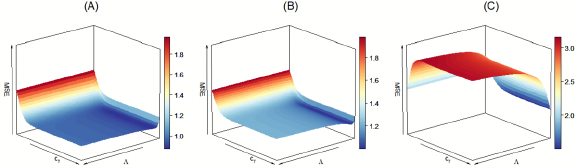
Test-and-pool estimator 1539

Fig B.1. The plots for the mean squared errors in a synthetic example. Leftmost (A) plots

the mean square error mse(Λ,c

; η) of n

1/2

(μ

tap

− μ

) as function of Λ and c

when the null

hypothesis H

holds true (η =0); Middle (B) plots mse(Λ,c

; η) when the null hypothesis H

is weakly violated (η =0.5); Rightmost (C) plots mse(Λ,c

; η) when the null hypothesis H

is strongly violated (η =1.5).

error compared to other choices of Λ. These ﬁndings imply that despite the

bias due to accepting the non-probability sample, the impact would be less

compared to the increased variance due to rejecting the non-probability

sample. But care is needed to determine the amount of information bor-

rowed from the non-probability sample since a small deviation from the

optimal value Λ

∗

can lead to a non-ignorable increase of the mean squared

error. Once the optimal mean squared error is reached at (Λ

∗

), the fur-

ther increment of c

will not be inﬂuential.

c) In the rightmost plot, where H

is strongly violated, the mean squared

error behaves diﬀerently as in (A) and (B). It is advisable to choose both Λ

and c

close to zero (the low probability of combining the non-probability

sample with the probability sample) to minimize the mean squared error.

As above, keeping increasing c

after the mean squared error ﬂattens out

is of no importance.

B.3. Additional simulation results

Table B.1 provides the Monte Carlo averages and standard errors of the data-

adaptive tuned parameters (Λ,c

) and the Monte Carlo proportion of combining

the probability and non-probability samples. Figure B.2 presents the plots of

Monte Carlo biases, variances and mean squared errors of the μ

, μ

eﬀ

, μ

tap

and μ

tap:ﬁx

based on 2000 replicated datasets. For the ﬁxed threshold strategy

μ

tap:ﬁx

, the threshold c

is held ﬁxed to be the 95th quantile of a χ

distribution

(i.e., 3.84) and the tuning parameter Λ is selected by minimizing the asymptotic

mean square error at the ﬁxed c

In Table B.1, we ﬁnd that the adaptive procedure tends to select smaller

values of Λ and c

as b increases. As a result, the Monte Carlo proportions of

combining the probability and non-probability samples together are decreasing,

which is desired for down-weighting the biased non-probability sample. More-

over, we compare the adaptive tuning strategy of c

with a ﬁxed thresholding

strategy, and Figure B.2 shows that the strategy with pre-deﬁned cutoﬀ cannot

1540 C. Gao and S. Yang

Table B.1

Simulation results of Monte Carlo averages of the tuning parameters (Λ,c

) and the

proportion P(comb) of combining the probability and non-probability samples.

Λ c

P(comb)

est se est se est se

holds μ

tap

3.02 4.26 35.06 9.45 0.95 0.22

μ

tap:B

3.05 4.62 35.06 9.44 0.95 0.22

μ

tap:KH

3.06 4.66 35.06 9.44 0.95 0.22

slightly violated μ

tap

2.21 3.39 31.60 13.76 0.86 0.35

μ

tap:B

2.22 3.47 31.60 13.75 0.86 0.35

μ

tap:KH

2.23 3.60 31.60 13.75 0.86 0.35

strongly violated μ

tap

0.16 0.28 1.40 1.97 0.00 0.06

μ

tap:B

0.16 0.28 1.40 1.97 0.00 0.06

μ

tap:KH

0.16 0.28 1.40 1.98 0.00 0.06

Fig B.2. Summary statistics plots of estimators of μ

with respect to the strength of violation,

labeled by b. Each column of the plots corresponds to a diﬀerent metric: “bias” for bias, “var”

for variance, “MSE” for mean square error.

satisfactorily control the mean squared error when H

is slightly or strongly

violated.

B.4. Double-bootstrap procedure for v

selection

Following the algorithm mentioned by [10], where optimal v

is selected to en-

sure the coverage probability, we need to retain the K bootstrapped samples,

called V

(1)

(2)

, ···,V

(K)

where V

(b)

= {V

=(X

(b)

(b)

)



: i ∈ 1, ···,n},b=

1, ···,K with n = n

. The reason it is called double bootstrap is that each

bootstrap sample spawns itself to a set of K



second-order bootstrap samples.

Next, we set up the candidates for v

. Under the assumption (A2), we let v

be the form of κ log log n with κ ∈{2, 4, 10, 20, 30}, and construct the bound-

based adaptive conﬁdence intervals for each given κ at 1 − α conﬁdence level,

denoted as C

PACI,κ

,1−α

(a). Given each κ, we compute the coverage probability for

the associated adaptive conﬁdence intervals regarding these K



second-ordered

simulated datasets. Then, choose the smallest κ that ensures the actual cov-

Test-and-pool estimator 1541

erage probability larger than 1 − α. Speciﬁcally, we use the estimator μ

(b)

for

in each bootstrapped dataset as the ground truth and count the number of

datasets in which the adaptive conﬁdence interval covers the ground truth, say

c(κ)=





b=1

1{μ

(b)

∈ C

PACI,κ,(b)

,1−α

(a)} and therefore the v

can be determined

by using v

=inf{κ : c(κ)/K



> 1 − α}×log log n. In our simulation, K



is set

to be 100.

B.5. Details of the Bayesian method

In this section, we provide the details of the Bayesian approaches proposed by

[52] to combine the probability and non-probability samples as follows.

1. Solve the score function for β by using the non-probability sample:



NPR

=argmin



i=1

B,i

− X



β)=0.

2. Construct the informative prior with three choices:

Prior 1: Choose a weakly informative parameterization of the prior as

β ∼N(0, 10

which can be treated as a reference for comparison.

Prior 2: Let



be the solution to the score function based on the probability

sample



=argmin



i=1

A,i

− X



β)=0.

Then consider the squared Euclidean distance between



and



NPR

as the hyper-parameter σ

for the variance of β:

β ∼N





NPR

, diag(



−



NPR



)



Prior 3: In lieu of using the squared distance to extract information on σ

a nonparametric with-replacement bootstrap procedure can be im-

plemented (B = 1000). After estimating the coeﬃcient in each of

them, denoted by



(i)

NPR

, one replication-based variance estimator can

be obtained, σ

NPR



i=1

(



(i)

NPR

−



NPR

)

/(B − 1) with



NPR

1/B



i=1



(i)

NPR

. Then, the informative prior can be constructed

β ∼N(



NPR

p×p

· σ

NPR

3. Assume that the model for the observed probability sample is

| δ

A,i

=1∼N(X



β,σ

1542 C. Gao and S. Yang

By imposing an informative non-probability-based prior, the resulting pos-

terior estimates are expected to be more eﬃcient. Speciﬁcally, these priors

are:

β ∼N(β

,σ

),σ

−2

∼ Γ(r, m),r= m =10

−3

where

Prior 1: β

=0,σ

=10

Prior 2: β



NPR

,σ

= diag(



−



NPR



Prior 3: β



NPR

,σ

= I

p×p

· σ

NPR

The posterior Markov chain Monte Carlo (MCMC) samples of β and Y

are ob-

tained by drawing 2000 samples from the posterior distributions and discarding

the ﬁrst 500 samples as the burn-in procedures. The Bayesian estimator is

μ

Bayes

=1/





i=1

with



N =



i=1

where

is the posterior mean calculated by

=1/(2000 − 500)



2000

k=501

i,k

Borrowed from Bayes’ Theorem, its variance and 95% highest posterior density

intervals can be estimated via the MCMC posterior samples. Denote μ

Bayes,k





i=1

i,k

,k = 501, ···, 2000. Then, we have

var(μ

Bayes

2000 − 500 − 1

2000



k=501

(μ

Bayes,k

− μ

Bayes

)

HPDI = {Q(μ

Bayes,k

; α/2),Q(μ

Bayes,k

;1− α/2)},

where Q(μ

Bayes,k

; α

)representstheα

-th sample quantile of the posterior sam-

ples μ

Bayes,k

, k = 501, ···, 2000 after burn-in.

References

[1] Abramowitz, M., Stegun, I. A. and Romer, R. H. (1988). Handbook

of mathematical functions with formulas, graphs, and mathematical tables.

[2] Baker, R., Brick, J. M., Bates, N. A., Battaglia, M.,

Couper, M. P., Dever, J. A., Gile, K. J. and Tourangeau, R. (2013).

Summary report of the AAPOR task force on non-probability sampling.

Journal of Survey Statistics and Methodology 1 90–143.

[3] Baltagi, B. H., Bresson, G. and Pirotte, A. (2003). Fixed eﬀects, ran-

dom eﬀects or Hausman–Taylor?: A pretest estimator. Economics Letters

79 361–369.

[4] Barr, D. R. and Sherrill, E. T. (1999). Mean and variance of truncated

normal distributions. The American Statistician 53 357–361.

Test-and-pool estimator 1543

[5] Beaumont, J.-F. (2020). Are probability surveys bound to disappear for

the production of oﬃcial statistics? Survey Methodology 46 1–28.

[6] Bethlehem, J. (2016). Solving the nonresponse problem with sample

matching? Social Science Computer Review 34 59–77.

[7] Binder, D. A. and Roberts, G. R. (2003). Design-based and model-

based methods for estimating model parameters. Analysis of Survey Data

29 33–54. MR1978842

[8] Boas, M. L. (2006). Mathematical Methods in the Physical Sciences.John

Wiley & Sons.

[9] Boos, D. D. and Stefanski, L. A. (2013). Essential Statistical Inference:

Theory and Methods 591. Springer. MR3024617

[10] Chakraborty, B., Laber, E. B. and Zhao, Y. (2013). Inference for

optimal dynamic treatment regimes using an adaptive m-out-of-n bootstrap

scheme. Biometrics 69 714–723. MR3106599

[11] Chen, S., Yang, S. and Kim, J. K. (2022). Nonparametric mass imputa-

tion for data integration. Journal of survey statistics and methodology 10

1–24.

[12] Chen, Y., Li, P. and Wu, C. (2019). Doubly Robust Inference With Non-

probability Survey Samples. Journal of the American Statistical Association

115 2011–2021. MR4189773

[13] Cheng, X. (2008). Robust conﬁdence intervals in nonlinear regression un-

der weak identiﬁcation. Manuscript, Department of Economics, Yale Uni-

versity.

[14] Citro, C. F. (2014). From multiple modes for surveys to multiple data

sources for estimates. Survey Methodology 40 137–161.

[15] Cochran, W. G. (2007). Sampling Techniques, 3 ed. New York: John

Wiley & Sons, Inc. MR0054199

[16] Colnet, B., Mayer, I.,

Chen, G., Dieng, A., Li, R., Varoquaux, G.,

Vert, J.-P., Josse, J. and Yang, S. (2020). Causal inference methods

for combining randomized trials and observational studies: a review. arXiv

preprint arXiv:2011.08047.

[17] Couper, M. P. (2000). Web surveys: A review of issues and approaches.

The Public Opinion Quarterly 64 464–494.

[18] Couper, M. P. (2013). Is the sky falling? New technology, changing media,

and the future of surveys. Survey Research Methods 7 145–156.

[19] Deville, J.-C. and Särndal, C.-E. (1992). Calibration estimators in sur-

vey sampling. Journal of the American Statistical Association 87 376–382.

MR1173804

[20] Elliot,M.R.(2009). Combining data from probability and non-

probability samples using pseudo-weights. Survey Practice 2 2982.

[21] Elliott, M. N. and Haviland, A. (2007). Use of a web-based conve-

nience sample to supplement a probability sample. Survey Methodology 33

211–215.

[22] Elliott, M. R. (2007). Bayesian weight trimming for generalized linear

regression models. Survey Methodology 33 23–34.

[23] Elliott, M. R., Valliant, R. et al. (2017). Inference for nonprobability

1544 C. Gao and S. Yang

samples. Statistical Science 32 249–264. MR3648958

[24] Fuller, W. A. (2009). Sampling Statistics. Wiley, Hoboken, NJ.

[25] Gao, C., Yang, S. and Kim, J. K. (2023). Soft calibration

for selection bias problems under mixed-eﬀects models. Biometrika

doi.org/10.1093/biomet/asad016.

[26] Haziza, D. and Rao, J. N. (2006). A nonresponse model approach to

inference under imputation for missing survey data. Survey Methodology

32 53–64. MR2193025

[27] Kalton, G. (1983). Models in the practice of survey sampling. Interna-

tional Statistical Review/Revue Internationale de Statistique 51 175–188.

[28] Kalton, G. (2019). Developments in survey research over the past 60

years: A personal perspective. International Statistical Review 87 S10–S30.

MR3957341

[29] Kim, J. K. and Haziza, D. (2014). Doubly robust inference with missing

data in survey sampling. Statistica Sinica 24 375–394. MR3183689

[30] Kim, J. K. and Wang, Z. (2019). Sampling techniques for big data anal-

ysis. International Statistical Review 87 S177–S191. MR3957350

[31] Kott, P. S. (2006). Using calibration weighting to adjust for nonresponse

and coverage errors. Survey Methodology 32 133–142.

[32] Laber, E. B., Lizotte,D.J., Qian, M., Pelham,W.E.and Mur-

phy, S. A. (2014). Dynamic treatment regimes: Technical challenges and

applications. Electronic Journal of Statistics 8 1225–1272. MR3263118

[33] Laber, E. B. and Murphy, S. A. (2011). Adaptive conﬁdence intervals

for the test error in classiﬁcation. Journal of the American Statistical As-

sociation 106 904–913. MR2894746

[34] Little, R. J. (1982). Models for nonresponse in sample surveys. Journal

of the American statistical Association 77 237–250. MR0664675

[35] Mashreghi, Z., Léger, C. and Haziza, D. (2014). Bootstrap methods

for imputed data from regression, ratio and hot-deck imputation. Canadian

Journal of Statistics 42 142–167. MR3181587

[36] McRoberts, R. E., Tomppo,E.O.and Næsset, E. (2010). Advances

and emerging issues in national forest inventories. Scandinavian Journal of

Forest Research 25 368–381.

[37] Molina, E., Smith, T. and Sugden, R. (2001). Modelling overdispersion

for complex survey data. International Statistical Review 69 373–384.

[38] Mosteller, F. (1948). On pooling data. Journal of the American Statis-

tical Association 43 231–242.

[39] Nelder,J.A.and Mead, R. (1965). A simplex method for function

minimization. The Computer Journal 7 308–313. MR3363409

[40] Palmer, J. R., Espenshade, T. J., Bartumeus, F., Chung, C. Y.,

Ozgencil,N.E.and Li, K. (2013). New approaches to human mobility:

Using mobile phones for demographic research. Demography 50 1105–1128.

[41] Pfeffermann, D., Eltinge, J. L., Brown, L. D. and Pfeffer-

mann, D. (2015). Methodological issues and challenges in the production

of oﬃcial statistics: 24th Annual Morris Hansen Lecture. Journal of Survey

Statistics and Methodology 3 425–483.

Test-and-pool estimator 1545

[42] Rao, J. (2020). On making valid inferences by integrating data from sur-

veys and other sources. Sankhya B 83 242–272. MR4256318

[43] Rao, J., Wu, C. and Yue, K. (1992). Some recent work on resampling

methods for complex surveys. Survey Methodology 18 209–217.

[44] Rao, J. N. (2014). Small-area estimation. Wiley StatsRef: Statistics Ref-

erence Online. MR1953089

[45] Rao, R. R. (1962). Relations between weak and uniform convergence

of measures with applications. The Annals of Mathematical Statistics 33

659–680. MR0137809

[46] Rivers, D. (2007). Sample Matching for Web Surveys: Theory and Appli-

cation. In Joint Statistical Meetings.

[47] Robbins, M. W., Ghosh-Dastidar, B. and Ramchand, R. (2021).

Blending of Probability and Non-Probability Samples: Applications to a

Survey of Military Caregivers. Journal of Survey Statistics and Methodol-

ogy 9 1114–1145. MR4417203

[48] Robins, J. M. (2004). Optimal structural nested models for optimal se-

quential decisions. In Proceedings of the Second Seattle Symposium in Bio-

statistics 179 189–326. Springer. MR2129402

[49] Robins,J.M., Rotnitzky, A. and Zhao,L.P.(1994). Estimation

of regression coeﬃcients when some regressors are not always observed.

Journal of the American Statistical Association 89 846–866. MR1294730

[50] Rosenbaum, P. R. and Rubin, D. B. (1983). The central role of the

propensity score in observational studies for causal eﬀects. Biometrika 70

41–55. MR0742974

[51] Rothwell, P. M. (2005). Subgroup analysis in randomised controlled tri-

als: importance, indications, and interpretation. The Lancet 365 176–186.

[52] Sakshaug, J. W., Wiśniowski, A., Ruiz,D.A.P.and Blom,A.G.

(2019). Supplementing Small Probability Samples with Nonprobability

Samples: A Bayesian Approach. Journal of Oﬃcial Statistics 35 653–681.

[53] Särndal, C.-E., Swensson, B. and Wretman, J. (2003). Model Assisted

Survey Sampling. New York: Springer-Verlag. MR1140409

[54] Scharfstein, D. O., Rotnitzky, A. and Robins,J.M.(1999). Adjust-

ing for nonignorable drop-out using semiparametric nonresponse models.

Journal of the American Statistical Association 94 1096–1120. MR1731478

[55] Schenker, N. and Welsh, A. (1988). Asymptotic results for multiple

imputation. Annals of Statistics 16 1550–1566. MR0964938

[56] Shao, J. (1994). Bootstrap sample size in nonregular cases. Proceedings of

the American Mathematical Society 122 1251–1262. MR1227529

[57] Shao, J. and Tu, D. (2012). The Jackknife and Bootstrap. Springer, New

York. MR1351010

[58] Skinner, C. et al. (1992). Pseudo-likelihood and quasi-likelihood estima-

tion for complex sampling schemes. Computational Statistics & Data Anal-

ysis 13 395–405. MR1173330

[59] Staiger, D. and Stock, J. H. (1997). Instrumental variables regression

with weak instruments. Econometrica 65 557–586. MR1445622

[60] Tallis, G. (1963). Elliptical and radial truncation in normal populations.

1546 C. Gao and S. Yang

The Annals of Mathematical Statistics 34 940–944. MR0152081

[61] Tam, S.-M. and Clarke, F. (2015). Big data, oﬃcial statistics and some

initiatives by the Australian Bureau of Statistics. International Statistical

Review 83 436–448.

[62] Tourangeau, R., Conrad, F. G. and Couper,M.P.(2013). The

Science of Web Surveys. Oxford University Press: New York.

[63] Toyoda, T. and Wallace, T. D. (1979). Pre-testing on part of the data.

Journal of Econometrics 10 119–123. MR0567944

[64] Tsiatis, A. (2006). Semiparametric Theory and Missing Data. Springer,

New York. MR2233926

[65] van der Vaart (2000). Asymptotic Statistics 3. Cambridge university

press, Cambridge: Cambridge University Press. MR1652247

[66] Vavr ec k, L. and Rivers, D. (2008). The 2006 cooperative congres-

sional election study. Journal of Elections, Public Opinion and Parties 18

355–366.

[67] Vermeulen, K. and Vansteelandt, S. (2015). Bias-reduced doubly

robust estimation. Journal of the American Statistical Association 110

1024–1036. MR3420681

[68] Wallace, T. D. (1977). Pretest estimation in regression: A survey. Amer-

ican Journal of Agricultural Economics 59 431–443.

[69] Williams, D. and Brick, J. M. (2018). Trends in US face-to-face house-

hold survey nonresponse and level of eﬀort. Journal of Survey Statistics

and Methodology 6 186–211.

[70] Xu, C., Chen, J. and Harold, M. (2013). Pseudo-likelihood-based

Bayesian information criterion for variable selection in survey data. Survey

Methodology 39 303–322.

[71] Yang, S. and Ding, P. (2020). Combining multiple observational data

sources to estimate causal eﬀects. Journal of the American Statistical As-

sociation 115 1540–1554. MR4143484

[72] Yang, S., Gao, C., Zeng, D. and Wang, X. (2022). Elastic integrative

analysis of randomized trial and real-world data for treatment heterogeneity

estimation. Journal of the Royal Statistical Society: Series B (Statistical

Methodology), In press.

[73] Yang, S. and Kim, J. K. (2020). Statistical data integration in survey

sampling: A review. Japanese Journal of Statistics and Data Science 3

625–650. MR4181993

[74] Yang, S., Kim, J. K. and Hwang, Y. (2021). Integration of survey data

and big observational data for ﬁnite population inference using mass im-

putation. Survey Methodology 47 29–58.

[75] Yang, S., Kim, J. K. and Song, R. (2020). Doubly robust inference when

combining probability and non-probability samples with high dimensional

data. Journal of the Royal Statistical Society: Series B (Statistical Method-

ology) 82 445–465. MR4084171