
This article was downloaded by: [Northwestern University]
On: 16 June 2014, At: 12:41
Publisher: Routledge
Informa Ltd Registered in England and Wales Registered Number: 1072954
Registered office: Mortimer House, 37-41 Mortimer Street, London W1T 3JH,
UK
Journal of Research on
Educational Effectiveness
Publication details, including instructions for
authors and subscription information:
http://www.tandfonline.com/loi/uree20
Performance Trajectories
and Performance Gaps as
Achievement Effect-Size
Benchmarks for Educational
Interventions
Howard S. Bloom
a
, Carolyn J. Hill
b
, Alison Rebeck
Black
a
& Mark W. Lipsey
c
a
MDRC , New York, New York, USA
b
Georgetown Public Policy Institute , Washington,
DC, USA
c
Center for Evaluation Research and Methodology ,
Vanderbilt Institute for Public Policy Studies ,
Nashville, Tennessee, USA
Published online: 13 Oct 2008.
To cite this article: Howard S. Bloom , Carolyn J. Hill , Alison Rebeck Black & Mark W.
Lipsey (2008) Performance Trajectories and Performance Gaps as Achievement Effect-
Size Benchmarks for Educational Interventions, Journal of Research on Educational
Effectiveness, 1:4, 289-328, DOI: 10.1080/19345740802400072
To link to this article: http://dx.doi.org/10.1080/19345740802400072
PLEASE SCROLL DOWN FOR ARTICLE
Taylor & Francis makes every effort to ensure the accuracy of all the
information (the “Content”) contained in the publications on our platform.
However, Taylor & Francis, our agents, and our licensors make no
representations or warranties whatsoever as to the accuracy, completeness,

or suitability for any purpose of the Content. Any opinions and views
expressed in this publication are the opinions and views of the authors, and
are not the views of or endorsed by Taylor & Francis. The accuracy of the
Content should not be relied upon and should be independently verified with
primary sources of information. Taylor and Francis shall not be liable for any
losses, actions, claims, proceedings, demands, costs, expenses, damages,
and other liabilities whatsoever or howsoever caused arising directly or
indirectly in connection with, in relation to or arising out of the use of the
Content.
This article may be used for research, teaching, and private study purposes.
Any substantial or systematic reproduction, redistribution, reselling, loan,
sub-licensing, systematic supply, or distribution in any form to anyone is
expressly forbidden. Terms & Conditions of access and use can be found at
http://www.tandfonline.com/page/terms-and-conditions
Downloaded by [Northwestern University] at 12:41 16 June 2014

Journal of Research on Educational Effectiveness, 1: 289–328, 2008
Copyright © Taylor & Francis Group, LLC
ISSN: 1934-5747 print / 1934-5739 online
DOI: 10.1080/19345740802400072
Performance Trajectories and Performance Gaps as
Achievement Effect-Size Benchmarks for
Educational Interventions
Howard S. Bloom
MDRC, New York, New York, USA
Carolyn J. Hill
Georgetown Public Policy Institute, Washington, DC, USA
Alison Rebeck Black
MDRC, New York, New York, USA
Mark W. Lipsey
Center for Evaluation Research and Methodology, Vanderbilt Institute for Public
Policy Studies, Nashville, Tennessee, USA
Abstract: Two complementary approaches to developing empirical benchmarks for
achievement effect sizes in educational interventions are explored. The first approach
characterizes the natural developmental progress in achievement made by students from
one year to the next as effect sizes. Data for seven nationally standardized achievement
tests show large annual gains in the early elementary grades followed by gradually
declining gains in later grades. A given intervention effect will therefore look quite
different when compared to the annual progress for different grade levels. The sec-
ond approach explores achievement gaps for policy-relevant subgroups of students or
schools. Data from national- and district-level achievement tests show that, when rep-
resented as effect sizes, student gaps are relatively small for gender and much larger for
economic disadvantage and race/ethnicity. For schools, the differences between weak
schools and average schools are surprisingly modest when expressed as student-level
effect sizes. A given intervention effect viewed in terms of its potential for closing one
of these performance gaps will therefore look very different depending on which gap is
considered.
Keywords: Effect size, student performance, educational evaluation
Address correspondence to Howard S. Bloom, MDRC, 16 East 34th Street, 19th
Floor, New York, NY 10016, USA. E-mail: how[email protected]
Downloaded by [Northwestern University] at 12:41 16 June 2014
290 H. S. Bloom et al.
In educational research, the effect of an intervention on academic achievement
is often expressed as an effect size. The most common effect size metric for this
purpose is the standardized mean difference,
1
which is defined as the difference
between the mean outcome for the intervention group and that for the control
or comparison group divided by the common within group standard deviation
of that outcome. This effect size metric is a statistic and, as such, represents
the magnitude of an intervention in statistical terms, specifically in terms of
the number of standard deviation units by which the intervention group outper-
forms the control group. That statistical magnitude, however, has no inherent
meaning for the practical or substantive magnitude of the intervention effect
in the context of its application. How many standard deviations of difference
represent an improvement in achievement that matters to the students, parents,
teachers, administrators, or policymakers who may question the value of that
intervention?
Assessing the practical or substantive magnitude of an effect size is central
to three stages of educational research. It arises first when the research is being
designed and decisions must be made about how much statistical precision or
power is needed. Such decisions are framed in terms of the minimum effect
size that the study should be able to detect with a given level of confidence.
The smaller the desired “minimum detectable effect,” the larger the study
sample must be. But how should one choose and justify a minimum effect size
estimate for this purpose? The answer to this question usually revolves around
consideration of what effect size would represent a practical effect of sufficient
importance in the intervention context that it would be negligent if the research
failed to identify it at a statistically significant level.
The issue of interpretation arises next toward the end of a study when re-
searchers are trying to decide whether the intervention effects they are reporting
are large enough to be substantively important or policy relevant. Here also the
simple statistical representation of the number of standard deviation units of
improvement produced by the intervention begs the question of what it means
in practical terms. This issue of interpretation arises yet again when researchers
attempt to synthesize estimates of intervention effects from a series of studies
in a meta-analysis. The mean effect size across studies of an intervention that
summarizes the overall findings is also only a statistical representation that
must be interpreted in practical or substantive terms for its importance to be
properly understood.
To interpret the practical or substantive magnitude of effect sizes, it is nec-
essary to invoke some appropriate frame of reference external to their statistical
1
For discussions of alternative effect size metrics, see Cohen (1988); Fleiss (1994);
Glass, McGaw, and Smith (1981); Grissom and Kim (2005); Hedges and Olkin (1985);
Lipsey and Wilson (2001); Rosenthal (1991, 1994); and Rosenthal, Rosnow, and Rubin
(2000).
Downloaded by [Northwestern University] at 12:41 16 June 2014
Achievement Effect-Size Benchmarks 291
representation that can, nonetheless, be connected to that statistical representa-
tion. There is no inherent practical or substantive meaning to standard deviation
units. To interpret them we must have benchmarks that mark off magnitudes of
recognized practical or substantive significance in standard deviation units. We
can then assess an intervention effect size with those benchmarks. There are
many substantive frames of reference that can provide benchmarks that might
be used for this purpose, however, and no one will be best for every intervention
circumstance.
This article develops and explores two types of empirical benchmarks
that have broad applicability for interpreting intervention effect sizes for stan-
dardized achievement tests in educational research. One benchmark considers
those effect sizes relative to the normal achievement gains children make from
one year to the next. The other considers them in relation to policy relevant
achievement gaps between subgroups of students and schools achieving be-
low normative levels and those whose achievement represents those normative
levels. Before discussing these benchmarks, however, we must first consider
several related issues that provide important contextual background for that
discussion.
EFFECT SIZE VARIANTS, STATISTICAL SIGNIFICANCE,
AND INAPPROPRIATE RULES OF THUMB
Standardized and Unstandardized Effect Estimates
Standardized effect size statistics are not the only way to report the empirical
effects of an educational intervention. Such effects can also be reported in the
original metric in which the outcomes were measured. There are two main
situations in which standardized effect sizes can improve the interpretability of
impact estimates. The first is when outcome measures do not have inherently
meaningful metrics. For example, many social and emotional outcome scales
for preschoolers do not relate to recognized developmental characteristics in a
way that would make their numerical values inherently meaningful. Most stan-
dardized achievement measures are similar in this regard. Only someone with
a great deal of experience using them to assess students whose academic per-
formance was familiar would find the numerical scores directly interpretable.
Such scores generally take on meaning only when used to rank students or
compare student groups. Standardizing effect estimates on such measures rel-
ative to their variation can make them at least somewhat more interpretable. In
contrast, outcome measures for vocational education programs—like earnings
(in dollars) or employment rates (percentages)—have numeric values that rep-
resent units that are widely known and understood. Standardizing results for
these kinds of measures can make them less interpretable and should not be
done without a compelling reason.
Downloaded by [Northwestern University] at 12:41 16 June 2014
292 H. S. Bloom et al.
A second situation in which it can be helpful to standardize effects is
when it is important to compare or combine effects observed on different
measures of the same construct. This often occurs in research syntheses when
different studies measure a common outcome in different ways, for example,
with different standardized achievement tests. The situation also can arise in
single studies that use multiple measures of a given outcome. In these cases,
standardizing the effect sizes can facilitate comparison and interpretation.
Standardizing on Different Standard Deviations
What makes standardized mean difference effect sizes comparable across dif-
ferent outcome measures is that they are all standardized using standard de-
viations for the same unit and assume that those standard deviations estimate
the variation for the same population of such units. In educational research,
the units are typically students, assumed drawn from some relevant population
of students, and the standard deviation for the distribution of student scores is
used as the denominator of the effect size statistic. Other units over which the
outcome scores vary can be used for the standardization, however, and there
may be more than one reference population that might be represented by those
scores. There is no clear consensus in the literature about which standard de-
viation to use for standardizing effect sizes for educational interventions, but
when different ones are used it is difficult to properly compare them across
studies. The following examples illustrate the nature of this problem.
Researchers can compute effect sizes using standard deviations for a study
sample or for a larger population. This choice arises, for example, when na-
tionally normed tests are used to measure student achievement and the norming
data provide estimates of the standard deviation for the national population.
Theoretically, a national standard deviation might be preferable for standard-
izing impact estimates because it provides a consistent and universal point of
reference. That assumes, of course, that the appropriate reference population for
a particular intervention study is the national population. A national standard
deviation will generally be larger than that for study samples, however, and
thereby will tend to make effect sizes “look smaller” than if they were based on
the study sample. If everyone used the same standard deviation this would not
be a problem, but this has not been the case to date. Even if researchers agreed
to use national standard deviations for measures from nationally normed tests,
they would still have to use sample-based standard deviations for other mea-
sures. Consequently, it would remain difficult to compare effect sizes across
those different measures.
Another type of choice concerning the standard deviation is whether to
use student-level standard deviations or classroom-level or school-level stan-
dard deviations to compute effect sizes. Because student-level standard devi-
ations are typically several times the size of their school-level counterparts,
Downloaded by [Northwestern University] at 12:41 16 June 2014

Achievement Effect-Size Benchmarks 293
this difference markedly affects the magnitudes of effect sizes.
2
Most studies
use student-level standard deviations. But studies that are based on aggregate
school-level data and do not have access to student-level information can only
use school-level standard deviations. Also, when the locus of the intervention
is the classroom or the whole school, researchers often choose to analyze the
results at that level and use the corresponding standard deviations for the effect
size estimates (although this is not necessary). Comparisons of effect sizes that
standardize on standard deviations for different units can be very misleading
and can only be done if one or the other is converted so that they represent the
same unit.
Yet another choice concerns whether to use standard deviations for ob-
served outcome measures to compute effect sizes or reliability-adjusted stan-
dard deviations for underlying “true scores.” Theoretically, it is preferable to
use standard deviations for true scores because they represent the actual diver-
sity of subjects with respect to the construct being measured without distortion
by measurement error, which can vary from measure to measure and from
study to study. Practically, however, there are often no comprehensive esti-
mates of reliability to make appropriate adjustments for all relevant sources of
measurement error.
3
To place this issue in context, note that if the reliability
of a measure is 0.75 then the standard deviation of its true score is
√
0.75—or
roughly 0.87—times the standard deviation of its observed score.
Other ways that standard deviations used to compute effect sizes can dif-
fer include regression-adjusted versus unadjusted standard deviations, pooled
standard deviations for students within given school districts or states versus
those which include interdistrict and/or interstate variation, and standard devi-
ations for the control group of a study versus that for the pooled variation in its
treatment group and control group.
We highlight the preceding inconsistencies among the choices of standard
deviations for effect size computations not because we think they can be re-
solved readily but rather because we believe they should be recognized more
2
The standard deviation for individual students can be more than twice that for school
means. This is the case, for example, if the intraclass correlation of scores for students
within schools is about 0.20 and there are about 80 students in a grade per school.
Intraclass correlations and class sizes in this range are typical (e.g., Bloom, Richburg-
Hayes, & Black, 2007; Hedges & Hedberg, 2007).
3
A comprehensive assessment of measurement reliability based on generalizabil-
ity theory (Brennan, 2001; Shavelson & Webb, 1991 or Cronbach, Gleser, Nanda, &
Rajaratnam, 1972) would account for all sources of random error, including, where
appropriate, rater inconsistency, temporal instability, item differences, and all relevant
interactions. Typical assessments of measurement reliability in the literature are based on
classical measurement theory (e.g., Nunnally, 1967), which only deals with one source
of measurement error at a time. Comprehensive assessments thereby yield substantially
lower values for coefficients of reliability.
Downloaded by [Northwestern University] at 12:41 16 June 2014
294 H. S. Bloom et al.
widely. Often, researchers do not specify which standard deviations are used
to calculate effect sizes, making it impossible to know whether they can be
appropriately compared across studies. Thus, we urge researchers to clearly
specify the standard deviations they use to compute effect sizes.
Statistical Significance
A third contextual issue has to do with the appropriate role of statistical sig-
nificance in the interpretation of estimates of intervention effects. This issue
highlights the confusion that has existed for decades about the limitations of
statistical significance testing for gauging intervention effects. This confusion
reflects, in part, differences between the framework for statistical inference de-
veloped by Fisher (1949), which focuses on testing a specific null hypothesis of
zero effect against a general alternative hypothesis of nonzero effect, versus the
framework developed by Neyman and Pearson (1928, 1933), which focuses on
both a specific null hypothesis and a specific alternative hypothesis (or effect
size).
The statistical significance of an estimated intervention effect is the prob-
ability that an estimate as large as or larger than that observed would occur
by chance if the true effect were zero. When this probability is less than 0.05,
researchers conventionally conclude that the null hypothesis of “no effect” has
been disproven. However determining that an effect is not likely to be zero
does not provide any information about its magnitude—how much larger than
zero it is. Rather it is the effect size (standardized or not) that provides this
information. Therefore, to properly interpret an estimated intervention effect
one should first determine whether it is statistically significant—indicating that
a nonzero effect likely exists—and then assess its magnitude. An effect size
statistic can be used to describe its statistical magnitude but, as we have in-
dicated, assessing its practical or substantive magnitude will require that it be
compared with some benchmark derived from relevant practical or substantive
considerations.
Rules of Thumb
This brings us to the core question for this article: What benchmarks are relevant
and useful for purposes of interpreting the practical or substantive magnitude
of the effects of educational interventions on student achievement? The most
common practice is to rely on Cohen’s suggestion that effect sizes of about
0.20, 0.50, and 0.80 standard deviations be considered small, medium, and
large, respectively. These guidelines do not derive from any obvious context
of relevance to intervention effects in education, and Cohen (1988) himself
clearly stated that his suggestions were “for use only when no better basis for
Downloaded by [Northwestern University] at 12:41 16 June 2014
Achievement Effect-Size Benchmarks 295
estimating the ES index is available” (p. 25). Nonetheless, these guidelines of
last resort have provided the rationale for countless interpretations of findings
and sample size decisions in education research.
Cohen based his guidelines on his general impression of the distribution
of effect sizes for the broad range of social science studies that compared two
groups on some measure. For instances where the groups represent treatment
and control conditions in intervention studies, Lipsey (1990) provided empir-
ical support for Cohen’s estimates using results from 186 meta-analyses of
6,700 studies of educational, psychological, and behavioral interventions. The
bottom third of the distribution of effect sizes from these meta-analyses ranged
from 0.00 to 0.32 standard deviation, the middle third ranged from 0.33 to
0.55 standard deviation, and the top third ranged from 0.56 to 1.20 standard
deviation.
Both Cohen’s suggested default values and Lipsey’s empirical estimates
were intended to describe a wide range of research in the social and behavioral
sciences. There is no reason to believe that they necessarily apply to the effects
of educational interventions or, more specifically, to effects on the standard-
ized achievement tests widely used as outcome measures for studies of such
interventions.
For education research, a widely cited benchmark is that an effect size of
0.25 is required for an intervention effect to have “educational significance.” We
have attempted to trace the source of this claim and can find no clear reference
to it prior to a document authored by Tallmadge (1977) that provided advice
for preparing applications for funding by what was then the U.S. Department
of Health, Education, and Welfare. That document included the following
statement: “One widely applied rule is that the effect must equal or exceed
some proportion of a standard deviation—usually one-third, but at times as
small as one-fourth—to be considered educationally significant” (p. 34). No
other justification or empirical support was provided for this statement.
Reliance on rules of thumb such as those provided by Cohen or cited
in Tallmadge for assessing the magnitude of the effects of educational inter-
ventions is not justified by any support that these authors provide for their
relevance to that context or any demonstration of such relevance that has been
presented subsequently. With such considerations in mind, we have undertaken
a project to develop more comprehensive empirical benchmarks for gauging
effect sizes for the achievement outcomes of educational interventions. These
benchmarks are being developed from three complementary perspectives: (a)
relative to the magnitudes of normal annual student academic growth, (b) rela-
tive to the magnitudes of policy-relevant gaps in student performance, and (c)
relative to the magnitudes of the achievement effect sizes that have been found
in past educational interventions. Benchmarks from the first perspective will
help to answer questions like, How large is the effect of a given intervention
if we think about it in terms of what it might add to a year of “normal” stu-
dent academic growth? Benchmarks from the second perspective will help to
Downloaded by [Northwestern University] at 12:41 16 June 2014
296 H. S. Bloom et al.
answer questions like, How large is the effect if we think about it in terms of
narrowing a policy-relevant gap in student performance? Benchmarks from the
third perspective will help to answer questions like, How large is the effect of a
given intervention if we think about it in terms of what prior interventions have
been able to accomplish? A fourth perspective, which we are not exploring
because good work on it is being done by others (e.g., Duncan & Magnuson,
2007; Harris, 2008; Ludwig & Phillips, 2007), is that of cost–benefit analysis
or cost-effectiveness analysis. Benchmarks from this perspective will help to
answer questions like, Do the benefits of a given intervention—for example, in
terms of increased lifetime earnings—outweigh its costs? Or is Intervention A
a more cost-effective way to produce a given academic gain than Intervention
B?
The following sections present benchmarks developed from the first two
perspectives just described, based on analyses of trajectories of student per-
formance across the school years and performance gaps between policy rel-
evant subgroups of students and schools. Our companion article will present
benchmarks from the third perspective, based on studies of the effects of past
educational interventions (Lipsey, Bloom, Hill and Black, in preparation).
BENCHMARKING AGAINST NORMATIVE EXPECTATIONS FOR
ACADEMIC GROWTH
Our first benchmark compares the effects of educational interventions to the
natural growth in academic achievement that occurs during a year of life for an
average student in the United States, building on the approach of Kane (2004).
This analysis measures the growth in average student achievement from one
spring to the next. The growth that occurs during this period reflects the effects
of attending school plus the many other developmental influences that students
experience during any given year.
Effect sizes for year-to-year growth were determined from national norm-
ing studies for seven standardized tests of reading plus corresponding informa-
tion for math, science, and social studies from six of these tests.
4
The required
information was obtained from technical manuals for each test. Because it is
the scaled scores that are comparable across grades, the effect sizes were com-
puted from the mean scaled scores and the pooled standard deviations for each
4
The seven tests analyzed for reading were the CAT5 (1991 norming sample), the
Stanford Achievement Test, SAT9 (1995 norming sample), the Terra Nova-CTBS (1996
norming sample), the Gates–MacGinitie (1998–1999 norming sample), the Metropolitan
Achievement Test, MAT8 (1999–2000 norming sample), the Terra Nova-CAT (1999–
2000 norming sample), and the SAT10 (2002 norming sample). The math, science, and
social studies tests included all these except the Gates–MacGinitie.
Downloaded by [Northwestern University] at 12:41 16 June 2014

Achievement Effect-Size Benchmarks 297
pair of adjacent grades.
5
The reading component of the California Achieve-
ment Test, 5th Edition (CAT5), for example, has a spring national mean scaled
score for kindergarten of 550 with a standard deviation of 47.4 and a first-grade
spring mean scale score of 614 with a standard deviation of 45.4. The dif-
ference in mean scaled scores—or growth—for the spring-to-spring transition
from kindergarten to first grade is therefore 64 points. Dividing this growth by
the pooled standard deviation for the two grades yields an effect size for the
K-1 transition of 1.39 standard deviations. Calculations like these were made
for all K-12 transitions for all tests and academic subject areas with available
information.
Effect size estimates are determined both by their numerators (the differ-
ence between means) and their denominators (the pooled standard deviation).
Hence, the question will arise as to which factor contributes most to the grade-
to-grade transition patterns found for these achievement tests. Because the
standard deviations for each test examined are stable across grades K-12 (see
Appendix Table A1) the effect sizes reported are determined almost entirely
by differences between grades in mean scaled scores.
6
In other words, it is the
variation in growth of measured student achievement across grades K-12 that
produces the reported pattern of grade-to-grade effect sizes, not differences in
standard deviations across grades.
7
Indeed, the declining change in scale scores
across grades is often noted in the technical manuals for the tests we examine,
as is the relative stability of the standard deviations.
8
The discussion presented next first examines the developmental trajec-
tory for reading achievement based on information from the seven nationally
normed tests. It then summarizes findings from the six tests of math, science,
and social studies for which appropriate information was available. Last, the
developmental trajectories are examined for two policy-relevant subgroups—
low-performing students and students who are eligible for free or reduced-price
5
The pooled standard deviation is
(n
L
−1)s
2
L
+(n
U
−1)s
2
U
(n
L
+n
U
−2)
,whereL= lower grade and
U = upper grade (e.g., Kindergarten and first grade, respectively).
6
This is not the case for one commonly used test—the Iowa Test of Basic Skills
(ITBS). Because its standard deviations vary markedly across grades, and because its
information is not available for all grades, the ITBS is not included in the present
analyses.
7
Scaled scores for these tests were created using Item Response Theory methods.
Ideally, these measure “real” intervals of achievement at different ages so that changes
across grades do not also reflect differences in scaling. Investigation of this issue is
beyond the scope of this article.
8
For example, the technical manual for the TerraNova, The Second Edition CAT,
notes “As grade increases, mean growth decreases and there is increasing overlap in
the score distribution of adjacent grades. Such decelerating growth has, for the past 25
years, been found by all publishers of achievement tests. Scale score standard deviations
generally tend to be quite similar over grades” (2002, p. 235).
Downloaded by [Northwestern University] at 12:41 16 June 2014

298 H. S. Bloom et al.
meals. The latter analysis is based on student-level data from a large urban
school district.
Annual Reading Gains
Table 1 reports annual grade-to-grade reading gains measured as standardized
mean difference effect sizes based on information for the seven nationally
normed tests examined for this analysis. The first column in the table lists
effect size estimates for the reading component of the CAT5. Note the striking
pattern of findings for this test. Annual student growth in reading achievement
is by far the greatest during the first several grades of elementary school and
declines thereafter throughout middle school and high school. For example, the
estimated effect size for the transition from first to second grade is 0.97, the
estimate for Grades 5 to 6 is 0.46, and the estimate for Grades 8 to 9 is 0.30. This
pattern implies that normative expectations for student achievement should be
much greater in early grades than in later grades. Furthermore, the observed
rate of decline across grades in student growth diminishes as students move
from early grades to later grades. There are a few exceptions to the pattern,
but the overall trend or pattern is one of academic growth that declines at a
declining rate as students move from early grades to later grades.
The next six columns in Table 1 report corresponding effect sizes for the
other tests in the analysis. These results are listed in chronological order of the
date that tests were normed. As can be seen, the developmental trajectories for
all tests are remarkably similar in shape; they all reflect year-to-year growth
that tends to decline at a declining rate from early grades to later grades.
To summarize this information across tests a composite estimate of the
developmental trajectories was constructed. This was done by computing the
weighted mean effect size for each grade-to-grade transition, weighting the
effect size estimate for each test by the inverse of its variance (Hedges, 1982).
9
Variances were computed in a way that treats estimated effect sizes for a given
grade-to-grade transition as random effects across tests. This implies that each
effect size estimate for the transition was drawn from a larger population of
potential national tests. Consequently inferences from the present findings rep-
resent a broader population of actual and potential tests of reading achievement.
The weighted mean effect size for each grade-to-grade transition is reported
in the next-to-last column of Table 1. Reflecting the patterns observed for
9
The variance for each effect size estimate is adapted from Equation 8 in Hedges
(1982, p. 492): ˆσ
2
i
=
n
U
i
+n
L
i
n
U
i
n
L
i
+
ES
2
i
2(n
U
i
+n
L
i
)
. The weighted mean effect size for each grade
transition is adapted from Equation 13 in Hedges (1982, p. 494): ES
W
=
k
i=1
ES
i
ˆσ
2
i
k
i=1
1
ˆσ
2
i
Downloaded by [Northwestern University] at 12:41 16 June 2014

Table 1. Annual reading gain in effect size from seven nationally-normed tests
Grade Terra Nova– Gates- Terra Nova- Mean for the Margin of
Transition CAT5 SAT9 CTBS MacGinitie MAT8 CAT SAT10 Seven Tests Error (95%)
Grade K – 1 1.39 1.65 . 1.57 1.32 . 1.66 1.52 ± 0.21
Grade 1 – 2 0.97 1.08 0.89 1.18 0.91 0.82 0.95 0.97 ± 0.10
Grade 2 – 3 0.50 0.74 0.66 0.60 0.45 0.64 0.63 0.60 ± 0.10
Grade 3 – 4 0.40 0.53 0.26 0.54 0.29 0.24 0.24 0.36 ± 0.12
Grade 4 – 5 0.50 0.36 0.37 0.41 0.42 0.34 0.36 0.40 ± 0.06
Grade 5 – 6 0.46 0.24 0.23 0.34 0.34 0.17 0.45 0.32 ± 0.11
Grade 6 – 7 0.12 0.44 0.20 0.32 0.15 0.17 0.20 0.23 ± 0.11
Grade 7 – 8 0.21 0.30 0.23 0.27 0.30 0.26 0.25 0.26 ± 0.03
Grade 8 – 9 0.30 0.21 0.13 0.26 0.40 0.07 0.28 0.24 ± 0.10
Grade 9 – 10 0.16 0.19 0.20 0.20 0.04 0.21 0.32 0.19 ± 0.08
Grade 10 – 11 0.42 0.00 0.37 0.09 −0.06 0.34 0.20 0.19 ± 0.17
Grade 11 – 12 0.11 −0.05 0.12 0.20 0.04 0.11 −0.11 0.06 ± 0.11
Sources. CAT5 (1991 norming sample): CTB/McGraw-Hill. 1996. CAT5: Technical Report. (Monterey, CA: CTB/McGraw-Hill), pp. 308–
311. SAT9 (1995 norming sample); from Harcourt-Brace Educational Measurement. 1997. Stanford Achievement Test Series, 9th edition:
Technical Data Report (San Antonio: Harcourt), Tables N-1 and N-4 (for SESAT), N-2 and N-5 (SAT) and N-3 and N-6 (for TASK). Terra Nova-
CTBS (1996 norming sample): CTB/McGraw-Hill. 2001. TerraNova Comprehensive Test of Basic Skills (CTBS) Technical Report. (Monterey,
CA: CTB/McGraw-Hill), pp. 361–366. Gates-MacGinitie (1998–1999 norming sample): MacGinitie, Walter H. et al. 2002. Gates-MacGinitie
Reading Tests, Technical Report (Forms S and T), Fourth Edition. (Itasca, IL: Riverside Publishing), p. 57. MAT8 (1999–2000 norming sample)
from Harcourt Educational Measurement. Metropolitan8: Metropolitan Achievement Tests, Eighth Edition (Harcourt), pp. 264–269. Terra
Nova-CAT (1999—2000 norming sample): CTB/McGraw-Hill. 2002. TerraNova, The Second Edition: California Achievement Tests, Technical
Report 1. (Monterey, CA: CTB/McGraw-Hill), pp. 237–242. SAT10 (2002 norming sample): Stanford Achievement Test Series: Tenth Edition:
Technical Data Report. 2004. (Harcourt Assessment) pp. 312–338.
Note. Spring-to-spring differences are shown. The mean is calculated as the random effects weighted mean of the seven effect sizes (five for
the K-1 transition) using weights based on Hedges (1982). The K-1 transition is missing for the Terra Nova-CTBS and Terra Nova-CAT, because
a “Vocabulary” component was not included in Level 10 administered to K students. This component is included in the Reading Composite for
all other grade levels.
299
Downloaded by [Northwestern University] at 12:41 16 June 2014

300 H. S. Bloom et al.
-0.50
0.00
0.50
1.00
1.50
2.00
K-1 1-2 2-3 3-4 4-5 5-6 6-7 7-8 8-9 9-10 10-11 11-12
Effect Size
Grade Transition
Mean Annual Gain Across Tests
Minim um Gain
Maxim um Gain
Figure 1. Mean annual reading gain in effect size.
individual tests, this composite trajectory has larger effect size estimates in early
grades, which decline by decreasing amounts for later grades. The final column
of the table reports the margin of error for a 95% confidence interval around
each mean effect size estimate in the composite trajectory.
10
For example, the
mean effect size estimate for the Grade 1 to 2 transition is 0.97 and its margin
of error is ± 0.10 standard deviation, resulting in a 95% confidence interval
with a lower bound of 0.87 and an upper bound of 1.07.
Figure 1 graphically illustrates the pattern of grade-to-grade transitions
in the composite developmental trajectory for reading achievement tests.
Weighted means are indicated by circles and their margins of error are rep-
resented by brackets around each circle. Also shown for each grade-to-grade
transition is its minimum gain (as a diamond) and its maximum gain (as a
triangle) for any of the seven tests examined. The figure thereby makes it pos-
sible to visualize the overall shape of the developmental trajectory for reading
achievement of average students in the United States.
Ideally, this trajectory would be estimated from longitudinal data for a
fixed sample of students across grades. By necessity, however, the estimates
are based on cross-sectional data that, therefore, represent different students in
each grade. Although this is (to our knowledge) the best information that exists
for the purposes of the present analysis, it raises a concern about whether
10
The degrees of freedom are 4 for the K-1 transition and 6 for the remaining
transitions.
Downloaded by [Northwestern University] at 12:41 16 June 2014
Achievement Effect-Size Benchmarks 301
cross-sectional grade-to-grade differences accurately portray longitudinal
grade-to-grade growth. Cross-sectional differences will reflect longitudinal
growth only if the types of students are stable across grades (i.e., student
characteristics do not shift). For a large national sample this is likely to be the
case in elementary and middle school, which experience relatively little sys-
tematic student dropout. In high school, however, where students reach their
state legal age to drop out, this could be a problem—especially in large urban
school districts with high dropout rates.
To examine this issue, individual-level student data in which scores could
be linked from year to year for the same students were used for two large urban
school districts. These data were collected in a prior MDRC study and enabled
“head-to-head” comparisons of cross-sectional estimates of grade-to-grade dif-
ferences and longitudinal estimates of grade-to-grade growth. Longitudinal es-
timates were obtained by computing grade-to-grade growth only for students
with test scores available for both the adjacent grades. For example, growth
from first to second grade was computed as the difference between mean first-
grade scores and mean second-grade scores for those students with both scores.
The difference between these means was standardized as an effect size using
the pooled standard deviation of the two grades for the common sample of
students. In cases where these data were available for more than one annual
cohort of students for a given grade-to-grade transition, data were pooled across
cohorts.
11
Cross-sectional effect sizes for the same grade-to-grade differences
were obtained by comparing mean scores for all the students in a given grade
(e.g., first) to the mean scores for all the students in the next highest grade
(e.g., second) in the same school year (thus these were computed for different
students). In cases where these data were available for more than one year,
they were pooled across years. Table 2 presents the results of these analyses,
showing for each district and for each grade transition the cross-sectional ef-
fect size, the longitudinal effect size, the difference in these two effects sizes,
the difference in the difference of mean scores calculated cross-sectionally or
longitudinally (as well its p value threshold for a statistically significant dif-
ference), and finally the standard error of the differences in the difference of
mean scores.
First, with one exception, the overall pattern of findings is the same for
cross-sectional and longitudinal effect size estimates: observed grade-to-grade
growth for a particular district tends to decline by declining amounts as students
move from early grades to later grades. Second, for a particular grade transition
11
For example, if first-grade and second-grade test scores were available for three
annual cohorts of second-grade students, data on their first-grade tests were pooled to
compute a joint first grade mean score and data on their second-grade tests were pooled
to compute a joint second-grade mean score. The joint standard deviation was computed
as the square root of the mean of the within-year-and-grade variances involved weighted
by the number of students in each grade/year subsample.
Downloaded by [Northwestern University] at 12:41 16 June 2014

302 H. S. Bloom et al.
in a particular district, there is no consistent difference between cross-sectional
and longitudinal estimates. In some cases cross-sectional estimates are larger
and in other cases longitudinal estimates are larger. Third, the magnitudes
of differences between the two types of effect size estimates are typically
small (less than 0.10 of a standard deviation). We do not conduct a direct
test of the statistical significance of the difference between cross-sectional
and longitudinal grade-to-grade effect size estimates. Instead, we assess this
in terms of the difference between cross-sectional and longitudinal estimates
Table 2. Annual reading gain in effect size from school district data: comparison of
cross-sectional and longitudinal gaps in two districts
Standard Error
Grade Cross- Difference in of Difference
Transition -sectional Longitudinal Difference in Difference of in Difference
and District Effect Size Effect Size Effect Size Mean Scores of Mean Scores
Grade1–2
District I 0.54 0.48 0.06 1.19 0.64
District II 0.97 0.93 0.05 2.07
∗∗
0.78
Grade2–3
District I 0.41 0.39 0.02 0.39 0.71
District II 0.74 0.77 −0.03 −1.29 0.79
Grade3–4
District I 0.70 0.64 0.06 1.55 0.81
District II 0.54 0.58 −0.05 −1.91
∗
0.75
Grade4–5
District I 0.40 0.44 −0.04 −1.02 0.90
District II 0.30 0.44 −0.14 −5.45
∗∗∗
0.67
Grade5–6
District I 0.14 0.18 −0.04 −1.26 1.03
District II 0.15 0.34 −0.19 −7.23
∗∗∗
0.63
Grade6–7
District I 0.37 0.34 0.03 0.82 1.03
District II 0.34 0.48 −0.15 −5.89
∗∗∗
0.71
Grade7–8
District I 0.13 0.16 −0.03 −0.87 1.19
District II 0.33 0.39 −0.06 −2.30
∗∗∗
0.67
Grade8–9
District I 0.07 0.15 −0.08 −2.77 1.47
District II 0.01 0.00 0.00 0.09 0.63
Grade9–10
District I 0.66 0.42 0.25 8.97
∗∗∗
1.77
District II 0.36 0.08 0.28 11.09
∗∗∗
0.76
(Continued on next page)
Downloaded by [Northwestern University] at 12:41 16 June 2014

Achievement Effect-Size Benchmarks 303
Table 2. Annual reading gain in effect size from school district data: comparison of
cross-sectional and longitudinal gaps in two districts (Continued)
Standard Error
Grade Cross- Difference in of Difference
Transition -sectional Longitudinal Difference in Difference of in Difference
and District Effect Size Effect Size Effect Size Mean Scores of Mean Scores
Grade 10 –11
District I NA NA NA NA NA
District II 0.20 0.07 0.13 5.21
∗∗∗
0.93
Note. Cross-sectional grade gaps are calculated as the average difference between
test scores for two grades in a given year. Longitudinal grade gaps are calculated as
the average difference between a student’s test score in a given year and that student’s
score one year later, regardless of whether the child was promoted to the next grade or
retained. Students whose records show they skipped one or more grades in one year (for
example, from grade 1 to 3) were excluded from the analysis because it was assumed
that the data were in eror. These represented a very small number of records. Effect sizes
are calculated as the measured gap divided by the unadjusted pooled student standard
deviations from the lower and upper grades.
District I’s outcomes are based on ITBS scaled scores for tests administered in spring
1997, 1998 and 1999, except for the grade 8–9 and 9 –10 gaps, which are based on only
the spring 1997 test results. District II’s outcomes are based on SAT9 scaled scores for
tests administered in spring 2000, 2001 and 2002.
Statistical significance levels are indicated as *** = 0.1 percent; ** = 1 percent; * =
5percent.
of the grade-to-grade change in mean scaled scores.
12
As shown in the last
two columns of Table 2, these differences are statistically significant at the
0.05 level in only one case (9–10 transition) for District I but are more often
statistically significant for transitions in District II. But even the differences
that are statistically significant are typically small in magnitude. Hence, the
findings suggest evidence of small differences between the cross-sectional and
longitudinal effect size estimates.
The one striking exception to the preceding findings is the Grade 9 to 10
transition. For this transition, cross-sectional estimates are much larger than
longitudinal estimates in both school districts. They are also much larger than
their counterparts in the national norming samples. This aberration suggests that
in these districts, as students reach the legal age to drop out of school, those that
remain in grade ten are academically stronger that those that drop out. Except
perhaps for the Grade 9 to 10 transition, it thus appears that the cross-sectional
12
Appendix B describes how the variance was calculated.
Downloaded by [Northwestern University] at 12:41 16 June 2014
304 H. S. Bloom et al.
findings in Table 1 accurately represent longitudinal grade-to-grade growth in
reading achievement for average U.S. students.
13
Annual Math, Science, and Social Studies Gains
The analysis of the national norming data for reading as previously described
was repeated using similar information for achievement in math, science, and
social studies for six of the seven standardized tests.
14
Table 3 summarizes the
results of these analyses alongside those for reading. The first column of the
table reports the composite developmental trajectory (weighted mean grade-to-
grade effect sizes) for reading; the next three columns report the corresponding
results for math, science, and social studies.
The findings in Table 3 indicate that a similar developmental trajectory
exists for all four subjects—average annual growth tends to decrease at a
decreasing rate as students move from early grades to later grades. Not only is
this finding replicated across all four subjects but it is also replicated across the
individual standardized tests within each subject (see Appendix Tables C1, C2,
and C3). Hence, the observed developmental trajectory appears to be a robust
phenomenon.
Although the basic patterns of the developmental trajectories are similar
for all four academic subjects, the mean effect sizes for particular grade-to-
grade transitions vary noticeably. For example, the Grade 1 to 2 transition has
mean annual gains for reading and math (effect sizes of 0.97 and 1.03) that are
markedly higher than those for science and social studies (0.58 and 0.63). On
the other hand, for some other grade transitions, especially from sixth grade
onward, these gains are more similar across subject areas.
Variation in Trajectories for Student Subgroups
A further relevant question to address is whether trajectories for student sub-
groups of particular interest follow the same pattern as those for average stu-
dents nationwide. Figure 2 explores this issue based on student-level data from
SAT9 tests of reading achievement collected by MDRC for a past project in a
13
Even the Grade 9 to 10 transition might not be problematic for the national findings
in Table 1. These cross-sectional effect size estimates do not differ markedly from
those for adjacent grade-to-grade transitions. In addition, they are much smaller than
corresponding cross-sectional estimates in Table 2 for the two large urban districts.
Such differences suggest that high school dropout rates (and thus grade-to-grade student
compositional shifts) are much less pronounced for the nation as a whole than for the
two large urban districts in this analysis.
14
This information was not available for the Gates–MacGinitie test.
Downloaded by [Northwestern University] at 12:41 16 June 2014

Achievement Effect-Size Benchmarks 305
Table 3. Average annual gains in effect size for four subjects from nationally-
normed tests
Grade Reading Math Science Social Studies
Transition Tests Tests Tests Tests
Grade K – 1 1.52 1.14 NA NA
Grade 1 – 2 0.97 1.03 0.58 0.63
Grade 2 – 3 0.60 0.89 0.48 0.51
Grade 3 – 4 0.36 0.52 0.37 0.33
Grade 4 – 5 0.40 0.56 0.40 0.35
Grade 5 – 6 0.32 0.41 0.27 0.32
Grade 6 – 7 0.23 0.30 0.28 0.27
Grade 7 – 8 0.26 0.32 0.26 0.25
Grade 8 – 9 0.24 0.22 0.22 0.18
Grade 9 – 10 0.19 0.25 0.19 0.19
Grade 10 –11 0.19 0.14 0.15 0.15
Grade 11 –12 0.06 0.01 0.04 0.04
Sources. CAT5(1991 norming sample): CTB/McGraw-Hill. 1996. CAT5: Tech-
nical Report. (Monterey, CA: CTB/McGraw-Hill), pp. 308–311. SAT9 (1995
norming sample); from Harcourt-Brace Educational Measurement. 1997. Stan-
ford Achievement Test Series, 9th edition: Technical Data Report (San Antonio:
Harcourt), Tables N-1 and N-4 (for SESAT), N-2 and N-5 (SAT) and N-3 and N-6
(for TASK). Terra Nova-CTBS(1996 norming sample): CTB/McGraw-Hill. 2001.
TerraNova Comprehensive Test of Basic Skills (CTBS) Technical Report. (Mon-
terey, CA: CTB/McGraw-Hill), pp. 361–366. Gates-MacGinitie (1998–1999
norming sample): MacGinitie, Walter H. et al. 2002. Gates-MacGinitie Reading
Tests, Technical Report (Forms S and T), Fourth Edition. (Itasca, IL: Riverside
Publishing), p. 57. MAT8 (1999–2000 norming sample)from Harcourt Educa-
tional Measurement. Metropolitan8: Metropolitan Achievement Tests, Eighth
Edition (Harcourt), pp. 264–269. Terra Nova-CAT (1999–2000 norming sample):
CTB/McGraw-Hill. 2002. TerraNova, The Second Edition: California Achieve-
ment Tests, Technical Report 1. (Monterey, CA: CTB/McGraw-Hill), pp. 237–
242. SAT10 (2002 norming sample): Stanford Achievement Test Series: Tenth
Edition: Technical Data Report. 2004. (Harcourt Assessment) pp. 312–338.
Note. Spring-to-spring differences are shown. The mean for each grade tran-
sition is calculated as the weighted mean of the effect sizes from each available
test (see Appendix C).
large urban school district. Using these data, developmental trajectories were
computed for three policy-relevant subgroups. One subgroup comprised all
students in the school district (its student population). A second subgroup com-
prised students whose families were poor enough to make them eligible for
free or reduced-price lunches. The third subgroup comprised students whose
reading test scores were low enough to place them at the 25th percentile of their
Downloaded by [Northwestern University] at 12:41 16 June 2014

306 H. S. Bloom et al.
-0.20
0.00
0.20
0.40
0.60
0.80
1.00
1.20
1.40
1.60
K-1 1-2 2-3 3-4 4-5 5-6 6-7 7-8 8-9 9-10 10-11 11-12
Effect Size
Grade Transition
Mean Annual Gain Across Nationally-Normed Tests
Mean SAT9 gain for 1 District
Mean SAT9 gain for 25th Percentile Students in 1 District
Mean SAT9 for Free/Reduced Lunch in 1 District
Figure 2. Illustration of variation in mean annual reading gain.
district.
15
Estimated effect sizes for each grade-to-grade transition for each sub-
group are plotted in the figure as diamonds, triangles, or stars alongside those
plotted for average students nationally (as circles).
These findings indicate that the shape of the overall trajectory for each
subgroup in this district is similar to that for average students nationally: Annual
gains tend to decline at a decreasing rate as students move from early grades to
later grades. So once again, it appears that the developmental pattern/trajectory
identified by the present analysis represents a robust phenomenon. Nonetheless,
some variation exists across groups in specific mean annual gains, and other
subgroups in other districts may show different patterns.
Implications of the Findings
The developmental trajectories just presented for average students nationally
and for policy-relevant subgroups of students in a single school district describe
normative growth on standardized achievement tests in a way that can provide
benchmarks for interpreting the effects of educational interventions. The effect
sizes on similar achievement measures for interventions with students in a given
grade can be compared with the effect size representation of the annual gain
15
For each grade, the districtwide 25th percentile and standard deviation of scaled
scores were computed. These findings were then used to compute standardized mean
effect sizes for each grade-to-grade transition for the 25th-percentile student.
Downloaded by [Northwestern University] at 12:41 16 June 2014
Achievement Effect-Size Benchmarks 307
expected for students at that grade level. This is potentially a meaningful com-
parison when the intervention effect can be viewed as adding to students’ gains
beyond what would have occurred during the year without the intervention.
For example, Table 1 shows that students gain about a 0.60 standard
deviation on nationally normed standardized reading achievement tests between
the spring of second grade and the spring of third grade. Suppose a reading
intervention is targeted to all third graders and studied with a practice-as-usual
control group of third graders who do not receive the intervention. An effect size
of, say, 0.15 on reading achievement scores for that intervention will, therefore,
represent about a 25% improvement over the annual gain otherwise expected
for third graders. Figure 2 suggests that, if the intervention is instead targeted
on the less proficient third-grade readers, the proportionate improvement may
be somewhat less but not greatly different. That is a reminder, however, that the
most meaningful comparisons will be with annual gain effect sizes from the
specific population to which the intervention is directed. Such data will often
be available from school records for prior years.
The main lesson learned from studying the growth trajectories is that
annual gains on standardized achievement tests—and hence any benchmarks
derived from them—vary substantially across grades. Therefore it is crucial to
interpret an intervention’s effect in the context of expectations for the grade or
grades being targeted. For example, suppose that the effect size for a reading
intervention was 0.10. The preceding findings indicate that, relative to normal
academic growth, this effect represents a proportionally smaller improvement
for students in early grades than for students in later grades.
It does not follow, however, that because a given intervention effect is
proportionally smaller for early grades than for later grades that it is necessarily
easier to produce in those early grades. It might be more difficult to add value
beyond the fast achievement growth that occurs during early grades than it
would be to add value beyond the slower growth that occurs later. On the
other hand, students are more malleable and responsive to intervention in the
earlier grades. What intervention effects are possible is an empirical question.
Whatever the potential to affect achievement test scores, it may be informative
to view the effect size for any intervention in terms of the proportion of natural
growth that it represents when attempting to interpret its practical or substantive
significance.
Another important feature of the findings just presented is that, although
the basic patterns of the developmental trajectories are similar across academic
subjects and student subgroups, the magnitudes of specific grade-to-grade tran-
sitions vary substantially. Thus properly interpreting the importance of an in-
tervention effect size requires doing so in the context of the type of outcome
being measured and the type of students being observed. This implies that, al-
though our findings can be used as rough general guidelines, researchers should
tailor their effect size benchmarks to the contexts they are studying whenever
possible (which is the same point made by Cohen, 1988).
Downloaded by [Northwestern University] at 12:41 16 June 2014
308 H. S. Bloom et al.
A final important point concerns the interpretation of developmental tra-
jectories based on the specific achievement tests used for the present analysis.
These were all nationally normed standardized achievement measures for which
total subject area scores were examined. We do not necessarily expect the same
annual gains in standard deviation units to occur with other tests, subtests of
these tests (e.g., vocabulary, comprehension, etc.), or other types of achieve-
ment measures (e.g., grades, grade point average). It is also possible that the
developmental trajectories for the test scores used in our analyses reflect char-
acteristics distinctive to these broadband standardized achievement tests. Such
tests, for instance, may underrepresent advanced content and thus be less sensi-
tive to student growth in higher grades than in lower grades. Nevertheless, the
tests used for this analysis (and others like them) are often used to assess inter-
vention effects in educational research. The natural patterns of growth in the
scores on such tests is therefore relevant to interpreting such effects regardless
of the reasons those patterns occur.
BENCHMARKING AGAINST POLICY-RELEVANT
PERFORMANCE GAPS
A second type of empirical benchmark for interpreting achievement effect sizes
from educational interventions uses policy-relevant performance gaps among
groups of students or schools as its point of reference. When expressed as
effect sizes, such gaps provide some indication of the magnitude of intervention
effects required to improve the performance of the lower scoring group enough
to make a useful contribution to narrowing the gap between them and the higher
scoring group.
Benchmarking Against Differences Among Students
Because often
the goal of school reform is to reduce, or better, eliminate the achieve-
ment gaps between minority groups such as Blacks or Hispanics and
Whites, rich and poor, and males and females ...it is natural then,
to evaluate reform effects by comparing them to the size of the gaps
they are intended to ameliorate. (Konstantopoulos & Hedges, 2008,
p. 1615)
Although many studies evaluate such reforms (e.g., Fryer & Levitt, 2006;
Jencks & Phillips, 1998), little work has focused on how to assess whether their
effects are large enough to be meaningful.
Downloaded by [Northwestern University] at 12:41 16 June 2014

Achievement Effect-Size Benchmarks 309
This section builds on work by Konstantopoulos and Hedges (2008) to
develop benchmarks based on observed gaps in student performance. One part
of the analysis uses information from the National Assessment of Educational
Progress (NAEP); the other part uses student-level data on standardized test
scores in reading and math from a large urban school district. These sources of
information make it possible to compute performance gaps, expressed as effect
sizes, for key groups of students.
To calculate an effect size representing a performance gap between two
groups requires knowledge of the means and standard deviations of their respec-
tive test scores. For example, published findings from the 2002 NAEP indicate
that the national average fourth-grade scaled reading test score is 198.75 for
Black students and 228.56 for White students. The difference in means is
therefore –29.81 which, when divided by the standard deviation of 36.05 for all
fourth graders, yields an effect size of –0.83. The effect of an intervention that
improved the reading scores of Black fourth-grade students on an achievement
test analogous to the NAEP by, for instance, 0.20 of a standard deviation, could
then be interpreted as equivalent to a reduction of the national Black–White
gap by about one fourth.
Findings From the NAEP
Table 4 reports standardized mean differences in reading and math performance
between selected subgroups of students who participated in the NAEP. Achieve-
ment gaps in reading and math scores are presented by students’ race/ethnicity,
family income (free/reduced-price lunch status), and gender for the most
recent NAEP assessments available at the time this article was prepared.
Table 4 . Demographic performance gap in mean NAEP scores, by grade (in
effect size)
Subject and Black– Hispanic– Eligible-Ineligible Male–
Grade White White for Free/ Reduced Price Lunch Female
Reading
Grade 4 −0.83 −0.77 −0.74 −0.18
Grade 8 −0.80 −0.76 −0.66 −0.28
Grade 12 −0.67 −0.53 −0.45 −0.44
Math
Grade 4 −0.99 −0.85 −0.85 0.08
Grade 8 −1.04 −0.82 −0.80 0.04
Grade 12 −0.94 −0.68 −0.72 0.09
Sources. U.S. Department of Education, Institute of Education Sciences,
National Center for Education Statistics, National Assessment of Educational
Progress (NAEP), 2002 Reading Assessment and 2000 Mathematics Assessment.
Downloaded by [Northwestern University] at 12:41 16 June 2014
310 H. S. Bloom et al.
These assessments focus on Grades 4, 8, and 12.
16
All performance gaps
in the table are represented in terms of effect size, that is, the difference in
mean scores divided by the standard deviation of scores for all students in a
grade.
The first panel in Table 4 presents effect size estimates for reading. Within
this panel, the first column indicates that at every grade level Black students
have lower reading scores than White students. On average, Black fourth-
graders score 0.83 of a standard deviation lower than White fourth graders,
with the difference decreasing slightly as students move to middle school and
then to high school. The next two columns report a similar pattern for the
gap between Hispanic students and White students and for the gap between
students who are and are not eligible for a free or reduced-price lunch. These
latter gaps are smaller than the Black–White gap but display the same pattern
of decreasing magnitude with increasing grade level. The last column in the
table indicates that mean reading scores for boys are lower than those for girls
in all grades. However, this gender gap is not as large as the gaps for the other
groups compared in the table. Furthermore, the gender gap increases as students
move from lower grades to higher grades, which is the opposite of the pattern
exhibited by the other groups.
The second panel in Table 4 presents effect size estimates of the corre-
sponding gaps in math performance. These findings indicate that at every grade
level White students score higher than Black students by close to a full standard
deviation. Unlike the findings for reading, there is no clear pattern of change
in gap size across grade levels (indeed there is very little change at all). Math
performance gaps between Hispanic students and White students, and between
students who are and are not eligible for a free or reduced-price lunch, are
uniformly smaller than corresponding Black–White gaps. In addition these lat-
ter groups exhibit a decreasing gap as students move from elementary school
to middle school to high school (similar to the decreasing gap for reading
scores). Last, the gender gap in math is very small at all grade levels, with boys
performing slightly better than girls.
Konstantopoulos and Hedges (2008) found similar patterns among high
school seniors, using 1996 long-term trend data from NAEP. Among all demo-
graphic gaps examined, the Black–White gap was the largest for both reading
and math scores. White students outperformed Black students and Hispanic
students, students from higher socioeconomic (SES) families outperformed
those from lower SES families, male students outperformed female students in
math, and female students outperformed male students in reading.
16
These NAEP gaps are also available for science and social studies, although not
presented in this article. In addition, performance gaps were calculated across multiple
years using the Long Term Trend NAEP data. These findings are available from the
authors upon request.
Downloaded by [Northwestern University] at 12:41 16 June 2014

Achievement Effect-Size Benchmarks 311
Table 5. Demographic performance gap in SAT9 scores from a selected
school district, by grade (in effect size)
Subject and Black– Hispanic– Eligible-Ineligible for Male–
Grade White White Free/ Reduced Price Lunch Female
Reading
Grade 4 −1.09 −1.03 −0.86 −0.21
Grade 8 −1.02 −1.14 −0.68 −0.28
Grade 11 −1.11 −1.16 −0.58 −0.44
Math
Grade 4 −0.95 −0.71 −0.68 −0.06
Grade 8 −1.11 −1.07 −0.58 0.02
Grade 11 −1.20 −1.12 −0.51 0.12
Source. MDRC calculations from individual students’ school records for a
large, urban school district.
Note. District local outcomes are based on SAT9 scaled scores for tests
administered in spring 2000, 2001, and 2002.
Findings From a Large Urban School District
The preceding gaps for a nationally representative sample of students may
differ from their counterparts for any given state or school district. To illustrate
this point, Table 5 lists group differences in effect sizes for reading and math
performance on the SAT9, taken by students from a large urban school district.
17
Gaps in reading and math scores are presented by students’ race/ethnicity;
free/reduced-price lunch status; and gender for Grades 4, 8, and 11, comparable
to the national results in Table 4.
The first panel in Table 5 presents effect size estimates for reading. Findings
in the first column indicate that, on average, White students score about 1
standard deviation higher than Black students at every grade level. Findings in
the second column indicate similar results for the Hispanic–White gap. Findings
in the third column indicate a somewhat smaller gap based on students’ free or
reduced-price lunch status, which, unlike the race/ethnicity gaps, decreases as
students move through higher grades. Findings in the last column indicate that
the gender gap in this school district is quite similar to that nationally in the
NAEP. Male students have lower average reading scores than female students,
and this difference increases with increasing grade levels.
The second panel in Table 5 presents effect size estimates for math. Again,
on average White students score about 1 standard deviation higher than Black
students at every grade level with the gap increasing in the higher grades.
17
District outcomes are based on average SAT9 scaled scores for tests administered
in spring 2000, 2001, and 2002.
Downloaded by [Northwestern University] at 12:41 16 June 2014
312 H. S. Bloom et al.
The pattern and magnitude of the gap between Hispanic and White students is
similar, whereas the gap between students who are and are not eligible for a free
or reduced-price lunch is smaller than the corresponding race/ethnicity gaps
and, like reading, decreases from elementary to middle to high school. Finally,
the gender gap is much smaller than that for other student characteristics, with
male students having higher test scores than female students in the upper grades,
but not in the fourth grade.
Implications of the Findings
The findings in Tables 4 and 5 illustrate a number of points about empirical
benchmarks for assessing intervention effect sizes based on policy-relevant
gaps in student performance. First, suppose the effect size for a particular inter-
vention was 0.15 on a standardized achievement test of the sort just analyzed.
The findings presented here indicate that this effect would constitute a smaller
substantive change relative to some academic gaps (e.g., that for Blacks and
Whites) than for others (e.g., that for males and females). Thus, it is important
to interpret a study’s effect size estimate in the context of its target groups
of interest.
18
A second implication of these findings is that policy-relevant gaps for de-
mographic subgroups may differ for achievement in different academic subject
areas (here, reading and math) and for different grades (here, Grades 4, 8, and
11 or 12). Thus, when interpreting an intervention effect size in relation to a
policy-relevant gap, it is important to make the comparison for the relevant
outcome measure and target population. Third, benchmarks derived from local
sources (e.g., school district data) may provide more relevant guidance for in-
terpreting effect sizes for interventions in that local context than findings from
national data.
An important caveat with regard to using policy-relevant gaps in student
performance as effect size benchmarks is that it may be important to periodically
reassess them. For example, Konstantopoulos and Hedges (2008) found that
from 1978 to 1996 achievement gaps between Blacks and Whites and between
Hispanics and Whites decreased in both reading and math. During the same
period, the gender gap increased slightly for reading and decreased for math.
Benchmarking Against Differences Among Schools
Performance differences between schools may also be relevant for policy, as
school reform efforts are typically designed to make weak schools better by
18
This point does not imply that it is necessarily easier to produce a given effect size
change to close the gaps for some groups than for others.
Downloaded by [Northwestern University] at 12:41 16 June 2014
Achievement Effect-Size Benchmarks 313
bringing them closer to the performance levels of average schools. Or, as
Konstantopoulos and Hedges (2008) put it, because some “school reforms
are intended to make all schools perform as well as the best schools ...it is
natural to evaluate reform effects by comparing them to the differences (gaps)
in the achievement among schools in America” (p. 1615). Thus, another policy-
relevant empirical benchmark refers to achievement gaps between schools and,
in particular, “weak” schools compared to “average” schools.
To illustrate the construction of such benchmarks, we used individual
student achievement data in reading and math to estimate what the difference
in achievement would be if an “average” school and a “weak” school in the
same district were working with comparable students (i.e., those with the same
demographic characteristics and past performance). We defined average schools
to be those at the 50th percentile of the school performance distribution in a
given district, and we defined weak schools to be those at the 10th percentile
of this distribution.
Calculating Achievement Gaps Between Schools
School achievement gaps were measured as effect sizes standardized on the
student-level standard deviation for a given grade in a district. The mean scores
for 10th and 50th percentile schools in the effect size numerator were estimated
from the distribution across schools of regression-adjusted mean student test
scores. The first step in deriving these estimates was to fit a two-level regression
model of the relationship between present student test scores for a given subject
(reading or math) and student background characteristics, including a measure
of their past test scores. Equation 1 illustrates such a model.
Y
ij
= α +
k
β
k
X
kij
+ µ
j
+ ε
ij
(1)
where Y
ij
= the present test score for student i from school j;
X
kij
= the kth background characteristic (including a measure of past
performance)for student i from school j;
µ
j
= a randomly varying “school effect” (assumed to be identically and
independently distributed across schools), which equals the differ-
ence between the regression-adjusted mean student test score for
school j and that for the district;
ε
ij
= a randomly varying “student effect” (assumed to be identically and
independently distributed across students within schools), which
equals the difference between the regression-adjusted score for stu-
dent i in school j and that for the school.
Downloaded by [Northwestern University] at 12:41 16 June 2014
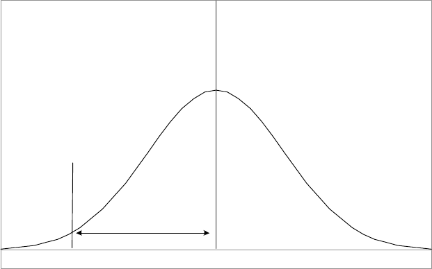
314 H. S. Bloom et al.
Average School
(50th percentile)
Weak School
(10th percentile)
τ
285.1
Figure 3. “Weak” and “average” schools in a local school performance distribution.
The variance of µ
j
is labeled τ
2
. It equals the variance across schools of
regression-adjusted mean test scores. This parameter represents the variance
of school performance holding constant selected student background charac-
teristics. Therefore τ represents the standard deviation of school performance
for students with similar backgrounds. It is this parameter that represents the
amount of variation that exists in school performance. Given an estimate of τ ,
it is possible to estimate the difference between the performance of the 10th
percentile school and the 50th percentile school in a district from the properties
of the normal curve.
Figure 3 illustrates how this can be done under the assumption that
school performance in a district is approximately normally distributed.
19
The
50th percentile score (for an average school) is located in the middle of
the school performance distribution. The 10th percentile score (for a weak
school) is located 1.285 school-level standard deviations (or 1.285 τ ) below
the 50th percentile score. This difference can be converted to an effect size
by dividing it by the standard deviation of test scores for all students in a
19
We compared results of the approach described here, which is based on the assump-
tion of normally distributed school performance, with an approach that uses the actual
residual for the schools that were located closest to the 10th and 50th percentiles in the
regression-adjusted performance distribution for each school district. Both approaches
yielded similar results, but we use the current approach because of its mathematical
clarity.
Downloaded by [Northwestern University] at 12:41 16 June 2014

Achievement Effect-Size Benchmarks 315
given grade from the district, which we label σ .
20
The resulting expression is
therefore
ES =
1.285τ
σ
(2)
For example, if τ were 10 scaled-score points, the difference in per-
formance levels between the 10th and 50th percentile schools would equal
1.285(10) or 12.85 scaled-score points. If σ were 30 scaled-score points, the
effect-size difference between the 10th and 50th percentile schools would be
(12.85/30) or 0.43 of a standard deviation. In this way performance gaps in
effect size can be computed for the two inferred points in the distribution of
school performance. These computations were made using multiple years of
data on standardized test scores in reading and math for Grades 3, 5, 7, and 10
from four large urban school districts.
21
Findings and Implications
Table 6 lists the resulting estimates of performance gaps, as effect sizes, between
weak and average schools in the four school districts for which data were
available.
22
The first panel reports findings for standardized tests of reading in
Grades 3, 5, 7 and 10; the second panel presents corresponding findings for
math.
Although these estimates vary across grades, districts, and academic sub-
ject, almost all of them lie between 0.20 and 0.40 of a student-level stan-
dard deviation. These findings have important implications for assessing the
effects of educational interventions that are assumed to potentially impact
the achievement of an entire school or, at least, an entire grade within a
school. For example, if an intervention were to improve student achieve-
ment by an effect size of 0.20—which would be deemed a “small effect”
20
This is the total student-level standard deviation for the district.
21
The standardized tests used are as follows: For District I, scaled scores from the
ITBS; for District II, scaled scores from the SAT9; for District III, normal curve equiv-
alent scores from the MAT; and for District IV, normal curve equivalent scores from the
SAT8.
22
The analysis in this section can be extended to compare other points in a normal
distribution of school performance by changing the multiplier in the numerator of
Equation 2. This multiplier indicates the number of school-level standard deviations
that lie between the two points in the distribution being compared. For example, the
effect size of the performance difference between the 10th and 90th percentile schools
in a district would have a multiplier of 2(1.285) or 2.57.
Downloaded by [Northwestern University] at 12:41 16 June 2014

316 H. S. Bloom et al.
Table 6 . Performance gap in effect size between “Average” and “Weak” schools (50th
and 10th percentiles)
District Findings
I II III IV
Reading
Grade 3 0.31 0.18 0.16 0.43
Grade 5 0.41 0.18 0.35 0.31
Grade 7 0.25 0.11 0.30 NA
Grade 10 0.07 0.11 NA NA
Math
Grade 3 0.29 0.25 0.19 0.41
Grade 5 0.27 0.23 0.36 0.26
Grade 7 0.20 0.15 0.23 NA
Grade 10 0.14 0.17 NA NA
Sources. ITBS for District I, SAT9 for District II, MAT for District III, and SAT8 for
District IV. See description in text for further details on the sample and calculations.
Note. “NA” indicates that a value could not be computed due to missing test
score data. Means are regression-adjusted for test scores in prior grade and students’
demographic characteristics.
according to Cohen’s default guidelines—it would be equivalent to closing
half to all of the performance gap between weak and average schools. When
viewed in this light, the intervention effect would seem to be anything but
small.
Another way to consider the same findings is to note that the difference
in mean student achievement between weak and average schools—which has
been deemed important enough to motivate many educational reforms—does
not look very large when viewed through the lens of effect size. Nevertheless,
enormous effort has been (and is being) expended to improve the performance
of weak schools. Any intervention that could raise their performance to the
level of average schools would be widely heralded as a major breakthrough.
This conclusion is consistent with that of Konstantopoulos and Hedges (2008)
from their analysis of data from a national sample of students and schools.
Both studies suggest that effect sizes that are much smaller than those previ-
ously thought to be necessary in order to be important might be highly policy
relevant.
It is important to be clear, however, that the effect size estimates for the
weak versus average school performance gaps reported here assume that the
students in the schools being compared have equal prior achievement scores
and background characteristics. This assumption focuses on school effects net
of variation across schools in the characteristics of their students. The actual
Downloaded by [Northwestern University] at 12:41 16 June 2014
Achievement Effect-Size Benchmarks 317
differences between schools with low mean achievement scores and those with
average mean scores, of course, represent contributions from factors associated
with the characteristics of the students enrolled in those schools as well as
factors associated with school effectiveness. The policy relevant performance
gaps associated with student characteristics are those we just discussed with
regard to differences among student subgroups. We have therefore viewed the
policy relevant performance gaps between schools in these analyses as those
associated only with school factors. Which of these gaps, or combinations of
gaps, are most relevant for interpreting an intervention effect size will depend
on the intent of the intervention and whether it primarily aims to change school
performance or student performance.
SUMMARY AND CONCLUSION
The research reported here is part of a larger project by the authors to de-
velop conceptual frameworks, analytic strategies, and empirical findings that
help researchers assess the substantive importance of the achievement effect
sizes produced by educational interventions. In this article we have explored
two complementary approaches to interpreting such effect sizes. The first fo-
cuses on the natural developmental progress on standardized achievement test
scores that occurs for students from year to year. Based on detailed information
for a set of nationally normed achievement tests, the academic developmen-
tal trajectory for average students in the United States appears to be one of
rapid growth in the first several grades of elementary school followed by grad-
ually declining gains in later grades. Expressed as effect sizes, the annual
gains in the early years are around 1.00, whereas those in the final grades of
high school are 0.20 or less. The pattern of these findings is strikingly similar
for all of the standardized tests and academic subjects examined. Their most
important implication for assessing effect sizes on such tests is that an inter-
vention effect of a given magnitude represents a much larger proportion of
normal annual growth for students in higher grades than it does for students in
lower grades.
The second approach explored in this article is comparison of interven-
tion effect sizes with the performance gaps for policy-relevant subgroups of
students or schools expressed in effect size terms. With respect to student sub-
groups, it was demonstrated that the gaps on standardized achievement tests
range from less than 0.10 of a standard deviation for gender differences in math
performance to almost a full standard deviation for race/ethnicity differences
in math and reading. Any given intervention effect size will therefore “look”
very different depending on the gap (or gaps) to which it is compared. With
respect to subgroups of schools, the difference between mean student achieve-
ment at weak schools (10th percentile) and average schools (50th percentile),
Downloaded by [Northwestern University] at 12:41 16 June 2014
318 H. S. Bloom et al.
expressed as student-level effect sizes, range from about 0.20 and 0.40. This
difference, which reflects only school factors and assumes students of simi-
lar ability and background, is still surprisingly small given the effort that has
been expended historically to improve the performance of weak schools. The
chief implication of this finding is that effect sizes for interventions aimed at
improving school performance could look small but still be large relative to
this gap.
In a companion article we will explore a third kind of empirical benchmark
for achievement effect sizes—distributions of effect sizes that have been found
in past research on the effects of educational interventions (Lipsey, Bloom,
Hill and Black, in preparation). A fourth approach is based on cost–benefit or
cost-effectiveness analysis to assess whether the value of the effects produced
by an intervention are sufficient to justify its costs or whether those costs are
more or less than those for alternative interventions that produce similar effects.
Work on this approach is outside the scope of this article but is being conducted
by others (e.g., Duncan & Magnuson, 2007; Harris, 2008; Ludwig & Phillips,
2007).
The full picture of approaches and considerations for assessing the practical
or substantive magnitude of achievement effect sizes for education interven-
tions is yet to be drawn and, no doubt, will continue to develop for many years to
come. Nonetheless, some general conclusions are already amply supported. The
most important of these, and the one least consistent with conventional practice,
is that there is no single, simple set of benchmarks for assessing the magnitude
of achievement effect sizes that is broadly applicable to education interven-
tions. Such interventions can be thought of as accelerating achievement gains,
closing policy relevant gaps, improving on the effects of prior interventions,
or seeking cost-effectiveness. They may target children in early, middle, or
later grades and address achievement in different academic subject areas. They
may aim to affect student performance directly or indirectly by improving the
effectiveness of teachers or schools. As seen in the analyses presented in this
article, all these variations potentially have somewhat different implications
for interpreting the practical or substantive magnitude of the corresponding
effect sizes.
In particular, Cohen’s widely used “small,” “medium,” and “large” effect
size heuristics and the sweeping claim that an effect size of 0.25 is required
for “educational significance” clearly have no general applicability to achieve-
ment effect sizes for educational interventions. Their one-size-fits-all charac-
ter is not sufficiently differentiated to be useful for any specific intervention
circumstance and is more likely to result in misleading expectations and in-
terpretations about the respective effect sizes. Cohen’s ubiquitous guidelines
are especially inappropriate for effect sizes on standardized achievement mea-
sures. His “medium” value of 0.50, viewed from the perspective of annual
achievement gains or policy relevant gaps, is not middling but huge—it would
Downloaded by [Northwestern University] at 12:41 16 June 2014
Achievement Effect-Size Benchmarks 319
close most of the gap between economically disadvantaged and advantaged
students, approximately double the annual achievement growth of children in
the middle grades, and make 10th percentile schools perform like 90th per-
centile ones. Even the more modest 0.25 effect size for alleged educational
significance has a poor fit with the annual gains of high school students and
school performance gaps, where it looks ambitious, and the annual gains of
early elementary students and student race/ethnic gaps, where it then looks less
impressive.
The variability in what seems like an effect size of meaningful magnitude
from different perspectives for different interventions in different circumstances
highlights another general conclusion that we believe the analyses presented
here support. Effect size benchmarks developed from national data may not
apply well to the local circumstances of any given intervention. We have mainly
used national data in this article to illustrate approaches to developing such
benchmarks, though we have also included a few instances of district-level
data. There is sufficient potential for differences that the wise course for an
intervention researcher is to use data from the context of the intervention to
apply any of the approaches discussed here if at all possible. If not possible,
we believe the empirical results we have presented applying those approaches
to national data and a few sets of local data provide better guidance than
the conventional Cohen guidelines and others of that ilk. Too little is known
about the extent of local variability, however, to be sure that any basis other
than relevant local data provides appropriate benchmarks for the effect sizes
associated with a given intervention.
Finally, we must emphasize that the empirical results presented here are
based on total subject matter scores for nationally normed standardized achieve-
ment tests. As such, those results may apply to similar tests used as intervention
outcomes but they do not necessarily apply to different measures of achieve-
ment. In particular, researchers often use more focused achievement tests or
subtests as outcome measures for educational interventions with which such
tests may be better aligned. For instance, a test of vocabulary or reading com-
prehension may be used rather than the total reading score on a comprehensive
achievement test, or a test of computation or geometry rather than a total math
score. Subject matter grades and grade point average are also sometimes used
as outcome measures and, occasionally, teacher ratings. We do not believe it
is safe to assume that the benchmarks applicable to such measures will be
similar to those for the broadband standardized achievement measures used in
the analyses presented in this article.
There is much work yet to be done if we are to have a good understanding
of how to assess the practical and substantive magnitude of the effect sizes
produced by educational interventions. We hope that by highlighting the con-
ceptual issues involved, promoting a multiperspective approach to assessing
effect sizes, and illustrating how to develop empirical benchmarks with real
Downloaded by [Northwestern University] at 12:41 16 June 2014
320 H. S. Bloom et al.
data, this article will help improve the design of future evaluations of educa-
tional interventions and the interpretation of their results.
ACKNOWLEDGMENTS
The research on which this article is based received support from the Institute
of Education Sciences in the U.S. Department of Education, the Judith Gueron
Fund at MDRC, and the William T. Grant Foundation. We thank Larry Hedges
for his helpful input.
REFERENCES
Bloom, H. S., Richburg-Hayes, L., & Black, A. R. (2007). Using covariates to improve
precision for studies that randomize schools to evaluate educational interventions.
Educational Evaluation and Policy Analysis, 29(1), 30–59.
Brennan, R. L. (2001). Generalizability theory. New York: Springer.
Cohen, J. (1988). Statistical power analysis for the behavioral sciences (2nd ed.).
Hillsdale, NJ: Erlbaum.
Cronbach, L. J., Gleser, G. C., Nanda H., & Rajaratnam, N. (1972). The dependability
of behavioral measurement: Theory of generalizability of scores and profiles.New
York: Wiley.
Duncan, G. J., & Magnuson, K. (2007). Penny wise and effect size foolish. Child
Development Perspectives, 1(1), 46–51.
Fisher, R. A. (1949). The design of experiments. Edinburgh, Scotland: Oliver &
Boyd.
Fleiss, J. L. (1994). Measures of effect size for categorical data. In H. Cooper & L.
V. Hedges (Eds.), The handbook of research synthesis (pp. 245–260). New York:
Russell Sage Foundation.
Fryer, R. G. Jr., & Levitt, S. D. (2006). The black-white test score gap through third
grade. American Law and Economics Review, 8(2), 249–281.
Glass, G. V., McGaw, B., & Smith, M. L. (1981). Meta-analysis in social research.
Beverly Hills, CA: Sage.
Grissom, R. J., & Kim, J. J. (2005). Effect sizes for research: A broad practical approach.
Mahwah, NJ: Erlbaum.
Harris, D. N. (2008, February 28). Toward new benchmarks for interpreting effect sizes:
Combining effects with costs (Working Paper). University of Wisconsin–Madison,
Madison, Wisconsin.
Hedges, L. V. (1982). Estimation of effect size from a series of independent experiments.
Psychological Bulletin, 92(2), 490–499.
Hedges, L. V., & Hedberg, E. C. (2007). Intra-class correlation values for planning
group-randomized trials in education. Educational Evaluation and Policy Analysis,
29(1), 60–87.
Hedges, L. V., & Olkin, I. (1985). Statistical methods for meta-analysis. Boston:
Academic.
Downloaded by [Northwestern University] at 12:41 16 June 2014
Achievement Effect-Size Benchmarks 321
Jencks, C., & Phillips, M. (1998). The black–white test score gap. Washington, DC:
Brookings Institution Press.
Kane, T. (2004). The impact of after-school programs: Interpreting the results of four
recent evaluations. New York: W. T. Grant Foundation.
Konstantopoulos, S., & Hedges, L. V. (2008). How large an effect can we expect from
school reforms? Teachers College Record, 110(8), 1613–1640.
Lipsey, M. W. (1990). Design sensitivity: Statistical power for experimental research.
Newbury Park, CA: Sage.
Lipsey, M. W., Bloom, H. S., Hill, C. J., & Black, A. R. (in preparation). Find-
ings from prior studies as achievement effect size benchmarks for educational
interventions.
Lipsey, M. W., & Wilson, D. B. (2001). Practical meta-analysis. Thousand Oaks, CA:
Sage.
Ludwig, J., & Phillips, D. A. (2007). The benefits and costs of head start. Society for
Research on Child Development, Social Policy Report, XXI(3), 3–18.
Neyman, J., & Pearson, E. S. (1928). On the use and interpretation of certain test
criteria for purposes of statistical inference. Biometrika, 20A, 175–240, 263–
294.
Neyman, J., & Pearson, E. S. (1933). On the Problem of the Most Efficient Tests of
Statistical Hypotheses. Philosophical Transactions of the Royal Society of London,
Ser. A, 231: 289–337.
Nunnally, J. C. (1967). Psychometric theory. New York: McGraw-Hill.
Rosenthal, R. (1991). Meta-analytic procedures for social science. Newbury Park, CA:
Sage.
Rosenthal, R. (1994). Parametric measures of effect size. In H. Cooper & L. V. Hedges
(Eds.), The handbook of research synthesis (pp. 231–244). New York: Russell Sage
Foundation.
Rosenthal, R., Rosnow, R. L., & Rubin, D. B. (2000). Contrasts and effect sizes in behav-
ioral research: A correlational approach. Cambridge, UK: Cambridge University
Press.
Shavelson, R. J., & Webb, N. M. (1991). Generalizability theory: A primer.Newbury
Park, CA: Sage.
Tallmadge, G. K. (1977). The joint dissemination review panel IDEABOOK. Washing-
ton, DC: U. S. Office of Education.
TerraNova, The Second Edition (2002). California Achievement Tests, Technical
Report I (Monterey, CA: CTB/McGraw-Hill).
APPENDIX A: STANDARD DEVIATIONS OF SCALED SCORES
Table A1 shows that for each test, standard deviations are stable across grades
K-12. Thus, effect size patterns reported in this paper are determined almost
entirely by differences among grades in mean scaled scores. In other words,
it is the variation in growth of measured student achievement across grades
K-12 that produces the reported pattern of grade-to-grade effect sizes—not
differences in standard deviations across grades.
Downloaded by [Northwestern University] at 12:41 16 June 2014

322 H. S. Bloom et al.
Table A1. Reading: Standard deviations of scale scores by grade for each test
Terra Nova- Gates- Terra Nova-
G rade C AT5 S AT9 CTB S M acG init ie M AT8 C AT SAT1 0
Kindergarden 47.4 38.5 . 38.2 46.6 . 41.7
1st 45.4 45.4 42.2 47.4 51.6 44.6 47.3
2nd 45.1 41.3 40.8 43.2 48.6 43.1 42.2
3rd 42.5 43.3 41.1 39.3 40.4 40.6 38.1
4th 43.0 44.1 42.5 38.3 40.3 41.2 39.2
5th 40.2 39.1 38.5 34.8 39.7 40.7 36.7
6th 41.5 38.1 40.3 35.4 36.7 41.7 37.3
7th 42.0 38.6 39.9 32.6 36.7 42.0 39.1
8th 42.3 40.1 39.9 34.3 35.2 42.1 37.3
9th 43.3 38.9 38.7 35.8 38.1 41.9 37.4
10th 42.4 36.7 40.4 34.3 36.7 43.6 35.6
11th 43.8 35.9 40.9 34.3 37.7 45.1 43.0
12th 46.2 36.5 42.1 36.2 36.3 45.6 45.3
Sources. CAT5 (1991 norming sample): CTB/McGraw-Hill. 1996. CAT5: Techni-
cal Report. (Monterey, CA: CTB/McGraw-Hill), pp. 308–311. SAT9 (1995 norming
sample); from Harcourt-Brace Educational Measurement. 1997. Stanford Achieve-
ment Test Series, 9th edition: Technical Data Report (San Antonio: Harcourt), Tables
N-1 and N-4 (for SESAT), N-2 and N-5 (SAT) and N-3 and N-6 (for TASK). Terra
Nova-CTBS (1996 norming sample): CTB/McGraw-Hill. 2001. TerraNova Compre-
hensive Test of Basic Skills (CTBS) Technical Report. (Monterey, CA: CTB/McGraw-
Hill), pp. 361–366. Gates-MacGinitie (1998–1999 norming sample): MacGinitie,
Walter H. et al. 2002. Gates-MacGinitie Reading Tests, Technical Rep ort (Forms S and
T), Fourth Edition. (Itasca, IL: Riverside Publishing), p. 57. MAT8 (1999–2000 norm-
ing sample) from Harcourt Educational Measurement. Metropolitan8: Metropolitan
Achievement Tests, Eighth Edition (Harcourt), pp. 264–269. Terra Nova-CAT (1999–
2000 norming sample): CTB/McGraw-Hill. 2002. TerraNova, The Second Edition:
California Achievement Tests, Technical Report 1. (Monterey, CA: CTB/McGraw-
Hill), pp. 237–242. SAT10 (2002 norming sample): Stanford Achievement Test Series:
Tenth Edition: Technical Data Report. 2004. (Harcourt Assessment) pp. 312–338.
Note. For each test, spring standard deviations are shown. For the SAT9 and SAT10,
9th graders took both the SAT and TASK versions so the standard deviation above
pools together data from both tests. The Kindergarden standard deviation is missing
for the Terra Nova-CTBS and Terra Nova-CAT because a “Vocabulary” component
was not included in Level 10 administered to K students. This component is included
in the Reading Composite for all other grade levels.
APPENDIX B
Variance of the Difference Between Cross-Sectional and Longitudinal
Differences of Means
1. Difference between the two estimators
X
= (
¯
X
1A
−
¯
X
2B
) − (
¯
X
∗
1A
−
¯
X
∗
2A
) = difference in estimators
Downloaded by [Northwestern University] at 12:41 16 June 2014
Achievement Effect-Size Benchmarks 323
¯
X
1A
= mean outcome for full first-grade sample
¯
X
2B
= mean outcome for second-grade sample the same year
¯
X
∗
1A
= mean first-grade outcome for the longitudinal subsample
¯
X
∗
2A
= mean second-grade outcome for the longitudinal sample (in the
second year)
2. Variance of the Difference
Var(
X
) = Var(
¯
X
1A
) + Var(
¯
X
2B
) + Var(
¯
X
∗
1A
) + Var(
¯
X
∗
2A
)
−2Cov(
¯
X
1A
,
¯
X
2B
) − 2Cov(
¯
X
1A
,
¯
X
∗
1A
) + 2Cov(
¯
X
1A
,
¯
X
∗
2A
)(3)
+2Cov(
¯
X
2B
,
¯
X
∗
1A
) − 2Cov(
¯
X
2B
,
¯
X
∗
2A
) − 2Cov(
¯
X
∗
1A
,
¯
X
∗
2A
)
3. Define each Covariance
Cov(
¯
X
1A
,
¯
X
2B
) = 0 (independent samples)
Cov(
¯
X
1A
,
¯
X
∗
1A
) = wV ar(
¯
X
∗
1A
) (partly-overlapping samples at the same
time; proof below)
Cov(
¯
X
1A
,
¯
X
∗
2A
) = wρ V ar (
¯
X
∗
1A
)(partly-overlapping samples one year
apart; proof below)
Cov(
¯
X
2B
,
¯
X
∗
1A
) = 0 (independent samples)
Cov(
¯
X
2B
,
¯
X
∗
2A
) = 0 (independent samples)
Cov(
¯
X
∗
1A
,
¯
X
∗
2A
) = ρV ar(
¯
X
∗
1A
) (same sample one year apart; proof below)
4. Obtaining the Covariance for Partly Overlapping Samples
at Same Time
r
Express the full-group mean as a weighted sum of those who remain in
the longitudinal sample, and those who do not:
¯
X
1A
= w
¯
X
∗
1A
+ (1 − w)
¯
X
1C
where
w = the proportion of the full first-grade sample that is also in the
longitudinal analysis
¯
X
1C
=the mean first-grade score for the non-overlapping part of the
first-grade sample
Downloaded by [Northwestern University] at 12:41 16 June 2014
324 H. S. Bloom et al.
r
Then:
Cov(
¯
X
1A
,
¯
X
∗
1A
) = Cov[(w
¯
X
∗
1A
+ (1 − w)
¯
X
1C
),
¯
X
∗
1A
]
= Cov[w
¯
X
∗
1A
,
¯
X
∗
1A
]
= wV ar(
¯
X
∗
1A
)
5. Covariance for Partly-Overlapping Sample One Year Apart
r
Express the second-year score for student i as a function of the first-year
score plus random error:
X
2i
= ρX
1i
+ ν
i
where
w = the proportion of the full first-grade sample that is also in the
longitudinal analysis
ρ = year-to-year correlation in outcomes
ν
i
= random error
r
Then
¯
X
1A
= w
¯
X
∗
1A
+ (1 − w)
¯
X
1C
¯
X
∗
2A
= ρ
¯
X
∗
1A
+ ¯ν
2A
Cov(
¯
X
1A
,
¯
X
∗
2A
) = Cov
[w
¯
X
∗
1A
+ (1 − w)
¯
X
1C
], [ρ
¯
X
∗
1A
+ ¯ν
2A
]
= Cov(w
¯
X
∗
1A
,ρ
¯
X
∗
1A
) + Cov(w
¯
X
∗
1A
, ¯ν
2A
)
+Cov[(1 − w)
¯
X
1C
,ρ
¯
X
∗
1A
] + Cov[(1 − w)
¯
X
1C
, ¯ν
2A
]
= wρV ar (
¯
X
∗
1A
) + 0 +0 + 0
= wρV ar (
¯
X
∗
1A
)
6. Covariance for t he Longitudinal Sample Across Two Years
Cov(
¯
X
∗
1A
,
¯
X
∗
2A
) = Cov
(
¯
X
∗
1A
), (ρ
¯
X
∗
1A
+ ¯ν
2A
)
= Cov(
¯
X
∗
1A
,ρ
¯
X
∗
1A
) + Cov(
¯
X
∗
1A
, ¯ν
2A
)
= ρV ar(
¯
X
∗
1A
) + 0
= ρV ar(
¯
X
∗
1A
)
Downloaded by [Northwestern University] at 12:41 16 June 2014
Achievement Effect-Size Benchmarks 325
7. Substitute all terms for Covariances back into Expression [1]
Var(
X
) = Var(
¯
X
1A
) + Var(
¯
X
2B
) + Var(
¯
X
∗
1A
) + Var(
¯
X
∗
2A
)
−2Cov(
¯
X
1A
,
¯
X
2B
) − 2Cov(
¯
X
1A
,
¯
X
∗
1A
) + 2Cov(
¯
X
1A
,
¯
X
∗
2A
)
+2Cov(
¯
X
2B
,
¯
X
∗
1A
) − 2Cov(
¯
X
2B
,
¯
X
∗
2A
) − 2Cov(
¯
X
∗
1A
,
¯
X
∗
2A
)
= Var(
¯
X
1A
) + Var(
¯
X
2B
) + Var(
¯
X
∗
1A
) + Var(
¯
X
∗
2A
)
−0 − 2wV ar(
¯
X
∗
1A
) + 2wρ V ar (
¯
X
∗
1A
)
+0 − 0 −2ρV ar(
¯
X
∗
1A
)
= Var(
¯
X
1A
) + Var(
¯
X
2B
) + (1 −2w + 2wρ − 2ρ)Var(
¯
X
∗
1A
)
+Var(
¯
X
∗
2A
)
8. Check: What happens if the Samples are Fully-Overlapping (i.e., w=1
and
¯
X
1A
=
¯
X
∗
1A
):
From the definition of the difference:
Var(
X
) = Var[(
¯
X
1A
−
¯
X
2B
) − (
¯
X
∗
1A
−
¯
X
∗
2A
)]
= Var[
¯
X
∗
1A
−
¯
X
2B
) − (
¯
X
∗
1A
−
¯
X
∗
2A
)]
= Var(
¯
X
∗
2A
−
¯
X
2B
)
= Var(
¯
X
∗
2A
) + Var(
¯
X
2B
) − 2Cov(
¯
X
∗
2A
,
¯
X
2B
)
= Var(
¯
X
∗
2A
) + Var(
¯
X
2B
)
From the derived formula:
Var(
X
) = Var(
¯
X
1A
) + Var(
¯
X
2B
) + (1 −2w + 2wρ − 2ρ)Var(
¯
X
∗
1A
)
+Var(
¯
X
∗
2A
)
= Var(
¯
X
∗
1A
) + Var(
¯
X
2B
) + [1 −2 + 2ρ − 2ρ]Var(
¯
X
∗
1A
)
+Var(
¯
X
∗
2A
)
= Var(
¯
X
2B
) + Var(
¯
X
∗
2A
)
→CHECKS OUT AS IT SHOULD.
Downloaded by [Northwestern University] at 12:41 16 June 2014

326 H. S. Bloom et al.
APPENDIX C
Developmental Trajectories Across Tests Within Multiple Subjects
Tables C1, C2, and C3 show that similar developmental trajectories exist across
specific tests within all four subjects—average annual growth tends to decrease
at a decreasing rate as students move from early grades to later grades.
Table C1. Annual math gain in effect size from six nationally-normed tests
Grade Terra Nova Terra Nova Mean for Margin of
Transition CAT5 SAT9 CTBS MAT8 CAT SAT10 the Six Tests Error (95%)
Grade K –1 . 1.07 . 1.36 . 1.00 1.14 ± 0.49
Grade 1 – 2 1.09 1.04 1.14 0.85 0.91 1.17 1.03 ± 0.14
Grade 2 – 3 0.78 0.74 1.05 0.81 1.18 0.78 0.89 ± 0.16
Grade 3 – 4 0.52 0.63 0.62 0.44 0.60 0.28 0.52 ± 0.14
Grade 4 – 5 0.72 0.59 0.53 0.49 0.47 0.58 0.56 ± 0.11
Grade 5 – 6 0.42 0.30 0.46 0.34 0.47 0.48 0.41 ± 0.08
Grade 6 – 7 0.29 0.38 0.31 0.34 0.18 0.28 0.30 ± 0.06
Grade 7 – 8 0.32 0.28 0.34 0.25 0.39 0.32 0.32 ± 0.05
Grade 8 – 9 0.15 0.15 0.20 0.32 0.15 0.33 0.22 ± 0.10
Grade 9 –10 0.22 0.34 0.23 0.16 0.22 0.31 0.25 ± 0.07
Grade 10 –11 0.26 −0.09 0.26 −0.05 0.26 0.18 0.14 ± 0.16
Grade 11 –12 0.13 −0.10 0.11 −0.06 0.12 −0.13 0.01 ± 0.14
Sources. CAT5 (1991 norming sample): CTB/McGraw-Hill. 1996. CAT5: Techni-
cal Report. (Monterey, CA: CTB/McGraw-Hill), pp. 308–311. SAT9 (1995 norming
sample): Harcourt-Brace Educational Measurement. 1997. Stanford Achievement Test
Series, 9th edition: Technical Data Report (San Antonio: Harcourt), Tables N-1 and N-4
(for SESAT), N-2 and N-5 (SAT) and N-3 and N-6 (for TASK). Terra Nova-CTBS (19
96 norming sample): CTB/McGraw-Hill. 2001. TerraNova Comprehensive Test of Ba-
sic Skills (CTBS) Technical Report. (Monterey, CA: CTB/McGraw-Hill), pp. 361–366.
MAT8 (1999–2000 norming sample): Harcourt Educational Measurement. Metropoli-
tan8: Metropolitan Achievement Tests, Eighth Edition (Harcourt), pp. 264–269. Terra
Nova-CAT (1999–2000 norming sample): CTB/McGraw-Hill. 2002. TerraNova, The
Second Edition: California Achievement Tests, Technical Report 1. (Monterey, CA:
CTB/McGraw-Hill), pp. 237–242. SAT10 (2002 norming sample): Stanford Achieve-
ment Test Series: Tenth Edition: Technical Data Report. 2004. (Harcourt Assessment)
pp. 312–338.
Note. Spring-to-spring differences are shown. The mean is calculated as the weighted
mean of the six effect sizes (three for the K-1 transition). 95% CI are computed using
critical values for the t-distribution with 2 d.f. for the K-1 transition and 5 d.f. for all
other transitions. The K-1 transition is missing for the Terra Nova-CTBS and Terra
Nova-CAT, because a “Mathematics Computation” component was not included in
Level 10 of the test administered to K students. This component is included in all other
levels of the Math Composite score.
Downloaded by [Northwestern University] at 12:41 16 June 2014

Achievement Effect-Size Benchmarks 327
Table C2. Annual science gain in effect size from six nationally-normed tests
Grade Terra Nova Terra Nova Mean for Margin of
Transition CAT5 SAT9 CTBS MAT8 CAT SAT10 the Six Tests Error (95%)
Grade K – 1 . . . . . . . .
Grade 1 – 2 0.76 . 0.57 0.52 0.45 . 0.58 ± 0.24
Grade 2 – 3 0.49 . 0.43 0.49 0.50 . 0.48 ± 0.04
Grade 3 – 4 0.33 0.46 0.43 0.40 0.50 0.09 0.37 ± 0.16
Grade 4 – 5 0.51 0.34 0.39 0.43 0.36 0.36 0.40 ± 0.08
Grade 5 – 6 0.28 0.18 0.23 0.23 0.27 0.44 0.27 ± 0.10
Grade 6 – 7 0.22 0.27 0.32 0.34 0.29 0.23 0.28 ± 0.05
Grade 7 –8 0.15 0.35 0.25 0.22 0.26 0.31 0.26 ± 0.09
Grade 8 – 9 0.19 0.25 0.11 0.37 0.09 0.28 0.22 ± 0.10
Grade 9 – 10 0.18 0.18 0.20 0.04 0.15 0.36 0.19 ± 0.11
Grade 10 – 11 0.28 0.11 0.33 −0.22 0.27 0.12 0.15 ± 0.18
Grade 11 – 12 0.08 −0.01 0.07 0.07 0.14 −0.12 0.04 ± 0.12
Sources. CAT5 (1991 norming sample): CTB/McGraw-Hill. 1996. CAT5: Technical
Report. (Monterey, CA: CTB/McGraw-Hill), pp. 308–311. SAT9(1995 norming sam-
ple); from Harcourt-Brace Educational Measurement. 1997. Stanford Achievement Test
Series, 9th edition: Technical Data Report (San Antonio: Harcourt), Tables N-1 and N-4
(for SESAT), N-2 and N-5 (SAT)and N-3 and N-6 (for TASK). Terra Nova-CTBS (1996
norming sample): CTB/McGraw-Hill. 2001. TerraNova Comprehensive Test of Basic
Skills (CTBS) Technical Report. (Monterey, CA: CTB/McGraw-Hill), pp. 361-366.
Gates-MacGinitie (1998–1999 norming sample): MacGinitie, Walter H. et al. 2002.
Gates-MacGinitie Reading Tests, Technical Report (Forms S and T), Fourth Edi-
tion. (Itasca, IL: Riverside Publishing), p. 57. MAT8 (1999–2000 norming sample)
from Harcourt Educational Measurement. Metropolitan8: Metropolitan Achievement
Tests, Eighth Edition (Harcourt), pp. 264–269. Terra Nova-CAT (1999–2000 norm-
ing sample): CTB/McGraw-Hill. 2002. TerraNova, The Second Edition: California
Achievement Tests, Technical Report 1. (Monterey, CA: CTB/McGraw-Hill), pp. 237–
242. SAT10 (2002 norming sample): Stanford Achievement Test Series: Tenth Edition:
Technical Data Report. 2004. (Harcourt Assessment) pp. 312–338.
Note. Spring-to-spring differences are shown. The mean is calculated as the weighted
mean of the six effect sizes (four each for the 1-2 and 2-3 transition). 95% CI are com-
puted using critical values for the t -distribution with 3 d.f. for the 1-2 and 2-3 transitions
and 5 d.f. for all other transitions.
Downloaded by [Northwestern University] at 12:41 16 June 2014

328 H. S. Bloom et al.
Table C3. Annual social studies gain in effect size from six nationally-normed tests
Grade Terra Nova Terra Nova Mean for Margin of
Transition CAT5 SAT9 CTBS MAT8 CAT SAT10 the Six Tests Error (95%)
Grade K –1 . . . . . . . .
Grade 1 –2 0.61 . 0.58 0.73 0.59 . 0.63 ± 0.11
Grade 2 –3 0.49 . 0.45 0.67 0.44 . 0.51 ± 0.17
Grade 3 – 4 0.33 0.33 0.32 0.38 0.46 0.18 0.33 ± 0.10
Grade 4 – 5 0.42 0.38 0.30 0.45 0.22 0.33 0.35 ± 0.08
Grade 5 – 6 0.31 0.40 0.30 0.22 0.24 0.43 0.32 ± 0.09
Grade 6 – 7 0.07 0.30 0.23 0.35 0.34 0.33 0.27 ± 0.14
Grade 7 – 8 0.29 0.26 0.15 0.32 0.16 0.27 0.25 ± 0.06
Grade 8 – 9 0.12 0.25 0.16 0.22 0.14 0.21 0.18 ± 0.06
Grade 9 –10 0.11 0.21 0.18 0.12 0.19 0.31 0.19 ± 0.09
Grade 10 –11 0.18 0.07 0.38 −0.25 0.37 0.16 0.15 ± 0.19
Grade 11 –12 0.11 −0.20 0.15 0.10 0.19 −0.08 0.04 ± 0.16
Sources. CAT5 (1991 norming sample): CTB/McGraw-Hill. 1996. CAT5: Techni-
cal Report. (Monterey, CA: CTB/McGraw-Hill), pp. 308–311. SAT9 (1995 norming
sample): Harcourt-Brace Educational Measurement. 1997. Stanford Achievement Test
Series, 9th edition: Technical Data Report (San Antonio: Harcourt), Tables N-1 and N-4
(for SESAT), N-2 and N-5 (SAT) and N-3 and N-6 (for TASK). Terra Nova-CTBS (19
96 norming sample): CTB/McGraw-Hill. 2001. TerraNova Comprehensive Test of Ba-
sic Skills (CTBS) Technical Report. (Monterey, CA: CTB/McGraw-Hill), pp. 361–366.
MAT8 (1999–2000 norming sample): Harcourt Educational Measurement. Metropoli-
tan8: Metropolitan Achievement Tests, Eighth Edition (Harcourt), pp. 264–269. Terra
Nova-CAT (1999–2000 norming sample): CTB/McGraw-Hill. 2002. TerraNova, The
Second Edition: California Achievement Tests, Technical Report 1. (Monterey, CA:
CTB/McGraw-Hill), pp. 237–242. SAT10 (2002 norming sample): Stanford Achieve-
ment Test Series: Tenth Edition: Technical Data Report. 2004. (Harcourt Assessment)
pp. 312–338.
Note. Spring-to-spring differences are shown. The mean is calculated as the weighted
mean of the six effect sizes (four each for the 1-2 and 2-3 transition). 95% CI are com-
puted using critical values for the t-distribution with 3 d.f. for the 1-2 and 2-3 transition
and 5 d.f. for all other transitions.
Downloaded by [Northwestern University] at 12:41 16 June 2014
