Predictive Modeling for Real Estate Days on Market

Utah State University Utah State University

DigitalCommons@USU DigitalCommons@USU

All Graduate Plan B and other Reports Graduate Studies

5-2021

Predictive Modeling for Real Estate Days on Market Predictive Modeling for Real Estate Days on Market

Jeffrey Brann

Utah State University

Follow this and additional works at: https://digitalcommons.usu.edu/gradreports

Part of the Real Estate Commons

Recommended Citation Recommended Citation

Brann, Jeffrey, "Predictive Modeling for Real Estate Days on Market" (2021).

All Graduate Plan B and other

Reports

. 1537.

https://digitalcommons.usu.edu/gradreports/1537

This Creative Project is brought to you for free and open

access by the Graduate Studies at

DigitalCommons@USU. It has been accepted for

inclusion in All Graduate Plan B and other Reports by an

authorized administrator of DigitalCommons@USU. For

more information, please contact

[email protected].

Predictive Modeling for Real Estate Days on Market

Jeffrey Brann

Abstract

Many forms of property valuation exist but estimation models for duration on market are not

as common. This Paper examines a variety of variables as well those that would be found in a

hedonistic valuation model and applies them to a predictive model estimating a property’s

duration on market. A brief real estate market analysis is also provided regarding Cache

County, Utah to give better clarity as to the environment in which this predictive model is

performing.

Keywords: Real Estate, Single Family Homes, Predictive Modeling

Introduction

How much is my home worth? How quickly can I sell? These are questions that almost

all homeowners face at some point in their lives. As individuals decide to move out of their

starter homes, seek to relocate long term, or even downsize later in life, they will most likely

attempt to sell a property. While there are many ways to predict the value of a property, the

most common way of predicting time on market is to look at a historical average. This paper

looks deeper into estimating the time that a property will remain on market before it is under

contract. This estimation benefits the seller by allowing them to set realistic expectations for

the sale of their property, plan for costs of holding, and have a timeframe for possibly entering

another property. It can also be a signal to buyers regarding the popularity of a property,

especially if it has been on market longer than typical properties in the area (Zhu, Xiong, Tang,

Liu, Ge, Chen, Fu, 2016).

The focus of this study is looking at single family properties sold in Cache County, Utah

between January 2010 and December 2020. The state of Utah provides some unique metrics

when considering this study. Over the 10-year span studied for this paper, Utah remains in the

top 4 states with greatest appreciation. Utah has been consistently growing and new

companies are moving in every year. Cache County itself stays a little lower than state average

for appreciation but still experiences rapid growth (Change, 2020). Because it is home to Utah

State University, there are some other unique attributes to the real estate market of Cache

County; for example, there are many parents that buy houses for their children to live in while

attending school then plan to sell them for a profit after graduation. Investors also buy many

properties around the university, as there is a steady supply of tenants potentially allowing the

investor to hold a cash-flowing property. On top of this there are the long-term residents of

the valley that are purchasing properties as a primary residence be it students who decided to

stay in the valley after graduation, families and individuals that are just part of the growing

population, or employees that are part of the growing local industry.

All in all, Cache County has had what is referred to as a “hot” or sellers’ market for the

last few years, meaning houses sell quickly on the market, often close to the asking price. Of all

properties that were part of this study, about 22% of them sold for a premium (paid more than

was asked) with the majority of this coming into play from 2015 to 2020. Sellers’ markets are

marked by lower inventory than demand, leading to potential bidding wars which can lead to

said premium in many cases (Taylor, 1995). All of this leads to a very dynamic and active real

estate market in Cache County.

Data Description

The data collected for this study comes from utahrealestate.com, which is the multiple

listing service (MLS) for all of Utah with the exception of two cities. Parameters were single

family homes that were listed and sold in Cache County Utah between January 1, 2010 and

December 31, 2020. Price range was restricted to being between $100,000 and $600,000 to

capture single family homes that most consumers in the area would be looking for. While

smaller and larger properties are available, houses in that price range cater to a more specific

market. To provide a more accurate measure of available inventory, listings that were

cancelled were also included but were not analyzed due to a lack of under-contract date,

meaning they were counted as available inventory but nothing else. Having the under-contract

data is imperative as the basic valuation of days on market is calculated from under-contract

date minus the entry date.

The time frame of the data does include some large impacting events. Since the data

begins in 2010, the recovery from the 2008 market crash is captured and an increase of positive

market sentimentality can be detected. The average mortgage interest rate stayed consistent

around 3.5% and 4.5% from 2010 to 2019 and therefore was not considered a large factor for

this study (Ceizyk, 2021). The latter end of the data captures some of the beginning effects of

the COVID-19 pandemic that shook financial markets from March 2020 until the end of the

year. One of the major impacts of the virus that this paper can observe is the decrease in

federal interest rates and subsequently a large decrease of mortgage interest rates. While the

purpose of this paper is not to provide an all-inclusive examination of the effects of the virus on

the local real estate market, it is an interesting factor. Total impact may not be seen for years

to come with many indirect influences on the market. Further research will be required to

examine the full extent of the COVID-19 pandemic and the impact it caused on housing

markets.

Another key component that is not investigated in this paper is the impact of new

construction. This is a large factor for the overall market but due to the data sample there is

not enough information on new construction to provide clear insight on its impact. On-market

data does not always include the full story in the situation of new construction. Homes that are

built on lots that have been already purchased by the owner and negotiated with a contractor

never get listed on the for-sale market. Developers that are building subdivisions may only list

a few of the model homes but not every property in the subdivision. This would have been an

important variable to consider as the proximity to new construction changes values of nearby

properties, inventory of available houses, and is a good indicator of positive market sentiment

(Zahirovich and Gibler, 2014).

After removing data points that were missing critical variables, a total of 12,873

properties were observed. The dependent variable that this paper is studying is days on market

(DOM). This is derived from the difference between the listing date of the property and the

date it goes under contract with the closing buyers. Variables that were included in this study

included those that would be found in a hedonic model, or a model that breaks a house down

into its key parts, such as original listing price, total number bedrooms, bathrooms, and square

footage (Sirmans, Macpherson, & Zietz 2005). Square footage is measured in hundreds of

square feet. Age of the property was also included and for simplicity’s sake, expressed as a

variable of entry year minus year built. For example, a property built in 2005 and sold in 2015

would be calculated as 2015-2005= 10 or age = 10. Age of 0 indicates the property was built in

year that it was sold. Houses that sold higher than original asking price would be considered

selling on premium and have been included as dummy or categorical variable that has been

broken down into positive quartiles. Houses not selling for a premium or at asking price were

marked as a zero (0). A one (1) indicates selling up to .89% over listing price, two (2) is up to

1.86%, three (3) is up to 3.33%, and four (4) up to 74.47%. Timing of the transaction was also

accounted for in this study as dummy variables for the year and month. Base variables for

month and year are respectively April and 2010. Additionally, because he COVID-19 pandemic

started to have an economic impact in Cache County in early 2020, to capture this specific

impact another dummy variable was included that takes into consideration whether the

transaction took place during the COVID-19 pandemic, specifically from March 1, 2020 to

December 31, 2020. This Covid variable accounts for 1216 properties sold. Last of all, the

binary dummy variable InvAve was created to indicate if inventory at the time of listing was

above annual average -- noted with a 1 -- or below annual average -- noted as 0. Natural

logarithms were used for the dependent variable to correct for skewness as well as original

listing price to help with interpretation. All variables and their descriptions are listed in Table 1.

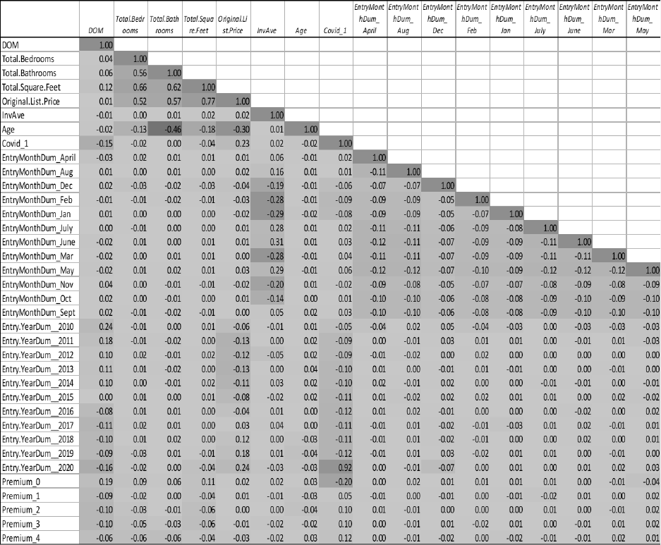
Correlations between all variables are found in Table 2. High correlation is observed

and expected between bedrooms, bathrooms, and square footage. Larger houses generally

have more rooms such as bedrooms and bathrooms with a 2:1 ratio. Older houses did not

follow this ratio as often, which explains why age has a high negative correlation with

bathrooms. The newer a house is the more likely it follows the 2:1 bedroom-to-bathroom ratio.

High correlation also exists between the dummy variable for 2020 and Covid. This is also

expected as 2020 only incorporates 3 additional months than the Covid variable. Last of all,

high correlation exists between the premium0 variable and the other premium variables.

Houses either do not sell on premium or they sell within one of the quartiles. This almost

binary condition leads to the high correlation.

Statistical Summaries

Table 3 includes summary statistics for discrete variables. The average house in this

study was a 4-bedroom, 2-bathroom house with about 2,300 square feet. Average time on

market was about two months with a listing price of $230,000. For any house sold there would

typically be another 385 properties to choose from in the valley. Table 4 provides a snapshot of

transactional behaviors for the ten years that are included in this study. Note that Premium

Percent of Total is for the given year and Average Inventory is the average number of houses

available per every sale. The general trend of increasing house sales can be observed from

2010 all the way through 2020; in contrast, DOM trends downward throughout the decade.

General property value appreciation can also be observed as properties listed on average were

about $195,000 in 2010 and $294,000 by 2020. A point of interest would also be the increase

of houses selling on premium to the point where 46% of houses sold in 2020 sold on premium,

as opposed to a mere %5 that sold on premium in 2010.

Empirical Tests and Results

For this study, a regression model was created using the order of least squares method

and combined elements from other studies to determine variables. The true model is as

follows:

Ln(DOM)

= ϐ

+ ϐ

Ln(ListPrice

)

+ ϐ

Age

+ ϐ

TotalBedrooms

+ ϐ

TotalBathrooms

+ ϐ

Sqrft

Year2011

+ ϐ

Year2012

+ ϐ

Year2013

+ ϐ

Year2014

+ ϐ

Year2015

+ ϐ

Year2016

Year2017

+ ϐ

Year2018

+ ϐ

Year2019

+ ϐ

Year2020

+ ϐ

MonthJan

+ ϐ

MonthFeb

Mar

+ ϐ

MonthMay

+ ϐ

MonthJune

+ϐ

MonthJuly

+ ϐ

MonthAug

+ ϐ

MonthSept

MonthOct

+ ϐ

MonthNov

+ ϐ

MonthDec

+ϐ

Covid

+ ϐ

Premium1

+ ϐ

Premium2

Premium3

+ ϐ

Premium4

+ ϐ

InvAve

+ ε

Due to heteroscedasticity found in the base model, the estimated model uses robust standard

error. A logarithmic model was used due to the skewness present in the DOM variables, given

that the majority of the observations are clustered to the left side, or less days on market. The

estimated coefficients and their significance are found in Table 5. Note lack of major

significance for total bathrooms which would be explained by the higher correlation with

bedrooms and square footage. The months of May, June, and July are not noted as significant

in this model as well as the Covid variable. Covid would be explained by high correlation with

the year 2020 variable. Insignificant variables were included in the model as they do contribute

to a higher R

value, meaning they do help explain the variance in the model. All other variables

are significant with 99% confidence.

The estimated model indicates that for every percent increase of price, time on market

will increase by 0.321%. For every year older that a house is, there will be a decrease of 0.1% of

time on market. For every bedroom included in a property, time on market decreases by 7%.

For every 100 square feet, DOM increases 1.4%. Every year after 2010 decreased time on

market compared to 2010. DOM in 2011 decrease by 56.3% in comparison to 2010; similarly,

2012 decreased by 76.3%, 2013 by 78.2%, 2014 by 82.8%, 2015 by 122.0%, 2016 by 164.1%,

2017 by 183.7%, 2018 by 177.3%, 2019 by 172.8%, and 2020 decreased DOM by 196.3%. All

months that held significance increased time on market as compared to April. Compared to

April, for example, January increased DOM by 40.7%, February by 20.2%, March by 14.1%,

August by 22.3%, September by 18.8%, October by 30.9%, November by 36% and December by

34.9%. The positive premium quartiles all decreased time on market compared to those houses

that sold at asking price or less. Quartile 1 or Premium1 decreases DOM by 68.7%, Premium2

by 81.3%, Premium3 by 82.7%, and Premium4 by 71.6%. The InvAve variable indicates an

increase of DOM of 12.4% when compared to those houses that sold below annual average

inventory. Caution should be exercise for interpreting the coefficients for bathrooms, May,

June, July, and Covid due to lack of significance.

The relationship between the InvAve and premium would have been expected that

lower than average inventory would result in more premiums being paid, but this was not

observed consistently through this study. Table 6 provides a breakdown of premiums paid

compared to inventory averages on a year-to-year basis. Basic supply and demand theory

would indicate that lower inventory (less supply) would be paired with more demand or

premiums paid. While this was the case for 2015 and 2020 it is not seen in the rest of the data.

A possible explanation for this seemingly counterintuitive result would be that the overall

inventory, regardless of annual averages, was below the demand levels resulting in premium

being paid even when inventory was above the annual average.

It was unsure how the COVID-19 pandemic would impact real estate but at least in 2020

it did not have a negative impact on DOM. The reduced federal interest rate resulting in low

mortgage rates would be a factor for the decrease seen in the Covid variable as well of the

implications that there was still a large demand for housing paired with decreasing inventory. It

would be expected that with the decreased inventory, 2020 would have had more time on

market as it had less inventory than the previous two years. As mentioned however, there was

no indication of decreased demand and 2020 still had faster sales than the year previous.

Another consideration that could factor into this decrease was the stimulus checks that were

sent out to the American people from the federal government encouraging them to consume

more. As mentioned before though, drawing conclusions on the impact of the pandemic may

still be premature. While the Covid variable is insignificant and the 2020 variable seems to

capture the majority of the impact, it is also possible that they are reflecting the impact of other

variables that were not captured in this model.

The adjusted R

of this model is 0.259, meaning the independent variables of this model

account for 25.9% of the variance found in days on market. As mentioned before, variables

such as new construction were not included as well as many other variables which would have

produced a better fitting model. As real estate purchasing is a multifaceted process with many

contributing factors, getting a perfectly fitted model is not very probable.

Conclusion

Most variables in this study’s model reduce the time that a residential piece of real

estate will sit on market compared to the model’s constant. However, the largest impacting

factors in this model though were the year-to-year variables followed by the premium variable,

indicating that non-captured variables have a very strong influence on how long a property sits

on market. It is interesting to note that the shortest days on market is paired with the highest

percent of transactions selling for premium. In 2020, 44.7% of the studied transactions sold for

a premium. The year with the shortest DOM also happened to be 2020 with an average of 26.5

days. These results would probably be best described with other variables not observed in this

study but one of the potential impacts could be due to the pandemic. People that needed to

sell their properties quickly may have listed just below market value in order to attract potential

buyers. In a market where houses are selling rapidly, a sub-market value house would grab the

attention of a ready buyer.

In a few years, the overall effect of COVID-19 has on the real estate market should start

coming to light as that could not fully be measured at this time. It is expected that large

number of foreclosures following the eviction and foreclosure moratorium that was passed

during the pandemic will start to sway the market back to where houses don’t sell as fast. The

demand for properties very well could also stay in place, keeping market activity elevated.

Regardless of the market in the future, the purpose of this study was to start creating a model

for predicting how long a property will sit on market.

References

Ceizyk, Denny. (2021). Historical Mortgage Rates: Averages and Trends from the 1970s to 2020.

Retrieved from https://www.valuepenguin.com/mortgages/historical-mortgage-rates.

Change in FHFA State House Price Indexes. (2020) Retrieved from https://www.

fhfa.gov/DataTools/ Tools/Pages/House-Price-Index-(HPI).aspx

Hengshu Zhu, Hui Xiong, Fangshuang Tang, Qi Liu, Yong Ge, Enhong Chen, Yanjie Fu. (2016).

Days on Market: Measuring Liquidity in Real Estate Markets. Retrieved

fromhttp://bigdata.ustc.edu.cn/ paperpdf/2016/ Hengshu-Zhu-KDD.pdf

Sirmans Stacy, Macpherson David & Zietz Emily. (2005). The Composition of Hedonic Pricing

Models, Journal of Real Estate Literature, 13:1, 1-44.

Taylor, Curtis R. (1995). The Long Side of the Market and the Short End of the Stick: Bargaining

Power and Price Formation in Buyers', Sellers', and Balanced Markets. The Quarterly

Journal of Economics, Aug., 1995, Vol. 110, No. 3 (Aug., 1995), pp. 837-855.

Zahirovich-Herbert, Velma and Gibler, Karen M.(2014). The effect of new residential construction on

housing prices. Journal of Housing Economics 26 (2014) 1–18.

Table 1-Variables and Brief Description

DOM

Days on Market measures days between original listing and going

under contract with buying party. Interpreted as percent of change.

Total.Bedrooms

Total of bedrooms found on property. Measured in units of rooms.

Total.Bathrooms

Total of bathrooms found on property. Measured in units of rooms.

Sqrft

Total square footage of living space on property. Measured in 100s

of feet.

Original.List.Price

Original price listed when property appeared on market. Interpreted

as percent of change.

InvAve

Inventory average. 1 indicates inventory was above annual average

at time of listing and 0 indicates below average.

Age

Age of property at time of sale. Calculated as entry year minus year

built. Measured in years.

Covid

Listed during Covid pandemic. 1 indicates listed between March 1,

2020 and December 31, 2020. 0 indicates listing prior to these dates.

EntryMonth

Dummy variables indicating month in which listing occurred. April is

the base Variable

Entry.Year

Dummy variables indicating year in which listing occurred. 2010 is

the base variable

Premium

Dummy variables indicating amount of premium paid. 0 indicates at

asking price or below, 1 is above listing price till .89%, 2 is above .89%

till 1.86%, 3 is above 1.86% till 3.33%, and 4 is above 3.33% till

74.47%. Values were determined by quartiles of positive premium.

Table 2 – Correlation Matrix

Table 2 – Correlation Matrix (Cont.)

Correlation of variables included in model. High correlation between bedrooms, bathroom, square footage, and listing price is

expected. Houses with more square footage would contain more rooms with bedrooms and bathrooms in particular. A larger

house be expected to have a larger price. High correlation between age and bathrooms would be explained by newer houses

sticking closer to the ratio of 1 bathroom per 2 bedrooms. The Covid variable holds high correlation with year 2020 variable as

this data set only looks till the end of 2020. Year 2020 only accounts for three additional months as compared to Covid.

Premium 0 is the variable accounting for houses that sold at asking price or below. This has high correlation with the other

premium variables since the others are the positive side of the spectrum. If the percent of premium was not positive it had to

be in the Premium 0 category.

Table 3 – Summary Statistics

Min Median Mean Max

DOM 1 35 62 1,768

Listing Price $12,000 $214,900 $229,408 $599,900

Age 0 19 32 159

Bedrooms 1 4 4 9

Bathrooms 1 2 2 7

Square Feet 476 2,150 2,323 11,664

Inventory 1 391 385 523

Table 4 - Snapshot of Transactional Behaviors

Summary of transactional data for the timespan covered by this study. As time progresses more transactions occur and days on

market decrease for this sample. Demand and appreciation can be seen in the increase of list price as well as the increase of

properties sold for a premium. Notice tapering amounts of inventory between 2018-2020

2010 2011 2012 2013 2014 2015 2016 2017 2018 2019 2020

Number of

Sales

347 891 942 1065 1110 1307 1454 1351 1435 1553 1418

Average

DOM

181 115 90 91 87 62 44 37 40 42 26

Average

List Price

$195,147.59 $185,668.56 $187,953.06 $189,162.89 $195,138.62 $205,715.08 $218,159.22 $236,382.26 $261,114.31 $275,302.61 $294,242.34

Q1 Sales 25 227 229 236 258 351 334 260 315 337 359

Q2 Sales 49 253 293 360 359 403 487 470 495 485 516

Q3 Sales 121 237 233 281 287 334 410 379 390 419 383

Q4 Sales 152 174 187 188 206 219 223 242 235 312 160

Sold on

Premium

18 75 126 98 108 203 316 394 399 412 646

Percent of

Total

5% 8% 13% 9% 10% 16% 22% 29% 28% 27% 46%

Average

Inventory

177 367 399 408 415 438 397 340 396 389 366

Table 5 – Regression Coefficients and Robust Standard Error

I(log(Original.List.Price)) 0.321***

-0.052

Age -0.001***

0.0004

Total.Bedrooms -0.070***

0.013

Total.Bathrooms 0.019

0.019

Sqrft 0.014***

0.002

Entry.YearDum_2011 -0.563***

0.068

Entry.YearDum_2012 -0.763***

0.066

Entry.YearDum_2013 -0.782***

0.065

Entry.YearDum_2014 -0.828***

0.065

Entry.YearDum_2015 -1.220***

0.064

Entry.YearDum_2016 -1.641***

0.064

Entry.YearDum_2017 -1.837***

0.066

Entry.YearDum_2018 -1.773***

0.066

Entry.YearDum_2019 -1.728***

0.066

Entry.YearDum_2020 -1.963

0.111

EntryMonthDumJan 0.407***

0.058

EntryMonthDumFeb 0.202***

0.058

EntryMonthDumMar 0.141***

0.05

EntryMonthDumMay 0.036

0.047

Table 5 - Regression Coefficients and Robust Standard Error (Cont.)

EntryMonthDumJune -0.037

0.048

EntryMonthDumJuly 0.077

0.048

EntryMonthDumAug 0.223***

0.047

EntryMonthDumSept 0.188***

0.05

EntryMonthDumOct 0.309***

0.051

EntryMonthDumNov 0.360***

0.055

EntryMonthDumDec 0.349***

0.066

Covid -0.093***

0.099

Premium1 -0.687***

0.049

Premium2 -0.813***

0.053

Premium3 -0.827***

0.053

Premium4 -0.716***

0.052

InvAve 0.124***

0.032

Constant 0.644

0.595

-------------------------------------------------------

Observations 12,873

R2 0.261

Adjusted R2 0.259

Residual Std. Error 1.207 (df = 12840)

F Statistic 141.370*** (df = 32; 12840)

=======================================================

Note: *p<0.1; **p<0.05; ***p<0.

Table 6 – Average Inventory vs Premium Quartiles

Below and above average refer to the amount of inventory available at listing compared to annual average. Premium

breakdown is as follows: 0 indicates at asking price or below, 1 is above listing price till .89%, 2 is above .89% till 1.86%, 3 is

above 1.86% till 3.33%, and 4 is above 3.33% till 74.47%. Values were determined by quartiles of positive premium.