
SIMULATION
OF
GROUND-WATER
FLOW
IN
THE
ANTLERS
AQUIFER
IN
SOUTHEASTERN
OKLAHOMA AND
NORTHEASTERN
TEXAS
By
ROBERT
B.
MORTON
Prepared
in
cooperation
with
the
U.S.
Army
Corps of
Engineers
U.S.
GEOLOGICAL
SURVEY
WATER-RESOURCES
INVESTIGATIONS
REPORT
88-4208
Oklahoma
City,
Oklahoma
1992

U.S.
DEPARTMENT
OF
THE
INTERIOR
MANUEL
LUJAN,
Jr.,
Secretary
U.S.
GEOLOGICAL
SURVEY
DALLAS
L.
PECK,
Director
For
additional
information
write
to:
District
Chief
U.S.
Geological
Survey
202
NW
66th
Street,
Bldg.
7
Oklahoma
City,
Oklahoma
73116
Copies
of
this
report
can
be
purchased
from:
U.S.
Geological
Survey
Books
and
Open-File
Reports
Section
Federal
Center
Box 25425
Denver,
Colorado
80225

ERRATA:
Plates
1-7
are
incorrectly
labeled
as:
OPEN-FILE
REPORT
88-4208;
they
should
be
labeled
as:
WATER-RESOURCES INVESTIGATIONS
REPORT
88-4208.

CONTENTS
Abstract
1
Introduction
1
Purpose
and
scope
2
Location
and
general
description
of
the
study
area
2
Previous
studies
2
Acknowledgments
4
Geologic
setting
4
Ground-water
hydrology
of
the
study
area
5
Ground-water
flow
system
5
Recharge
and
discharge
6
Hydraulic
conductivity,
storage
coefficient,
and
specific
yield
7
Ground-water
use
8
Description
of
the
digital
model
9
General
discussion
9
Model
boundaries
10
Assumptions
and
calibration
of
the
model
11
Sensitivity
analysis
14
Pumping
simulations
for
decennial
years,
1990-2040
14
Summary
and
conclusions
18
Selected
references
18
Glossary
of
technical
terms
20
PLATES
[Plates
are
in
pocket
at
back
of
report.]
1.
Maps
showing:
A.
Observed
potentiometric
surface,
1970,
Antlers
aquifer
B.
Altitude
of
the
top
of
the
Antlers
aquifer
C.
Altitude
of
the base
of
the
Antlers
aquifer
2.
Maps
showing:
A.
Saturated
thickness,
1970,
Antlers
aquifer
B.
Observed
potentiometric
surface,
1970,
in
confining
unit
overlying
the
Antlers
aquifer
C.
Finite-difference
grid and
locations
of
boundaries
used
for
modeled
area
Contents
Hi

3.
Maps
showing:
A.
Computed
potentiometric
surface
for
the
steady-state
simulation
of
1970
head
distribution,
Antlers
aquifer
B.
Potentiometric
surface
in
the
Antlers
aquifer,
1990
C.
Potentiometric
surface
in
the
Antlers
aquifer,
2000
4.
Maps
showing:
A.
Potentiometric
surface
in
the
Antlers
aquifer,
2010
B.
Potentiometric
surface
in
the
Antlers
aquifer,
2020,
C.
Potentiometric
surface
in
the
Antlers
aquifer,
2030
5.
Maps
showing:
A.
Potentiometric
surface
in
the
Antlers
aquifer,
2040
B.
Drawdown
in
the
Antlers
aquifer,
1990
C.
Drawdown
in
the
Antlers
aquifer,
2000
6.
Maps
showing:
A.
Drawdown
in
the
Antlers
aquifer,
2010
B.
Drawdown
in
the
Antlers
aquifer,
2020
C.
Drawdown
in
the
Antlers
aquifer,
2030
7.
Maps
showing:
A.
Drawdown
in
the
Antlers
aquifer,
2040
B.
Projected
saturated
thickness,
Antlers
aquifer,
2040
C.
Potential
well
yield,
Antlers
aquifer
FIGURES
1.
Map showing location
of
study
area
3
2.
Water-level
hydrograph
of
well
in
Antlers
aquifer
for
calendar
years
1956-84
3.
Diagrammatic
sketch
showing
flow
components
from
the
steady-state
mass
balance
13
4.
Graphs
showing
sensitivity
to
change
in
hydraulic
conductivity
of
confining
unit,
aquifer
hydraulic
conductivity,
and
recharge
rate
during
steady-state
simulation
of
1970
head
distribution
16
TABLES
1.
Steady-state
mass
balance
for
1970
13
2.
Mass
balance
for
transient
simulation
(1911-70)
14
3.
Pumping rates
for
1980
in
excess
of
35
million
gallons
per
year
per
grid
cell
from
municipal,
industrial,
and
irrigation
wells
in
southeastern
Oklahoma and
northeastern
Texas,
and
projected
decennial
pumping
rates
to
2040
15
4.
Mass balance
at
end
of
projected
simulation
to
2040
17
Iv
Contents

CONVERSION
FACTORS
Multiply
By
To
obtain
acre
acre-foot
(acre-ft)
acre-foot
per
year
(acre-ft/yr)
foot
(ft)
cubic
foot
(ft
3
)
cubic
foot
per
second
(ft
3
/s)
foot
per
day
(ft/d)
foot
squared
per
day
(ft
2
/d)
foot
per
mile
(ft/mi)
gallon
(gal)
gallon
per
minute
(gal/min)
gallon
per
minute
per
foot
[(gal/min)/ft]
gallon
per
day
(gal/d)
million gallons
per
year
(Mgal/yr)
inch
(in.)
inch
per
year
(in/yr)
inch
per
acre
(in/acre)
mile
(mi)
square
mile
(mi
2
)
4.047
1,233
0.00003911
0.3048
0.02832
0.02832
0.000003527
0.000001075
0.1894
3.785
0.06309
0.2070
0.0000438
0.1200
25.4
0.0000008054
6.2756
1.609
2.590
square
kilometer
cubic
meter
cubic
meter
per
second
meter
cubic
meter
cubic
meter
per
second
meter
per
second
square
meter
per
second
meter
per
kilometer
liter
liter
per
second
liter
per
second
per
meter
liter
per
second
liter
per
second
millimeter
millimeter
per
second
millimeter
per
square
kilometer
kilometer
square
kilometer
Contents
v

SIMULATION
OF
GROUND-WATER
FLOW
IN
THE
ANTLERS
AQUIFER
IN
SOUTHEASTERN
OKLAHOMA
AND
NORTHEASTERN
TEXAS
By
Robert
B.
Morton
ABSTRACT
The
Antlers
Sandstone
of
Early
Creta-
ceous
age
occurs in
all
or
parts
of
Atoka,
Bryan,
Carter,
Choctaw,
Johnston,
Love,
Mar-
shall,
McCurtain,
and
Pushmataha
Counties,
a
4,400-square-mile
area
in
southeastern
Okla-
homa
parallel
to
the
Red
River.
The
sandstone
comprising
the
Antlers
aquifer
is
exposed
in
the
northern
one-third
of
the
area,
and
ground
water
in
the outcrop area
is
unconfined.
Younger
Cretaceous
rocks
overlie the
Antlers
in
the
southern
two-thirds
of
the
study
area
where
the
aquifer
is
confined.
The Antlers
extends
in
the
subsurface
south
into
Texas
where
it
underlies
all
or
parts
of
Bowie,
Cooke,
Fannin,
Grayson,
Lamar,
and
Red
River
Counties.
An
area
of
approximately
5,400
square
miles
in
Texas
is
included
in
the
study.
The
Antlers
Sandstone
consists
of
sand,
clay,
conglomerate,
and
limestone
deposited
on
an
erosional
surface
of
Paleozoic
rocks.
Saturated
thickness
in
the
Antlers
ranges
from
0
feet
at
the
updip
limit
to
probably
more than
2,000
feet,
25
to
30
miles
south
of
the
Red
River.
Simulated
recharge
to
the
Antlers
based
on
model calibration ranges
from
0.32
to
about
0.96
inch
per
year.
Base
flow
increases
where
streams
cross
the
Antlers
outcrop,
indicating
that
the
aquifer
supplies
much
of
the
base
flow.
Pumpage
rates
for
1980
in
excess
of
35
million gallons
per
year
per
grid
cell
for public
supply,
irrigation,
and
industrial
uses
total
872
million
gallons
in
the
Oklahoma
part
of
the
Antlers
and
5,228
million
gallons
in
the
Texas
part
of
the
Antlers.
Ground-water
flow
in
the
Antlers
aquifer
was
simulated
using one
active
layer
in
a
three-dimensional
finite-difference
mathemati-
cal
model.
Simulated
aquifer
hydraulic
con-
ductivity
values
range
from
0.87
to
3.75
feet
per
day.
A
vertical hydraulic
conductivity
of
1.5
x
10"
4
foot
per
day
was
specified
for
the
younger
confining
unit
at
the
start
of
the
simu-
lation.
An
average
storage
coefficient
of
0.0005
was
specified
for
the
confined
part
of
the
aquifer;
a
specific
yield
of
0.17
was
speci-
fied
for
the
unconfined
part.
Because
pumping
from
the
Antlers
is
min-
imal,
calibration
under
transient
conditions
was
not
possible.
Consequently,
the
head
changes
resulting
from
projection
simulations
in
this
study
are
estimates
only.
Volumetric
results
of
the
six
projection
simulations
from
the
years
1990 to
2040
indicate
that
the
decrease
in
the
volume
of
ground
water
in
stor-
age
due
to
pumping
approximately 9,700,000
acre-feet
from
1970
to
2040
is
less
than
0.1
percent.
INTRODUCTION
The
Antlers
Sandstone
comprises
the
Ant-
lers
aquifer
and
is
one
of
the
major
aquifers
in
Oklahoma
and
adjoining
parts
of
Texas.
Although
current
use
of
the
Antlers
in
Okla-
homa
is
minimal,
several
municipalities
in
northeastern
Texas
depend
on
the
Antlers
for
Simulation
of
Ground
-Water
Flow
in
the
Antlers
Aquifer
water
supply.
Although
no
water-quality
or
supply
problems
concerning
the
Antlers
now
(1986)
exist,
increased
use
of
the
aquifer
may
alter
the
current
situation.
Purpose
and
Scope
This
report
presents
the
results
of
a
study
by
the U.S.
Geological
Survey
in
cooperation
with
the
U.S.
Army
Corps
of
Engineers
to
determine
the
hydrologic
effects
of
increased
pumpage
to
the
year
2040
on
the
potentiomet-
ric
surface,
saturated
thickness,
drawdown,
and
potential
well
yield
for
the
Antlers.
An
additional
purpose
of
the
study
is
to
obtain
an
improved
understanding
of
the
aqui-
fer
hydraulic
conductivity,
storage,
recharge,
the
flow
system
within
the
aquifer,
and
the
ver-
tical
conductivity
of
the
younger
confining
unit.
Digital
model
simulations
provide
a
rea-
sonable
method
of
helping
to
achieve
this
understanding.
Data
from
previous
studies
were
used
to
simulate
ground-water
flow
in
the
Antlers
aquifer
by
using
a
finite-difference
numerical
model
with
three-dimensional
capability.
For
the
purpose
of
this
study,
however,
a
two-
dimensional
simulation
was used.
Simulations
of
the
possible
effects
of
increased
pumpage
were
made
for
the
decennial
years,
1990-
2040.
Location
and
General
Description of
the
Study
Area
The
study
area includes
all
or
parts
of
Atoka,
Bryan,
Carter,
Choctaw,
Johnston,
Love,
Marshall,
McCurtain,
and
Pushmataha
Counties
along
the
Red
River
in
southeastern
Oklahoma;
and
Bowie,
Cooke,
Fannin,
Gray-
son,
Lamar,
and Red
River
Counties
in
Texas
(fig.
1).
The
area
underlain
by
the
aquifer
in
Oklahoma
is
about
4,400
mi
2
and
extends
from
T.
2
S.
to
T.
10
S.,
a
distance
of
about
50
mi;
and
from
R.
3
W.
to
R.
27
E.,
a
distance
of
about
175
mi.
The
area
underlain
by
the
Ant-
lers
within
the
study
area
in
Texas
is
approxi-
mately 5,400
mi
2
.
The
study
area
is
included
in
the
West
Gulf
Coastal
Plain
section
of
the
Coastal
Plain
physiographic
province
(Fenneman
and
Johnson,
1946).
The
mean
annual
temperature
(1941-70)
is
about
64°F
(18°C)
(U.S.
Depart-
ment
of
Commerce,
1973),
and
the
mean
annual
precipitation
ranges
from
about
34
in.
in
the
western
part
of
the
study
area
to
50
in.
in
the
east.
The
wettest
months
are
April,
May,
and
June
followed
by
September
and
October
(Hart
and
Davis,
1981).
Most
of
the
land
sur-
face
is
a
south-southeast
sloping
plain
broken
by
several
north-northwest
facing
low
escarp-
ments
caused
by
erosion
of
generally
south-
ward-dipping
beds
of
limestone.
Additional
breaks
in
the
plain
are
caused
by
tributaries
to
the
Red
River,
the
principal
stream.
The
major
tributaries
in
Oklahoma
are
Blue
River,
Kiami-
chi
River,
Little
River,
Clear
Boggy Creek,
and
Muddy
Boggy
Creek
(plate
1
A),
and
the
Washita River,
all
of
which
have
some
flow
most
of
the
year.
The
altitude
of
the
land
sur-
face
generally
is
between
400
and
1,000
feet
and
local
relief
is
approximately
100
feet.
Previous
Studies
Several
studies
have
been
made
of
the
geology
and
mineral
resources
in
the study
area.
Davis
(1960)
described
the
geology
and
ground-water
resources
of
southern
McCurtain
County.
Frederickson,
Redman,
and
Westhe-
imer
(1965)
described
the
geology
and
petro-
leum
operations
in
Love
County.
Hart
(1974)
published
a
reconnaissance
atlas
of
water
availability
and
water quality
that
included
approximately
the
western
half
of
the
study
area.
Huffman
and
others
(1975)
reported
on
the
geology
and
mineral
resources
in
Choctaw
County.
Huffman
and
others
(1978)
reported
on
the
geology
and
mineral
resources
of
Bryan
County.
The
geohydrology
of
the
Antlers
aquifer
was
described
by
Hart
and
Davis
(1981)
and some
of
the
aquifer
characteristics
Purpose
and
Scope

saipnis
NEW
MEXICO?
m
x
-o
-j
o
r
ro
I
<Q
c
3
o
o
Q
SO-
a
<
a
3
Q
0>
rr,
TJ
>3
3S
S|
:s
cC
s s
o
l
x^
HARMON
j~
(
'
r,
1
"
CD
\
<-\
33
!
>
!
m
<>
O
!
m
?;
N
x
C/5
>
^^~
0
V
~T^f""
5
r~
lr
-
r
r'
i
L
5
.
j
1
-
__!_.
si
r>
O
§
"s""
1
""
O
i
s
-
~
>
o
i
_["
r~"~
-1
03
i
m
i
i
o
7;
5
!
S
>
C/5
'
I
>
..J
__
___
_
O
.
^
n?
com
'
1
"
X
r~-
T-
L
£
i
g
CO
i
g
m m
x
<
j__
__
L-
_
_.
1
JS
>
>
0
Z
o
r
i
m
0
1
r~?
>
i
O
|
-
>
z
i
~nx
s
i
li
~r"
I
rri
~rt
_°_.
'
_!_!_._..
r~r
VT
r
I__
o__|_
____
_
"il
5
jl/"
°mj
>(
z
/
§
U
,
5
(-
'
--- ^,
r^
POTTA-
WATOMIE
QQ
V.
J
°H
^SEMINOLEpo-,
I
1
' '
v
-1
0
L-r
'
:
o
>
kl
J
^_y
_
R
r
j
^
>
f
w
i
1
03
^
-\
^
g
s
i
"T~Tl
>
1
5
L
i
!
i
\^
1
(.
,
--n
iH
c
c
en
CD
*
-r
m
'
|
m
oi!
"I---HOKMULGEE
^.
r>
:
\3
\
*
>
/
"
m
X
.'-
c
<J-
O
1
m
i
,-J
WASHINGTON
ROGERS
!
NOWATA
-
3
,
r-
-L_l_
CHEROKEE
~-
DELAWARE!
i
L_
]
O
'
>
'ARKANSAS

developed
by
Hart
and
Davis
have
been
used
in
the
current
study.
More
recently,
Marcher
and
Bergman
(1983)
completed
a
reconnais-
sance
atlas
of
water
availability
and
water
quality
covering
the
eastern
part
of
the
study
area.
Additional
reports
covering
the
geology
and
ground-water
resources
of
the
study
area
are
listed
in
the
selected references.
Of
partic-
ular
interest
is
the
work
of
Nordstrom
(1982)
describing
the
occurrence,
availability,
and
chemical
quality
of
ground
water
in
Creta-
ceous
aquifers
of
north-central
Texas.
Acknowledgments
Personnel
of
the
Oklahoma
Water
Resources
Board
staff
made
water-use
data
available,
and
the
author
is
most
grateful
for
their
cooperation.
Gratitude
also
is
extended
to
many
water
users
in
the
study
area
who
sup-
plied
requested
water-use
data.
A
special
thanks
is
due
the
personnel
of
the
Texas
Department
of
Water
Resources
and
especially
P.L.
Nordstrom
who
generously
provided
the
geohydrologic
information
used for
the
Texas
part
of
the
modeled
area.
GEOLOGIC
SETTING
The
following
geologic
description
of
the
Antlers
Sandstone
is
modified
from
Hart
and
Davis
(1981).
The
Antlers Sandstone
is
a
Lower
Cretaceous
transgressive
marine
rock
unit
that
is
progressively
younger
northward
and
is
the
basal
Cretaceous
formation
in
south-
eastern
Oklahoma,
except
in
McCurtain
County where
it
is
underlain
by
the
De
Queen
Limestone
and
the
Holly
Creek
Formation
of
Early
Cretaceous
age.
The
relation
of
the
Ant-
lers
Sandstone
to
other
Lower
Cretaceous
rock
units
has
been
the
subject
of
much
debate over
the
years.
The
Oklahoma
Geological
Survey
recognizes
the
Antlers
Sandstone
in
Oklahoma
as
used
in
this
report.
The
U.S.
Geological
Survey
recognizes
the
equivalent
Paluxy
For-
mation
of
the
Trinity
Group
in
Oklahoma
as
recognized
in
Texas
(Huffman
and
others,
1978).
In
the
outcrop
(plate
1
A)
the
Antlers
consists
of
sand,
clay,
conglomerate,
and
lime-
stone
deposited
in
a
marine
environment
over
an
erosional
surface
of
Paleozoic
rocks,
which
are
mostly
shale,
siltstone,
and sandstone.
In
most
areas,
the
basal
unit
of
the
Antlers
is
composed
of
clay-
and
silt-size
material.
Locally,
the
basal
unit
consists
of
conglomer-
ate
or
calcareous
sandstone.
The
upper
part
of
the
Antlers
consists
of
beds
of
sand,
poorly
cemented
sandstone,
sandy
shale,
silt,
and
clay;
crossbedded
sand
is
common.
The
color
of
the
Antlers
ranges
from
white
to
yellow
and
maroon,
but
red
and
yellow
shades
predomi-
nate.
As
shown
on
the
plates,
the
Antlers
Sand-
stone is
exposed
in
an
east-west
belt
ranging
in
width
from
3
to
15
mi.
The
dip
generally
is
south,
and
the
amount
of
dip
on
the
top
of
the
Antlers
(plate
IB)
ranges
from
about
35
ft/mi
on
the
east
to
about
90
ft/mi
on
the
west
and
averages
about
60
ft/mi.
The
dip
on
the
base
of
the
Antlers
(plate
1C)
ranges
from
about
35
ft/mi
on
the
east
to
about
105
ft/mi
on
the
west
and
averages
about
75
ft/mi.
Altitudes
of
the
top
and
base
of
the
Antlers
were
determined
from
geophysical
logs
of
about
230 oil
and
gas
test
wells.
South
of
the
outcrop
area
the
Antlers
is
overlain
by
younger
Cretaceous
rocks
of
the
Comanchean
and
Gulfian
Series,
which
act
as
a
confining unit above
the
Antlers.
The
Good-
land
Limestone
immediately
overlies
the
Ant-
lers
Sandstone
in
Oklahoma
according
to
Davis
(1960).
The
Goodland
Limestone
is
described
as
a
hard,
white,
often
massive
bed-
ded,
finely
crystalline,
relatively
pure,
fossilif-
erous
limestone
that
in
places caps
north-
facing
escarpments.
The
limestone
is
about
25
ft
thick
over
much
of
the
area,
but
thickens
to
55
ft
in Choctaw
County
and
to
95
ft
in
south-
eastern
McCurtain
County.
The
rocks
above
the
Goodland
consist
mostly
of
interbedded
limestone
and
shale;
however,
35
to
45
ft
of
4
Acknowledgments

sandstone
also
is
present,
and
as
much
as
435
ft
of
sandstone
occurs
in
the
Woodbine
Formation,
which
is
exposed
over
much
of
the
southern
half
of
Bryan and
Choctaw
Counties,
Oklahoma,
and
in
parts
of
Cooke,
Grayson,
Fannin,
Lamar, and
Red
River
Counties,
Texas.
GROUND-WATER
HYDROLOGY
OF
THE
STUDY
AREA
Ground-Water
Flow
System
The
Antlers
aquifer
is
equivalent
in
all
respects
to
the
Antlers
Sandstone
described
in
the
section on
geology.
Water in
the
Antlers
is
unconfined
in
the
outcrop,
but
is
confined
where
overlain
by
younger
rocks.
Observed
saturated
thickness
of
the
Antlers
aquifer
ranges
from
0
at
the
updip
limit
probably
to
more
than
2,000
ft,
25
to
30
mi
south
of
the
Red
River
(plate
2A).
The saturated
thickness
of
the
younger
confining
rocks
ranges
from
0
at
the
updip
limit
to
approximately
3,000
ft,
25
to
30
mi
south
of
the
Red
River.
Plate
1A
shows
that
the
potentiometric
surface
in
the
Antlers
slopes
generally
to
the
south-southeast
except
along
such
streams
as
Blue River
and
Clear
Boggy
and
Muddy
Boggy
Creeks
where
the
gradient
is
toward
the
streams.
Water
is
assumed
to
move
at
right
angles
to
the
potentiometric
contours
and
in
the
direction
of
lower
head
(plate
1A).
Thus,
the
general
movement
of
water
in
the
Antlers,
and
in
the
younger
confining unit
(plate
2B)
is
to
the
south-southeast
but
locally
is
interrupted
by
flow
toward
the
streams.
Data
used
in
the
preparation
of
plate
2B
were
taken
from
Havens
and
Bergman
(1976).
Because
the
potentiometric
contours
in
the
Antlers
show
flow
toward
several
of
the
tribu-
tary
streams
in
the
confined
part
of
the
Antlers,
the
conclusion
follows that
there
is
leakage
between
the
Antlers
and
the
younger
confining
unit.
Confinement
by
the
younger
confining
unit
is
imperfect
because
the
vertical
hydraulic
conductivity
of
the
confining
unit
is
sufficient
to
allow
water
to
move upward
or
downward
between
the
Antlers
and
the
younger
confining
unit
in
some
places.
Contour
lines
on
plates
1A
and
2B
show
that
the
head
in
the
Antlers
is
as
high
or
higher
than
the
head
in
the
younger
confining
unit in
places.
The
head
in
the
Ant-
lers
is
higher
than
the
head
in
the
younger
con-
fining
unit
at
the
following
locations:
Along
Red
River
downstream
from
T.
8
S.,
R.
7
E.;
along
Blue
River
downstream
from
T.
6
S.,
R.
10
E.;
along
Boggy
Creek
downstream
from
T.
6
S.,
R.
15
E.;
along
Kiamichi
River
downstream
from
T.
6
S.,
R.
18
E.;
and
along
Little
River
in
T.
6
S.,
R.
22
E.
and
T.
7
S.,
Rs.
23
and
24
E.
Several
wells
completed
in
the
Antlers
aquifer
are
flowing
wells
in
the
areas
cited
above,
thereby
providing
further
evidence
of
locally
higher
head
in
the
Ant-
lers.
Additional
control
points
and
a
smaller
contour
interval
would
better
define
the
areas
of
higher
head
in
the
Antlers.
Other
than
in
the
areas
cited
above,
however,
the
head
in
the
Antlers
usually
is
lower
than
the
head
in
the
younger
confining
unit.
In
more
extreme
downdip
areas,
the
regional
flow
system
probably
includes
con-
siderable
upward
leakage
of
water
from
the
Antlers
into
the
younger
confining
unit.
Plate
1A
shows
the
approximate
position
of
the
downdip
limit
of
fresh
to
slightly
saline
water
(1,000
to
3,000
milligrams
per
liter
dissolved
solids)
according
to
Nordstrom
(1982).
South
of
this
interface
dissolved-solids
concentra-
tions in
the
Antlers
aquifer
exceed
3,000
mg/
L;
therefore,
continued
movement
of
water
downgradient
probably
decreases.
Water-level
hydrographs
are
useful
for
illustrating
long-term
trends
in
head
at
specific
locations
within
an
aquifer
system.
No
contin-
uous
long-term
ground-water-level
data
from
which
hydrographs
could
be
prepared
are
available
for
the
Antlers
aquifer
in
the
study
area.
However,
a
long-term
hydrograph,
for
GROUND-WATER
HYDROLOGY
OF
THE
STUDY
AREA

H
69
LU
LU LU
u.
q
70
LU
CO
71
<
£
72
?l
73
I
O
Q.
LU
74
LU
CO
Q
75
McCURTAIN
COUNTY
T.
6
S.,
R.
21
E.,
sec.
27
NE1/4NE1/4NE1/4
DEPTH,
120
FEET
Figure
2.
Water-level
hydrograph
of
well
in
Antlers
aquifer
for
calendar
years
1956-84.
the
years
1956-84
with
no
data
for
13
years,
is
what
less
than
the
total
recharge.
Where
both
shown
in
figure
2.
Although
water-level
changes
of
several
feet
have
occurred
for
rela-
tively
short
intervals
over
the
years,
the
hydrograph
shows
that,
over
the
long
term,
unconfined
and
confined
conditions
exist,
part
of
the
recharge
may
not
discharge
into
streams
on
the
outcrop
but
may
continue
downgradient
beneath
the
younger
confining
unit.
there
has
been
no
significant
change
in
the
water
level
in
the
McCurtain
County
well
from
1956
to
1984.
The
estimated
small
volume
of
water
cur-
rently
(1986)
being
pumped
(6,700
Mgal/yr),
and
the
absence
of
long-term
water-level
changes
in
the
McCurtain
County
well,
sug-
gest
that
the
Antlers
is
close
to
a
steady-state
condition.
Unfortunately,
no
long-term
base-
flow
data
are
available
to
give
additional
sup-
port
to
this
assumption.
Recharge
and
Discharge
Recharge
can
be
estimated
from
winter
stream
discharge.
During
the
winter,
evapo-
transpiration
is
greatly
reduced,
irrigation
pumpage
usually
is
at
a
minimum,
and
precipi-
tation
is
small.
Consequently,
most
stream-
flow
in
the
winter
is
from
ground-water
discharge.
If
the
aquifer
is
at
steady
state,
recharge
approximates
discharge,
and
because
the
streams
do
not
originate
in
the
outcrop,
the
increased
streamflow
across
the
aquifer
out-
crop
is
an
estimate
of
recharge.
However,
the
Locally,
the
amount
of
recharge
is
partly
a
function
of
soil
types;
loose,
sandy,
and
loamy
soils
generally
increase
the
potential
for
recharge,
whereas tight,
clayey
soils
reduce
the
potential
for
recharge.
Surface
soil
over
much
of
the
Antlers
outcrop
is
a
loamy soil
(U.S.
Department
of
Agriculture,
1966,1974,
1977,1978,1979a,
b,
c,
d,
1980).
Hart
and
Davis
(1981)
made
streamflow
measurements
during
the
winter
of
1975-76
on
Little
Hauani,
Dumpling,
Davis,
and
Gates
Creeks
(plate
2A),
which
are
widely
spaced
across
the
Antlers
outcrop.
If
the
streamflow
gain
measured
in
the
stated
creeks
in
the
win-
ter
of
1975-76
is
assumed
to
provide
an
esti-
mate
of
recharge
over
a
wide
expanse
of
the
Antlers
aquifer,
then
such
recharge
is
esti-
mated
to
range
from
0.76
to
3
in/yr
and
aver-
age
1.7
in/yr.
Discharge
from
the
Antlers
aquifer
occurs
mostly
as
discharge
to
streams,
upward
leak-
age,
and
pumpage.
Laine
and
Cummings
(1963),
in
their
study
of
the
surface
water
in
recharge value
thus
determined
may
be
some- the
Kiamichi
River
basin,
reported
that
Gates
Recharge
and
Discharge

Creek
downstream
from
Fort
Towson,
Okla-
homa,
T.
6
S.,
T.
19
E.,
had
a
discharge
of
4.1
ft
3
/s on
August
14,
1962,
when
the
flow was
negligible
in
many
small
streams
in
the
upper
Kiamichi
River
basin
(plate
1
A).
On
August
14,1962,
the
flow
in
the
Kiamichi
River
near
Belzoni,
Oklahoma,
T.
4
S,
R.
18
E.,
was
5.3
ft
3
/s,
whereas
the
flow
in
the
Kiamichi
River
had
increased
to
15.7
ft
3
/s
in
the
5
mi down-
stream
from
Belzoni
to
the
town
of
Apple,
Oklahoma,
T.
5
S,
R.
18
E.
On
July
10,
1942,
the
discharge
at
Belzoni
was
33
ft
3
/s
compared
to
47.9
ft
3
/s
near
Apple
and
10.2
ft
3
/s
in
Gates
Creek.
The
average
increase
for
the
2
mea-
surements
between
Belzoni
and
Apple
is
12.6
ft
3
/s.
The
increased
streamflows
occur
within
the
Antlers
outcrop
thereby
indicating
that
the
Antlers
is
discharging
to
the
stream.
Base-
flow
measurements
on
the
Blue
River
at
Mil-
burn,
Oklahoma,
T.
3
S.,
R.
7
E.,
averaged
33.1
ftVs
(U.S.
Geological
Survey,
1966-67,
1978,1980-81),
during January
of
1965,1966,
1977,
1979,
and
1980
when
precipitation
was
below
normal.
Approximately
25
mi
down-
stream,
base-flow
measurements
in
January
during
the
same
years
on
the
Blue
River
near
Blue,
Oklahoma,
T.
6
S.,
R.
10
E.,
averaged
39.3
ftVs.
Although
about
14
mi
of
the
streambed
is
in
the
younger
confining
unit
overlying
the
Antlers
aquifer
and
flow
is
toward
the
river
in
the
younger
confining
unit
(plate
2B),
some
of
the
6.2
ft
3
/s
increase
in
flow
in
the
25
mi
between
the two
stream
gages
likely
is
from
the
Antlers.
Thus,
long-
term
base-flow
data
for
the
Blue
River
indi-
cates
that
the
Antlers
aquifer
is
discharging
to
the
Blue
River
most
of
the
time.
The
table
on
the
next
page,
modified
from
Hart
and
Davis
(1981), shows
the
results
of
a
series
of
low-flow
measurements
on
four
streams
widely spaced
on
the
Antlers
outcrop
(plate
2A).
The
average
base
flow
in
the
four
streams
ranged
from
0.8
to
4.3
ftVs
and
the
total
average
base
flow
was
11
ft
3
/s.
The
range
and
average
base-flow
mea-
surements
for
Little Huauni,
Dumpling,
Davis,
and
Gates
Creeks
(plate
2A)
were
reported
by
Hart
and
Davis
(1981)
and
measurements
on
the
Kiamichi
and Blue Rivers
were
reported
by
Laine
and
Cummings
(1963).
The
total
base
flow
for
the
six
streams
is
about
30
ft
3
/s,
or
21,720
acre-ft/yr.
In
addition
to
the
discharge
to
streams
in
the
outcrop
area,
upward
leakage
from
the
Antlers
aquifer
into
the
younger
confining
unit
probably
accounts
for
considerable
discharge
from
the
Antlers.
Ground-water
evapotranspiration
from
the
Antlers
is
not
significant
because
depth
to
the
water
table
below
land
surface
generally
exceeds
50
ft
except
along
some
streams;
the
area
of
shallow
water
table
along
the
principal
streams
is
small.
Discharge
from
the
Antlers
aquifer
also
includes
pumping
from
wells
for
municipal,
irrigation,
and
industrial
use
as
discussed
in
the
section
on
ground-water
use.
Hydraulic
Conductivity, Storage
Coefficient,
and
Specific
Yield
Aquifer
hydraulic
conductivity
values
were
calculated
from
transmissivity
values
determined
from
21
aquifer
tests
and
from
sat-
urated thicknesses.
The
aquifer
tests
were
made at
five
different
locations
across
the
study
area
in
the
confined
part
of
the
aquifer
(Hart
and
Davis,
1981).
The
hydraulic
con-
ductivity
values
ranged
from
0.87
to
3.75
ft/d,
and
represent
average
values
for
the
entire
sec-
tion
tested.
Vertical
hydraulic
conductivity
data
for
the
younger
confining
unit
are
not
available.
An
initial
approximation
of
vertical
hydraulic
conductivity
of
the
younger
confining unit
was
determined
from
Freeze
and
Cherry
(1979),
who
give
a
range
of
hydraulic
conductivities
for
different
rock
types.
Based
on
the
general
lithologic
character
of
the
younger
confining
Hydraulic
Conductivity,
Storage
Coefficient,
and
Specific
Yield

Location
(township,
Station
name
range,
section
Little
Huauni
6S-4E-17SWSWSW
Creek
near
Lebanon,
Okla.
Davis
Creek
at
4S-10E-01SESESW
Caney, Okla.
Dumpling
Creek.
4S- 16E-22SWSESE
near
Antlers,
Okla.
Gates
Creek
near
6S-20E-06NWSENW
Fort
Towson,
Okla.
Drainage
area
(square
miles)
25.0
14.2
24.2
18.9
Date
10/28/75
11/17/75
12/11/75
01/21/76
10/29/75
11/17/75
12/11/75
01/21/76
10/29/75
11/18/75
12/12/75
01/22/76
10/29/75
11/18/75
12/12/75
01/22/76
Discharge
(cubic
feet
per
second)
2.7
2.6
3.0
3.3
0.4
0.6
1.1
1.1
0.7
2.4
4.8
4.2
3.5
4.0
5.2
4.7
unit
and
on
the
assumption
that
vertical
hydraulic
conductivity
is
usually
less
than
hor-
izontal
hydraulic
conductivity,
the
initial
esti-
mate
was
1.5
x
lO^ft/d.
An
average
storage
coefficient
of
0.0005
for
the
confined
part
of
the
Antlers
aquifer
was
determined
from
the
21
aquifer
tests
by
Hart
and
Davis
(1981). With
unconfined
conditions
the
storage coefficient
is
almost equal
to
the
specific
yield.
A
specific
yield
of
0.17,
for
the
Antlers
outcrop
area,
was
estimated
from
lithologic
descriptions
of
the
Antlers
in
con-
junction
with
specific
yield
studies
of
different
rock
types
(Johnson,
1967).
GROUND-WATER
USE
The
locations
of
wells
that
yield
several
hundred
gallons
per
minute
or
more
are
shown
on
plate
2C.
Most
irrigation
wells
in
the
study
area are
in
Love
County.
The
locations
of
irri-
gation wells,
acres
irrigated,
and
the
number
of
times
per
year
each
plot
was
irrigated
were
obtained
from
the
Oklahoma
Water
Resources
Board.
According to
irrigators
in
the
area,
annual
application
rates
range
from
10
to
12
in/acre.
Return
flow
relative
to
the
small
quan-
tity
of
irrigation
use
is
negligible
in
the
study
area.
Demographic
information
and
well
data
for
populations
served
by
ground
water
in
towns,
rural
water
districts, trailer
parks,
resorts,
and
similar
public
places
were
obtained
from
the
Environmental Health
Ser-
8
GROUND-WATER
USE

vices
State
Water
Quality
Laboratory,
(1979).
Average
per
capita
use
of
ground
water
in
Oklahoma
in 1980
was
130
gal/d according
to
Solley,
Chase,
and
Mann
(1983).
Water
use
by
industry
was
obtained
by
personal
communi-
cation.
Data
for
industrial,
municipal,
and
irri-
gation
pumpage
in
Texas
was
supplied
by
Nordstrom
(1982).
Hart
and
Davis
(1981)
estimated that
total
pumpage
for public
supply,
irrigation,
and
industrial
use
from
the
Antlers
aquifer
in
Okla-
homa
was
about
5,600
acre-ft
in
1975.
Esti-
mated
1980
pumpage
for
public
supply,
irrigation,
and
industrial
uses
determined
for
this
study
is
4,600
acre-ft
for
Oklahoma.
The
difference
in
the
two
values probably
is
attrib-
utable
to
a
difference
in
estimating
methods
or
source
data
rather
than
a
decrease
in
pumpage.
Large-capacity
wells,
which
account
for
almost
all
pumpage
from
the
aquifer
in
Texas,
pumped
about
16,100
acre-ft
from
the
Antlers
in
1980
(Nordstrom,
1982).
South
of
the
Red
River
in
Texas,
pumpage
from
the
Antlers
is
mostly
in
Cooke
and
Gray-
son
Counties.
According
to
Nordstrom
(1982)
total
pumpage
from
the
Antlers
from
large-
capacity
wells
in
Cooke
and
Grayson
Counties
was
about
7,570
acre-ft
in
1976.
There is
little
or
no
pumpage
from
the
Antlers
to
the
east
of
Grayson
County;
instead
water
is
pumped
from
shallower
Cretaceous
rocks.
DESCRIPTION
OF
THE
DIGITAL
MODEL
General
Discussion
All
digital
model
simulations
used
the
U.S.
Geological
Survey
modular
model
devel-
oped
by
McDonald
and
Harbaugh
(1989).
The
model
solves
a
large
system
of
simultaneous
linear
equations
representing
ground-water
flow
by
a
finite-difference
method.
The model
simulates
the
head
and
flow
response
of
the
aquifer
and
the
confining
beds
to
pumpage
and
natural
discharge.
The
aquifer
was
divided
into
rectangular
cells,
and
average
aquifer properties
were
assigned
to
each
cell.
Most
of
the
rectangular
cells
for
the
modeled
area
were
regularly
dimensioned
2
mi
north-south,
and
3
mi
east-
west
across
approximately
the
northern
85
per-
cent
of
the
cell
matrix
(plate
2C).
The
cells
in
the
southern
part
of
the
matrix were
expanded
southward
so
that
the
ratio
of
the
north-south
dimension
of
an
expanded
cell
to
the
same
dimension
of
an
adjacent
cell
to
the
north
was
no
greater
than
1.5.
The
resulting
finite-differ-
ence
grid
consisted
of
29
rows
and
58
col-
umns.
Depending
on
the
simulation,
appropriate
cells
then
were
assigned
values
for
aquifer
head,
storage
coefficient,
hydraulic
conductivity
of
the
aquifer,
base
of
the
aquifer,
top
of
the
aquifer,
vertical
conductance
(verti-
cal
hydraulic
conductivity
of
the
younger
con-
fining
unit,
divided
by
its
thickness,
ff/b'
of
the
younger
confining
unit,
altitude
of
the
water
table,
and
recharge.
Boundary
condi-
tions
were
specified
at
the
appropriate
nodes
as
described
in
the
next
section. Such
data
then
were
used
in
the
model
to
simulate
ground-
water
flow
in
the
aquifer
system.
The
simula-
tion
results
are
expressed
as
head
changes
in
the
aquifer
for
each
cell and
as
simulated
com-
ponents
of
flow
summarized
in
a
mass
balance.
The
saturated
thickness
of
the
younger
confining
unit
was
calculated
by
subtracting
the
altitude
of
the
top
of
the
Antlers
from
the
altitude
of
the
potentiometric
surface
of
the
younger
confining
unit.
The
following
diagrammatic
section
illus-
trates
the
relation
between
the
geologic
units,
the
hydrogeologic
units,
and
the
model
units.
The section
shows
one
active
layer
overlain
by
a
simulated
confining
unit
through which
verti-
cal
leakage
passes
from
a
source
or
sink
in
the
confining
unit.
Horizontal
flow
and
storage
in
the
confining
unit
are
assumed
to
be
negligi-
ble.
The
vertical
leakage
is
controlled
by
dif-
DESCRIPTION
OF
THE
DIGITAL
MODEL
9

Quaternary
Cretaceous
Paleozoic
and
Precam-
brian
GEOLOGIC
UNITS
Alluvium
and
terrace
deposits
Rocks
overlying
the
Antlers
Sandstone
Antlers
Sandstone
Bedrock
under-
lying
the
Antlers
Sandstone
(includes
Creta-
ceous
rocks
at
the
top
in
some
places)
HYDROGEOLOGIC
MODEL
UNITS
UNITS
Upper
confining
unit
Antlers
aquifer
Lower
confining
unit
water
table
Vertical
conductance
Aquifer
layer
(active)
ferences
in
head
between
the
water
table
and
the
aquifer,
and
the
confining-unit
vertical
con-
ductance.
Model
Boundaries
The
locations
and
types
of
boundaries
used
in
the
model
are
shown
on
plate
2C.
The
no-flow
boundary
on
the
west
perimeter
repre-
sents
the
limit
of
the
Antlers
where
it
has
been
eroded
leaving
the
underlying,
relatively
less
permeable
rocks
of
Pennsylvanian
or
Permian
age
exposed.
The
no-flow
boundary
on
the
north
represents
the
extent
of
the
aquifer
where
the
Antlers
has
been
removed
by
erosion
exposing
less
permeable
rocks
of
Pennsylva-
nian
age,
or
older.
The
no-flow
boundary
on
the
east
is
a
flow
line
at
the
eastern
edge
of
the
study area where
ground-water
flow
is
to
the
south
(plate
1
A)
and
therefore,
parallel
to
the
boundary
as
far
south
as
control
is
available
in
T.
7
S.
The
contact
between
the
Antlers
and
the
underlying
older
rocks
was
assumed
to
be
a
no-flow
boundary
because
the
underlying
rocks
are
much
less
permeable
than
the aqui-
fer.
The
water
table
at
the
top
of
the
younger
confining
unit
was
modeled
as
a
specified-head
boundary.
A
head-dependent
flux
boundary
was
used
at
the
southern
edge
of
the
modeled
area
to
represent
flow
downdip
into
parts
of
the aqui-
fer
south
of
the
simulated
area.
With
such
a
boundary,
a
constant
head
is
assigned
at
a
suf-
ficient
distance
from
the
modeled
area
such
that
the
position
of
the
assigned
distant
con-
stant
head
has
minimal
effect
on
heads
in
the
modeled
area.
The
head values
used
for
the
head-dependent
flux
boundary were
the
restored
starting
heads
in
the
Antlers
used
in
the
modeled
area
for row
29
(plate
2C)
as
described
later
in
this
report.
Conductance
values
for
the
head-dependent
boundary were
the
product
of
aquifer
hydraulic conductivity,
10
Model
Boundaries

cell
width,
and
aquifer
thickness,
divided
by
the
length
of
the
flow
path.
The
location
of
the
head-dependent
flux
boundary coincides
roughly
with
the
position
of
the
interface
between
freshwater
and
brine
described
more
fully
in
the
section
on
the
ground-water
flow
system.
A
constant-head
boundary
was
used
for
Hugo
Lake
in
Choctaw
and
Pushmataha
Coun-
ties,
for
the
northern
end
of
Lake
Texoma
in
Marshall
and
Johnston
Counties, and
for that
part
of
Lake
Texoma
overlying
the
Antlers
outcrop
on
the
Love-Johnston
County
line.
Larger
streams
such
as
the
Blue
River,
Clear
Boggy
and
Muddy
Boggy
Creeks,
and
others
that
traverse
the
Antlers
outcrop
are
gaining
streams
most
of
the
year
and
are
mod-
eled
as
head-dependent
flux
boundaries
in
which
vertical
leakage
occurs
between
the
streams
and
the
aquifer
proportional
to
the
dif-
ference
between
the
stream
stage
and
the
aqui-
fer
head.
In
the
confined
area,
a
specified-head
boundary
representing
the
water
table
serves
as
a
source-sink
layer.
Diffuse
leakage
between
the
aquifer
and
the
water
table
occurs
across
the
intervening
confining
unit
propor-
tional
to
the
difference
between
the
water-table
head
and
the
aquifer
head.
Cells with
pumping
wells
are
simulated
as
constant-discharge
boundaries
and
are shown
on
plate
2C.
The
wells
are
plotted
by
location,
but
all
the
pumpage
in
each
cell
is
simulated
as
if
it
were
distributed
over
the
area
of
the
cell.
Cells
in
the
outcrop
area
constitute
a
constant-
recharge
boundary
as
indicated
on
plate
2C.
Assumptions
and
Calibration
of
the Model
The
digital
model
used
in
this
study
is
based
on
the
following
assumptions.
1.
The
geologic
materials
underlying
the
aquifer
form
an
impermeable
barrier
to
the
flow
of
water.
2.
Streams
in
the
area
are
in
hydraulic
connection
with
the
ground-water
system
downstream
from
the
point
at
which
they
become
gaining
streams.
3.
Recharge
in
the
outcrop
area
is
con-
stant
with
time.
4.
Future pumpage
of
the
aquifer
is
based
on
available
projections
of
population growth
for
the
study
area;
and
that
changes
in
farming
practices,
crop
demand,
and
government
farm
policies
will
not
significantly
affect
agricul-
tural
pumping.
Steady-state
calibration
without
pumpage
consisted
of
adjusting
input
data
within
narrow
limits
until
calculated
heads
closely
matched
heads
measured
in
1970 in
the Antlers
aquifer.
The
aquifer
is
considered
to
be
at,
or
near,
steady
state
most
of
the
time
based
on
the
lack
of
long-term
change
in
ground-water
levels.
Thus
the
year
selected
for
calibration
was
not
critical.
The values
for
recharge,
aquifer
hydraulic
conductivity,
and
hydraulic conduc-
tivity
of
the
younger
confining
unit
were
adjusted
within
reasonable limits
during
the
steady-state
calibration
in
order
to simulate
measured
heads
and
discharge
to
streams.
The
final
recharge
values,
adjusted
for
steady-state
calibration,
were
0.32
in/yr
in
columns
1-41
to
about
0.96
in/yr
in
columns
42-58.
The
larger
recharge
rate beginning
with
column
42
is
due
to
the
increase
in
annual
precipitation
and
the
associated
increase
in
recharge
from
west
to
east
as
shown
by
Pettyjohn, White,
and
Dunn
(1983).
Adjusted
aquifer
hydraulic conductiv-
ity
values
were
5.74
in
rows
1-22
to
0.57
ft/d
in
rows
23-29.
The
reduced
aquifer
hydraulic
conductivity
beginning
with
row
23
is
explained
by
the
downdip
decrease
in
sand
percentage
as
shown by
Hart
and
Davis
(1981).
Adjusted
uniform
hydraulic
conduc-
tivity
of
the
confining
unit
was
2.07
x
10"
4
ft/d.
The difference
between
the
recharge
val-
ues
calculated
from
the
base-flow
measure-
ments
of
Hart
and
Davis
(1981)
(1.7
in/yr,
average)
and
the
adjusted
values
required
to
Assumptions
and
Calibration
of
the
Model
11

calibrate
the
model
(0.32-0.96
in/yr)
is
explained
as
follows:
Near
tributary
streams,
some
of
the
precipitation
that
infiltrates
the
ground
does
not
become recharge
but
moves
laterally,
and
shortly
reappears
in
the
stream,
and
later
is
measured
at
a
downstream
point
as
part
of
base
flow.
For
a
local cycle
of
this
kind
to
be
included
in
the
model
simulations
would
necessitate
an
impractically
small
grid
size.
Therefore
ground-water
flow
models
rarely
simulate
all
of
the
recharge,
or
stream
base
flow,
when
a
practical
(but
larger)
grid
spacing
is
used.
The
recharge
rate that
is
put
into
a
model
cell
is
a
net
rate that
represents
the
alge-
braic
sum
of
the
actual
recharge
and
discharge
within
the
area
represented
by
the
cell;
thus,
the net
recharge
rate
will
be less
than
the
actual
recharge
rate.
In
contrast,
base-flow
measure-
ments
on
streams
include
all
the
recharge
col-
lected
by
streams.
Only
a
small
component
of
recharge
that
flows
downdip
is
not
included
in
base
flow.
However,
the
calculated
recharge
rate
and
that
resulting
from
calibration
are
in
reasonable
agreement.
Because
recharge,
aquifer
hydraulic
con-
ductivity,
and
the
vertical
hydraulic conductiv-
ity
of
the
younger
confining unit
were
adjusted
as
described,
and
because
numerous
combina-
tions
of
these
properties
will
produce
an
acceptable
agreement
with
measured
heads,
the
calibration
is
not
unique.
Streamflow
data
for
streams
large
enough
for
modeling
were
insufficient
for
comparison
with
computed
leakage values
except
for
the
reach
of
the
Blue
River
near
Milburn
where
four
model cells
had
a
combined
leakage
of
3.87
ftVs.
This
leakage
value
is
comparable
with
the
increase
of
6.2
ft
3
/s
between
Milburn
and
Blue
reported
earlier.
The
6.2
ft
3
/s,
how-
ever,
includes
an
unknown
component
of
dis-
charge
from
the
younger
confining
unit.
Comparability
of
1970
computed
steady-
state
heads
with
1970
observed
heads
is
judged
mathematically
by
using
the
sum
of
the
abso-
lute
values
of
the
difference
between
measured
and
computed
heads
at
each
cell.
This
sum is
23,263
ft
and
the
mean
is
27.86
ft
per
cell.
Since
the
contour
intervals
are
known
only
to
10
or
20
ft
on
the
topographic
maps
used
to
calculate
the
potentiometric
surface
map, the
mean
difference
per
cell
of
27.86
ft
approxi-
mates
the
limit
of
accuracy
afforded
by
the
head
data
available
for
the model.
Because
the
differences
between
simulated
and
observed
head
values
are
both
positive
(computed
head
is
lower
than
the
measured
head)
and negative
(computed head
is
higher
than
measured
head),
the
mean
difference
between
measured
and
computed
heads,
when
the
sign
is
used,
is
-0.003
ft.
The
maximum
difference
is
152
ft
and
minimum
difference
is
-86
ft.
All
differ-
ences
between
simulated
and
measured
heads
are
randomly distributed
in
space.
The
instantaneous
mass
balance
or
rate
of
flow
shows
the
hydrologic
components
of
inflow
to
and
outflow
from
the
ground-water
system.
The
algebraic
sum
of
such
compo-
nents
should
approximate
zero;
however,
rounding
errors
in
the
finite-difference
equa-
tions
used
in
the
model
prevent perfect
mass-
balance
results.
The steady-state
mass
balance
for
the
simulation
of
1970
observed
heads
is
shown
in
table
1.
The
large
number
of
signifi-
cant
figures
shown
are
the
result
of
the
model's
computational
procedure,
and
are
not
intended
to
represent
the
accuracy
of
flow-rate
estimates
developed
through
the
modeling
process.
A
diagrammatic
sketch
illustrating
the
flow
com-
ponents from
the
mass
balance
is
shown
in
fig-
ure
3.
Data
were
not
available
to
prepare
a
pre-
pumping
potentiometric-surface
map
for
cali-
bration
purposes
because
records
of
ground-
water
levels are
not
available
for
the
early
part
of
this
century.
Therefore,
computed
steady-
state
heads
from
the
simulation
of
1970
observed
heads
were
used
as
starting
heads
in
a
transient
simulation
consisting
of
60
pump-
ing
periods
from
1911
to
1970.
Historical
pumping
data
provided
by
the
Oklahoma
12
Assumptions
and
Calibration
of
the
Model

Table
1
.
Steady-state
mass
balance
for
1970
Cubic
feet
__________________per
second
Inflow:
Storage
0.00
Constant
head
52.22
Recharge
59.29
River
leakage
1.73
Head-dependent
boundary
0.00092
Total
inflow
113.25
Outflow:
Storage
0.00
Constant
head
38.53
Recharge
0.00
River
leakage
74.71
Head-dependent
boundary 0.00
Total
outflow
113.24
Inflow
-
Outflow
0.012
_______Percent
difference
-0.01
Water
Resources
Board
and
by
Nordstrom
(1982)
beginning
in
1911
were
used
in
the
transient
simulation.
Simulation results
showed
that
on
average
the
computed water
level
was
about
2
ft
lower
than
the
observed
water
level
for
1970.
Since
the
recharge
rate
is
the
least
well-known
model
parameter,
outcrop
area
recharge
was
progressively
increased
a
total
of
about
10
percent
in
a
series
of
simulations
until
the
average
difference
between
1970
com-
puted
and observed
heads
was
a
2-ft
net
water-
level
rise.
The recharge
was
applied
uniformly
to
the
earlier
recharge rates
whose
distribution
was
described
in
the
section
on
calibration
of
the
model.
The
computed
heads
simulated
with
the
increased
recharge
then
were
used
as
starting
heads
in
a
second
transient
simulation
from
1911
to
1970.
The
difference
between
the
average
computed
heads
and
the
average
1970
observed
heads
from
the
second
transient
simulation
was
zero.
The
head
values
from
the
second
transient
simulation
then
were
used
as
starting
heads
in all
subsequent
projected
sim-
ulations.
In
the
procedure
described
above,
a
storage
coefficient
of
0.17
was
specified
for
the
unconfined
part
of
the
aquifer
and
0.0005
was
specified
for
the
confined
part.
The
1970
mass
balance
is
shown
in
table
2.
»
One
of
the
ways
to
judge
the
accuracy
of
a
map
derived
from
computed data generated
by
a
digital
model
simulation
is
to
compare
it
to
a
corresponding
map
made
from
observed
data.
The
computed
potentiometric
surface
map
shown
on
plate
3
A,
derived
from
the
1970
steady-state
simulations,
compares
favorably
with the
observed
potentiometric
surface
shown
on
plate
1A
except
in
the
southeast
part
/
j^
^
direct
recnarge
59
Q.
o
streams
Q.
D
V
^
NtT^y^
1.73
\
74.71
.29
'
lakes
11
Vfr
\
'
j
water
table
^_
>
Confining
unit
IrTnnnQ
10
/
Li:
zr
CO
/
C
b>
/
®
0
constant
head
c
38.53
8
v
^
.
J
Antlers
aquifer
-§
constant
head
"£>
52.22
^
T~
'
^
CD
o
r
o
Q.
T3
Flow
components
in
cubic
feet
per
second
Figure
3.
Diagrammatic
sketch
showing
flow
components
from
the
steady-state
mass
balance.
Assumptions
and
Calibration
of
the
Model
13

Table
2.
Mass
balance
for
transient
simulation
(1911-70)
Cubic
feet
_________________per
second
Inflow:
Storage
6.01
Constant
head
59.33
WeUs
0.00
Recharge
65.31
River
leakage
1.70
Head-dependent
boundary
2.97
Total
inflow
135.32
Outflow:
Storage
0.66
Constant
head
36.31
Wells
20.87
Recharge
0.00
River
leakage
78.31
Head-dependent
boundary
0.036
Total
outflow
135.59
Inflow
-
Outflow
-0.27
Percent
difference
0.20
of
the
study
area
where
an
eastward
flow
direc-
tion
is
shown
on
plate
3A.
The
model should
be
considered
less
realistic
in
the
southeast
part
of
the
area because
of
the
scarcity
of
well
control.
The
cone
of
depression
near
Sherman,
Texas,
is
deeper
on
plate
3
A
than
on
plate
1A
possibly
because
of
lack
of
additional
well
control
for
the
observed
map.
Calibration
under
transient
conditions
was
not
possible
because
historical
pumpage
in
the
Antlers
has
been
insufficient
to
cause a
large
enough
change
of
heads
to
allow
transient
cali-
bration
for
a
given
time
period.
Consequently,
the
projected
head
changes
simulated
in
this
study
are
estimated
with
a
model
that
is uncali-
brated and
unverified
against
transient
pump-
ing
stress.
Sensitivity
Analysis
Because
recharge,
aquifer
hydraulic
con-
ductivity,
and
vertical
conductivity
of
the
younger
confining
unit
were
adjusted
during
steady-state
calibration,
a
sensitivity
analysis
was
made
to
determine
which
of
the
three
stated
parameters
have
the
greatest
and
least
control on
the
flow
system.
Figure
4
shows
the
sensitivity
or
rate
of
change
in
the
mean
of
the
difference
between
computed
and
measured
heads
when
recharge,
aquifer
conductivity,
and
vertical
conductivity
of
the
confining
layer
are
increased and
decreased
by
10
percent.
The slopes
of
the
lines
in
figure
4
show
that
the
greatest response
is
to
changes
in
aquifer
hydraulic
conductivity
and
the
least
response
is
to
changes
in
vertical
hydraulic
conductivity
of
the
confining
layer.
PUMPING
SIMULATIONS
FOR
DECENNIAL
YEARS,
1990-2040
Well
locations
and
projected pumping
rates
for
wells
(table
3)
in
Oklahoma
through
2040
were
supplied
by
the
staff
of
the
Okla-
homa
Water
Resources
Board.
Well
locations
and
1980
pumping
rates
in
Texas
were
fur-
nished
by
Nordstrom
(1982),
and
projected
pumping
rates
for
wells
in
Texas
through
2030
are
based
on
data
given
in
Freeze
and
Nichols,
Inc.
(1980),
and
used
as
requested
by
the
coop-
erator,
the
U.S.
Army
Corps
of
Engineers.
The
rates
for
2040
were
determined
by
linear
extrapolation
of
the
antecedent
pumping
rates.
Projected
model
simulations
are
for
decennial
years
from
1990
to
2040.
Results
of
the
pro-
jected
simulations
are
shown
on
plates
3B
to
7C.
All
projected
simulations
are
transient,
and
computed
heads
from one
pumping
period
were
used
as
initial
heads
for
the
next
pumping
period.
Most
stress
to
the
Antlers
aquifer
is
the
result
of
pumping
municipal,
industrial,
and
irrigation
wells.
Listed
in
table
3
are the
1980
pumping
rates
for
grid
cells
with
more than
35
14
Sensitivity
Analysis

Table
3.
Pumping
rates
for
1980
in
excess
of
35
million
gallons
per
year
per
grid cell
from
selected
municipal,
industrial,
and
irrigation
wells
in
southeastern
Oklahoma
and
northeastern
Texas,
and
projected
decennial
pumping
rates
to
2040
2
O
o
O
31
O
m
z
m
>
3D
ro
Pumping
rate
(million
gallons
per
year)
County
Bryan
Choctaw
Choctaw
Choctaw
Johnston
Love
Love
Love
Love
Love
Love
Love
Love
Marshall
Marshall
Cooke
Cooke
Cooke
Cooke
Fannin
Fannin
Grayson
Grayson
Grayson
Grayson
Grayson
Grayson
Operator
Calera
Bos
well
Weyerhauser
Fort
Towson
Rural
Water
District
#3
Marietta
Thackerville
J.
N.
Hicks
Edward
Miller
Row-Column
15-21
12-31
13,14-32
11-42
12-43
4-19
15-7
20-7
18-1
19-2
Falconhead
Property
Owners
15-4
D.
L.
Black
Larry
Hicks
J.
W.
Hicks
Kingston
Texoma
Farms
Woodbine
Gainesville
Muenster
Kiowa
Ladonia
Water
Supply
North
Hunt
Water
Supply
Whitesboro
Starr
Water
Supply
Sherman
Collinsville
Bells
Gunter
15-2
17-2
17-3
13-15
18-14
Subtotal
26-10
21-5
25-6
26-7
25-2
26-9
29-30
29-29
25-12
24-19
25-18
26-17
27-17
28-16
27-11
26-21
29-15
Subtotal
Total
1980
OKLAHOMA
35
36
37
44
62
109
42
39
40
47
63
55
58
41
163
871
TEXAS
80
986
128
170
46
57
161
54
3,401
35
37
72
5,227
6,098
1990
45
39
89
59
77
142
69
54
42
50
70
63
65
58
201
1,123
83
1,045
130
177
48
61
192
65
3,930
42
45
87
5,905
7,028
2000
56
42
141
91
88
179
113
69
44
56
77
70
71
83
238
1,418
87
1,128
142
185
52
65
229
79
4,518
51
54
106
6,696
8,114
2010
69
43
193
128
100
217
183
85
46
74
84
78
78
114
276
1,768
91
1,208
155
194
55
69
267
96
5,192
62
66
128
7,583
9,351
2020
83
41
244
178
106
260
274
100
48
75
90
87
85
109
314
2,094
95
1,288
158
203
58
73
318
116
6,023
75
80
155
8,642
10,736
2030
96
42
296
246
113
292
402
115
50
74
97
95
91
109
352
2,470
99
1,371
161
212
62
78
278
140
6,924
91
97
187
9,700
12,170
2040
110
42
349
326
119
324
551
130
52
73
104
104
98
108
391
2,881
104
1,453
166
221
66
83
276
170
7,964
110
117
226
10,956
13,837
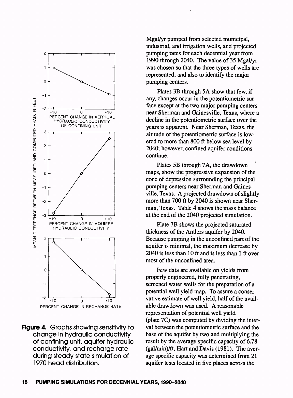
LU
X
Q
LU
I-
Q.
S
o
o
Q
LU
DC
CO
LU
DQ
LU
O
z
LU
cc.
LU
LL
LL
Q
-1
-2
-1
-2
-3
-10
0
+10
PERCENT
CHANGE
IN
VERTICAL
HYDRAULIC CONDUCTIVITY
OF
CONFINING
UNIT
-10
0
»10
PERCENT
CHANGE
IN
AQUIFER
HYDRAULIC
CONDUCTIVITY
-1
"
2
-10
0
+10
PERCENT
CHANGE
IN
RECHARGE
RATE
Figure
4.
Graphs showing
sensitivity
to
change
in
hydraulic
conductivity
of
confining
unit,
aquifer
hydraulic
conductivity, and
recharge
rate
during
steady-state
simulation
of
1970
head
distribution.
Mgal/yr
pumped
from
selected municipal,
industrial,
and
irrigation
wells,
and
projected
pumping
rates
for
each
decennial
year
from
1990
through
2040.
The
value
of
35
Mgal/yr
was
chosen
so
that
the
three
types
of
wells
are
represented,
and
also
to
identify
the
major
pumping
centers.
Plates
3B
through
5A
show
that
few,
if
any,
changes
occur
in
the
potentiometric
sur-
face
except
at
the
two
major
pumping
centers
near
Sherman
and
Gainesville,
Texas,
where
a
decline
in
the
potentiometric
surface
over
the
years
is
apparent.
Near
Sherman,
Texas,
the
altitude
of
the
potentiometric
surface
is
low-
ered
to
more
than
800
ft
below
sea
level
by
2040;
however,
confined
aquifer
conditions
continue.
Plates
5B
through
7A,
the
drawdown
maps,
show
the
progressive
expansion
of
the
cone
of
depression
surrounding
the
principal
pumping
centers
near
Sherman and
Gaines-
ville,
Texas.
A
projected
drawdown
of
slightly
more than
700
ft
by
2040
is
shown
near
Sher-
man,
Texas.
Table
4
shows
the
mass
balance
at
the
end
of
the
2040
projected
simulation.
Plate
7B
shows
the
projected
saturated
thickness
of
the
Antlers
aquifer
by
2040.
Because
pumping
in
the
unconfined
part
of
the
aquifer
is
minimal,
the
maximum
decrease
by
2040
is
less
than
10
ft
and
is
less
than
1
ft
over
most
of
the
unconfined
area.
Few
data
are
available
on
yields
from
properly
engineered,
fully
penetrating,
screened
water
wells
for
the
preparation
of
a
potential
well
yield
map.
To
assure
a
conser-
vative
estimate
of
well
yield,
half
of
the
avail-
able
drawdown
was
used.
A
reasonable
representation
of
potential
well
yield
(plate
7C)
was
computed
by
dividing
the inter-
val
between
the
potentiometric
surface
and
the
base
of
the
aquifer
by
two
and
multiplying
the
result
by
the
average
specific
capacity
of
6.78
(gal/min)/ft,
Hart
and
Davis
(1981).
The
aver-
age
specific
capacity
was
determined
from
21
aquifer
tests
located
in
five
places across
the
16
PUMPING
SIMULATIONS
FOR
DECENNIAL
YEARS,
1990-2040

Table
4.
Mass
balance
at
end
of
projected
simulation
to
2040
Cubic
feet
__________________per
second
Inflow:
Storage
20.42
Constant
head
81.94
Wells
0.00
Recharge
65.30
River
leakage
1.74
Head-dependent
boundary
1.37
Total
inflow
170.77
Outflow:
Storage
0.00035
Constant
head
28.40
Wells
69.07
Recharge
0.00
River
leakage
73.33
Head-dependent
boundary
0.00
Total
outflow
170.80
Inflow
-
Outflow
-0.028
study
area.
On
plate
7C
a
100-gal/min
contour
interval
shows
no
change
in
potential
well
yield
to
2040,
and
a
smaller
contour
interval
is
untenable.
Therefore,
drawdown
in
the
out-
crop
area
is
so
small
that
the
well
yields
are
expected
to
be
unchanged
during
the
simula-
tion
period.
In
the
confined
area,
well
yields
will
decrease
when
the
potentiometric
surface
falls
below
the
base
of
the
younger
confining
unit,
but
the
Antlers
aquifer
is so
thick that
well
yield
can
be
maintained
by
deeper
drill-
ing.
The
calculated
amount
of
water
in
storage
in
1970
was
916,556,000
acre-ft.
The volu-
metric
results
of
the
six
projections
are
shown
below.
The
rapid
decrease
in
storage
from
the
time
simulated
pumping began
(1970)
to
the
first
projection
year
(1990)
followed
by
a
marked slowing
of
the
rate
of
storage
decrease
is
typical
of
a
confined
aquifer.
Pumping
induces
vertical
leakage
through
the
confining
layer.
The
water
thus
transmitted
recharges
the
aquifer,
thereby
slowing
the
initial rate
of
stor-
age
loss
and
moderating
the
loss
through
time.
The
water
volumes
remaining
in
storage
for
1970
and
the
projection
years
are calcu-
lated
for
the
unconfined
part
of
the
modeled
area,
and
may
include
slightly
saline
water
in
the
southeast
part.
Because
of
the
elasticity
of
the
aquifer
and
the
very slight
compressibility
of
water,
a
small
additional
volume
of
water
would
be
recovered
from
the
confined
part
of
the
aquifer
as
water
levels
are
lowered
to
pro-
Projections
1990
2000
2010
2020
2030
2040
Water
pumped
since
1970
(acre-ft)
733,000
1,020,000
1,352,000
1,735,000
2,180,000
2,680,000
Water
remaining
in
storage
(acre-ft)
916,441,000
916,389,000
916,326,000
916,241,000
916,126,000
915,988,000
Decrease
in
storage
since
1970
(acre-ft)
115,000
167,000
230,000
315,000
430,000
568,000
Decrease
in
storage
since
1970
(percent)
0.012
0.018
0.025
0.034
0.047
0.062
PUMPING
SIMULATIONS
FOR
DECENNIAL
YEARS,
1990-2040
17
duce
unconfined
conditions.
Based
on
the rela-
tive
storage values
for unconfined
and
confined
conditions,
the
additional
volume
probably
is
less
than
0.3
percent.
If
the
poten-
tiometric
surface
in
the
confined
part
of
the
aquifer
declines
to
unconfined
conditions
as
the
result
of
increased
pumping,
not
all
the
water
in
storage
may
be
economically
recover-
able
because
of
increased lifting
costs,
espe-
cially
in
the
downdip
part
of
the
modeled
area.
SUMMARY
AND
CONCLUSIONS
The
Antlers
Sandstone
of
Early
Creta-
ceous
age
occurs
in
all
or
parts
of
Atoka,
Bryan,
Carter,
Choctaw,
Johnston,
Love,
Mar-
shall,
McCurtain,
and
Pushmataha
Counties,
a
4,400-square-mile
area
in
southeastern
Okla-
homa
parallel
to
the
Red
River.
The
sandstone
comprising
the
Antlers
aquifer
is
exposed
in
the northern
one-third
of
the
area,
and
ground
water
in
the
outcrop
area
is
unconfined.
Younger
Cretaceous
rocks
overlie
the
Antlers
in
the
southern
two-thirds
of
the study
area
where
the
aquifer
is
confined.
The Antlers
extends
in
the
subsurface
south
into
Texas
where
it
underlies
all
or
parts
of
Bowie,
Cooke, Fannin,
Grayson,
Lamar,
and Red
River
Counties.
An
area
of
approximately
5,400
square
miles
in
Texas
is
included
in
the
study.
The
Antlers Sandstone
consists
of
sand,
clay,
conglomerate,
and
limestone
deposited
on
an
erosional
surface
of
Paleozoic
rocks.
Saturated
thickness
in
the
Antlers ranges
from
0
feet
at
the
updip
limit
to
probably
more
than
2,000
feet,
25
to
30
miles
south
of
the
Red
River.
Simulated
recharge
to
the
Antlers
based
on
model
calibration
ranges
from
0.32
to
about
0.96
inch
per
year.
Base
flow
increases where
streams
cross
the
Antlers
outcrop,
indicating
that
the
aquifer
supplies
much
of
the
base
flow.
Pumpage
rates
for
1980
in
excess
of
35
million
gallons
per
year
per
grid
cell
for
public
supply,
irrigation,
and
industrial
uses
total
872
million
gallons
in
the
Oklahoma
part
of
the
Antlers
and
5,228
million
gallons
in
the
Texas
part
of
the
Antlers.
Ground-water
flow
in
the
Antlers
aquifer
was
simulated
using
one active
layer
in
a
three-dimensional
finite-difference
mathemati-
cal
model.
Simulated
aquifer
hydraulic
con-
ductivity
values
range
from
0.87
to
3.75
feet
per
day.
A
vertical
hydraulic
conductivity
of
1.5
x
10"
4
foot
per
day
was
specified
for
the
younger
confining
unit
in
the simulation.
An
average
storage
coefficient
of
0.0005
was
specified
for
the
confined
part
of
the
aquifer;
a
specific
yield
of
0.17
was
specified
for
the
unconfined
part.
Because
pumping
from
the
Antlers
is
min-
imal,
calibration
under transient
conditions
was
not
possible.
Consequently,
the
head
changes
resulting
from
projection
simulations
in
this
study
are
estimates
only.
Ground-water
hydrologic
data
described
in
the
report
indi-
cates
that
steady-state
conditions
exist
throughout
most
of
the
Antlers
aquifer.
This
interpretation
is
supported
by
the
results
of
the
model
simulations.
Volumetric
results
of
the
six
projection
simulations
from
the
years
1990
to
2040,
usually
at
steadily
increasing
pump-
ing
rates, indicate that
the
decrease
in
the
vol-
ume
of
ground
water
in
storage
due
to
pumping
approximately
9,700,000
acre-feet
from
1970
to
2040
is
less
than
0.1
percent.
Therefore,
if
future
pumping
rates
do
not
sig-
nificantly
exceed
the
pumping
rates
used
in
the
six
projections,
the
quantity
of
water
in
the
Antlers
aquifer
should
be
virtually
unchanged
except
near
the
outcrop
limits
where
saturated
thickness
becomes
very
thin.
SELECTED
REFERENCES
Davis,
L.V.,
1960,
Geology
and
ground-water
resources
of
southern
McCurtain
County,
Oklahoma:
Oklahoma
Geological
Survey
Bulletin
86,
108
p.
Davis,
R.E.,
and
Hart,
D.L.,
Jr.,
1978,
Hydro-
logic
data
for
the
Antlers
aquifer,
south-
18
SUMMARY
AND
CONCLUSIONS
eastern
Oklahoma:
U.S.
Geological
Survey
Open-File
Report
78-1038,
24
p.
Environmental
Health
Services
State
Water
Quality
Laboratory,
1979,
Public water
supplies
for
the
State
of
Oklahoma,
south-
east
district:
Oklahoma
City,
Oklahoma
State
Department
of
Health,
108
p.
Fay,
R.O.,
1974,
Unpublished
reconnaissance
mapping
(for
Oklahoma
Geological
Sur-
vey)
in
Hart,
D.L.,
Jr.,
1974,
and
Marcher,
M.V.,
and
Bergman,
D.L.,
1983.
Fenneman, N.M.,
and
Johnson,
D.W.,
1946,
Physical
divisions
of
the
United
States:
U.S.
Geological
Survey,
1
sheet,
scale
1:7,000,000.
Frederickson,
E.A.,
Redman,
R.H.,
and
Wes-
theimer,
J.M.,
1965,
Geology
and
petro-
leum
of
Love
County,
Oklahoma:
Oklahoma
Geological
Survey
Circular
63,
91
p.
Freeze,
R.A.,
and
Cherry,
J.A.,
1979,
Ground-
water:
Englewood
Cliffs,
N.J.,
Prentice-
Hall,
Inc.,
604
p.
Freeze
and
Nichols,
Inc.,
1980,
Water
usage
and
supply
in
the
Texas
areas
of
the
Red
River
chloride
control
study;
Checkpoint
I
report:
Tulsa, Okla.,
U.S.
Army
Corps
of
Engineers,
417
p.
Hart,
D.L.,
Jr.,
1974,
Reconnaissance
of
the
water
resources
of
the
Ardmore
and
Sher-
man
quadrangles,
southern
Oklahoma:
Oklahoma
Geological
Survey
Hydrologic
Atlas
HA-3,4
sheets,
scale
1:250,000.
Hart,
D.L.,
Jr.,
and
Davis,
R.E.,
1981,
Geohy-
drology
of
the
Antlers
aquifer
(Creta-
ceous),
southeastern
Oklahoma:
Oklahoma
Geological
Survey
Circular
81,
33
p.
Havens,
J.S.,
and
Bergman,
D.L.,
1976,
Ground-water
records
for
southeastern
Oklahoma,
Part
1 Records
of
wells and
springs:
U.S.
Geological
Survey
Open-
File Report
76-889,
59
p.
Huffman,
G.G.,
Alfonsi,
P.P.,
Dalton,
R.C.,
Duarte-Vivas,
Andres,
and
Jeffiries,
E.L.,
1975,
Geology
and
mineral
resources
of
Choctaw
County,
Oklahoma:
Oklahoma
Geological
Survey
Bulletin
120,
39
p.
Huffman,
G.G., Hart,
T.A.,
Olson,
L.J.,
Cur-
rier,
J.D.,
and
Ganser,
R.W,
1978,
Geol-
ogy
and
mineral
resources
of
Bryan
County,
Oklahoma:
Oklahoma
Geologi-
cal
Survey
Bulletin
126,
113
p.
Johnson,
A.I.,
1967,
Specific
yield Compila-
tion
of
specific
yields
for
various
materi-
als:
U.S.
Geological
Survey
Water-
Supply
Paper
1662-D,
74
p.
Laine,
L.L.,
1963,
Surface
water
of
Kiamichi
River
basin
in
southeastern
Oklahoma,
with
a
section on
Quality
of
water,
by
T.R.
Cummings:
U.S.
Geological
Survey
open-file
report,
39
p.
Marcher,
M.V.,
and
Bergman,
D.L.,
1983,
Reconnaissance
of
the
water
resources
of
the
McAlester
and
Texarkana Quadran-
gles,
southeastern
Oklahoma:
Oklahoma
Geological
Survey
Hydrologic
Atlas
HA-
9,
4
sheets,
scale
1:250,000.
McDonald,
M.G.,
and
Harbaugh,
A.W.,
1989,
A
modular
three-dimensional
finite-differ-
ence
ground-water
flow
model:
U.S.
Geological
Survey
Techniques
of
Water-Resources
Investigations,
Book
6,
Chapter
A
1,586
p.
Nordstrom,
PL.,
1982,
Occurrence,
availabil-
ity,
and
chemical
quality
of
ground
water
in
Cretaceous
aquifers
of
North
Central
Texas:
Texas
Department
of
Water
Resources
Report
269,
v.
1,
61
p.;
v.
2,
386
p.
Oklahoma
Water
Resources
Board,
1985,
as
amended,
Rules,
regulations,
and
modes
of
procedure:
Oklahoma
Water
Resources
Board
Publication
126,
118
p.
Pettyjohn,
WA.,
White, Hal,
and
Dunn,
Shari,
1983,
Water
atlas
of
Oklahoma:
Stillwater,
SELECTED
REFERENCES
19

Okla.,
University
Center
for
Water
Research,
Oklahoma
State
University,
72
p.
Solley,
W.B.,
Chase,
E.B.,
and
Mann,
W.B.,
IV,
1983,
Estimated
use
of
water
in
the
United
States
in
1980:
U.S.
Geological
Survey
Circular
1001,
56
p.
U.S.
Department
of
Agriculture,
1966,
Soil
survey
of
Love
County,
Oklahoma:
Soil
Conservation
Service,
94
p.
1974,
Soil survey
of
McCurtain
County,
Oklahoma:
Soil
Conservation
Service,
99
p.
1977,
Soil
survey
of
Johnston
County,
Oklahoma:
Soil
Conservation
Service,
57
p.
1978,
Soil
survey
of
Bryan
County,
Oklahoma:
Soil
Conservation
Service,
110
p.
1979a,
Soil
survey
of
Atoka
County,
Oklahoma:
Soil
Conservation
Service,
85
p.
1979b,
Soil
survey
of
Carter
County,
Oklahoma:
Soil
Conservation
Service,
67
p.
1979c,
Soil
survey
of
Choctaw
County,
Oklahoma:
Soil
Conservation
Service,
87
p.
1979d,
Soil
survey
of
Pushmataha
County,
Oklahoma:
Soil
Conservation
Service,
75
p.
1980,
Soil
survey
of
Marshall
County,
Oklahoma:
Soil
Conservation
Service,
59
p.
U.S.
Department
of
Commerce,
1973,
Cli-
matography
of
the
United
States
no.
81
(Oklahoma),
Monthly
normals
of
temper-
ature,
precipitation,
and
heating
and
cool-
ing
degree
days
1941-70:
Asheville,
N.C.,
National
Oceanic
and
Atmospheric
Administration,
Environmental
Data
Ser-
vice,
10
p.
U.S.
Geological
Survey,
1966-67,
Water-
resources
data
for
Oklahoma,
1965-66,
Part
1 Surface-water
records:
U.S.
Geological
Survey
Water-Data
Report
(published
annually).
1978,
Water-resources
data
for
Okla-
homa,
water
year
1977 volume
2:
U.S.
Geological
Survey
Water-Data
Reports
OK-77-2
(published
annually).
1980-81,
Water-resources
data
for
Oklahoma,
water
years
1979-80
vol-
ume
2:
U.S.
Geological
Survey
Water-
Data
Reports
OK-79-2
to
OK-80-2
(pub-
lished
annually).
Wayland,
J.R.,
and
Ham,
WE.,
1955,
General
and
economic
geology
of
the
Baum
Lime-
stone,
Ravia-Mannsville
area,
Okla-
homa:
Oklahoma
Geological
Survey
Circular
33,44
p.
GLOSSARY
OF
TECHNICAL
TERMS
Acre-foot.
The
volume
of
water
required
to
cover
one
acre
to
a
depth
of
one
foot;
equivalent
to
43,560
cubic
feet
or
325,851
U.S. gallons.
Aquifer.
A
formation,
group
of
formations,
or
part
of
a
formation
that
contains
suffi-
cient
saturated
permeable
material
to
yield
significant
quantities
of
water
to
wells
and
springs.
Base
flow.
Sustained
or
fair-weather
runoff
usually
composed
mostly
of
ground-water
discharge.
Comanchean.
North
American
provincial
series:
Lower
and Upper
Cretaceous
(above
Coahuilan,
below
Gulfian).
Confined
ground
water.
Ground
water
under
pressure
significantly
greater
than
atmo-
spheric, the
upper
limit
of
confined
ground
water
is
the
bottom
of
a
bed
of
dis-
tinctly
smaller
hydraulic
conductivity
than
that
of
the
material
in
which
the
confined
water
occurs.
20
GLOSSARY
OF
TECHNICAL
TERMS

Conglomerate.
A
coarse-grained,
clastic
sed-
imentary
rock
composed
of
rounded
to
subangular
fragments
larger
than
2
milli-
meters
in
diameter
set in
a
fine-grained
matrix
of
sand,
silt,
or
any
of
the
common
natural
cementing
materials.
Cretaceous. The
final
period
of
the
Mesozoic
Era
thought
to
have
covered
the
span
of
,
time
between
138
and
63
million
years
ago;
also,
the
corresponding
system
of
rocks.
Darcy's
law.
An
equation expressing laminar
flow
of
fluids
through
permeable
material
in
which
inertia
is
neglected.
In
the
case
of
water,
flow
can
be
expressed
as:
Q
=
KIA
in
which
Q
is
the
discharge,
/
is
the
hydraulic
gradient, A
is
the
cross-sectional
area
at
right
angles
to
flow,
and
K
is
a
con-
stant
whose
value
depends
on
the
kind
of
permeable
material
and
the
viscosity
of
the
water.
Evapotranspiration.
Loss
of
water
from
a
land
area
through
transpiration
by
plants
and
evaporation
from
the
soil.
Also
the
volume
of
water
lost
through
evapotrans-
piration.
Gaining
stream.
A
stream
or
reach
of
a
stream
whose
flow
is
being
increased
by
inflow
of
ground
water.
Gulfian.
North
American
provincial
series:
Upper
Cretaceous
(above
Comanchean,
below
Paleocene
of
Tertiary)
Gradient.
The
rate
of
increase
or
decrease
of
a
quantity;
the
slope
or
grade.
Head,
static.
The
height
above
a
standard
datum
of
the
surface
of
a
column
of
water
(or
other
liquid)
that
can
be
supported
by
the
static
pressure
at
a
given
point.
Homogeneity.
Synonymous
with
unifor-
mity.
A
material
is
homogeneous
if
its
hydrologic
properties
are
identical
every-
where.
Hydraulic
conductivity.
If
a
porous
medium
is
isotropic
and
the fluid
is
homogenous,
the
hydraulic
conductivity
of
the
medium
is
the
volume
of
water
at
the
existing
kine-
matic
viscosity
that
will
move
in
unit
time
under
a
unit
hydraulic
gradient
through
a
unit
area
measured
at
right
angles
to
the
direction
of
flow.
Isotropic.
A
medium
whose
physical
proper-
ties
are
the
same in
all
directions.
National
geodetic
vertical
datum
of
1929.
A
geodetic
datum
derived
from
a
general
adjustment
of
the
first-order
level
nets
of
both
the
United
States
and
Canada,
for-
merly
called
Mean
Sea
Level.
Paleozoic.
An
era
of
geologic
time,
from
the
end
of
the
Precambrian
to
the
beginning
of
the
Mesozoic,
from
about
570
to
about
240
million
years
ago.
Pennsylvanian.
A
period
of
the
Paleozoic
Era,
and
its
corresponding
system
of
rocks,
thought
to
have
covered
the
span
of
time
between
330
and
290
million
years
ago.
Permian.
The
last
period
of
the
Paleozoic
Era,
and
its
corresponding
system
of
rocks,
thought
to
have
covered
the
span
of
time
between
290
and
240
million
years
ago.
Potentiometric
surface.
A
surface
that repre-
sents
the
static
head.
As
related
to
an
aquifer,
the
potentiometric
surface
is
defined
by
the
levels
to
which
water
will
rise
in
tightly
cased
wells.
The water
table
is
a
particular
potentiometric
surface.
Recharge.
The
process
involved
in
the
absorption
and
addition
of
water
to
the
zone
of
saturation.
Also,
the
amount
of
water
added.
Return
flow.
Irrigation
water
not
consumed
by
evapotranspiration
but
returned
to
its
source
or
to
another
body
of
ground
or
surface
water.
GLOSSARY
OF
TECHNICAL
TERMS
21
Saturated
thickness.
The thickness
of
the
zone
below
the
water
table
in
which
all
interstices
are
filled
with ground
water.
Specific
yield.
The
ratio
of
(1)
the
volume
of
water
that
the
rock
or
soil,
after
being
sat-
urated,
will yield
by
gravity
to
(2)
the
vol-
ume
of
the
rock
or
soil.
The
definition
implies
that gravity
drainage
is
complete.
Steady-state. In
steady-state
flow,
as
of
ground
water
through
a
permeable
mate-
rial,
there
is
no
change
in
head
with
time.
Storage
coefficient.
The
volume
of
water
an
aquifer releases
from
or
takes
into
storage
per
unit
surface area
of
the
aquifer
per
unit
change
in
head.
Stratigraphy.
The
branch
of
geology
that
deals
with
the
definition
and
description
of
major
and
minor
natural
divisions
of
rocks
in
outcrop
or
from
the
subsurface,
and
with the
interpretation
of
the
signifi-
cance
of
such
divisions.
Transgressive.
Sediments
deposited
during
the
advance
or
encroachment
of
water
over
a
land
area
or
during
the
subsidence
of
the
land,
and
characterized
by
an
onlap
arrangement.
Transient
simulation.
A
model
simulation
in
which
heads
in
the
aquifer
and
in
the
con-
fining
beds,
in
the
case
of
a
confined
aqui-
fer with
leakey
confining beds, vary with
time.
Transmissivity.
The
rate
at
which
water
of
the
prevailing
kinematic viscosity
is
trans-
mitted
through
a
unit
width
of
the
aquifer
under
a
unit
hydraulic
gradient.
Unconfined
water.
Ground
water
in
an
aqui-
fer
that
has
a
water
table.
Water
table.
The
water
surface
in
an
uncon-
fined
water
body
at
which
the
pressure
is
atmospheric.
The
water
table
is
defined
by
levels at
which
water
stands
in
wells
that
penetrate
the
water
body
just
far
enough
to
hold
standing
water.
In wells
that
penetrate
to
greater
depths,
the
water
level
will
stand above
or
below
the
water
table
if
an
upward
or
downward
compo-
nent
of
ground-water
flow
exists.
22
GLOSSARY
OF
TECHNICAL TERMS
*U.S.
GOVERNMENT
PRINTING
OFFICE:1992-769-117
