ISSN: 1962-5361
Disclaimer: This Philadelphia Fed working paper represents preliminary research that is being circulated for discussion purposes. The views
expressed in these papers are solely those of the authors and do not necessarily reflect the views of the Federal Reserve Bank of
Philadelphia or the Federal Reserve System. Any errors or omissions are the responsibility of the authors. Philadelphia Fed working papers
are free to download at: https://philadelphiafed.org/research-and-data/publications/working-papers.
Working Papers
Assessment Frequency and Equity
of the Real Property Tax: Latest
Evidence from Philadelphia
Yilin Hou
Maxwell School, Syracuse University
Lei Ding
Federal Reserve Bank of Philadelphia Community Development and Regional Outreach
David J. Schwegman
School of Public Affairs, American University
Alaina G. Barca
Federal Reserve Bank of Philadelphia Community Development and Regional Outreach
WP 21-43
December 2021
https://doi.org/10.21799/frbp.wp.2021.43
COMMUNITY DEVELOPMENT AND REGIONAL OUTREACH

Assessment Frequency and Equity of the Real Property Tax:
Latest Evidence from Philadelphia
Yilin Hou, Lei Ding,* David J. Schwegman, Alaina G. Barca
December 2021
Hou: Maxwell School, Syracuse University
Ding and Barca: Federal Reserve Bank of Philadelphia
Schwegman: School of Public Affairs, American University
* Contact author: lei.ding@phil.frb.org. The authors thank Jeffrey Lin, Keith Wardrip, and Stephen Ross for
their helpful comments. The views expressed in these papers are solely those of the authors and do not
necessarily reflect the views of the Federal Reserve Bank of Philadelphia or the Federal Reserve System. Any
errors or omissions are the responsibility of the authors.

1
Abstract
Philadelphia’s Actual Value Initiative, adopted in 2013, creates a unique opportunity for
us to test whether reassessments at short intervals to true market value and taxing by such values
improve equity. Based on a difference-in-differences framework using parcel-level data matched
with transactions in Philadelphia and 15 comparable cities, this study finds positive evidence on
equity outcomes from more regular revaluations. The quality of assessment, as measured by the
coefficient of dispersion, improves substantially after 2014, although the extent of improvement
varies across communities. Vertical equity, measured by price-related differential, also
improved, although it was still above the standard threshold. Cross-city comparisons confirm
Philadelphia’s improvement in quality and equity of assessments after adopting the initiative.
These results highlight the importance of regular reassessment in places where property values
increase quickly, and they shed light on the disparate impacts of reassessment across income,
property value, race, and gentrification status. The paper makes the case that the property tax, if
designed well, can be an equitable tax instrument.
Key words: real property tax; valuation; assessment cycle; equity
JEL codes: H20, H31, H71, R51

2
1. Introduction
Although the property tax has long been criticized as the most unfair, even “the worst”
tax (Jensen, 1931; Fisher, 1996; Cabral and Hoxby, 2012), it has persisted through today in the
United States as the most important own-source revenue for many local governments. It is fair to
say that local autonomy thrives when localities control their own mainstay revenue. For this
important reason, improving the administration of the property tax is a perennial task for the
public finance community. The negative reputation of the property tax is derived mainly from
issues and challenges in property valuation, which demands up-to-date information about
multiple aspects of properties and requires trained professional staff, thereby posing high costs in
terms of technology and personnel. On top of these difficulties, property valuation is also
susceptible to idiosyncratic errors in assessment. Property assessment, thus, is a complex,
constantly evolving field.
Lags in property reassessment — or delays in estimating changes in the value of a
property since the last assessment — and poor tax collection can adversely affect the horizontal
and vertical equity of any local property tax system, as well as erode a local government’s
revenue-raising capacity (Weber et al., 2010). Sudden and unexpected changes in tax bills from
inaccurate assessments can leave capital-wealthy but liquidity-constrained households unable to
pay their tax bills (Alm et al., 2016). Furthermore, the property tax is sometimes referred to as
the “least fair” tax by the average American (ACIR, 1987; Fisher, 1996; Cabral and Hoxby,
2012): Property taxes are often found to be regressive, such that lower-value properties face
higher assessments relative to their actual market values than higher-value properties (Berry et
al., 2021; McMillen, 2013; McMillen and Singh, 2020). In particular, in jurisdictions where
regular reassessment is not mandated by the state, fairness in taxation becomes a serious concern,

3
as house appreciation is less likely to be included in the assessed value owing to long lags in
reassessment.
This study evaluates whether reassessments at short intervals to true market value and
taxing by such values improve equity. In most states, real property tax law requires regular
revaluation of properties. For example, counties in the state of Washington are required to
annually update assessed values of all properties based on appropriate statistical data, and they
are also required to physically inspect properties at least once every six years.
1
The state of
Pennsylvania, however, is one of the few states that does not have statutorily mandated
reassessments on a fixed cycle (Montarti and Weaver, 2007). In Philadelphia,
2
historical lags in
property assessment have resulted in systematic inequities in the city’s property tax system.
From the 1980s to 2012, Philadelphia did not conduct a comprehensive reassessment. As a
result, the assessed value listed on most property tax bills was estimated to be 60 percent lower
than true market values (Dowdall and Warner, 2012; Ding and Hwang, 2020). The quality of
assessments was poor, and properties with similar market values were often listed with
dramatically different assessed values (Gillen, 2008). As assessments were increasingly out of
line with actual property values and the tax burden had become increasingly unequal with respect
to wealth, Philadelphia adopted a property tax reform in 2013, known as the Actual Value
Initiative (AVI). The AVI was not only the first comprehensive revaluation of all properties in
the city in a 30-year window but also broke from the tradition of fractional assessment to
reassess all properties at full market value. To improve the quality of property assessments,
under the AVI, the city reassessed every property and changed in 2014 how tax bills were
calculated. Philadelphia conducted another comprehensive revaluation in 2019.
1
See dor.wa.gov/sites/default/files/legacy/docs/pubs/prop_tax/homeown.pdf.
2
Throughout this paper, Philadelphia refers to the city of Philadelphia, rather than the metropolitan area.
4
The AVI requires more regular revaluations to address issues related to poor assessment
quality and increasing inequity in property taxation in Philadelphia. As a policy shock, it
provides a unique opportunity for us to answer our research question: Do regular short cycles of
reassessment generate an equitable distribution of the tax burden among property owners? The
consensus among scholars and practitioners is that annual reassessment best maintains equity and
efficiency (Dowdall and Warner, 2012; Weber et al., 2010). Given the high costs of annual
reassessments, however, a vast majority of assessing jurisdictions nationwide conduct
reassessments less frequently. This overarching question in fact embeds several minor but not
less important subquestions: What is the impact of regular comprehensive reassessments on
properties across neighborhoods? Are more regular reassessments alone sufficient to achieve the
equity goal? And if not, what other assessment practices could improve equity in property
taxation? With empirical estimates on horizontal and vertical equity, we then consider the
ramifications of assessment cycles on the efficiency of the cycles in terms of possible behavioral
patterns of property owners.
Taking Philadelphia’s two recent reassessments as natural experiments, this paper uses
parcel-level data matched with sales transactions in Philadelphia and 15 comparable cities across
the nation to examine whether regular reassessments at short intervals to true market value and
taxing by such values improve horizontal and vertical equity. Horizontal equity, measured by the
coefficient of dispersion (COD) in this paper, measures the level of assessment uniformity:
whether parcels with the same (or close) attributes would be assessed and taxed at equal
amounts. Vertical equity, measured by the price-related differential (PRD), is concerned with the
inequality in assessments for properties of varying values: whether less expensive properties are
systematically assessed at higher ratios relative to their market values and thus bear a higher than
5
the fair share of property taxes than more expensive properties. The results suggest that before
the AVI, the quality of Philadelphia’s property assessments was worse than almost all other
cities in our sample and property taxes in Philadelphia were much more regressive than other
cities, as well. Pursuant to the AVI, the comprehensive revaluation in 2014 (and again in 2019)
led to marked improvement in assessment quality (horizonal equity), although the extent of
improvement in uniformity was much smaller in disadvantaged communities.
The vertical equity of Philadelphia’s property tax system also improved after the city
adopted the AVI. While a PRD between 0.98 and 1.03 is generally considered as the acceptable
range, Philadelphia had a PRD as high as 1.42 pre-AVI, suggesting lower‐priced homes were
systematically assessed at a greater percent of their market values than high-value ones. The
PRD declined to 1.28 in 2014 and further to 1.14 in 2019, showing a continued mitigation of
assessment inequity post-AVI. Effective tax rates also experienced larger declines for properties
in more disadvantaged communities, namely majority-Black or high-minority neighborhoods,
low-income neighborhoods, or lower-income nongentrifying neighborhoods. Cross-city
comparisons confirm that assessment quality in Philadelphia improved substantively against
other cities after 2014, although Philadelphia’s PRD remained above the popular threshold.
Overall, our results highlight the importance of regular reassessments in cities that
experienced large increases in property values (e.g., through gentrification) and shed light on the
disparate impacts reassessment might have across income, property value, race, and
gentrification. Thus, the paper makes the case that with regular reassessments, the real property
tax can be an effective tax instrument, with facilitation by other practices or tax relief programs
to ensure and maintain an equitable impact. This paper contributes to the literature on property
taxation in a number of ways. First, the policy shock of the AVI allows us to identify the causal
6
effects of more regular reassessments on improving assessment quality and redistributing the
property tax burden. This paper provides updated evidence on the (horizontal and vertical) equity
effects of property revaluation after a long lapse in reassessments. Second, this study looks into
the heterogeneity of the effects among properties in different neighborhoods and find that more
regular reassessments provide greater benefit for property owners in more disadvantaged
neighborhoods, although assessment accuracy does not necessarily improve as much. Finally,
our research question cuts deep to the core of property tax administration — equity and
efficiency. Conventional taxation theory has these two principles as holding a tradeoff. We argue
that in terms of the property tax, equity and efficiency can move in unison — raising one will not
lower the other, but rather the two will mutually reinforce through more frequent, regular
property tax reassessments.
2. Analytical Framework and Context
2.1. Property Assessment and Rationales
Value Assessment
Value assessment in property taxation determines the tax base of each property at some
snap point of time via obtaining an as accurate as possible estimate of the market value of a
property. Estimates are then converted into assessments either at 100 percent of market value or
at a uniform percentage (assessment ratio) of the market value. The former is full value
assessment, whereas the latter is a fractional assessment. As long as the estimates are accurate,
the assessed value, A, matches the market value, V, providing a reliable tax base.
The purpose of obtaining accurate estimates of market value is to equitably distribute the
burden of financing local public services, with the assessed value as a ratio of the total tax base.
7
The rationale for regular reassessment is that market value fluctuates. Although the value of
properties trends up over time, the extent of change can be very uneven across neighborhoods,
property types, and value ranges in a jurisdiction. It is a heterogeneous process on several
dimensions. At the neighborhood level, amenities and typological features are one dimension. By
housing type, some appreciate quickly, some slowly, and some do not grow or even depreciate.
Along the range of housing prices (quality), the elasticity of demand and supply is another
dimension to consider.
The property tax is a levy on the stock of household wealth. The heterogeneity of value
changes over time demands regular reassessments to distribute the burden of public services on
the basis of household wealth. Absent regular assessments, the distribution of the tax burden
among properties will not be equitable, eroding the fairness of the tax and trust of the public in
government.
Assessment Cycles
In this paper, we use the following working definitions of assessment cycles and this
paper explores the relationship between the length of assessment cycles and a set of equity
(uniformity) measures. Comprehensive assessment (mass appraisal) is conducted in discrete
cycles by the year (valuation upon transaction or upon completion of new construction is
different). The shortest cycle is annual, which offers the highest probability of match between
market value (V) and assessed value (A), , which is the best for securing equity; thus, it is
the ideal cycle. The annual cycle is taken as the default. There can be a parameter before A,
, 0 < 1. When a jurisdiction uses estimated market value as assessed value, = 1;
when a jurisdiction uses a fractional assessment system, < 1.
8
We classify time between reassessments by three categories. The first category, a short
cycle, refers to one that reassesses every two or three years. Short cycles are suboptimal relative
to annual valuations, but the annual cycle is often not practicable for various reasons. For
example, a small jurisdiction or one with inadequate resources cannot afford to assess each year.
Uniformity of assessment from each comprehensive assessment can maintain most of its force
within a reasonably short period; thus, a short cycle may maintain uniformity before a large
inequity occurs. Short cycles arise as a compromise from the ideal cycle, often as the result of
balancing the high cost of an annual cycle with uniformity of valuation.
The second category, a regular cycle, refers to assessments that are conducted once every
four to six years. Although longer than a short cycle, these cycles are at least regular. The
regularity of valuation between two assessments mitigates erosion to uniformity (equity) to a
limited extent. These cycles often are adopted by small taxing jurisdictions, mainly for cost
reasons.
Finally, a long or irregular cycle refers to assessment cycles that are longer than six
years, beyond the length of a full economic cycle. These long cycles often become or drag into
irregular, indefinitely long cycles. These are the scenarios that have often occurred, caused
extreme inequity, and triggered the tag of the “worst tax.”
Under the U.S. federal system, states fall in at least two types — strong states and home
rule states — in their relation with localities in the regulation of local taxation. The former type
are Dillon-rule states that not only stipulate short or regular cycles but also strictly enforce the
required cycle. Take Virginia, for example: the 1984 revision of the Virginia Code requires
counties and cities to adopt a regular (fixed-length) cycle. The latter type allows local discretion,
9
without stipulating much regulation. New York is an example of home rule states, where local
taxing jurisdictions decide their own assessment cycles.
The administration of the property tax has evolved toward regular, short, preferably
annual reassessments, which are also what the states have mostly tried to promote since the
second half of the 20th century. Among the rationales for the preferred cycles is a technical
consideration: assessment is heavily subject to human judgment based on limited information,
out of which errors are unavoidable. The technical errors capitalize into property values and, if
not corrected in a timely manner, can erode tax equity for years.
2.2 Gaps in What Is Known
The academic literature has been thin on the administration of the property tax in general
and on the effects of assessment cycles in particular. Among the few earliest studies, Geraci
(1977) and Bowman and Mikesell (1990) identified some determinants of assessment equity,
including characteristics of assessors, staffing of the assessor’s office, and tools for valuation.
Mikesell (1980) examined the impact of assessment cycles on assessment quality. Using data
from Virginia local tax assessing units in the years 1973 through 1976, he found that 68 percent
of the units in regular cycles had better outcomes (higher uniformity or a 10 percent lower COD)
compared with units in annual reassessment, and he found much smaller improvement in the
latter group. He speculated that in states that require annual reassessments, revaluations were
often just copying prior years’ numbers, probably with a flat percentage adjustment for all
properties.
More recent research better accounts for potential simultaneity and omitted variable bias.
Using cross-sectional data (1992) of assessing towns and cities in New York, Eom (2008) found
10
a positive relationship between assessment uniformity and frequent reassessment. Specifically,
each additional year of lag in reassessment may lead to a 1.6 percent reduction in assessment
uniformity, while an additional reassessment over the previous four years improves uniformity
by 17.8 percent. However, there has not been more recent updated empirical evidence to support
that annual reassessment should be the norm or that short and regular cycles are preferred. This
paper fills the niche.
2.3 The Actual Value Initiative of Philadelphia
In 2013, after several years of public discussions and evaluations, Philadelphia adopted a
comprehensive property tax reform, known as the Actual Value Initiative (AVI), which became
effective for property tax bills in 2014. Under the AVI, Philadelphia conducted the first
comprehensive reassessment since the 1980s for the market value of every property in the city.
Consequently, the newly assessed values of properties under the AVI would more accurately
reflect their market values. For example, from 2005 to 2013, the mean assessed value of single-
family residential properties in Philadelphia remained almost flat, but after the full market value
reassessment, the average assessed value almost tripled (Ding and Hwang, 2020). All properties
were reassessed again at full market value in 2019.
Under the AVI, the city also changed the way it calculates tax bills (Ding and Hwang,
2020; Dowdall, 2015). Specifically, before 2013, the city used fractional assessment, at 32
percent (a predetermined ratio), so that less than one-third of a property’s estimated market value
counted as assessed value, and the nominal tax rate was 9.771 percent. The AVI replaced
fractional assessment with full market value assessment, with 100 percent of a property’s
estimated value as assessed value to calculate tax bills. Claimed to be a revenue-neutral reform,
11
the AVI redistributed the tax burden in the city, and the nominal tax rate plummeted to 1.34
percent in 2014. Properties with no or small increases in market values since the 1980s benefited
with lowered tax bills, whereas those with large appreciations in value received larger tax bills.
The effects of the two reassessments under the AVI are very clearly illustrated in Figure
1, where the dashed line marks the mean assessed values and the solid line marks the mean
market values for single-family residential homes. Between tax years 2010 and 2013, there was
very little change in the average assessed value for these properties; only new sales or properties
under appeals were likely to be reassessed. Beginning in 2014, an almost three-fold increase in
the assessed value considerably closed the difference between the average assessed value and the
average market value. Absent comprehensive reassessments from 2014 through 2018 (there was
a small increase in the tax rate in 2016 from 1.34 percent to 1.4 percent), the gap grew wider
again, with assessed value decreasing slowly, likely because of appeals and market value
increasing quickly. Then the second comprehensive full value reassessment in tax year 2019
closed some of the gap between the two values. Overall, the recent AVI tax reform in
Philadelphia as a natural experiment offers the best and most representative case for our study.
While the AVI requires the city to reassess all properties more regularly, it does not
necessarily change the administration of property assessment practices or the quality of
assessments. In other words, while a comprehensive reassessment should render the assessed
values closer to true market value, it does not necessarily make assessments more equitable, and
its effectiveness is still an empirical question.

12
3. Data and Methodology
3.1 Methodology
This study intends to isolate the effect of the AVI on the level of horizontal and vertical
equity of residential property assessments by comparing the assessment outcomes before and
after the adoption of the AVI in Philadelphia with those of a national sample of peer cities. Here,
properties (sales) in Philadelphia are considered as the treatment group because they became
subject to regular revaluation under the AVI post-2014. Properties in peer cities that did not
experience such a policy shock are considered as the comparison group. The two-way, property-
level, difference-in-differences (DID) model can be specified as:
Y
ijt
= β
0
+ β
1
TREAT
j
+ β
2
POST
t
+ β
3
TREAT
j
*POST
t
+ ΘTRACT
j
+ λYEAR
t
+ ε
ijt
(1)
in which Y
ijt
represents the outcome measure for property i in tract j and in year t. TREAT
j
is the
dummy variable that represents properties in Philadelphia (the treatment group). POST
t
is the
time dummy and is assigned a value of one for the post-2014 period. TREAT
j
*POST
t
is the two-
way interaction of the treatment and the time dummies. While both TREAT
j
and POST
t
are
omitted in the estimation because we include the tract and yearly fixed effects in our model, we
can still identify the effects of AVI by estimating the coefficient, β
3
, of the interaction term,
TREAT
j
*POST
t
. TRACT
j
and YEAR
t
are vectors of tract- and year-fixed effects.
To evaluate the heterogeneity in the effects of the AVI across neighborhoods that differ
by income, racial composition, and gentrification status (for the definition in this paper, see
footnote 15), we employ the following model using data from Philadelphia only.
Y
ijt
= β
0
+ β
1
NBHD
j
+ β
2
POST
t
+ β
3
NBHD
j
*POST
t
+ ΘTRACT
i
+ λYEAR
t
+ ε
ijt
(2)

13
in which NBHD represents the different types of neighborhoods (by race, income, or
gentrification status) and the coefficient of the interaction, β
3
, captures the change in the outcome
measures post-AVI in the corresponding type of neighborhoods relative to the change in the
reference group. In other words, β
3
measures how the AVI impacts properties in a particular type
of neighborhood differently from other neighborhoods. All other terms are as defined in equation
(1) above.
3.2 Measures of Horizontal and Vertical Equity
Horizontal equity (i.e., assessment uniformity) is concerned with assessment
differentiation between parcels with the same (or close) attributes. Thus, a uniform assessment,
with all properties of equal value being assessed and taxed at equal amounts, achieves horizontal
equity. Vertical equity is concerned with the treatment of properties over the range of values.
Applying different assessment ratios to properties of varying values results in vertical inequity.
For example, a system in which less expensive homes are systematically assessed at higher sales
ratios than more expensive homes is regressive, while a system in which the assessment ratio
increases as property value increases is progressive. When the ratio is consistent across home
values, a property tax system is considered equitable.
The assessment ratio (R) is defined as the assessed value of a property to the actual sale
price of the property (assessed value [A
i
] divided by market value [V
i
] in the year the property is
sold): = /, in which V
i
can be proxied by the recorded sales price of each property. This
measure could capture both horizontal and vertical equity, with the major limitation that it does
not directly measure any deviation from the desired threshold.

14
The International Association of Assessing Officers (IAAO) has suggested acceptable
thresholds as industry standards for horizontal equity and vertical equity in property assessment.
Here, we discuss two measures, coefficient of dispersion (COD) for horizontal equity and price-
related differential (PRD) for vertical equity, that are most often used in the literature. Taken
together, the COD and the PRD characterize the degree of assessment equity in a particular
housing market.
Measure of Horizontal Equity
The most common measure to assess horizontal equity is the COD, which measures the
average percent deviation of an individual parcel i's assessment ratio from the target (or median)
assessment ratio in a jurisdiction. The calculation of the COD of a sample of sales transactions
can be expressed as:
=
|
|
= |1
| (3)
where R
0
is the target assessment ratio in the taxing jurisdiction. In an ideal scenario, every
property would be assessed exactly at its market value, and thus each property would have an R
i
of “1.” So we use a value of “1” for R
0
, and then the mean COD is computed as the average
COD across all properties. Higher values of COD indicate less uniformity in assessment, while
lower COD values suggest relatively uniform assessments, and thus imply that a property tax
system is horizontally equitable.
According to the IAAO Standard on Ratio Study (2013), a reasonable COD for single-
family homes is between 5 percent and 15 percent, conditional on the age of the property and
neighborhood type, and the target COD for residential properties in “older, heterogeneous areas”

15
such as Philadelphia should be 15 percent or less.
3
Accordingly, we also created a dummy
variable that equals 1 if a sale has a COD of 15 percent or less.
To measure the actual tax burden for property owners, we use the effective tax rate as
another outcome, which is calculated as the tax amount divided by the market value of the
property proxied by sales price of arm’s length transactions.
Measure of Vertical Equity
While there is a general consensus that the COD is an appropriate measure to examine
horizontal equity, there is no such consensus over how to test the vertical equity of a property tax
system. We use the PRD as the primary measure of vertical equity,
4
which is calculated by
taking the mean assessment ratio for all parcels in the sample and dividing it by the weighted
mean ratio, where the weight is the sale price. This calculation can be expressed as:
=
[4]
A PRD of 1 thus implies an absence of vertical inequity in property assessment in a
particular geography: Assessments would be perfectly uniform across home values if the
weighted mean is equal to the unweighted mean. A PRD greater than 1 suggests the presence of
assessment regressivity, in which higher-value properties are assessed at lower ratios, and higher
3
As Eom (2008) notes, there is a nonlinearity inherent in the COD — it is much easier to decrease a COD from 30
percent to 20 percent than from 15 percent to 5 percent.
4
There are some important limitations with the PRD in measuring vertical equity, because PRD tends to be
estimated downward because of right-lying outliers that skew the distribution (Almy et al., 1978; Gloudemans,
1999; Carter, 2016). A number of strategies to evaluate the vertical equity of a tax system have been proposed (see
Paglin and Fogarty, 1972; Cheng, 1974; Almy et al., 1978; Bell,1984; Sunderman et al., 1990; and Kochin and
Parks, 1982).

16
values of PRD indicate greater regressivity. A PRD less than 1 instead suggests the presence of
assessment progressivity, in which lower-value properties are assessed at lower ratios.
The IAAO Standards (2013) suggest a PRD between 0.98 and 1.03 as the acceptable
range. This range is asymmetric around 1 because there is an upward bias in the denominator,
which does not affect the numerator. A PRD above 1.03 is generally considered regressive, i.e.,
favoring high‐valued homes, while a PRD below 0.98 is deemed progressive, which favors low‐
valued homes.
3.3 Data
Data used in this study primarily are obtained from two sources, in addition to data from
the U.S. Census Bureau (the 2009–2013 American Community Survey and U.S. Census
TIGER/Line Shapefiles). The first source is the publicly available administrative parcel-level
data from the City of Philadelphia’s Department of Revenue (DOR), the Philadelphia
Department of Records, and the Office of Property Assessment (OPA). The parcel-level tax files
contain annual assessed values, characteristics of each parcel (e.g., property type: residential or
commercial, single-family, condo, or multifamily), tax amount, as well as exemptions and
abatements, all from 2010 to 2019. Each parcel has a unique identifier that enables us to match
units across data sets. We also used real estate transfer data compiled by the Philadelphia
Department of Records,
5
which were merged to respective parcels; thereby, we have information
on assessments and taxes for properties that were transferred during the study period. Using
ArcGIS, we also conducted a spatial join to link property-level data to Philadelphia’s census
tracts.
5
These are available through OpenDataPhilly at www.opendataphilly.org/.

17
The administrative data from Philadelphia are compared with control group data from
CoreLogic Solutions, the latter of which were used to construct a transaction and assessment data
set for our control group of comparable cities for the 2012–2015 period.
6
The selection criteria
are: (1) the 30 largest U.S. cities and one smaller peer city, Pittsburgh, from Pennsylvania based
on its similarities to Philadelphia; (2) cities with consistent and reasonable counts of observations
in the data set during our sample period; (3) cities that conducted no comprehensive overhaul of
their assessment system based on our knowledge during our sample period. Applying these
criteria, we narrowed down to 15 cities. They are Baltimore; Charlotte, NC; Columbus, OH;
Dallas; Denver; El Paso, TX; Fort Worth, TX; Houston; Oklahoma City; Phoenix; Pittsburgh;
Portland, OR; San Antonio; Seattle; and Washington, D.C. A few other major cities, such as
New York, Chicago, and Los Angeles, were not selected, primarily because of either limited
coverage during the study period or a significant number of observations with missing values in
their assessment or sales data.
We made a few additional decisions in creating the final sample of residential properties
for our analysis.
7
First, the analysis focuses only on arm’s length transactions of single-family
residential properties. Arm’s length transactions generally refer to market-rate sales involving
buyers and sellers with no previous relationship (rather than, for example, sales between relatives
or foreclosure auctions). Prices from arm’s length transactions thus should better reflect true
market values, since buyers and sellers in these transactions are more likely to be seeking a price
that maximizes their own self‐interest. We focused on single-family home sales primarily
because of the higher volume of sales within this property class compared with other types of
6
Unfortunately, CoreLogic Solutions only offered this data set to us through 2015.
7
In addition to the two decisions discussed in the text, we also limited each property parcel to one transaction per
month to remove duplicates. If there were multiple transactions of the same property parcel in a month, we only
included the transaction with the highest price.

18
residential units, such as multifamily residential and condo units. Additionally, single-family
homes have a higher within-class uniformity than other property classes.
Second, sales with a missing value for the sales price, extremely low or high prices (those
with assessed values below $1,000 or above $2,000,000), or with extremely high or extremely
low assessment ratios were excluded from the analysis. The sales prices for 4.8 percent of sales
are missing in Philadelphia; another 26.9 percent of sales have sales prices below $1,000.
8
These
observations were excluded to mitigate the bias induced by these outliers. In addition, a small
share of sales transactions suffer from the issue of invalid transactions, as a 2018 audit report of
the Philadelphia OPA highlighted, for which we can conclude quite confidently that either the
sale price is not valid, the assessment does not reflect current market conditions, or the property
data underlying the assessment is far from accurate.
9
Because it is impossible to verify the
validity for millions of sales over multiple years, we followed the IAAO-recommended
maximum trimming limits
10
and excluded sales with assessment ratios above 3.0 or below 0.1
(about 5 percent on each side), which represent a further 9.1 percent of transactions.
11
After
trimming, the statistics provide a more logical and meaningful basis to come to informed policy
recommendations and tax administration practices.
8
Sales prices were recorded as $1 in 20.1 percent of sales, meaning these were not arm’s length sales. Our trends
were robust to alternative exclusion thresholds.
9
By the 2018 audit report of Philadelphia OPA: “Some, if not many, of the sales as identified as valid by the City are
not truly valid. This makes it impossible to continue the analysis without considering further action to yield a
clearer insight regarding assessment accuracy.”
10
The IAAO Standard states it is appropriate to set maximum trimming limits of no more than 10 percent (20
percent in extreme circumstances with small samples). We use an acceptable level of trimming — about 10 percent
of observations — to drop the outliers, while making sure the final sample still allows for a meaningful analysis and
reflects actual overall performance.
11
And the share of sales with invalid or small sales prices or with particularly large or small assessment ratios
decreases slightly over time during the study period. Thus, our results are likely an underestimate of the AVI’s
impact.
19
These data cleaning procedures were followed also for the control cities. The data are
made up of single-family properties, with duplicate month-property records cleaned; extreme
sales prices were removed; the same boundaries of assessment ratio values were trimmed; and
sparse tracts were removed. We also removed cities with sparse or inconsistent amounts of data
across years and focused on the years 2012–2015 in order to retain the 15 selected cities.
Our final sample has 156,171 sales transactions during the 2010 to 2019 period in
Philadelphia for our baseline regression. For the cross-city regression, there are 704,899
observations for the control group and 54,683 for the treatment (Philadelphia) of single-family
home transactions during the 2012–2015 period.
4. Impact of AVI on Equity: Descriptive Analyses
4.1 Horizontal Equity
Table 1 provides summary statistics of single-family residential properties in Philadelphia
by year from 2010 to 2019, where columns (1) to (4) are contextual information and columns (5)
to (9) are analytical indexes derived from the first four. The number of transactions and mean
sale price were both low through 2012 as part of the sluggish recovery from the Great Recession.
The market began to warm up in 2013 and has been improving since, with transactions and sale
prices smoothly trending up. From 2010 through 2013, the mean assessment ratio stayed in the
mid-50s, with the CODs also in the mid-to-high-50s, almost four times the acceptable level of 15
percent set by the IAAO for “old, heterogeneous areas” like Philadelphia. The percentage of
CODs below 15 percent was in the single digits, and the PRD was way above the IAAO
threshold.

20
Adopted as a response to increasing inequity in property taxation, the AVI seemed to
have done what it is supposed to do. The average assessment ratio more than doubled, increasing
to 119 percent in 2014. That is, the AVI led to increased assessed values in general, and an
average greater than 100 percent suggests that at least a significant share of assessments were
higher than their actual sale prices. The average COD decreased by a quarter from 55 percent in
2013 to 41 percent in 2014 — horizontal equity saw a huge improvement. The share of
assessments with a COD below 15 percent quadrupled from about 8 percent to 33 percent. These
indices showcase a substantive amelioration of horizontal equity in property assessment due to
the full valuation reform.
On the basis of the reassessment in 2014, the second reassessment in 2019 generated
continued improvement. The absolute error of the average assessment ratio decreased from near
20 percent (19.3 percent in 2014) to about 9 percent in 2019. This adjustment could be
explained, among other reasons, as institutional learning from repeated reassessments within a
short window of time.
12
The mean COD improved a further 9 percentage points (from 41 percent
to 32 percent), confirming the benefit of reassessment in a short interval, although it remained
more than double the threshold of 15 percent. The share of CODs within the threshold, however,
dropped by 4 percentage points, for which we do not have a good explanation, except that the
city has a lot to learn while it is still in the exploratory stage toward regular cycles of assessment
after a three-decade lapse.
Figure 2, showing the density of the CODs for residential sales in 2013, 2014, and 2019,
illustrates more finely how assessment accuracy improved from reassessments at short intervals.
In 2013, the density peaked at 0.6, with the whole distribution being far right from zero. The first
12
Needless to say, there are other contributors, including repeal-induced assessment adjustments due to the sharply
increased housing prices during that period relative to the largely unchanged assessments from 2014 to 2019.
21
revaluation (in 2014) shifted the distribution to the left, which suggests a significant
improvement in horizontal equity across properties. Then, the second reassessment (in 2019)
shifted the tail of the distribution further to the left, confirming the results from the statistical
analyses above. Clearly, assessment accuracy in Philadelphia has been improving following the
two comprehensive assessments since the AVI was adopted in 2014.
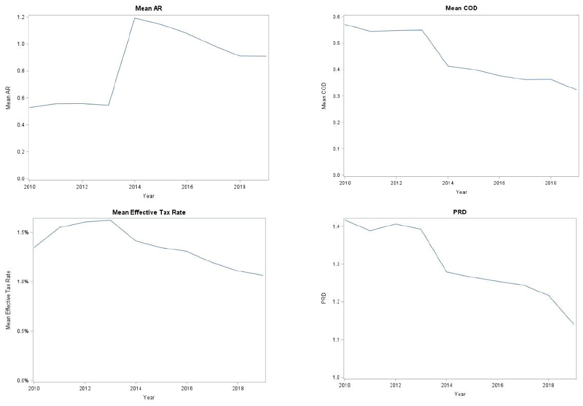
We can also look at the effective tax rate to determine how these trends in assessment
accuracy take shape in actual taxes paid. The bottom left panel of Figure 3 graphs the mean
effective tax rate over time. Post-AVI, around the same time that averages in the assessment ratio
increased and the CODs and the PRDs decreased, the average effective tax rate declined.
Contrary to these other metrics, the citywide average effective tax rate did not experience as
dramatic of a change between 2013 and 2014, but it has still steadily declined since 2013.
Figure 4 compares trends from 2012 to 2015 between Philadelphia and the control group
of 15 cities. The mean values of assessment ratio, the COD, percentage of CODs below 15
percent, and the PRD of the control group are smooth over this four-year period; Philadelphia’s
metrics trend similarly to the control group pre-AVI for all values except the PRD but diverge
from the control group post-AVI. Philadelphia’s assessed value and proportion of acceptably
accurate assessments both jumped more than twofold in 2014, whereas the control group
experienced a lower assessment ratio and only a slight improvement in acceptably accurate
assessments. Philadelphia’s mean COD and mean PRD both fell drastically in 2014, whereas
those measures each fell only very slightly in the control group.
In Figure 5, we map the COD by census tract in Philadelphia for 2013, 2014, and 2019.
The left panel shows the COD in 2013, with most tracts having high CODs. The middle panel,
for 2014, shows substantive improvement from the 2014 reassessment, but the CODs in over half
22
of the tracts were still quite high, especially in areas close to the downtown urban core. The right
panel, for 2019, shows moderate COD values across the city, indicating huge improvement
overall and a decline of the intense cross-tract variation in COD values. We can infer that even
with the AVI, one comprehensive assessment cannot solve long-accumulated issues all at once;
regular reassessment at short intervals, as well as improved quality of reassessment, is the key.
Overall, assessment accuracy improved after the AVI was adopted in 2014. As shown in
Table 1, despite the improvement in the average COD in Philadelphia following the first full
market reassessment in 2014, as well as the second full market reassessment in 2019, there was
still significant variation in CODs. This pattern implies that each comprehensive reassessment
results in a level shift — but not necessarily a trend shift — in measures of horizontal equity.
That is, each reassessment better equalizes properties of similar assessed value, but it does not
seem to systematically alter assessment practices such that there are significant improvements to
reduce the variation of assessed values from the mean.
4.2 Heterogeneity in Assessment Quality Post-AVI
To evaluate how the quality of assessment changed over time for properties in more
disadvantaged communities, we break all the sales into multiple groups based on tract-level
characteristics. Specifically, we categorize all neighborhoods in Philadelphia by median income
(in quartiles), share of White residents (in quartiles), property value (in quartiles), majority race

23
(Black, White, and other),
13
and gentrification status (gentrifying, nongentrifying, and
nongentrifiable).
14
Figure 6 shows trends in the average COD across neighborhoods, suggesting that before
the AVI was implemented, tracts that were higher income, higher value, non-Black, and
gentrifying were more likely to have a higher COD, meaning tracts with these characteristics
were more likely to have less accurate value assessments. After the AVI, however, these trends
flip. Sales in lower-income, lower home value, majority-Black and nongentrifying tracts had
higher CODs than those in other neighborhoods; that is, tracts with these characteristics were
more likely to have less accurate assessed values after the AVI.
Although this correlative trend cannot be deemed a direct result of the implementation of
the AVI, the distinction in trends across groups may suggest that changes surrounding the AVI
had a particularly negative impact on assessment quality immediately following the policy’s
implementation for already vulnerable groups (i.e., homes in majority-Black, nongentrifying,
lower-home value, and lower-income tracts). Nonetheless, the gap in the average COD across
groups appears to be converging after the adoption of the AVI, especially in more recent years.
4.3 Vertical Equity
13
Based on data from the 2009–2013 5-year American Community Survey, tracts are categorized by tract majority
race, where a tract is majority White (47 percent of observations) if the population is more than 50 percent non-
Hispanic white, majority Black (35 percent of observations) if it is more than 50 percent Black (defined as Hispanic
Black or non-Hispanic Black), and other (18 percent of observations) if it is neither majority White nor majority
Black as they are defined above.
14
Ding and Hwang (2020) define a gentrifiable tract as one in which the median household income was below that
of the city in 2000, a gentrifying tract as one which is gentrifiable and experienced both (1) an increase in either its
median gross rent or median home value above the respective city average and (2) an increase in its share of college-
educated residents from 2000 to 2013 above the average city increase, and a nongentrifying tract as one that is
gentrifiable but does not satisfy both requirements to be considered gentrifying.
24
Philadelphia’s PRD in 2010 through 2013 was between 1.39 and 1.42, clearly above the
threshold of 1.03, indicating that assessments were highly regressive in the city (Table 1 and
Figure 3, bottom right panel). In other words, lower‐priced homes were systematically assessed
at a greater percent of their market value. The long period with no reassessments and disparities
in Great Recession–induced price crashes across submarkets should help explain such high levels
of regressivity. The differential effects of the Great Recession on the various submarkets could
also have exacerbated the quality of assessment. The PRD decreased to 1.28 in 2014, indicating a
marked improvement under the AVI, but it remained regressive. The 2019 reassessment
decreased the PRD further to 1.14, showing a continued mitigation of assessment inequity.
To put the results for Philadelphia into a comparative context, the 2013 PRD of the peer
cities ranges from 0.97 in Phoenix to 1.30 in Pittsburgh (Table 2). The PRD for Pittsburgh was
only slightly lower than that for Philadelphia, likely because these two cities are in the same
state, and it does not require regular revaluations. All cities in the control group had smaller
changes in their PRD from 2013 to 2014 than did Philadelphia, with a control group average
change of -0.009 (a maximum decrease of -0.051 in Columbus City and a maximum increase of
0.034 in Baltimore, compared with a decline of 0.081 in Philadelphia). Pittsburgh had almost no
change in its PRD (from 1.30 in 2013 to 1.31 in 2014). Philadelphia’s improvement in PRD
obviously outstripped any other city in the control group, most likely because of the adoption of
the AVI. Of course, assessment inequity in Philadelphia until 2014 was still more regressive than
most of the other cities.
Collectively, the above descriptive results using the most common equity measures
suggest there was some improvement in the vertical uniformity of the property tax system

25
following reassessment. Despite that improvement, vertical inequality remains significantly
above the acceptable level.
5. Impact of the AVI on Horizontal Equity: Regression Results
This section summarizes the regression results of the short-term impact of the AVI on
horizontal equity. The AVI’s effect is captured by the coefficient of the interaction variable
(PHIL
∗
POST), representing the change in the value of the corresponding outcome measure post-
AVI of a property in Philadelphia. As defined earlier, the control group consists of residential
property sales in our 15 comparison cities. None of these cities experienced significant changes
in their property tax systems during the study period (2012–2015). Based on the observations
only in Philadelphia, we further evaluate the disparate impact of the AVI on properties in
different types of neighborhoods.
5.1. Effects of AVI on Horizontal Equity of Assessments
As shown in Table 3, we find that the AVI led to a significant improvement in horizontal
equity in residential property assessments. The adoption of the AVI in Philadelphia leads to a
decrease of 11.0 percentage points in the COD for an average property.
15
In other words, the
average COD results confirm that, compared with cities without similar comprehensive changes
in their assessment system, the adoption of more regular reassessments generally makes
assessments more uniform across properties of similar values.
15
Results from the tract-level regressions are quite consistent with the property-level results, and the magnitude is
even larger.

26
When the outcome variable is the dummy of whether the COD of a sale is below 15
percent, the results are quite consistent: The probability of having a COD below 15 percent
increases by 25.8 percentage points after the adoption of the AVI. These results confirm that the
AVI not only helps improve average assessment accuracy but it also markedly improved the
proportion of properties with acceptably accurate assessment levels. When the assessment ratio
is used as the outcome variable, the results are quite consistent; the AVI helps improve
horizontal equity by bringing the assessment ratio closer to one.
5.2. Heterogeneity in AVI’s Effect on Horizontal Equity
In Table 4, we find that the impact of the AVI on horizontal equity varies significantly
across neighborhoods in Philadelphia. Overall, the results suggest the assessment ratio decreased
after the adoption of the AVI in disadvantaged neighborhoods (majority Black,
16
low-income,
lower property value neighborhoods, as well as lower-income nongentrifying neighborhoods).
All these suggest tax assessments became fairer across neighborhoods, as assessments in these
neighborhoods experienced smaller increases (or larger declines) relative to sales prices after the
adoption the AVI than those in other neighborhoods.
The improvement in the uniformity of assessments, however, was smaller in these more
disadvantaged neighborhoods: The improvement in CODs was much smaller in majority-Black,
low-income, or lower property value neighborhoods, relative to other neighborhoods. For
example, there was a larger variation of assessment values from sales prices in majority-Black
neighborhoods, and quality of assessments in those neighborhoods even became slightly worse
16
Note that here, tracts are categorized by the “majority Black,” or simply “Black,” binary variable, in which a tract
is Black (35 percent of observations) if it is more than 50 percent Black (defined as Hispanic Black or non-Hispanic
Black), and it is non-Black (65 percent of observations) if it is not majority Black as defined above.

27
post-AVI: The percent of sales with a COD below 15 percent decreased by 24.9 percentage
points in majority-Black neighborhoods relative to non-Black neighborhoods.
When we use yearly dummies instead of one POST dummy, the results confirm that the
uniformity in assessment, as measured by the COD, becomes relatively worse in majority-Black
neighborhoods, especially in the initial years after the AVI was adopted. The assessment ratio
and the COD in majority-Black neighborhoods experience a relatively larger increase
immediately after the adoption of the AVI (2014 and 2015) than in later years. This could be
partly explained by the generally larger variation of assessment among low-value properties.
This may also be attributed to the methodology, data reporting, or other aspects of the property
valuation practices that may affect the quality of property assessments. While property tax
horizontal uniformity has improved over time, the change in the COD in majority-Black
neighborhoods from the pre-AVI level was still significantly larger than that in majority-White
neighborhoods as of 2019 (by 22 percent). Similar patterns can be found for properties using
other measures of neighborhood disadvantages, such as lower-income neighborhoods, high-
minority neighborhoods, neighborhoods with lower property values, or nongentrifying
neighborhoods. It is concerning if such an assessment system makes low-income and
predominantly minority neighborhoods more vulnerable. More research is warranted regarding
additional interventions to mitigate potential disparate impacts of more frequent reassessment.
5.3. Effects of the AVI on Horizontal Equity of Property Owners’ Tax Burdens
In terms of the actual tax burden for property owners, compared with other cities, the
effective tax rate did not experience significant changes after the adoption of the AVI, as shown

28
in Table 3. This is consistent with the claim by the city government that the AVI is largely a
revenue-neutral policy.
However, the impact of the AVI on tax burdens varies significantly across neighborhoods
(Table 4). In fact, properties in majority-Black neighborhoods, high-minority neighborhoods,
low-income neighborhoods, and nongentrifying neighborhoods saw a larger decrease in their
effective tax rate relative to those in other more advantaged neighborhoods. Taken together with
the PRD results presented above, these results suggest the AVI generally makes property taxes
more equitable in Philadelphia. This is especially evident in the model using yearly dummies,
which suggests the effective tax rate declines over time post-AVI in majority-Black
neighborhoods relative to the non-Black ones (from -0.334 percentage point in 2014 to -0.753
percentage point in 2019). The results suggest that while property owners in less advantaged
neighborhoods experienced patterns of worsening uniformity of assessment, the improvement in
tax burden for property owners in the same neighborhoods continued even after the adoption of
the AVI.
In addition to improving the quality of assessments, the regressivity of the property tax
can also be mitigated by well-targeted tax relief programs. For example, the AVI was adopted
together with two major programs: one to mitigate tax increases for owner-occupied
homeowners (the Homestead Exemption program)
17
and one for long-term homeowners who
were likely to face sharp increases in property tax bills after the reassessments (the Longtime
Owner Occupants Program or LOOP). The Homestead Exemption program should make
property taxation more progressive, since the amount of the exemption is fixed regardless of the
value of the property; thus, homeowners of lower-value properties enjoy larger benefits from the
17
The Homestead Exemption program, the biggest single mitigation program, is available for all owner-occupied
primary residences in Philadelphia, regardless of the homeowner’s income or length of tenure in their residences.
29
program. In contrast, certain tax programs may increase the regressivity of property taxes. For
example, Philadelphia has an abatement program that was enacted in 1997, under which new
construction or major rehabilitation projects are entitled to a 10-year tax abatement on the value
of the newly constructed or rehabilitated improvements.
6. Conclusion
Despite decades of property tax revolts, local governments continue to rely heavily on
property taxes. Property assessment, however, is a complex and constantly evolving field and
there has been no consensus on whether property values should be regularly reassessed to assure
the equity of the real property tax. In practice, many U.S. states do not mandate regular
revaluation cycles — at least not short, regular cycles. During long intervals between
assessments, property values in urban centers diverge widely: Those in wealthy districts and
prime locations appreciate quickly, whereas those in poor districts and less desirable locations
rise very little, if at all. Recessions could also exacerbate the quality of overall property
assessment when assessments do not keep up with sharper declines in property values in harder-
hit areas. Thus, taxes that are levied at the same rate but are based on outdated valuations may
hurt low-income homeowners.
The empirical results show generally positive evidence of regular revaluations, although
impacts appear to vary across neighborhood types. The quality of assessments in Philadelphia, as
measured by the COD, improves significantly after the revaluation in 2014. The tax burden for
properties in less advantaged neighborhoods was also reduced after the AVI was introduced,
although an alternative vertical equity measure presents mixed results. These results highlight the
importance of regular reassessment in cities experiencing significant increases in property values

30
(i.e., gentrification) and shed light on the disparate impacts that reassessment might have across
income, property value, race, and gentrification.
While our findings suggest that more regular reassessments do improve vertical and
horizontal equity, such a program does not address all the challenges of property assessment or
property tax administration. The quality of assessment of Philadelphia properties, although
significantly improved post-AVI, is still far above the acceptable threshold. This could be
explained by variations in assessment methodologies or issues related to quality control, data
collection, and data cleaning for property transactions.
Discussions of city- and state-level revaluation policy changes have been in the works for
some time. At the national level, regular revaluation of properties has been required by the real
property tax law in most states. At the state level, a 2010 study of county assessment practices in
Pennsylvania recommended that the Pennsylvania General Assembly consolidate property
assessment law into a uniform statewide system and require more frequent reassessment at an
interval of four years (Weber et al., 2010). Such changes could not only improve assessment
quality and equity across all counties in Pennsylvania but also lower the administrative costs of
reassessment, simplify processes to mitigate human error, and comply with the state
constitution’s uniformity clause.
At the city level, the Philadelphia City Council recommended in 2019 that the OPA
overhaul its leadership, partner with private firms to increase assessment accuracy and appraisal
services, and reform its quality control methods (Clarke, 2019). The Office of the Controller also
advised that OPA targets its efforts on the geographic areas that are most disproportionately tax
burdened — North, Southwest, and West Philadelphia (Rhynhart, 2019). It also recommended
readdressing land valuations, improving the transparency of assessment methods, and examining
31
the true impact of the current tax exemptions and abatements aimed to protect vulnerable
homeowners. The city also hired consultants in 2019 to evaluate the city’s property assessment
system (J.F. Ryan Associates, Inc., 2018). Based on recommendations from the evaluation, the
city initially planned to implement a new assessment system in 2020, which has been delayed
because of the COVID-19 crisis. Approaches such as these city- and state-level policy proposals
may help fill the equity gaps that the AVI hasn’t managed to mitigate in Philadelphia’s property
tax system.
This paper provides updated evidence on the equity effects (horizontal and vertical) of
property revaluation on the distribution of the tax burden among owners along the income
spectrum after a long lapse in reassessments. The paper makes the case that the real property tax
can be well maintained as an effective tax instrument, although other practices or tax relief
programs might be necessary to ensure an equitable impact. Despite conventional taxation theory
holding equity and efficiency as tradeoffs, the evidence presented supports the idea that equity
and efficiency can improve in unison, such that each reinforces the other through more frequent,
regular property tax reassessments. As a case study, this empirical research contributes to
debates on the design of property taxation systems. The results can help researchers and
policymakers understand the complicated relationship between property sales, assessments, and
property taxes.

32
References
Advisory Commission on Intergovernmental Relations (ACIR) 1987. Changing Attitudes on
Governments and Taxes. Washington, D.C.: Government Printing Office.
Alm, J., Hawley, Z., Lee, J.M., Miller, J.J., 2016. Property Tax Delinquency and Its Spillover
Effects on Nearby Properties,” Regional Science and Urban Economics, 58: pp. 71–7.
Alm, J., Hodge, T.R., Sands, G., Skidmore, M., 2014. “Detroit Property Tax Delinquency: Social
Contract in Crisis,” Public Finance and Management, 14(3): pp. 280–305.
Almy, R.R., International Association of Assessing Officers, 1978. Improving Real Property
Assessment: A Reference Manual. Chicago: The Association.
Anderson N.B., Dokko, J.K., 2016. “Liquidity Problems and Early Payment Default Among
Subprime Mortgages,” Review of Economics and Statistics, 98(5): pp. 897–912.
Bell, E.J., 1984. “Administrative Inequity and Property Assessment: The Case for the Traditional
Approach,” Property Tax Journal, 3: pp. 123–31.
Berry, C., Schmidt, M., Langowski, E., Wang, X., Rockower, J., 2021. Property Tax Fairness
from the Center of Municipal Finance, Harris School of Public Policy, University of
Chicago. Available at propertytaxproject.uchicago.edu/.
Bowman, J.H., Mikesell, J.L., 1990. “Improving Administration of the Property Tax: A Review
of Prescriptions and Their Impacts,” Public Budgeting and Financial Management, 2(2): pp.
151–76.
Cabral, M., Hoxby, C., 2012. “The Hated Property Tax Salience, Tax Rates, and Tax Revolts,”
NBER Working Paper No. 18514.
Carter, J.M., 2016. “Methods for Determining Vertical Inequity in Mass Appraisal,” Fair &
Equitable, 14(6): pp. 3–8.
Cheng, P.L., 1974. “Property Taxation, Assessment Performance, and Its Measurement,” Public
Finance, 29: pp. 268–84.
Clarke, D.L., 2019. “Council Releases Recommendations for Property Assessment,”
Philadelphia City Council. Available at phlcouncil.com/council-releases-recommendations-
for-property-assessment-reforms-following-independent-audit/.
Deboer, L., Conrad, J., 1988. “Do High Interest Rates Encourage Property Tax Delinquency?”
National Tax Journal, 41(4): pp. 555–60.
Ding, L., Hwang, J., 2020. “Effects of Gentrification on Homeowners: Evidence from a Natural
Experiment,” Discussion paper, Community Development and Regional Outreach, Federal
Reserve Bank of Philadelphia.
Dowdall, E., 2015. The Actual Value Initiative: Philadelphia’s Progress on Its Property Tax
Overhaul, Philadelphia: The Pew Charitable Trusts. Available at
www.pewtrusts.org/~/media/assets/2015/09/philadelphia-avi-update-brief.pdf.

33
Dowdall, E., Warner, S., 2012. The Actual Value Initiative: Overhauling Property Taxes in
Philadelphia, Philadelphia: The Pew Charitable Trusts. Available at
www.pewtrusts.org/~/media/legacy/uploadedfiles/
wwwpewtrustsorg/reports/philadelphia_research_initiative/philadelphiapropertytaxespdf.pdf.
Eom, T.H., 2008. “A Comprehensive Model of Determinants of Property Tax Assessment
Quality: Evidence in New York State,” Public Budgeting and Finance, 28(1): pp. 58–81.
Ferreira, F., Gyourko, J., 2009. “Do Political Parties Matter? Evidence from U.S.
Cities,” Quarterly Journal of Economics, 124(1): pp. 399–422.
Fisher, G.W., 1996. The Worst Tax? A History of the Property Tax in America. Lawrence, KS:
University Press of Kansas.
Geraci, V.J., 1977. “Measuring the Benefits from Property Tax Assessment Reform,” National
Tax Journal, 30: pp. 195–205.
Gillen, K.C., 2008. “Updated Results on Property Assessment Accuracy, Uniformity and Equity
in Philadelphia,” Econsult Corporation. Available at
media.philly.com/documents/taxproj07gillen08.pdf.
Gloudemans, R.J., 1999. Mass Appraisal of Real Property. Chicago: International Association of
Assessing Officers.
Higginbottom, J., 2010. State Provisions for Property Reassessment. Washington, D.C.: Tax
Foundation.
International Association of Assessing Officers, 2013. Standard on Ratio Studies. Kansas City,
MO: IAAO.
J.F. Ryan Associates, Inc., 2018. Council of the City of Philadelphia – 2019 Property Assessment
Audit. Newburyport, MA: J.F. Ryan Associates, Inc.
Jensen, J.P., 1931. Property Taxation in the United States. Chicago: University of Chicago Press.
Kochin, L.A., Parks, R.W., 1982. "Vertical Equity in Real Estate Assessment: A Fair
Appraisal?” Economic Inquiry, 20: pp. 511–32.
Langley, A.H., 2018. “Improving the Property Tax by Expanding Options for Monthly
Payments,” Lincoln Institute of Land Policy Working Paper No. 18AL1.
McMillen, D., 2013. “The Effect of Appeals on Assessment Ratio Distributions: Some
Nonparametric Approaches,” Real Estate Economics, 41(1): pp. 165–91.
McMillen, D., Singh, R., 2020. “Assessment Regressivity and Property Taxation,” Journal of
Real Estate Finance and Economics, 60: 155–69.
Mikesell, J.L., 1980. “Property Tax Reassessment Cycles: Significance for Uniformity and
Effective Rates,” Public Finance Quarterly, 8(1): pp. 23–37.
Miller, J.J., 2012. The Cost of Delinquent Property Tax Collection. University of Illinois at
Chicago: Dissertation.

34
Montarti, E., Weaver, E., 2007. Pennsylvania’s Property Assessment System Needs Change,
Pittsburgh: Allegheny Institute for Public Policy, Report No. 07-07.
O’Flaherty, B., 1990. “The Option Value of Tax Delinquency: Theory,” Journal of Urban
Economics, 28(03): pp. 287–317.
Paglin, M., Fogarty, M., 1972. “Equity and the Property Tax: A New Conceptual Focus,”
National Tax Journal, 25: pp. 557–66.
Property Assessment Reform Task Force, 2018. “Pennsylvania Property Assessment: A Self-
Evaluation Guide for County Officials,” Pennsylvania Local Government Commission.
Rhynhart, R., 2019. “The Accuracy and Fairness of Philadelphia’s Property Assessments,”
Office of the Controller. Available at controller.phila.gov/philadelphia-audits/property-
assessment-review/.
Simonsen, B., Robbins, M.D., Helgerson, L., 2001. “The Influence of Jurisdiction Size and Sale
Type on Municipal Bond Interest Rates: An Empirical Analysis,” Public Administration
Review, 61(6): pp. 709–17.
Sternlieb, G., 1972. The Urban Housing Dilemma. New York: Housing and Development
Administration.
Sternlieb, G., Lake, R.W., 1976. “The Dynamics of Real Estate Tax Delinquency,” National Tax
Journal, 29(3): pp. 261–71.
Sunderman, M., Birch, J., Cannaday, R., Hamilton, T., 1990. “Testing for Vertical Inequity in
Property Tax Systems,” Journal of Real Estate Research, 5(3): pp. 319–34.
Swierenga, R.P., 1976. Acres for Cents: Delinquent Tax Auctions in Domestic Iowa. Westport,
CT: Greenwood Press.
Waldhart, P., Reschovsky, A., 2012. “Property Tax Delinquency and the Number of Payment
Installments,” Public Finance and Management, 12(4): pp. 316–30.
Weber, J.A., Scott, L., Andersen, C., Dakouri, M., et al., 2010. Pennsylvania County Property
Reassessment: Impact on Local Government Finances and the Local Economy, Harrisburg,
PA: The Center for Rural Pennsylvania. Available at
www.rural.palegislature.us/county_reassessment_2010.pdf.
Whitaker, S., Fitzpatrick, T.J., 2013. “Deconstructing Distressed-Property Spillovers: The
Effects of Vacant, Tax-Delinquent, and Foreclosed Properties in Housing
Submarkets,” Journal of Housing Economics, 22(2): pp. 79–91.

35
Figure 1: Mean Sales Prices and Mean Assessments of Single-Family Residential Properties in Philadelphia, 2010–2019
Source: Authors’ calculations using data on property assessments, tax payment history, and sales transactions from the City of Philadelphia’s Department of Revenue, Department
of Records, and Office of Property Assessment.

36
Figure 2. Philadelphia Coefficient of Dispersion (COD) Distribution in 2013, 2014, and 2019
Source: Authors’ calculations using data on property assessments, tax payment history, and sales transactions from the City of Philadelphia’s Department of Revenue, Department
of Records, and Office of Property Assessment.
37
Figure 3: Mean Assessment Ratio, Coefficient of Dispersion, Effective Tax Rate, and Price-Related Differential, Philadelphia
Source: Authors’ calculations using data on property assessments, tax payment history, and sales transactions from the City of Philadelphia’s Department of Revenue, Department
of Records, and Office of Property Assessment.

38
Figure 4: Measures of Horizontal Equity and Vertical Equity, Philadelphia vs. Control Group of Cities, 2012–2015
Source: Authors’ calculations using data on property assessments, tax payment history, and sales transactions from the City of Philadelphia’s Department of Revenue, Department
of Records, and Office of Property Assessment, and national control city data from CoreLogic Solutions.

39
Figure 5. Average Coefficient of Dispersion (COD) in Philadelphia by Neighborhood in 2013, 2014, and 2019
Source: Authors’ calculations using data on property assessments, tax payment history, and sales transactions from the City of Philadelphia’s Department of Revenue, Department
of Records, and Office of Property Assessment, and U.S. Census TIGER/Line Shapefiles.

40
Figure 6. Coefficient of Dispersion (COD) Trends by Neighborhood Characteristics
Source: Authors’ calculations using data on property assessments, tax payment history, and sales transactions from the City of Philadelphia’s Department of Revenue, Department
of Records, and Office of Property Assessment, and 2009-2013 American Community Survey data.

41
Table 1: Descriptive Statistics for Sales in Philadelphia
(1) (2) (3) (4) (5) (6) (7) (8) (9)
Year
# of
Sales
Mean
Sale
Price
Mean
Assessm
ent
Mean
Tax
Amount
Mean
AR
Mean
COD
Percent
COD
< 15%
PRD
Mean
Effective
Tax
Rate
2010 12,596 $137,884 $51,640 $1,179 0.53 0.57 0.07 1.42 1.34%
2011 11,363 $133,575 $53,694 $1,329 0.56 0.54 0.09 1.39 1.55%
2012 12,029 $140,307 $55,774 $1,413 0.56 0.55 0.07 1.41 1.61%
2013 13,381 $145,997 $57,369 $1,492 0.55 0.55 0.08 1.39 1.62%
2014 13,517 $165,434 $154,299 $1,655 1.19 0.41 0.33 1.28 1.41%
2015 15,756 $164,414 $149,106 $1,622 1.15 0.40 0.33 1.27 1.35%
2016 18,455 $172,862 $148,670 $1,679 1.08 0.38 0.34 1.25 1.31%
2017 20,040 $187,057 $148,588 $1,694 0.99 0.36 0.31 1.25 1.19%
2018 20,102 $196,348 $147,089 $1,700 0.91 0.36 0.25 1.22 1.11%
2019 18,932 $202,013 $161,284 $1,855 0.91 0.32 0.29 1.14 1.06%
Source: Authors’ calculations using data on property assessments, tax payment history, and sales transactions from the City of
Philadelphia’s Department of Revenue, Department of Records, and Office of Property Assessment.

Table 2: Descriptive Statistics in Philadelphia and Peer Cities
Total Sales Mean Sales Mean Assessment Mean AR Mean COD
Pct COD
Below 15%
PRD
Mean
Effective Tax
Rate
2013
2014
2013
2014
2013
2014
2013
2014
2013
2014
2013
2014
2013
2014
2013
2014
Philadelphia 13,381 13,517 $145,997 $165,434 $57,369 $154,299 0.55 1.19 0.55 0.41 0.08 0.33 1.39 1.28 1.62% 1.41%
Baltimore 8,144 5,629 $153,624 $138,851 $149,504 $131,912 1.26 1.27 0.52 0.54 0.25 0.21 1.29 1.34 2.95% 2.93%
Charlotte 15,196 13,828 $209,967 $226,544 $197,080 $195,958 1.05 0.96 0.26 0.24 0.50 0.49 1.12 1.11 1.37% 1.27%
Columbus 17,731 13,084 $135,482 $148,748 $134,761 $141,799 1.24 1.13 0.40 0.30 0.41 0.48 1.24 1.18 2.78% 3.25%
Dallas 12,505 9,420 $263,046 $263,703 $230,791 $226,348 0.94 0.89 0.24 0.23 0.42 0.41 1.07 1.04 2.54% 2.43%
Denver 12,336 10,038 $332,432 $368,169 $274,531 $276,218 0.84 0.76 0.21 0.27 0.40 0.22 1.02 1.01 0.58% 0.52%
El Paso 4,273 2,833 $150,385 $148,010 $149,543 $145,510 1.06 1.04 0.21 0.20 0.54 0.53 1.07 1.06 3.40% 2.86%
Fort Worth 11,301 5,825 $165,997 $159,691 $150,785 $137,366 0.96 0.90 0.20 0.21 0.53 0.49 1.06 1.05 2.77% 2.60%
Houston 25,053 24,668 $238,696 $254,692 $207,874 $226,551 0.93 0.94 0.22 0.22 0.45 0.46 1.07 1.05 2.56% 2.52%
Oklahoma City 11,893 12,047 $147,955 $157,418 $141,558 $156,444 1.07 1.09 0.25 0.19 0.59 0.75 1.11 1.09 1.29% 1.25%
Phoenix 29,385 17,531 $206,105 $215,219 $113,231 $124,470 0.53 0.57 0.48 0.44 0.03 0.03 0.97 0.98 0.72% 0.70%
Pittsburgh 3,508 3,154 $142,009 $160,418 $116,743 $125,583 1.07 1.03 0.40 0.39 0.28 0.26 1.30 1.31 2.55% 2.09%
Portland 11,242 10,210 $331,552 $348,896 $296,005 $324,654 0.94 0.97 0.18 0.17 0.51 0.58 1.05 1.04 1.34% 1.30%
San Antonio 14,543 9,333 $174,423 $194,937 $158,143 $174,734 0.95 0.93 0.21 0.20 0.50 0.52 1.04 1.04 2.50% 2.43%
Seattle 10,358 8,129 $473,597 $512,510 $371,149 $389,338 0.83 0.79 0.25 0.25 0.26 0.22 1.06 1.04 0.97% 0.87%
Washington, D.C. 6,862 5,331 $546,066 $546,573 $449,642 $450,541 0.88 0.87 0.24 0.23 0.38 0.39 1.07 1.05 0.76% 0.68%
Source: Authors’ calculations using data on property assessments, tax payment history, and sales transactions from the City of Philadelphia’s Department of Revenue, Department
of Records, and Office of Property Assessment, and national control city data from CoreLogic Solutions.
43
Table 3. Summary of Coefficients of the Interaction Terms (Peer City Comparison)
Source: Authors’ calculations using data on property assessments, tax payment history, and sales transactions from the City of Philadelphia’s Department of Revenue, Department
of Records, and Office of Property Assessment, and national control city data from CoreLogic Solutions.
Assessment Ratio
COD COD_pct15 Effectiv e T ax Rate
Coef. Std. Err. t P>t Coef. Std. Err. t P>t Coef. Std. Err. t P>t Coef. Std. Err. t P>t
Treat -0.338 0.013 26.910 0.000 0.045 0.006 8.230 0.000 -0.343 0.007 48.420 0.000 -0.028 0.024 1.160 0.265
Post_14 -0.062 0.024 2.540 0.023 -0.032 0.011 3.000 0.009 0.000 0.014 0.010 0.992 -0.165 0.048 3.460 0.004
Treat*Post_14 0.706 0.024 28.880 0.000 -0.110 0.011 10.190 0.000 0.258 0.014 18.680 0.000 -0.014 0.048 0.290 0.775

44
Table 4. Summary of the Coefficients of the Interaction Terms (Philadelphia Properties Only)
Source: Authors’ calculations using data on property assessments, tax payment history, and sales transactions from the City of Philadelphia’s Department of Revenue, Department
of Records, and Office of Property Assessment.
Assessment Ratio COD COD_pct15 Effectiv e Tax Rate
Coef. Std. Err. t P>t C oef. Std. Err. t P>t C oef. Std. Err. t P>t Coef. Std. Err. t P>t
Black NBH D (v s N on-black) -0.063 0.018 -3.500 0.001 0.282 0.019 14.720 0.000 -0.249 0.015 -16.090 0.000 -0.475 0.043 -11.030 0.000
Tract Share of White
1st quartile (v s upper quartile) -0.031 0.023 -1.380 0.170 0.443 0.015 29.730 0.000 -0.341 0.020 -17.050 0.000 -0.694 0.050 -14.000 0.000
2nd quartile (v s upper quartile) -0.047 0.021 -2.240 0.026 0.322 0.021 15.470 0.000 -0.253 0.023 -10.930 0.000 -0.487 0.053 -9.140 0.000
3rd quartile (v s upper quartile) -0.006 0.018 -0.320 0.753 0.122 0.021 5.830 0.000 -0.079 0.025 -3.110 0.002 -0.137 0.041 -3.330 0.001
Tract income
1st quartile (v s upper quartile) -0.065 0.024 -2.750 0.006 0.415 0.024 17.290 0.000 -0.345 0.019 -18.080 0.000 -0.745 0.061 -12.190 0.000
2nd quartile (v s upper quartile) -0.008 0.020 -0.410 0.684 0.300 0.023 13.020 0.000 -0.252 0.023 -10.980 0.000 -0.449 0.048 -9.440 0.000
3rd quartile (v s upper quartile) 0.021 0.017 1.260 0.207 0.128 0.019 6.590 0.000 -0.098 0.023 -4.240 0.000 -0.191 0.039 -4.940 0.000
Property v alue
1st quartile (v s upper quartile) -0.149 0.018 -8.150 0.000 0.461 0.014 32.390 0.000 -0.378 0.015 -25.610 0.000 -0.988 0.040 -24.600 0.000
2nd quartile (v s upper quartile) 0.044 0.014 3.240 0.001 0.292 0.016 18.300 0.000 -0.229 0.017 -13.400 0.000 -0.340 0.026 -13.250 0.000
3rd quartile (v s upper quartile) 0.043 0.009 4.700 0.000 0.091 0.010 8.790 0.000 -0.062 0.016 -3.980 0.000 -0.142 0.022 -6.420 0.000
Gentrification
Nongentrifying (v s nongentrifiable) -0.089 0.017 -5.090 0.000 0.328 0.020 16.640 0.000 -0.299 0.015 -20.220 0.000 -0.621 0.046 -13.610 0.000
Gentrify ing (v s nongentrifiable) -0.142 0.024 -5.850 0.000 -0.021 0.025 -0.830 0.408 -0.152 0.022 -6.840 0.000 0.028 0.056 0.500 0.619
Nongentrifying (v s gentrify ing) 0.058 0.028 2.040 0.042 0.351 0.027 13.130 0.000 -0.151 0.021 -7.180 0.000 -0.642 0.068 -9.440 0.000

45
Table 5. Summary of the Coefficients of the Interaction Terms (Year 2013 as Reference, Philadelphia Properties Only)
Source: Authors’ calculations using data on property assessments, tax payment history, and sales transactions from the City of Philadelphia’s Department of Revenue, Department
of Records, and Office of Property Assessment.
AR COD COD_pct15 Effectiv e Tax Rate
Coef. Std. Err. t P>t Coef. Std. Err. t P>t Coef. Std. Err. t P>t Coef. Std. Err. t P>t
Black NBHD*2010 -0.009 0.018 -0.490 0.623 -0.019 0.011 -1.750 0.081 0.002 0.011 0.180 0.854 -0.142 0.059 -2.390 0.017
Black NBHD*2011 -0.004 0.015 -0.280 0.778 -0.005 0.009 -0.590 0.554 -0.007 0.009 -0.730 0.465 -0.068 0.049 -1.380 0.169
Black NBHD*2012 -0.004 0.012 -0.310 0.755 0.001 0.008 0.070 0.942 -0.017 0.009 -1.900 0.058 -0.030 0.041 -0.740 0.460
Black NBHD*2014 0.059 0.025 2.340 0.020 0.334 0.029 11.630 0.000 -0.273 0.021 -12.840 0.000 -0.334 0.067 -5.010 0.000
Black NBHD*2015 0.022 0.023 0.960 0.336 0.314 0.028 11.190 0.000 -0.276 0.021 -13.240 0.000 -0.401 0.059 -6.850 0.000
Black NBHD*2016 -0.031 0.022 -1.420 0.158 0.297 0.025 11.910 0.000 -0.284 0.022 -13.190 0.000 -0.478 0.058 -8.240 0.000
Black NBHD*2017 -0.071 0.022 -3.210 0.001 0.277 0.021 13.390 0.000 -0.263 0.019 -13.670 0.000 -0.547 0.059 -9.290 0.000
Black NBHD*2018 -0.106 0.021 -4.990 0.000 0.244 0.016 14.880 0.000 -0.204 0.015 -13.220 0.000 -0.588 0.063 -9.330 0.000
Black NBHD*2019 -0.207 0.022 -9.540 0.000 0.220 0.018 12.070 0.000 -0.237 0.017 -13.670 0.000 -0.753 0.077 -9.780 0.000
